Energy Consumption and Economic Performance in a Spatial Context: Spillover Effects Across Borders

Abstract

Extensive research has delved into the interplay between energy consumption and economic development. Building upon this rich literature, this paper revisits this nexus from a spatial perspective that emphasizes cross-country interdependencies and spatial dynamics. We utilize a dataset of 103 countries spanning 1990–2015, treating this period as a historically coherent benchmark preceding the major shift in the international climate-policy environment associated with the Paris Agreement and the United Nations 2030 Agenda. Our empirical findings reveal a robust and positive relationship between renewable energy consumption, non-renewable energy consumption, and GDP per capita within a country, consistent with findings in the existing literature. Furthermore, employing a unified spatial model, our study uncovers cross-country spillover effects through geographical proximity, energy consumption similarity, and economic linkages. Notably, the results reveal negative spatial spillover associations between energy consumption in neighboring countries and the home country’s GDP per capita. Potential explanations for these negative spillover effects include increased emissions from neighboring countries, which may impose health and economic burdens on the home country, and the possibility that Renewable Energy Technology Innovation (RETI) promotes local green industrial advancement while limiting similar progress in neighboring countries.

1. Introduction

Since 2015, the Sustainable Development Goals (SDGs) have established the 2030 Agenda, a global framework aimed at transforming our world by addressing the pressing challenges we face today (Pradhan et al., 2017). In order to attain the Sustainable Development Goals (SDGs), particularly focusing on SDG 7 (addressing climate change) and SDG 13 (ensuring energy sustainability), it is imperative for all nations worldwide to collectively shoulder the responsibility. Thus, the increasing awareness of climate change, environmental degradation (including air and water pollution), volatile energy prices, and the finite nature of non-renewable resources underscores the pressing need to transition to cleaner and more sustainable energy sources (Owusu & Asumadu-Sarkodie, 2016; IEA, 2022). Comprehending the intricate relationships and consequences of these factors is imperative for tackling the complex challenges posed by climate change, all while fostering sustainable economic progress. As a result, examining how renewable and non-renewable energy use relates to economic development is highly significant for research in both energy and economics fields (Elavarasan et al., 2022).

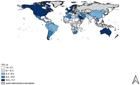
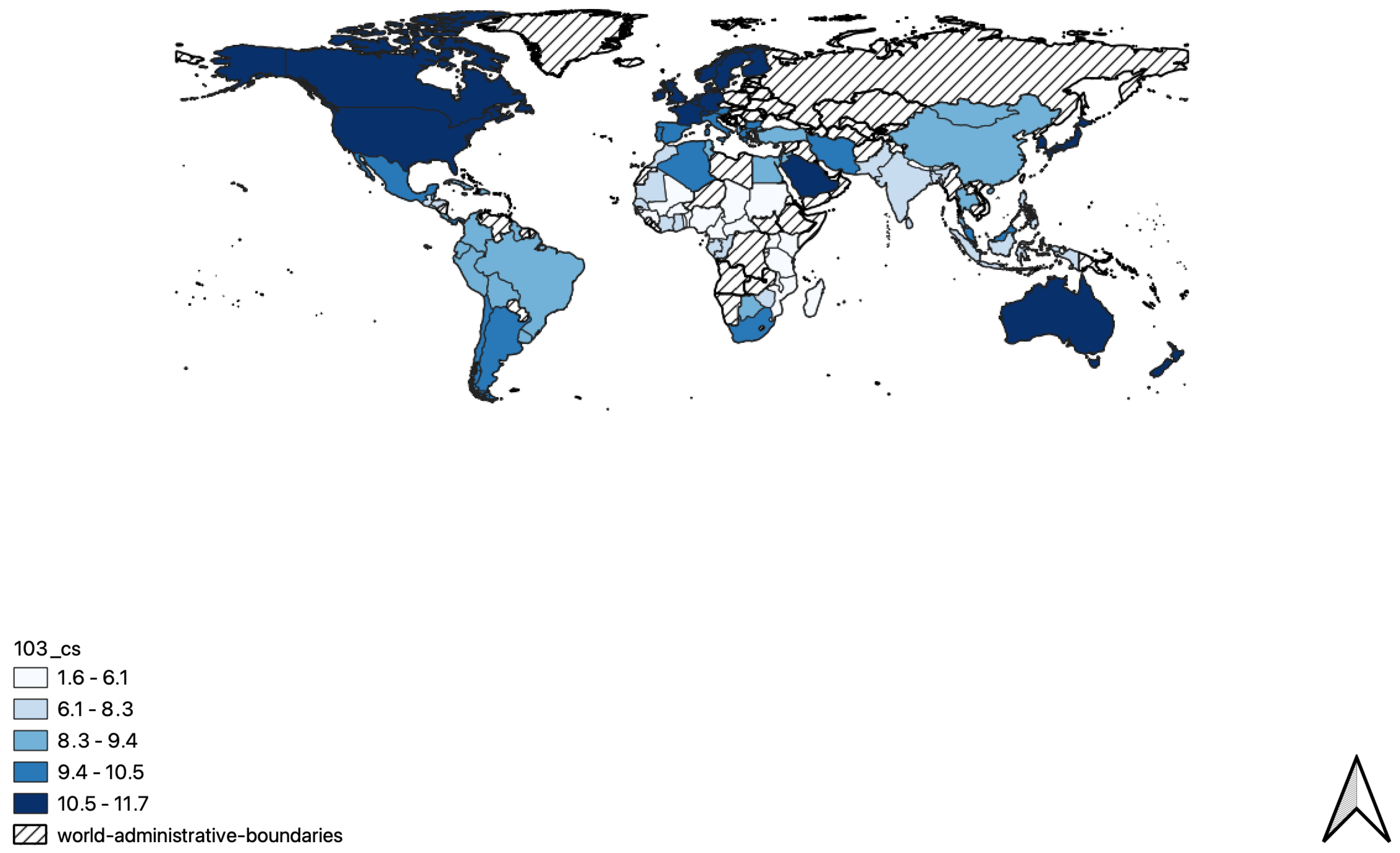
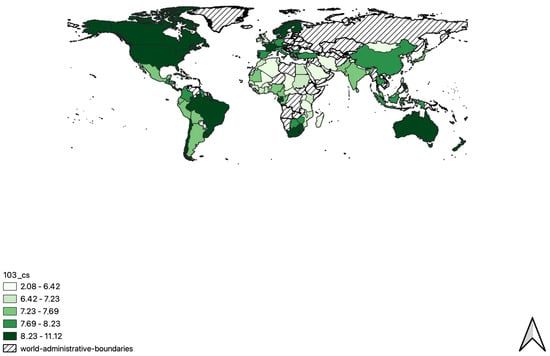
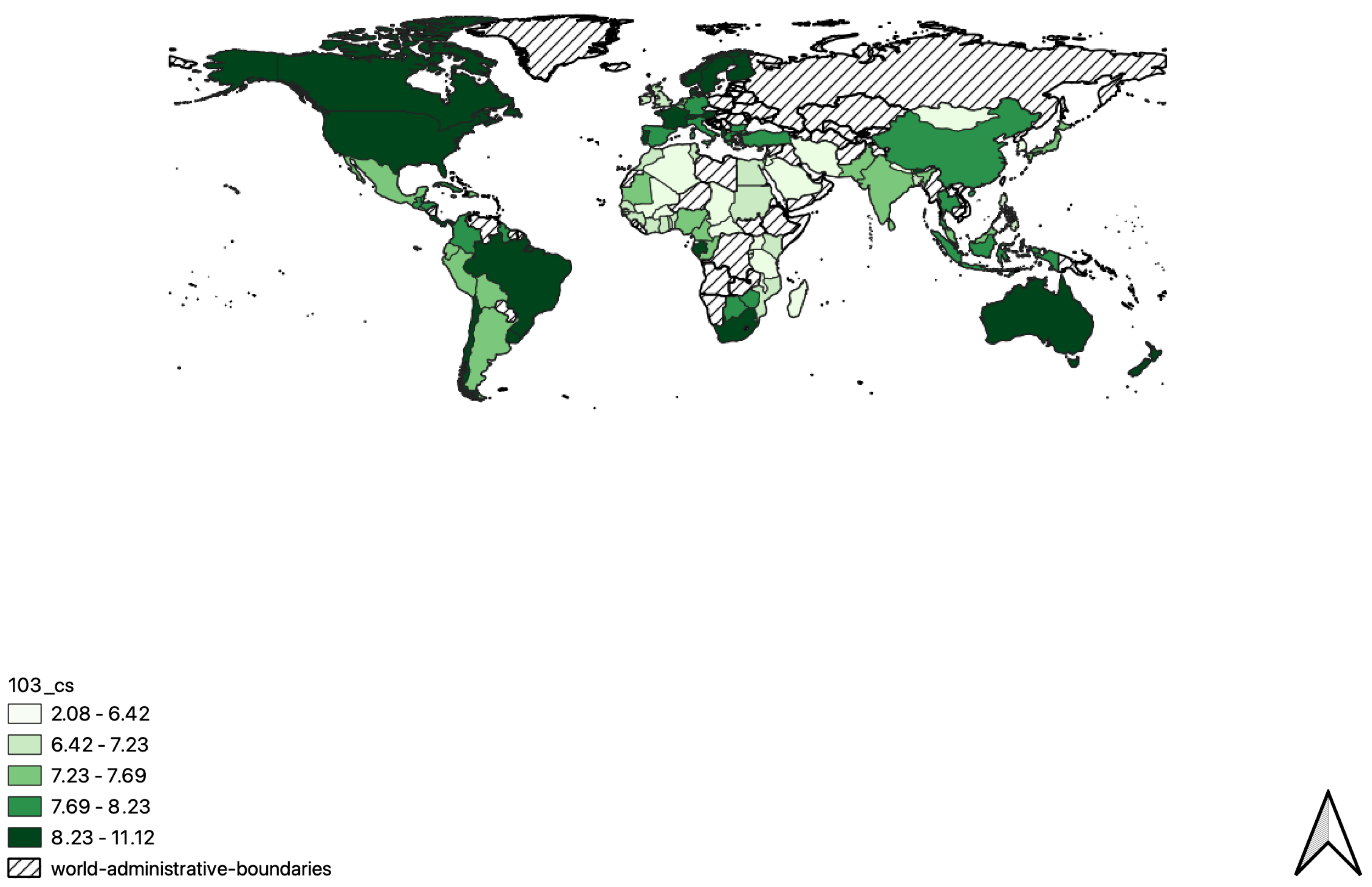
Evidently, in terms of energy consumption, developed countries exhibit a considerably higher per capita consumption of non-renewable energy on a global scale. Figure 1 shows the natural log value of the average non-renewable per capita energy consumption from 1990 to 2015 across 103 selected countries. Figure 2 illustrates the natural log of the average per capita renewable energy consumption across the same countries and time period. Likewise, developed countries also show significantly higher consumption levels of renewable energy. It is noteworthy that the consumption patterns for both renewable and non-renewable energy are surprisingly consistent. Hence, this observation also underscores the fact that the predominant consumers of non-renewable energy like the United States, Canada, China, and Australia also tend to be the leading consumers of renewable energy worldwide, which emphasizes the pivotal role of energy consumption within the economy (Cleveland et al., 2000). Furthermore, Figure 1 and Figure 2 clearly indicate that geographically adjacent countries tend to exhibit more similar energy consumption patterns. Similarly, it is also noteworthy that countries that are economically or energy-consumption-similarity proximate also tend to share more comparable energy consumption patterns. For instance, in the European area, most national policy supports in the renewable energy policies become increasingly similar (Kitzing et al., 2012). Thus, it is intuitive that if countries have similar energy policies, it is highly likely that the energy consumption per capita levels will be similar. Likewise, if countries have the same level of economic development, the energy consumption per capita levels are highly likely to be more comparable. Hence, the increasing globalization in the past decades makes us think about the potential spillovers between these geographical, energy consumption similarity, and economic neighbors become crucial in this context. Crucially, against the backdrop of global climate change, investigating the intricate relationship between the energy consumption patterns of “neighboring” countries and the economies of home countries assumes heightened significance within this context.

Figure 1. Non-renewable energy consumption per capita.

Figure 2. Renewable energy consumption per capita.

An important feature of the empirical design is the choice of the 1990–2015 study period. Rather than treating this period as representative of current global energy conditions, we use it as a historically coherent benchmark covering the period prior to the major shift in the international climate-policy environment associated with the Paris Agreement and the United Nations 2030 Agenda in 2015. This distinction is particularly relevant in a spatial setting, since subsequent changes in national energy policies, renewable energy deployment, and international economic linkages may alter not only domestic energy–economic relationships but also the structure of cross-country spillovers. Accordingly, the objective of this study is to characterize the spatial energy–economic nexus during this pre-Paris/pre-SDG period and to provide a historical benchmark against which subsequent developments may be evaluated.

Against this background, and building on the energy consumption–economic development literature exemplified by Apergis and Payne (2010a), this study revisits the relationship between renewable energy consumption and economic development while explicitly incorporating non-renewable energy consumption as a separate explanatory variable. This paper contributes to the existing literature through several channels. First, this paper focuses on a global scale and selects 103 countries in the world to study how and to what extent renewable energy consumption and non-renewable energy consumption are in connection with economic development. Second, since this paper aims to investigate the potential spillovers and how neighboring countries’ consumption affects home countries’ economies, this paper introduces a spatial model into the analysis and examines how the estimated spillover effects vary across years. Third, this paper not only includes a typical geographical spatial weight matrix but includes multiple spatial weight matrices to capture different proxies. Specifically, by incorporating spatial factors such as geographical, energy consumption similarity, and economic proximity, the research uncovers the influences of renewable energy consumption and non-renewable energy consumption on economic development through spatial econometrics. Thus, through different weight matrices, the paper can not only justify energy consumption impact from geographical neighbors but also energy consumption similarity and economic neighbors. Moreover, the integration of spatial spillover effects within the study’s framework enhances its capacity to capture more comprehensive results of insights regarding economic development.

The rest of the paper is structured as follows: Section 2 offers an extensive survey of the existing relevant literature, highlighting the nexus between renewable energy consumption, non-renewable energy consumption, and economic development. In Section 3, the data segment expounds upon the origins of the data and undertakes a comprehensive analysis of spatial autocorrelation. Section 4 introduces a theoretical spatial model alongside spatial factors, which serve as tools for a more in-depth exploration of the nexus between energy consumption patterns and economic development. The empirical analysis results and the robustness of the research are summarized in Section 5. Section 6 provides a discussion of the findings along with policy implications arising from the study’s findings. Finally, Appendix A presents the appendix.

2. Literature Review

The relationship between energy consumption and economic development has been a central focus in the existing literature over the past few decades. This section provides an overview of relevant studies that investigate this relationship. Table 1 presents a detailed summary of the existing literature, providing insights into the number of countries studied, the methodologies applied, and the primary findings of each study. Regarding this nexus, most of the literature has tried to find the causality between energy consumption and economic development; hence, there are four potential hypotheses to elucidate the connection predominantly examined. First, the feedback hypothesis proposes a bidirectional causation between energy consumption and economic growth. Second, the growth hypothesis suggests a one-way causation from energy consumption to economic growth. Third, the conservative hypothesis posits that economic growth influences renewable energy consumption in a one-way causal manner. Fourth, the neutrality hypothesis suggests an absence of causal linkage between energy consumption and economic growth. These hypotheses have undergone comprehensive examination across numerous studies, contributing to a detailed understanding of the dynamics between energy consumption and economic growth; see Apergis and Payne (2012).

Table 1. Summary of existing literature.

Authors	Time Period	Sample	Methodology	Findings
Ahmed et al. (2015)	1971–2011	Pakistan	VAR	EC ← Y
Apergis and Payne (2009)	1971-2004	6 Central American Countries	Heterogeneous panel cointegration test	REC ↔ Y
Apergis and Payne (2010b)	1992–2007	13 countries within Eurasia	Heterogeneous panel cointegration test	REC ↔ Y
Apergis and Payne (2010a)	1985–2005	20 OECD countries	Panel cointegration; Vector error correction	REC ↔ Y
Apergis and Payne (2012)	1990–2007	80 countries	Panel cointegration; Vector error correction	REC ↔ Y
Apergis and Danuletiu (2014)	1980–2011	80 OECD countries	Panel Cointeration;Vector error correction	REC ↔ Y
Banday and Aneja (2020)	1990–2017	5 BRICS countries	Heterogeneous panel cointegration test	REC ↔ Y
Baz et al. (2021)	1980–2017	Pakistan	NLARDL 1	NREC ↔ Y; REC ≠ Y
Belaïd and Zrelli (2019)	1980–2014	9 Mediterranean countries	Panel cointegration test	NREC → Y; REC ↔ Y
Chen et al. (2020)	1995–2015	103 countries	Threshold	REC ↔ Y
Ibrahiem (2015)	1980–2011	Egypt	ARDL	REC ↔ Y
Ivanovski et al. (2021)	1990–2015	40 countries	LLDVE 2	REC&NREC → Y
Kasperowicz et al. (2020)	1985–2018	29 European countries	Panel cointegration test	REC → Y
Lin and Moubarak (2014)	1977–2011	China	ARDL	REC ↔ Y
Magazzino et al. (2021)	1926–2008	Italy	MODWT 3	EC ↔ Y
Morelli and Mele (2020)	1970–2014	Vietnam	Toda-Yamamoto causality	EC ← Y
Mohsin et al. (2021)	2000–2016	25 developing Asian countries	RE approach 4; HTR 5	REC ↔ Y
Okumus et al. (2021)	1980–2016	G7	CS-ARDL	REC → Y
Ocal and Aslan (2013)	1990–2010	Turkey	granger-causality test	REC ← Y
Ozcan and Ozturk (2019)	1990–2016	17 emerging countries	Bootstrap panel causality test	REC ≠ Y
Rahman and Velayutham (2020)	1990–2014	5 South Asian countries	FMOLS 6; Panel DOLS 7 estimation	REC ← Y
Saidi and Omri (2020)	1990–2014	15 countries	FMOLS 8; VECM 9	REC ↔ Y

Note: This table provides descriptive statistics for some of the existing literature. EC, REC, and NREC are general energy consumption per capita, renewable energy consumption per capita, and non-renewable energy consumption per capita, respectively. Y is either economic growth rate or GDP per capita. ¹ Non-linear autoregressive distributed lag methodology; ² Local linear dummy variable estimation method; ³ Maximal overlap discrete wavelet transformation; ⁴ Robust Random Effect approach; ⁵ Hausman taylor regression; ⁶ Fully modified ordinary least squares; ⁷ Dynamic ordinary least squares; ⁸ Fully modified ordinary least square; ⁹ Vector error correction model.

In terms of the country coverage of research, one strand of the existing literature, exemplified by references such as Apergis and Payne (2010b), Adom (2011), Ocal and Aslan (2013), Lin and Moubarak (2014), and Jafri et al. (2021), delves into the nexus between energy consumption and economic development within one individual country. Conversely, other strands of the literature, like Apergis and Payne (2009, 2010a), Ozcan and Ozturk (2019), Kasperowicz et al. (2020), Rahman and Velayutham (2020), and Okumus et al. (2021), concentrate on collective analyses, investigating the relationship across different groups of countries. Specifically, Apergis and Payne (2009) investigate the nexus across Central American countries, Apergis and Payne (2010a) focus on the OECD countries, Ozcan and Ozturk (2019), Kasperowicz et al. (2020), Rahman and Velayutham (2020), and Okumus et al. (2021) look at emerging economies, emerging economies, South Asian countries, European countries, and G7 nations, respectively. While energy consumption and economic development have local impacts, the associated environmental and social costs transcend borders and have global repercussions. Therefore, this paper is committed to addressing these issues on a global scale, encompassing multiple countries.

Based on different methodologies and the scope of analysis, all four hypotheses have been empirically verified. The majority of the findings either support the feedback hypothesis, which indicates that there is a bidirectional causality between energy consumption and economic development, or the growth hypothesis. In this paper, in alignment with the methodology in Li and Li (2020), we will revisit the nexus on a global scale and attempt to explain the proximity from a spatial perspective. The benefits of a spatial model extend beyond exploring relationships within home countries; they also enable us to understand how factors in neighboring countries impact the economies of the home countries. Importantly, although several studies have investigated the relationship between energy consumption and economic growth from a spatial perspective (e.g., Chica-Olmo et al., 2020; Zhang et al., 2020), the existing evidence remains geographically limited, focusing primarily on individual countries or specific regions such as China and Europe. In this study, by analyzing 103 countries worldwide, we provide new evidence on the spatial relationships between renewable and non-renewable energy consumption and economic development from a global perspective. Following the spatial Durbin modeling framework of Li and Li (2020), this study extends the existing literature by considering multiple spatial weight matrices that capture different channels of cross-country interaction. Specifically, we employ geographical, energy consumption similarity, and economic weight matrices, allowing us to examine and compare spatial spillover patterns associated with geographical proximity, energy consumption similarity, and economic linkages. This multi-channel spatial framework contributes to the existing literature by providing a global analysis of the energy–economic development nexus under alternative spatial interaction structures.

3. Data

3.1. Data Sources and Description

In this paper, the analysis adopts a global perspective, encompassing a total of 103 selected countries, comprising 23 OECD countries and 80 non-OECD countries, based on data availability.1 The energy types involved in this paper are both renewable energy consumption and non-renewable energy consumption per capita. The study utilizes data on renewable energy consumption (REC)2 and non-renewable energy consumption (NREC)3, measured in millions of kilowatt-hours, for the period between 1990 and 2015. The International Energy Agency (IEA) serves as the source for obtaining the annual data for the selected 103 countries included in the analysis. The choice of the 1990–2015 sample period is deliberate. We treat this period as a historically coherent benchmark for examining the spatial relationship between energy consumption and economic performance prior to the major shift in the international climate-policy environment associated with the Paris Agreement and the United Nations 2030 Agenda in 2015. This distinction is particularly relevant in a spatial setting because changes in national energy policies, renewable energy deployment, and international economic linkages after 2015 may have altered not only domestic energy–economic relationships but also the channels through which energy-related effects are transmitted across countries. Pooling the pre- and post-2015 periods without explicitly accounting for such potential structural changes could therefore obscure the historical spatial relationships that this study seeks to characterize. Accordingly, the 1990–2015 period is interpreted as a pre-Paris/pre-SDG benchmark rather than as a representation of current global energy-market conditions.

Regarding economic variables, the study employs Gross Domestic Product per capita ($GDP$) as economic development (in billions of constant 2010 U.S. dollars), gross fixed capital formation (in billions of constant 2010 U.S. dollars) to represent capital (K), and the total labor force (in millions) as labor indicators (L). All of these variables are sourced from the World Development Indicators of the World Bank, a widely used dataset in the field of economic development. The selection of these variables aligns with the existing literature on the nexus of renewable energy consumption, non-renewable energy consumption, and economic development (e.g., Apergis & Payne, 2010a, 2012; Chen et al., 2020).

Table 2 presents a range of descriptive statistics, offering an overview of the data and key variables. It also provides a breakdown of the data description in different groups of countries. Specifically, the data description is presented in three sections. First, basic descriptive statistics are shown for a total of 103 countries. Second, Table 2 details the descriptive statistics for 23 OECD countries. Third, similar descriptive data for 80 non-OECD countries is also presented. Intuitively, the means of $ln\left(REC\right)$, $ln\left(NREC\right)$, $ln\left(GDP\right)$, $ln\left(K\right)$, and $ln\left(L\right)$ are all higher in the 23 OECD countries which are developed nations. It is also notable that the standard deviation for each variable in the 23 OECD countries is much lower, compared to the 80 non-OECD countries, especially in non-renewable energy consumption per capita and $GDP$ per capita.

Table 2. Descriptive statistics.

103 Countries
Variables	Obs	Mean	Std.Dev.	Max	Min
$ln\left(REC\right)$	2678	7.408	1.353	11.255	1.758
$ln\left(NREC\right)$	2678	8.3207	2.393	12.103	0.444
$ln\left(GDP\right)$	2678	8.426	1.614	11.626	5.087
$ln\left(K\right)$	2678	23.15	2.335	28.990	17.010
$ln\left(L\right)$	2678	1.5959	1.673	6.668	−2.783
OECD Countries
Variables	Obs	Mean	Std.Dev.	Max	Min
$ln\left(REC\right)$	702	8.428	1.202	11.255	5.132
$ln\left(NREC\right)$	702	10.617	0.536	11.751	8.994
$ln\left(GDP\right)$	702	10.417	0.602	11.626	8.691
$ln\left(K\right)$	702	25.61	0.288	28.850	22.50
$ln\left(L\right)$	702	2.138	1.378	5.080	−1.833
non-OECD Countries
Variables	Obs	Mean	Std.Dev.	Max	Min
$ln\left(REC\right)$	1976	7.046	1.212	10.001	1.758
$ln\left(NREC\right)$	1976	2.011	2.262	12.103	0.444
$ln\left(GDP\right)$	1976	7.719	1.223	11.187	5.087
$ln\left(K\right)$	1976	22.28	1.975	28.990	17.010
$ln\left(L\right)$	1976	1.403	1.725	6.668	−2.783

Note: This table provides descriptive statistics for different groups of countries. $ln\left(REC\right)$, $ln\left(NREC\right)$, $ln\left(K\right)$, $ln\left(L\right)$, and ln(GDP) are the natural logarithms of renewable energy consumption per capita, non-renewable energy consumption per capita, capital, labor force, and GDP per capita as explained in the data section respectively.

In addition, given that this study incorporates a broad range of countries and employs established economic variables in a spatial model, it analyzes not only the relationship between a country’s energy consumption and its own economy but also investigates the potential spillover effects on neighboring economies. Thus, the geographical location of each country becomes critical. This paper uses the longitude and latitude of each country’s capital to capture all countries’ geographical locations.

3.2. Spatial Autocorrelation Analysis

Spatial autocorrelation constitutes a fundamental tool in spatial statistics, employed to assess the degree of association between geographic units and the distribution of their attributes across units. This framework is generally divided into two categories: global spatial autocorrelation and local spatial autocorrelation. Global measures capture broad patterns of spatial dependence across the entire study area and are often evaluated using the global Moran’s I statistic Anselin (1988). In contrast, local spatial autocorrelation identifies region-specific clustering or dispersion, allowing analysis at the level of individual units such as countries Anselin (1995). In the present study, the emphasis is placed on detecting spatial autocorrelation at the global scale rather than at the local or country level. Accordingly, we apply the global Moran’s I test, and the corresponding empirical results are reported in Section 5.1.

Under the null hypothesis of the global Moran’s I test, the data are randomly dispersed. Under the alternative hypothesis, the data are not randomly dispersed. Specifically, Moran (1950) test statistic is constructed as follows:

$$Moran’sI={\displaystyle \frac{n}{{\sum }_{i=1}^n{\sum }_{j=1}^n{w}_{ij}}}{\displaystyle \frac{{\sum }_{i=1}^n{\sum }_{j=1}^n{w}_{ij}(x_i-\overline{x})(x_j-\overline{x})}{{\sum }_{i=1}^n{(x_i-\overline{x})}^2}},$$

(1)

where $x_i$ is the observation from unit i, $\overline{x}$ denotes the sample average of the variable x across n units, and $w_{ij}$ describes the impact of unit j on unit i.

The global Moran’s I ranges from −1 to 1. If the Moran’s I value is greater than 0, it indicates that the variable of interest is clustered, suggesting a positive correlation in the interaction between units. Conversely, if the Moran’s I value is less than 0, it signifies that the variable of interest is dispersed, indicating a negative correlation in the interaction between units. A zero Moran’s I value indicates that the variable of interest is randomly dispersed, signifying no mutual influence between the units.

In this study, the spatial weight matrices are constructed based on geographical distance, renewable energy consumption difference, non-renewable energy consumption difference, export amount difference, import amount difference, and bilateral amount difference. Details of the weight matrices are to be given in Section 4.3.

4. Methodology

4.1. Theoretical Framework

The existing literature has employed diverse approaches and incorporated supplementary explanatory variables to engage in the interplay between economic development, renewable energy consumption, and non-renewable consumption; however, to construct the econometric model, the existing literature, such as Apergis and Payne (2009, 2010b, 2012), Ocal and Aslan (2013), Lin and Moubarak (2014), and Ozcan and Ozturk (2019), assumes that the production function for country i at time t is given as follows:

$$Y_{i,t}=f(K_{i,t},L_{i,t},RE{C}_{i,t},NRE{C}_{i,t})$$

(2)

for $i=1,\dots ,n$ and $t=1,\dots ,T$, where $Y_{i,t}$ represents GDP per capita of country i in year t, $K_{i,t}$ denotes capital of country i in year t, $L_{i,t}$ refers to labor of country i in year t, $RE{C}_{i,t}$ indicates renewable energy use per capita of country i in year t, and $NRE{C}_{i,t}$ corresponds to non-renewable energy use per capita of country i in year t. A widely adopted specification in the empirical literature takes the following log-linear form:

$$\ln \left(Y_{i,t}\right)={\beta }_{0,i}+{\beta }_{1,i}\ln \left(RE{C}_{i,t}\right)+{\beta }_{2,i}\ln \left(NRE{C}_{i,t}\right)+{\beta }_{3,i}\ln \left(K_{i,t}\right)+{\beta }_{4,i}\ln \left(L_{i,t}\right)+{ϵ}_{i,t},$$

(3)

where ${\beta }_{0,i}$ through ${\beta }_{4,i}$ denote the coefficients to be estimated, and ${ϵ}_{i,t}$ captures the error term. To account for possible cross-country linkages and spillover channels arising from the energy use of neighboring economies, the analysis further incorporates a spatial Durbin model. This approach extends the baseline formulation in Equation (4), and the details of its structure are discussed in the subsequent section.

4.2. Spatial Durbin Model (SDM)

The general form of a spatial Durbin model is constructed by the following equation; see Elhorst (2014):

$$Y=\rho W_{N}Y+a_{\iota N}+X\beta +W_{N}X\theta +u,$$

(4)

$W_{N}Y$ captures the spatially lagged dependent variable, reflecting endogenous interaction effects, whereas $W_{N}X$ represents the spatially lagged explanatory variables, accounting for exogenous interaction effects. The coefficient $\rho$ measures the degree of spatial dependence, while $\theta$, similar in role to $\beta$, denotes a $K\times 1$ vector of parameters to be estimated. The matrix $W_N$, of dimension $N\times N$ with non-negative elements, specifies the spatial weights structure that characterizes the spatial arrangement of the observational units in the dataset.

Hence, in this study, the spatial Durbin model is given by the following equation:

$$\begin{array}{cc}\hfill & ln\left(Y_{i,t}\right)={\beta }_0+\rho {\displaystyle \sum _{j\ne i}^N}{w}_{ij}ln\left(Y_{j,t}\right)+{\beta }_{1}ln\left(RE{C}_{i,t-1}\right)+{\beta }_{2}ln\left(NRE{C}_{i,t-1}\right)+{\beta }_{3}ln\left(K_{i,t-1}\right)+{\beta }_{4}ln\left(L_{i,t-1}\right)\hfill \\ \hfill & + {\theta }_1{\displaystyle \sum _{j\ne i}^N}{w}_{ij}ln\left(RE{C}_{j,t-1}\right)+{\theta }_2{\displaystyle \sum _{j\ne i}^N}{w}_{ij}ln\left(NRE{C}_{j,t-1}\right)+{\theta }_3{\displaystyle \sum _{j\ne i}^N}{w}_{ij}ln\left(K_{j,t-1}\right)+{\theta }_4{\displaystyle \sum _{j\ne i}^N}{w}_{ij}ln\left(L_{j,t-1}\right)+{ϵ}_i\hfill \end{array}$$

(5)

This study employs a year-by-year cross-sectional estimation of model (5), rather than a conventional spatial panel model, to allow the spatial autoregressive coefficient ($\rho$) and other model parameters to vary freely across years. This approach avoids imposing a constant spatial dependence structure over the entire sample period and enables us to examine the evolution of spatial spillover effects in GDP per capita within the 1991–2015 study period. By estimating the model separately for each year, we are able to visualize the changes in the magnitude and significance of spatial dependence, thereby providing a richer understanding of how international economic spillovers evolve throughout the study period. To reduce potential endogeneity, both the spatial weights and the explanatory variables are introduced with a one-period lag. For example, when estimating the model for 1991, the dependent variable $\ln \left(Y_{i,t}\right)$ refers to GDP per capita in 1991, whereas the explanatory variables $\ln \left(RE{C}_{i,t-1}\right)$, $\ln \left(NRE{C}_{i,t-1}\right)$, $\ln \left(K_{i,t-1}\right)$, and $\ln \left(L_{i,t-1}\right)$ are measured in 1990. Similarly, the spatial weight matrix $w_{ij,t-1}$ is constructed using information from 1990. The use of lagged explanatory variables and spatial weights is intended to reduce contemporaneous feedback rather than to establish causal identification. The year-by-year estimation framework is a deliberate methodological choice designed to accommodate the evolving nature of international economic relationships. Rather than imposing constant spatial dependence parameters across the entire sample period, this approach allows the magnitude and direction of spatial interactions to vary over time. Furthermore, incorporating lagged explanatory variables and spatial weight matrices establishes a clear temporal ordering between observed economic characteristics and subsequent economic performance, thereby mitigating concerns regarding contemporaneous simultaneity. This specification is particularly suitable for examining cross-country energy–economic relationships, where geographical, energy-related, and economic connections may play different roles across years.

For $i,j=1,\dots ,N$, the term $\ln \left(Y_{i,t}\right)$ denotes the logarithm of GDP per capita of country i in year t, while $\ln \left(RE{C}_{i,t-1}\right)$ and $\ln \left(NRE{C}_{i,t-1}\right)$ correspond to the logarithms of renewable and non-renewable energy use per capita, respectively. Similarly, $\ln \left(K_{i,t-1}\right)$ reflects the logarithm of capital, and $\ln \left(L_{i,t-1}\right)$ the logarithm of the labor force. The coefficients ${\beta }_1$–${\beta }_4$ measure the influence of domestic factors on a country’s own economic performance, whereas ${\theta }_1$–${\theta }_4$ capture the role of neighboring countries’ characteristics in shaping that outcome. The parameter $\rho$ quantifies the degree of spatial spillover across economies.

The element $w_{ij}$ represents a typical entry in the spatial weight matrix $W_N$. Within spatial econometric models, such matrices are employed to formalize the degree of connection or proximity among observational units. This paper focuses on assessing how renewable and non-renewable energy consumption influence national economies through three main channels: geography, energy consumption similarity, and economic linkages.

Accordingly, we distinguish three types of “neighbors”. The first is geographical proximity, where countries are linked based on location. The second reflects energy consumption similarity, proxied by differences in renewable ($REC$) and non-renewable ($NREC$) energy consumption per capita. Energy consumption patterns are influenced by institutional quality, regulatory frameworks, and energy policy environments. Countries with similar institutional settings are therefore more likely to exhibit comparable REC and NREC consumption patterns, making energy consumption similarity a reasonable proxy for institutional or policy proximity (Rafiq et al., 2025; Wang et al., 2022). The third type involves economic relationships, defined through trade interactions such as exports, imports, and bilateral flows. Greater trade intensity between two countries signals closer economic ties, and corresponding weight matrices are constructed to reflect these linkages. The procedure for building each of these matrices is described in the subsequent section.

4.3. Spatial Weight Matrices ($W_N$)

The accuracy of spatial multiplier estimates is strongly influenced by the specification of spatial weight matrices, particularly regarding the parameters $\rho$ and $\theta$ in parametric spatial regression models. Consequently, selecting an appropriate weighting scheme is essential. Earlier studies, such as Anselin (1988), typically construct weight matrices using geographic or economic distance. In this analysis, multiple different spatial weight matrices are employed. These include $W_N^{Distance}$ and $W_N^{Contiguity}$, based on geographical distance or border sharing; $W_N^{REC}$ and $W_N^{NREC}$, reflecting cross-country differences in renewable and non-renewable energy consumption; and $W_N^{Export}$, $W_N^{Import}$, and $W_N^{BilateralTrade}$, which capture variation in exports, imports, and bilateral trade flows. Each matrix serves a unique role: $W_N^{Distance}$ and $W_N^{Contiguity}$ proxy spatial proximity, $W_N^{REC}$ and $W_N^{NREC}$ approximate energy consumption similarity, and $W_N^{Export}$, $W_N^{Import}$, and $W_N^{BilateralTrade}$ act as measures of economic connectedness.

First, $W_N^{Distance}$ represents the spatial weights matrix derived from the geographic distance separating the capital cities of country pairs. A typical element in this matrix, $w_{ij}^{Distance}$, is defined as follows:

$$w_{ij}^{Distance}=\left\{\begin{array}{cc}{\displaystyle \frac{1}{|distanc{e}_{ij}|}}\hfill & \mathrm{if}i\ne j,\hfill \\ 0\hfill & \mathrm{if}i=j.\hfill \end{array}\right.$$

(6)

Hence, as the geographic distance between countries i and j increases, the corresponding weight $w_{ij}^{Distance}$ decreases. Consistent with Sun (2016), the measure of distance applied in this study is the arc distance, a standard approach widely adopted in the literature. Formally, we construct

$$distanc{e}_{ij}=radius\ast arcos\left(\right|lon{g}_i-lon{g}_j\left|\right)cos\left(la{t}_i\right)cos\left(la{t}_j\right)+sin\left(la{t}_i\right)sin\left(la{t}_j\right)],$$

(7)

where radius $=67.3$ (in hundred kilometers) is taken as the earth radius, and $lon{g}_i$ and $la{t}_i$ denote the longitude and latitude for country i, respectively.

Alternatively, instead of using the inverse-distance spatial weight matrix, we employ an alternative dummy spatial weight matrix based on countries’ contiguity information. $w_{ij}^{\mathrm{Contiguity}}$ is an element of $W_N^{\mathrm{Contiguity}}$. If a country shares a border with another country, $w_{ij}^{\mathrm{Contiguity}}$ is equal to 1, and otherwise it is equal to 0:

$$w_{ij}^{Contiguity}=\left\{\begin{array}{cc}1\hfill & \mathrm{if}i\mathrm{shares}\mathrm{a}\mathrm{border}\mathrm{with}j,\hfill \\ 0\hfill & \mathrm{if}i=j.\hfill \end{array}\right.$$

(8)

In addition, the matrices $W_N^{REC}$ and $W_N^{NREC}$ are constructed to capture similarities in countries’ energy policy and energy consumption similarity that shape national energy consumption patterns. Previous studies have shown that institutional quality, regulatory frameworks, and energy policies are important determinants of renewable and non-renewable energy consumption (e.g., Chen et al., 2021; Rafiq et al., 2025; Wang et al., 2022). Consequently, countries with similar institutional and policy environments are expected to exhibit more comparable energy consumption structures. Motivated by this relationship, we construct the renewable and non-renewable energy consumption weight matrices based on per capita REC and NREC, respectively. Specifically, $w_{ij}^{REC}$ denotes an element of the renewable energy consumption weight matrix, $W_N^{REC}$, where the spatial weight between countries i and j is defined as the inverse of the absolute difference in their per capita renewable energy consumption when the two countries are considered neighbors, and zero otherwise. Formally,

$$w_{ij}^{REC}=\left\{\begin{array}{cc}{\displaystyle \frac{1}{|\ln \left(RE{C}_i\right)-\ln \left(RE{C}_j\right)|}}\hfill & \mathrm{if}i\ne j,\hfill \\ 0\hfill & \mathrm{if}i=j.\hfill \end{array}\right.$$

(9)

Similar to $w_{ij}^{REC}$, the term $w_{ij}^{NREC}$ represents an element of the non-renewable energy consumption weight matrix, $W_N^{NREC}$. This matrix is constructed using per capita non-renewable energy consumption differences between countries. Formally, $W_N^{NREC}$ is defined as a spatial weights matrix in which the non-zero entries, $w_{ij}^{NREC}$, are determined through an inverse function when countries i and j are classified as neighbors, and are set equal to zero otherwise. That is,

$$w_{ij}^{NREC}=\left\{\begin{array}{cc}{\displaystyle \frac{1}{|\ln \left(NRE{C}_i\right)-\ln \left(NRE{C}_j\right)|}}\hfill & \mathrm{if}i\ne j,\hfill \\ 0\hfill & \mathrm{if}i=j.\hfill \end{array}\right.$$

(10)

Thus, these two weight matrices capture similarities in energy consumption patterns, which may also reflect similarities in underlying institutional and energy policy environments.

Finally, we incorporate economic linkages through weight matrices based on exports, imports, and bilateral trade flows, as trade intensity reflects technological and economic proximity between countries; see Ertur and Koch (2011). In Equations (11), (12) and (13), the elements $w^{Export}ij$, $w^{Import}ij$, and $w_{ij}^{BilateralTrade}$ represent the typical entries of $W_N^{Export}$, $W_N^{Import}$, and $W_N^{BilateralTrade}$, respectively. Each of these matrices is defined as a spatial weight matrix in which non-zero values are assigned when countries i and j are identified as neighbors, and zero otherwise. That is,

$$w_{ij}^{Export}=\left\{\begin{array}{cc}ExportAmoun{t}_{ij}\hfill & \mathrm{if}i\ne j,\hfill \\ 0\hfill & \mathrm{if}i=j,\hfill \end{array}\right.$$

(11)

where $ExportAmoun{t}_{ij}$ is export amount from country i to country j;

$$w_{ij}^{Import}=\left\{\begin{array}{cc}ImportAmoun{t}_{ij}\hfill & \mathrm{if}i\ne j,\hfill \\ 0\hfill & \mathrm{if}i=j,\hfill \end{array}\right.$$

(12)

where $ImportAmoun{t}_{ij}$ is import amount from country i to country j;

$$w_{ij}^{BilateralTrade}=\left\{\begin{array}{cc}ExportAmoun{t}_{ij}+ImportAmoun{t}_{ij}\hfill & \mathrm{if}i\ne j,\hfill \\ 0\hfill & \mathrm{if}i=j.\hfill \end{array}\right.$$

(13)

where $BilateralAmoun{t}_{ij}$ is a bilateral amount between country i to country j.

All spatial weight matrices are further row-normalized according to

$$w_{ij}^{★}=w_{ij}/\sum _{j\ne i}{w}_{ij}.$$

(14)

Upon completing the row-normalization step, the matrix is denoted $W_N^{\ast }$4. For example,

$$W_N^{\ast }=\left(\begin{array}{ccccc}0& w_{12}^{\ast }& w_{13}^{\ast }& \dots & w_{1N}^{\ast }\\ w_{21}^{\ast }& 0& w_{23}^{\ast }& \dots & w_{2N}^{\ast }\\ w_{31}^{\ast }& w_{32}^{\ast }& 0& \dots & w_{3N}^{\ast }\\ ⋮& ⋮& ⋮& \ddots & ⋮\\ w_{N1}^{\ast }& w_{N2}^{\ast }& w_{N3}^{\ast }& \dots & 0\end{array}\right).$$

(15)

The first row of a spatial weight matrix reflects how the first country is linked to all others, capturing the extent to which external economies influence its GDP per capita. For example, $w_{12}^{\ast }$ represents the weight assigned to the effect of country 2 on country 1. The geographical and energy-consumption-based weight matrices are constructed from symmetric pairwise relationships, whereas the trade-based matrices may reflect directional economic linkages. Following row normalization, the resulting weights represent the relative importance of each country within another country’s spatial interaction network; see Parent and LeSage (2008).

5. Empirical Results and Discussions

5.1. Spatial Dependence Test

The presence of spatial autocorrelation in the dependent variable, measured as GDP per capita across 103 countries, is evaluated using Moran’s I statistic (Anselin, 1988). To capture potential spatial dependence in economic development, six alternative spatial weight matrices are employed, and Moran’s I is computed separately for each year.

The null hypothesis ($H_0$) assumes the absence of spatial autocorrelation in GDP per capita among the sampled countries, implying a random spatial pattern where Moran’s I equals zero ($I=0$). In contrast, the alternative hypothesis ($H_1$) posits that spatial autocorrelation exists, meaning Moran’s I significantly departs from zero ($I\ne 0$). A positive value ($I>0$) suggests that countries with comparable GDP per capita levels are spatially clustered, whereas a negative value ($I<0$) implies that countries with dissimilar income levels tend to be neighbors. The test, therefore, assesses whether the observed spatial configuration differs systematically from randomness.

$$\begin{array}{c}\hfill H_0:\mathrm{Moran}’\mathrm{s}\mathrm{I}=0(\mathrm{There}\mathrm{is}\mathrm{no}\mathrm{spatial}\mathrm{autocorrelation})H_1:\mathrm{Moran}’\mathrm{s}\mathrm{I}\ne 0(\mathrm{There}\mathrm{is}\mathrm{spatial}\mathrm{autocorrelation})\end{array}$$

Table 3 and Table 4 illustrate how the degree of spatial autocorrelation in GDP per capita shifts over the period 1991–2015. As shown in Table 3, Moran’s I values based on geographic distance are negative and statistically insignificant; this may potentially reflect the restricted sample of 103 countries and the resulting incomplete global coverage. However, when using the alternative spatial weight matrices $W_N^{Contiguity}$, which are based on countries’ contiguity, the spatial autocorrelation of GDP per capita is positive and statistically significant. This indicates that neighboring countries are likely to exhibit similar patterns of GDP per capita. Therefore, in the subsequent analysis, we use $W_N^{Contiguity}$ to capture the geographical difference proximity.

Table 3. Moran’s I statistics: $W_N^{Distance}$, $W_N^{Contiguity}$, $W_N^{REC}$, and $W_N^{NREC}$.

Year	${\mathit{W}}_{\mathit{N}}^{\mathit{Distance}}$		${\mathit{W}}_{\mathit{N}}^{\mathit{Contiguity}}$		${\mathit{W}}_{\mathit{N}}^{\mathit{REC}}$		${\mathit{W}}_{\mathit{N}}^{\mathit{NREC}}$
	Moran’s I	p-Value	Moran’s I	p-Value	Moran’s I	p-Value	Moran’s I	p-Value
1991	−0.0228	0.740	0.598	0.000	0.1478	0.000	0.7235	0.000
1992	−0.0224	0.740	0.599	0.000	0.1682	0.000	0.7143	0.000
1993	−0.0214	0.720	0.599	0.000	0.0954	0.050	0.7115	0.000
1994	−0.0219	0.730	0.595	0.000	0.1302	0.000	0.6999	0.000
1995	−0.0216	0.720	0.599	0.000	0.1412	0.000	0.7128	0.000
1996	−0.0224	0.740	0.601	0.000	0.1421	0.000	0.6941	0.000
1997	−0.0236	0.750	0.592	0.000	0.1959	0.000	0.7113	0.000
1998	−0.0250	0.780	0.596	0.000	0.1965	0.000	0.6990	0.000
1999	−0.0270	0.800	0.587	0.000	0.2357	0.000	0.7067	0.000
2000	−0.0273	0.810	0.586	0.000	0.1848	0.000	0.7152	0.000
2001	−0.0283	0.820	0.579	0.000	0.1757	0.000	0.6970	0.000
2002	−0.0284	0.820	0.583	0.000	0.1526	0.000	0.6896	0.000
2003	−0.0284	0.820	0.587	0.000	0.1905	0.000	0.6833	0.000
2004	−0.0298	0.840	0.591	0.000	0.1478	0.000	0.6932	0.000
2005	−0.0298	0.840	0.599	0.000	0.1346	0.000	0.6882	0.000
2006	−0.0300	0.840	0.599	0.000	0.1482	0.000	0.6907	0.000
2007	−0.0296	0.840	0.602	0.000	0.2106	0.000	0.6856	0.000
2008	−0.0300	0.840	0.592	0.000	0.2188	0.000	0.6584	0.000
2009	−0.0301	0.840	0.594	0.000	0.1875	0.000	0.6638	0.000
2010	−0.0300	0.840	0.595	0.000	0.1526	0.000	0.6502	0.000
2011	−0.0292	0.830	0.596	0.000	0.2011	0.000	0.6500	0.000
2012	−0.0282	0.820	0.604	0.000	0.2836	0.000	0.6520	0.000
2013	−0.0277	0.810	0.599	0.000	0.2519	0.000	0.6462	0.000
2014	−0.0281	0.820	0.604	0.000	0.2781	0.000	0.5965	0.000
2015	−0.0278	0.810	0.601	0.000	0.2522	0.000	0.6402	0.000

Notes: Moran’s I statistics are computed for GDP per capita under four alternative spatial weight matrices. The corresponding p-values are obtained from permutation tests.

Table 4. Moran’s I statistics: $W_N^{Export}$, $W_N^{Import}$, and $W_N^{BilateralTrade}$.

Year	${\mathit{W}}_{\mathit{N}}^{\mathit{Export}}$		${\mathit{W}}_{\mathit{N}}^{\mathit{Import}}$		${\mathit{W}}_{\mathit{N}}^{\mathit{Bilateral}\mathit{Trade}}$
	Moran’s I	p-Value	Moran’s I	p-Value	Moran’s I	p-Value
1991	0.1256	0.010	0.1421	0.000	0.1363	0.000
1992	0.1520	0.000	0.1590	0.000	0.1596	0.000
1993	0.2113	0.000	0.2146	0.000	0.2178	0.000
1994	0.2433	0.000	0.2603	0.000	0.2595	0.000
1995	0.2397	0.000	0.2579	0.000	0.2450	0.000
1996	0.2045	0.000	0.2115	0.000	0.2069	0.000
1997	0.2240	0.000	0.2034	0.000	0.1887	0.000
1998	0.1726	0.000	0.1911	0.000	0.1774	0.000
1999	0.2218	0.000	0.2029	0.000	0.1911	0.000
2000	0.2971	0.000	0.2551	0.000	0.2606	0.000
2001	0.2298	0.000	0.2522	0.000	0.2455	0.000
2002	0.2200	0.000	0.2332	0.000	0.2139	0.000
2003	0.2006	0.000	0.2331	0.000	0.2018	0.000
2004	0.2426	0.000	0.2512	0.000	0.2304	0.000
2005	0.2253	0.000	0.2217	0.000	0.2218	0.000
2006	0.2037	0.000	0.2449	0.000	0.2213	0.000
2007	0.2187	0.000	0.2362	0.000	0.2227	0.000
2008	0.2369	0.000	0.2208	0.000	0.2219	0.000
2009	0.2192	0.000	0.2266	0.000	0.2196	0.000
2010	0.1810	0.000	0.2411	0.000	0.2362	0.000
2011	0.2386	0.000	0.2407	0.000	0.2423	0.000
2012	0.2699	0.000	0.2571	0.000	0.2705	0.000
2013	0.2764	0.000	0.2672	0.000	0.2783	0.000
2014	0.2704	0.000	0.2575	0.000	0.2731	0.000
2015	0.2902	0.000	0.2630	0.000	0.2880	0.000

Notes: Moran’s I statistics are computed for GDP per capita under three trade-based spatial weight matrices. The corresponding p-values are obtained from permutation tests.

In addition, when spatial weights derived from energy consumption similarity or economic linkages are applied, GDP per capita consistently shows positive and significant spatial dependence. Under the renewable energy consumption matrix, Moran’s I rises steadily over the sample period, while trade-based matrices (exports, imports, and bilateral trade) also display a clear upward trend. By comparison, the matrix based on non-renewable energy consumption reveals a downward trajectory in Moran’s I from 1991 to 2015. Overall, the evidence indicates that patterns of economic development are shaped not only by domestic factors but also by neighboring and economically connected countries.

5.2. Empirical Analysis of Spatial Econometric Model

In our study, our goal was to improve the alignment between our proposed model (5) and the data. Rather than relying exclusively on a single distance spatial weight matrix, this study follows Case et al. (1993) by constructing compound spatial weight matrices that combine geographical proximity, renewable energy consumption similarity, and non-renewable energy consumption similarity. The use of alternative and compound spatial weight matrices has become a common robustness strategy in the spatial econometrics literature because no single weight matrix can perfectly characterize the underlying spatial dependence process (e.g., Case et al., 1993; Elhorst, 2014; LeSage & Pace, 2009). By incorporating multiple dimensions of cross-country interactions, the proposed compound matrices provide a more comprehensive representation of international spatial dependence. The compound weight matrix is defined as follows:

$$\begin{array}{cc}\hfill W_N=& \alpha W_N^{Contiguity}+\beta W_N^{REC}+(1-\alpha -\beta )W_N^{NREC},\hfill \\ \hfill & \alpha ,\beta \ge 0,\alpha +\beta \le 1.\hfill \end{array}$$

(16)

for some non-negative parameters $(\alpha ,\beta )\in [0,1]$, subject to $\alpha +\beta \le 1$, ensuring that all component weights are non-negative and sum to one, where $W_N^{Contiguity}$ represents the geographical weight matrix formulated through Equation (8), while $W_N^{REC}$ denotes the weight matrix for differences in renewable energy consumption derived from Equation (9). Similarly, $W_N^{NREC}$ stands for the weight matrix for differences in non-renewable energy consumption, defined by Equation (10). The objective is to examine whether geographical difference, disparities in renewable energy consumption, or disparities in non-renewable energy consumption provide a better means of capturing neighborliness. To determine the optimal combination of these weight matrices, we vary $\alpha$ and $\beta$ from 0 to 1, comparing the Sum of Squared Errors (SSE) of the models; see Case et al. (1993). This allows us to evaluate the effectiveness of different factors in representing neighborliness. Our research focuses on minimizing the SSE to ascertain the optimal weights for each matrix in each combination.

The compound spatial weight matrix is optimized separately for each year to account for potential temporal heterogeneity in cross-country spatial interactions. This approach allows the relative importance of geographical proximity, renewable energy consumption similarity, and non-renewable energy consumption similarity to evolve over time, reflecting changes in international energy markets, national energy consumption patterns, and economic interdependencies. Rather than imposing a constant weighting structure throughout the sample period, the annual optimization framework accommodates variations in the relative contributions of different spatial interaction channels. As highlighted in Table 5, the fluctuations in the weight of each matrix between 1991 and 2015 are demonstrated. Remarkably, there is a significantly higher emphasis on the energy-related factor than on geographic difference.

Table 5. Optimal combination of three weight matrices ($W_N^{Contiguity}$, $W_N^{REC}$, and $W_N^{NREC}$).

Year	${\mathit{W}}_{\mathit{N}}^{\mathit{Contiguity}}$	${\mathit{W}}_{\mathit{N}}^{\mathit{REC}}$	${\mathit{W}}_{\mathit{N}}^{\mathit{NREC}}$	$\mathit{SSE}$
1991	0.09	0.09	0.82	12.47110
1992	0.03	0.01	0.96	11.56459
1993	0.01	0.01	0.98	11.56881
1994	0.01	0.11	0.88	11.28931
1995	0.13	0.01	0.86	12.08342
1996	0.37	0.01	0.62	9.924343
1997	0.04	0.01	0.95	9.002151
1998	0.01	0.01	0.98	9.864493
1999	0.12	0.07	0.87	8.046496
2000	0.15	0.16	0.69	9.151640
2001	0.07	0.01	0.92	9.380123
2002	0.01	0.01	0.98	9.675033
2003	0.23	0.01	0.76	9.896956
2004	0.01	0.07	0.92	9.117697
2005	0.01	0.25	0.74	10.64608
2006	0.08	0.01	0.91	11.57218
2007	0.01	0.11	0.88	8.964060
2008	0.01	0.01	0.98	7.473566
2009	0.01	0.07	0.92	9.282503
2010	0.01	0.01	0.98	9.855331
2011	0.01	0.01	0.98	10.15996
2012	0.01	0.01	0.98	8.804495
2013	0.01	0.42	0.57	12.36420
2014	0.01	0.18	0.81	12.73513
2015	0.01	0.01	0.98	13.10421

Hence, the empirical results of the spatial Durbin model, integrating optimized weights that account for geographical difference, disparities in renewable energy consumption, and disparities in non-renewable energy consumption, are presented in Table 6. Furthermore, this study conducts separate spatial Durbin regressions for each year, aiming to examine the variation in estimated spatial interdependence in economic progress across years from 1991 to 2015. The observed coefficients within the spatial Durbin model’s estimations shed light on a compelling insight: a significant proportion of spatial lag terms associated with these variables attain a notable level of statistical significance at 10 %, firmly establishing the necessity to incorporate spatial considerations into the model’s formulation.

Table 6. Estimated coefficients from the spatial Durbin model with three weighting schemes ($W_N^{Contiguity}$, $W_N^{REC}$, and $W_N^{NREC}$).

103 Countries
$\mathit{ln}\mathbf{\left(}{\mathit{Y}}_{\mathit{i}}\mathbf{\right)}$	$\mathit{ln}\mathbf{\left(}{\mathit{REC}}_{\mathit{i}}\mathbf{\right)}$	$\mathit{ln}\mathbf{\left(}{\mathit{NREC}}_{\mathit{i}}\mathbf{\right)}$	$\mathit{ln}\mathbf{\left(}{\mathit{K}}_{\mathit{i}}\mathbf{\right)}$	$\mathit{ln}\mathbf{\left(}{\mathit{L}}_{\mathit{i}}\mathbf{\right)}$	${\mathit{W}}_{\mathit{N}}\mathbf{\ast }\mathit{ln}\mathbf{\left(}{\mathit{Y}}_{\mathit{j}}\mathbf{\right)}$	${\mathit{W}}_{\mathit{N}}\mathbf{\ast }\mathit{ln}\mathbf{\left(}{\mathit{REC}}_{\mathit{j}}\mathbf{\right)}$	${\mathit{W}}_{\mathit{N}}\mathbf{\ast }\mathit{ln}\mathbf{\left(}{\mathit{NREC}}_{\mathit{j}}\mathbf{\right)}$	${\mathit{W}}_{\mathit{N}}\mathbf{\ast }\mathit{ln}\mathbf{\left(}{\mathit{K}}_{\mathit{j}}\mathbf{\right)}$	${\mathit{W}}_{\mathit{N}}\mathbf{\ast }\mathit{ln}\mathbf{\left(}{\mathit{L}}_{\mathit{j}}\mathbf{\right)}$
1991	0.06 **	−0.14 *	0.77 ***	−0.77 ***	0.19	−0.09	0.09	0.28	−0.19
	(0.03)	(0.07)	(0.00)	(0.00)	(0.39)	(0.15)	(0.57)	(0.27)	(0.46)
1992	0.07 **	−0.09	0.75 ***	−0.76 ***	0.16	−0.09	0.09	0.16	−0.18
	(0.01)	(0.17)	(0.00)	(0.00)	(0.35)	(0.23)	(0.40)	(0.34)	(0.32)
1993	0.06 **	−0.09	0.70 ***	−0.70 ***	0.31 *	0.01	0.08	0.08	−0.03
	(0.03)	(0.18)	(0.00)	(0.00)	(0.07)	(0.90)	(0.51)	(0.65)	(0.85)
1994	0.05 **	−0.02	0.70 ***	−0.71 ***	0.43 ***	−0.11 *	−0.05	0.07	−0.02
	(0.06)	(0.69)	(0.00)	(0.00)	(0.00)	(0.10)	(0.64)	(0.66)	(0.92)
1995	0.07 **	−0.02	0.64 ***	−0.65 ***	0.16	−0.11	0.02	0.33 *	−0.18
	(0.02)	(0.73)	(0.00)	(0.00)	(0.33)	(0.19)	(0.87)	(0.08)	(0.35)
1996	0.07 ***	0.034	0.67 ***	−0.67 ***	0.54 **	−0.03	−0.20	0.22	−0.03
	(0.00)	(0.47)	(0.00)	(0.00)	(0.02)	(0.68)	(0.14)	(0.33)	(0.91)
1997	0.06 ***	0.05	0.65 ***	−0.68 ***	0.49 ***	−0.05	−0.19 **	0.11 *	−0.04
	(0.01)	(0.28)	(0.00)	(0.00)	(0.00)	(0.32)	(0.05)	(0.48)	(0.82)
1998	0.06 ***	0.05	0.65 ***	−0.67 ***	0.61 ***	−0.05	−0.05	−0.24 *	0.30 **
	(0.01)	(0.31)	(0.00)	(0.00)	(0.00)	(0.19)	(0.57)	(0.06)	(0.02)
1999	0.06 ***	0.08 *	0.62 ***	−0.62 ***	0.58 ***	−0.14 **	−0.02 **	0.09	0.00
	(0.01)	(0.08)	(0.00)	(0.00)	(0.00)	(0.03)	(0.02)	(0.56)	(0.99)
2000	0.06 ***	0.08 *	0.59 ***	−0.60 ***	0.58 ***	−0.17	−0.15	0.12	0.01
	(0.01)	(0.09)	(0.00)	(0.00)	(0.01)	(0.13)	(0.17)	(0.52)	(0.96)
2001	0.05 **	0.07	0.61 ***	−0.64 ***	0.33	−0.15 *	−0.21 **	0.34	−0.30
	(0.03)	(0.15)	(0.00)	(0.00)	(0.11)	(0.07)	(0.06)	(0.11)	(0.16)
2002	0.10 ***	0.07	0.63 ***	−0.64 ***	0.48 ***	−0.12	−0.04	−0.11	0.17
	(0.00)	(0.13)	(0.00)	(0.00)	(0.00)	(0.11)	(0.69)	(0.47)	(0.25)
2003	0.10 ***	0.12 ***	0.60 ***	−0.60 ***	0.33	−0.27 ***	−0.25 *	0.37	−0.34
	(0.00)	(0.01)	(0.00)	(0.00)	(0.17)	(0.00)	(0.07)	(0.14)	(0.17)
2004	0.08 ***	0.14 **	0.65 ***	−0.66 ***	0.14	−0.14 *	−0.38 ***	0.56 ***	−0.59 ***
	(0.00)	(0.02)	(0.00)	(0.00)	(0.44)	(0.09)	(0.01)	(0.00)	(0.00)
2005	0.07 **	0.09	0.70 ***	−0.71 ***	0.37 *	−0.12	−0.23 *	0.22	−0.29
	(0.02)	(0.11)	(0.00)	(0.00)	(0.06)	(0.26)	(0.10)	(0.28)	(0.17)
2006	0.11 ***	0.21 ***	0.64 ***	−0.66 ***	0.14	−0.06	−0.43 ***	0.50 ***	−0.44 **
	(0.00)	(0.00)	(0.00)	(0.00)	(0.44)	(0.58)	(0.00)	(0.01)	(0.02)
2007	0.10 ***	0.12 **	0.66 ***	−0.67 ***	0.42 **	−0.15 *	−0.22	0.12	−0.21
	(0.00)	(0.07)	(0.00)	(0.00)	(0.02)	(0.09)	(0.12)	(0.52)	(0.31)
2008	0.09 ***	0.08 *	0.73 ***	−0.74 ***	0.05	−0.18 ***	−0.14 *	0.35 **	−0.24
	(0.00)	(0.07)	(0.00)	(0.00)	(0.71)	(0.00)	(0.08)	(0.02)	(0.13)
2009	0.12 ***	0.10 **	0.65 ***	−0.67 ***	0.18	−0.04	−0.23 **	0.36 *	−0.25
	(0.00)	(0.02)	(0.00)	(0.00)	(0.37)	(0.56)	(0.02)	(0.08)	(0.25)
2010	0.10 ***	0.11 **	0.75 ***	−0.76 ***	−0.04	−0.02	−0.21	0.43	−0.34
	(0.00)	(0.01)	(0.00)	(0.00)	(0.79)	(0.76)	(0.03)	(0.02)	(0.09)
2011	0.09 ***	0.12 ***	0.77 ***	−0.79 ***	0.21	−0.01	−0.20 *	0.13	−0.04
	(0.00)	(0.00)	(0.00)	(0.00)	(0.27)	(0.88)	(0.08)	(0.52)	(0.87)
2012	0.07 ***	0.16 ***	0.75 ***	−0.79 ***	−0.25 *	−0.09	−0.50 ***	0.98 ***	−0.85 ***
	(0.00)	(0.00)	(0.00)	(0.00)	(0.09)	(0.11)	(0.00)	(0.00)	(0.00)
2013	0.11 ***	0.20 ***	0.71 ***	−0.73 ***	0.37	−0.11	−0.43 ***	0.25	−0.22
	(0.00)	(0.00)	(0.00)	(0.00)	(0.16)	(0.33)	(0.00)	(0.32)	(0.42)
2014	0.09 ***	0.13 ***	0.71 ***	−0.74 ***	0.30	−0.04	−0.21	0.13	−0.04
	(0.00)	(0.01)	(0.00)	(0.00)	(0.14)	(0.63)	(0.18)	(0.56)	(0.85)
2015	0.10 ***	0.10 *	0.76 ***	−0.78 ***	0.28 *	−0.02	−0.01	−0.15	0.12
	(0.00)	(0.07)	(0.00)	(0.00)	(0.10)	(0.80)	(0.93)	(0.42)	(0.59)

Note: This table presents the results of the spatial Durbin model. *** stands for the results that are significantly different from zero at 1% level, ** stands for the results that are significantly different from zero at 5% level, * stands for the results that are significantly different from zero at 10% level.

A consistent pattern can be observed in the estimated coefficients of the spatial lag term of GDP per capita for the period 1991–2015. Most of these values are positive, with many being statistically significant, indicating positive spatial dependence in GDP per capita across countries during the study period. In other words, countries tend to exhibit similar levels of GDP per capita to those of neighboring countries under the specified spatial weight matrix, indicating positive spatial dependence. Focusing on 1994–2007, a substantial share of these coefficients are not only positive but also statistically significant. Their magnitudes vary between 0.16286 and 0.6108, with the majority reaching significance at the 1% threshold.

The results for energy consumption also highlight important links with economic performance over 1991–2015. Renewable energy use shows a positive contribution to GDP per capita, with coefficients ranging from 0.05 to 0.12, most of which are highly significant at the 1% level. From 1996 onward, many coefficients for non-renewable energy consumption also display a positive and significant association with GDP per capita, ranging between 0.034 and 0.20, again with most significant at the 1% level. Taken together, these findings suggest that both renewable and non-renewable energy consumption are positively and significantly associated with GDP per capita, consistent with the evidence presented by Apergis and Payne (2010a).

However, a contrast emerges when assessing the impact of increased renewable energy consumption in neighboring countries. A considerable number of coefficients related to neighboring counties’ renewable energy consumption exhibit a negative impact on the home country’s GDP per capita. Likewise, in the case of non-renewable consumption, heightened usage in neighboring countries is associated with a decline in the local economy. The intriguing observation of neighboring countries experiencing an increase in energy consumption being associated with a decrease in the GDP per capita of home countries prompted us to perform a robustness check. This assessment aims to ascertain the reliability of the findings presented in Table 6.

To enhance the interpretation of the economic implications reported in Table 6, we present the average direct and indirect impacts of the explanatory variables in Table 8. In this section, we therefore examine these effects in detail. Following the framework proposed by Elhorst (2014), we obtain the reduced-form specification from model (4) as shown below:

$$Y={(I_N-\rho W_N)}^{-1}(X\beta +W_{N}X\theta )+R$$

(17)

Here, $I_N$ refers to the N by N identity matrix, while R captures the residual component that includes both the intercept and the error terms. The partial derivative matrix of the expected value of Y with respect to the $k^{th}$ explanatory variable in X, covering all units 1 through N across time, can be expressed as

$$\left[\begin{array}{ccc}{\displaystyle \frac{\partial E\left(Y\right|X)}{\partial x_{1k}}}& \dots & {\displaystyle \frac{\partial E\left(Y\right|X)}{\partial x_{Nk}}}\end{array}\right]=\left[\begin{array}{ccc}{\displaystyle \frac{\partial E\left(y_1\right|X)}{\partial x_{1k}}}& \dots & {\displaystyle \frac{\partial E\left(y_1\right|X\left)\right)}{\partial x_{Nk}}}\\ ⋮& \ddots & ⋮\\ {\displaystyle \frac{\partial E\left(y_N\right|X\left)\right)}{\partial x_{1k}}}& \dots & {\displaystyle \frac{\partial E\left(y_N\right|X\left)\right)}{\partial x_{Nk}}}\end{array}\right]={(I_N-\rho W_N)}^{-1}\left[\begin{array}{cccc}{\beta }_k& w_{12}{\theta }_k& \dots & w_{1N}{\theta }_k\\ w_{21}{\theta }_k& {\beta }_k& \dots & w_{2N}{\theta }_k\\ ⋮& ⋮& \ddots & ⋮\\ w_{N1}{\theta }_k& w_{N2}{\theta }_k& \dots & {\beta }_k\end{array}\right]$$

(18)

In this framework, $\rho$ is the spatial autoregressive parameter, $w_{ij}$ is the $(i,j)$-th entry of the spatial weights matrix $W_N$, and ${\theta }_k$ and ${\beta }_k$ are the coefficients corresponding to the $k^{th}$ explanatory variable in X. From this setup, three main properties of the partial derivatives of $E\left(Y\right)$ with respect to the $k^{th}$ variable can be identified.

First, when an explanatory variable changes in one spatial unit, the dependent variable of that same unit is affected (the direct effect), and the dependent variables of other units are also influenced (the indirect effects). In the matrix of partial derivatives, diagonal entries represent direct effects, while off-diagonal entries correspond to indirect effects. If both $\rho =0$ and ${\theta }_k=0$, then all off-diagonal elements vanish and no indirect effects are present.

Second, these effects vary across spatial units. Direct effects differ across units because the diagonal terms of ${(I_N-\rho W_N)}^{-1}$ are not constant, particularly when $\rho \ne 0$. Indirect effects also vary because both the off-diagonal terms of ${(I_N-\rho W_N)}^{-1}$ and the weights in $W_N$ differ across units. A concise summary of how the spatial Durbin model separates these components is shown in Table 7.

Table 7. Direct and indirect spillover effects in the spatial Durbin model.

Model	Direct Effect	Indirect Effect
SDM	Diagonal terms of ${(I_N-\rho W_N)}^{-1}({\beta }_k+W_N{\theta }_k)$	Off-diagonal terms of ${(I_N-\rho W_N)}^{-1}({\beta }_k+W_N{\theta }_k)$

Third, indirect effects can be distinguished as local or global. Local spillovers appear when ${\theta }_k\ne 0$ and arise from immediate neighbors: if $w_{ij}>0$, then changes in $x_{jk}$ affect $y_i$. Global effects occur when $\rho \ne 0$, since the inverse matrix ${(I_N-\rho W_N)}^{-1}$ contains no zero entries, transmitting effects across the entire system. When both $\rho \ne 0$ and ${\theta }_k\ne 0$, local and global spillovers occur simultaneously and cannot easily be separated.

Because these effects vary across both units and regressors, presenting them is complex. With N spatial units and K regressors, one obtains K separate N by N effect matrices, which are difficult to summarize. To address this, LeSage and Pace (2009) recommend reporting summary measures. The mean of the diagonal entries is used to represent the overall direct effect, while for indirect effect one can average either the row sums or the column sums of the off-diagonal elements. Both yield identical results, though the column-sum approach is typically preferred, as it summarizes how changes in one covariate affect outcomes in all other units. Following this approach, Table 8 reports the direct and indirect effects from the spatial Durbin model estimated with three alternative spatial weight matrices: $W_N^{Contiguity}$, $W_N^{REC}$, and $W_N^{EC}$.

Table 8. Average direct and indirect effects.

Year	Direct Effect ($\ln \mathbf{\left(}{\mathit{REC}}_{\mathit{i}}\mathbf{\right)}$)	Indirect Effect ($\ln \mathbf{\left(}{\mathit{REC}}_{\mathit{j}}\mathbf{\right)}$)	Direct Effect ($\ln \mathbf{\left(}{\mathit{NREC}}_{\mathit{i}}\mathbf{\right)}$)	Indirect Effect ($\ln \mathbf{\left(}{\mathit{NREC}}_{\mathit{j}}\mathbf{\right)}$)
1991	0.0603 ***	−2.764503 × ${10}^{-5}$ ***	−0.1368 ***	2.502954 × ${10}^{-5}$ ***
	(0.00)	(0.00)	(0.00)	(0.00)
1992	0.0670 ***	−4.213816 × ${10}^{-5}$ ***	−0.0890 ***	4.143782 × ${10}^{-5}$ ***
	(0.00)	(0.00)	(0.00)	(0.00)
1993	0.0601 ***	3.479457 × ${10}^{-6}$ ***	−0.0929 ***	3.577127 × ${10}^{-5}$ ***
	(0.00)	(0.00)	(0.00)	(0.00)
1994	0.0529 ***	−6.639149 × ${10}^{-5}$ ***	−0.0191 ***	−2.65032 × ${10}^{-5}$ ***
	(0.00)	(0.00)	(0.00)	(0.00)
1995	0.0685 ***	−4.742234 × ${10}^{-5}$ ***	−0.0179 ***	8.097471 × ${10}^{-6}$ ***
	(0.00)	(0.00)	(0.00)	(0.00)
1996	0.0733 ***	−7.374583 × ${10}^{-6}$ ***	0.0339 ***	−4.424989 × ${10}^{-5}$ ***
	(0.00)	(0.00)	(0.00)	(0.00)
1997	0.0645 ***	−2.592963 × ${10}^{-5}$ ***	0.0543 ***	−0.0001051552 ***
	(0.00)	(0.00)	(0.00)	(0.00)
1998	0.0658 ***	−3.095508 × ${10}^{-5}$ ***	0.0481 ***	−2.912359 × ${10}^{-5}$ ***
	(0.00)	(0.00)	(0.00)	(0.00)
1999	0.0586 ***	−4.875854 × ${10}^{-5}$ ***	0.0768 ***	−7.276078 × ${10}^{-6}$ ***
	(0.00)	(0.00)	(0.00)	(0.00)
2000	0.0645 ***	−4.294164 × ${10}^{-5}$ ***	0.0774 ***	−3.825415 × ${10}^{-5}$ ***
	(0.00)	(0.00)	(0.00)	(0.00)
2001	0.0524 ***	−5.981938 × ${10}^{-5}$ ***	0.0667 ***	−8.259543 × ${10}^{-5}$ ***
	(0.00)	(0.00)	(0.00)	(0.00)
2002	0.0996 ***	−5.864994 × ${10}^{-5}$ ***	0.0668 ***	−1.881075 × ${10}^{-5}$ ***
	(0.00)	(0.00)	(0.00)	(0.00)
2003	0.0979 ***	−7.203691 × ${10}^{-5}$ ***	0.1215 ***	−6.53976 × ${10}^{-5}$ ***
	(0.00)	(0.00)	(0.00)	(0.00)
2004	0.0860 ***	−5.803802 × ${10}^{-5}$ ***	0.1385 ***	−0.0001633731 ***
	(0.00)	(0.00)	(0.00)	(0.00)
2005	0.0712 ***	−3.105899 × ${10}^{-5}$ ***	0.0882 ***	−6.036824 × ${10}^{-5}$ ***
	(0.00)	(0.00)	(0.00)	(0.00)
2006	0.1122 ***	−2.889054 × ${10}^{-5}$ ***	0.2099 ***	−0.0002033384 ***
	(0.00)	(0.00)	(0.00)	(0.00)
2007	0.1000 ***	−5.219988 × ${10}^{-5}$ ***	0.1247 ***	−7.568135 × ${10}^{-5}$ ***
	(0.00)	(0.00)	(0.00)	(0.00)
2008	0.0970 ***	−0.0001299134 ***	0.0857 ***	−0.0001000189 ***
	(0.00)	(0.00)	(0.00)	(0.00)
2009	0.1169 ***	−1.658706 × ${10}^{-5}$ ***	0.0993 ***	−9.227678 × ${10}^{-5}$ ***
	(0.00)	(0.00)	(0.00)	(0.00)
2010	0.1018 ***	−1.301188 × ${10}^{-5}$ ***	0.1086 ***	−0.0001216609 ***
	(0.00)	(0.00)	(0.00)	(0.00)
2011	0.0936 ***	−3.511473 × ${10}^{-6}$ ***	0.1215 ***	−8.273208 × ${10}^{-5}$ ***
	(0.00)	(0.00)	(0.00)	(0.00)
2012	0.0724 ***	−3.859292 × ${10}^{-5}$ ***	0.1602 ***	−0.0002178634 ***
	(0.00)	(0.00)	(0.00)	(0.00)
2013	0.1122 ***	−2.410613 × ${10}^{-5}$ ***	0.2041 ***	−9.325135 × ${10}^{-5}$ ***
	(0.00)	(0.00)	(0.00)	(0.00)
2014	0.0891 ***	−1.527659 × ${10}^{-5}$ ***	0.1355 ***	−7.512087 × ${10}^{-5}$ ***
	(0.00)	(0.00)	(0.00)	(0.00)
2015	0.1012 ***	−6.06687 × ${10}^{-6}$ ***	0.1044 ***	−4.515135 × ${10}^{-6}$ ***
	(0.00)	(0.00)	(0.00)	(0.00)

Note: This table presents the results of spatial Durbin model. *** stands for the results that are significantly different from zero at 1% level, ** stands for the results that are significantly different from zero at 5% level, * stands for the results that are significantly different from zero at 10% level.

Table 8 shows that most direct effects of renewable energy consumption per capita are positive, highlighting its beneficial and statistically significant contribution to domestic GDP per capita. In other words, greater reliance on renewable energy is associated with higher income levels at home. The corresponding coefficients lie between 0.0524 and 0.1169, underscoring the strength of this relationship. From 1996 onward, the positive relationship persists, with coefficients ranging from 0.0481 to 0.2099, again statistically significant. By contrast, the indirect effect coefficients of renewable energy consumption per capita tend to be negative, suggesting that renewable energy use in neighboring countries reduces the GDP per capita of the home economy. A similar pattern emerges for non-renewable energy consumption per capita, where most coefficients are also negative, pointing to adverse cross-border effects.

When looking at average direct and indirect effects, caution is warranted since the mean alone may obscure the distribution of outcomes. Notably, between 96% and 98% of individual indirect effects are negative, which reinforces the view that higher non-renewable energy use within one country can diminish the economic performance of its neighbors. To verify the robustness of these results, additional checks are provided in the next section.

5.3. Robustness Check

Thus, recognizing the important roles of both energy consumption similarity and economic factors, this study follows Case et al. (1993) by constructing alternative compound spatial weight matrices for robustness analysis. The combination parameters $\alpha$, $\beta$, and $\gamma$ are systematically varied between 0 and 1, and the optimal specification is determined by minimizing the Sum of Squared Errors (SSE). This data-driven procedure identifies the combination of spatial interaction channels that best characterizes cross-country neighborliness. The resulting optimal weights for each compound matrix from 1991 to 2015 are presented in Table 9 and Table 10. In addition, alternative spatial weight matrices based on geographical contiguity and trade linkages are employed to assess the sensitivity of the results to different definitions of spatial interaction. The main empirical patterns remain qualitatively consistent across these alternative specifications, providing further support for the robustness of the baseline findings. The robustness analysis further supports the empirical framework by examining alternative channels of spatial connectivity. Specifically, extending the baseline compound matrix to include additional trade-related channels allows us to assess whether the estimated spatial relationships depend critically on a particular combination of geographical and energy-related weights. The use of alternative four- and six-component weighting schemes provides a systematic assessment of the sensitivity of the results to the specification of cross-country interactions. Importantly, the alternative weighting specifications retain the year-by-year optimization procedure while incorporating additional dimensions of spatial connectivity. The consistency of the main empirical findings across these specifications suggests that the estimated spatial relationships are not driven exclusively by the particular composition of the baseline weighting matrix, even when the relative contributions of individual spatial channels are allowed to vary over time.

Table 9. Optimal combination of four weight matrices ($W_N^{Contiguity}$, $W_N^{REC}$, $W_N^{NREC}$, and $W_N^{Export}$).

Year	${\mathit{W}}_{\mathit{N}}^{\mathit{Contiguity}}$	${\mathit{W}}_{\mathit{N}}^{\mathit{REC}}$	${\mathit{W}}_{\mathit{N}}^{\mathit{NREC}}$	${\mathit{W}}_{\mathit{N}}^{\mathit{Export}}$	$\mathit{SSE}$
1991	0.05	0.10	0.84	0.01	12.41634
1992	0.09	0.03	0.87	0.01	11.41286
1993	0.01	0.01	0.92	0.06	11.43603
1994	0.02	0.07	0.67	0.24	10.79704
1995	0.10	0.01	0.75	0.14	11.65281
1996	0.33	0.01	0.65	0.01	9.347505
1997	0.03	0.01	0.88	0.08	8.365953
1998	0.01	0.01	0.81	0.17	9.400031
1999	0.01	0.01	0.77	0.21	7.429785
2000	0.01	0.13	0.65	0.21	8.404650
2001	0.03	0.01	0.87	0.09	9.079432
2002	0.01	0.01	0.94	0.04	9.468365
2003	0.15	0.01	0.77	0.07	9.517099
2004	0.01	0.15	0.83	0.01	8.849485
2005	0.01	0.24	0.74	0.01	10.48353
2006	0.01	0.01	0.97	0.01	11.09650
2007	0.01	0.12	0.65	0.22	8.604688
2008	0.01	0.01	0.97	0.01	7.317404
2009	0.01	0.10	0.88	0.01	9.238776
2010	0.01	0.01	0.97	0.01	9.775177
2011	0.01	0.01	0.60	0.38	9.810894
2012	0.01	0.01	0.97	0.01	8.695149
2013	0.01	0.19	0.49	0.31	12.04427
2014	0.01	0.09	0.60	0.30	12.51977
2015	0.01	0.01	0.45	0.53	12.45354

Table 10. Optimal combination of six weight matrices ($W_N^{Contiguity}$, $W_N^{REC}$, $W_N^{NREC}$, $W_N^{BilateralTrade}$, $W_N^{Export}$, and $W_N^{Import}$).

Year	${\mathit{W}}_{\mathit{N}}^{\mathit{Contiguity}}$	${\mathit{W}}_{\mathit{N}}^{\mathit{REC}}$	${\mathit{W}}_{\mathit{N}}^{\mathit{NREC}}$	${\mathit{W}}_{\mathit{N}}^{\mathit{Bilateral}\mathit{Trade}}$	${\mathit{W}}_{\mathit{N}}^{\mathit{Export}}$	${\mathit{W}}_{\mathit{N}}^{\mathit{Import}}$	$\mathbf{SSE}$
1991	0.0891	0.0891	0.8188	0.0001	0.0098	0.0001	12.41834
1992	0.0297	0.0099	0.9504	0.0098	0.0001	0.0001	11.50631
1993	0.0089	0.0089	0.8722	0.0418	0.0011	0.0671	11.52368
1994	0.0076	0.0836	0.6688	0.0024	0.2352	0.0024	10.78154
1995	0.1092	0.0084	0.7224	0.0014	0.1372	0.0014	11.65142
1996	0.3663	0.0099	0.6138	0.0008	0.0091	0.0001	9.344065
1997	0.0356	0.0089	0.8455	0.0011	0.1078	0.0011	8.364301
1998	0.0083	0.0083	0.8134	0.0017	0.1666	0.0017	9.398392
1999	0.0960	0.0560	0.6960	0.0020	0.1960	0.0020	7.495817
2000	0.1230	0.1312	0.5658	0.0180	0.1764	0.0180	8.442840
2001	0.0637	0.0091	0.8372	0.0009	0.0882	0.0009	9.083472
2002	0.0960	0.0960	0.9408	0.0040	0.0392	0.0040	9.470289
2003	0.2139	0.0093	0.7068	0.0007	0.0686	0.0007	9.523332
2004	0.0990	0.0693	0.9108	0.0001	0.0098	0.0001	8.865747
2005	0.0990	0.2475	0.7326	0.0001	0.0098	0.0001	10.48290
2006	0.0792	0.0099	0.9009	0.0093	0.0001	0.0006	10.97840
2007	0.0071	0.0781	0.6248	0.2523	0.0029	0.0348	8.609460
2008	0.0099	0.0099	0.9702	0.0027	0.0053	0.0020	7.354558
2009	0.0099	0.0693	0.9108	0.0001	0.0009	0.0090	9.274006
2010	0.0099	0.0099	0.9702	0.0001	0.0025	0.0074	9.733468
2011	0.0042	0.0042	0.4116	0.0058	0.0058	0.5684	9.464457
2012	0.0099	0.0099	0.9702	0.0001	0.0098	0.0001	8.695833
2013	0.0071	0.2982	0.4047	0.0029	0.2842	0.0029	12.11561
2014	0.0071	0.1404	0.5751	0.0029	0.2842	0.0029	12.52449
2015	0.0045	0.0045	0.4410	0.0055	0.5390	0.0055	12.44826

Thus, to conduct a robustness check, this study explores alternative combinations of weight matrices, shedding light on the resilience of its findings in Table 6 and Table 8. First, this paper adopts a compound spatial weight matrix from a combination of four weight matrices: geographical difference, renewable energy consumption difference, non-renewable consumption difference, and export amount difference. The compound weight matrix is defined as follows:

$$\begin{array}{cc}\hfill W_N=& \alpha W_N^{Contiguity}+\beta W_N^{REC}+\gamma W_N^{NREC}+(1-\alpha -\beta -\gamma )W_N^{Export},\hfill \\ \hfill & \alpha ,\beta ,\gamma \ge 0,\alpha +\beta +\gamma \le 1.\hfill \end{array}$$

(19)

for some non-negative parameters $(\alpha ,\beta ,\gamma )\in [0,1]$, subject to the simplex constraint that the weights associated with the matrices included in each combination sum to one, where $W_N^{Contiguity}$ represents the geographical weight matrix formulated through Equation (8). Additionally, $W_N^{REC}$ denotes the weight matrix for differences in renewable energy consumption derived from Equation (9), while $W_N^{NREC}$ stands for the weight matrix for differences in non-renewable energy consumption, defined by Equation (10). Moreover, $W_N^{Export}$ represents the weight matrix for the difference in export amounts. The objective is to examine whether geographical difference, disparities in renewable energy consumption, disparities in non-renewable energy consumption, or disparities between export amounts provide a better means of capturing neighborliness.

Second, as indicated in Equation (20), the study encompasses another compound spatial weight matrix from a combination of six weight matrices: geographical difference, renewable energy consumption difference, non-renewable energy consumption difference, bilateral trade amount difference, export amount difference, and import amount difference. That is,

$$\begin{array}{cc}\hfill W_N=& \alpha W_N^{Contiguity}+\beta W_N^{REC}+\gamma W_N^{NREC}+\delta W_N^{BilateralTrade}\hfill \\ \hfill & +\theta W_N^{Export}+(1-\alpha -\beta -\gamma -\delta -\theta )W_N^{Import},\hfill \\ \hfill & \alpha ,\beta ,\gamma ,\delta ,\theta \ge 0,\alpha +\beta +\gamma +\delta +\theta \le 1.\hfill \end{array}$$

(20)

for some non-negative parameters $(\alpha ,\beta ,\gamma ,\delta ,\theta )\in [0,1]$, subject to the simplex constraint that the weights associated with the matrices included in each combination sum to one, where $W_N^{Contiguity}$ represents the geographical weight matrix formulated through Equation (8). Additionally, $W_N^{REC}$ denotes the weight matrix for differences in renewable energy consumption derived from Equation (9), while $W_N^{NREC}$ stands for the weight matrix for differences in non-renewable energy consumption, defined by Equation (10). Moreover, $W_N^{Export}$ represents the weight matrix for the difference in export amounts. Furthermore, $W_N^{Import}$ represents the weight matrix for the difference in import amounts derived from Equation (12), and $W_N^{BilateralTrade}$ represents the weight matrix for the difference in bilateral trade amounts derived from Equation (13). The objective is to assess whether geographical difference, disparities in renewable energy consumption, disparities in non-renewable energy consumption, disparities in bilateral trade amounts, disparities in import amounts, or disparities in export amounts offer a better representation of neighborliness. To determine the optimal combination of these weight matrices, we vary $\alpha$, $\beta$, $\gamma$, $\delta$, and $\theta$ from 0 to 1, comparing the Sum of Squared Errors (SSE) of the models Case et al. (1993). This approach allows us to gauge the effectiveness of different factors in capturing neighborliness. Our study focuses on minimizing the SSE to identify the optimal weights for each matrix in every combination. The fluctuations in the weight of each matrix between 1991 and 2015 are depicted in Table 10.

As shown in Table 9 and Table 10, the evolution of each matrix’s weight from 1991 to 2015 is documented. Notably, the significance of the energy-related dimension remains prominent, highlighting the consistency of results across the three distinct combinations in Table 5. Hence, the results of the spatial Durbin model employing these compound weight matrices are detailed in Table 11 and Table 13, offering comprehensive insights that align with the findings in Table 6.

Table 11. Estimated coefficients from the spatial Durbin model with four weighting schemes ($W_N^{Contiguity}$, $W_N^{REC}$, $W_N^{NREC}$, $W_N^{Export}$).

103 Countries
$\mathit{ln}\mathbf{\left(}{\mathit{Y}}_{\mathit{i}}\mathbf{\right)}$	$\mathit{ln}\mathbf{\left(}{\mathit{REC}}_{\mathit{i}}\mathbf{\right)}$	$\mathit{ln}\mathbf{\left(}{\mathit{NREC}}_{\mathit{i}}\mathbf{\right)}$	$\mathit{ln}\mathbf{\left(}{\mathit{K}}_{\mathit{i}}\mathbf{\right)}$	$\mathit{ln}\mathbf{\left(}{\mathit{L}}_{\mathit{i}}\mathbf{\right)}$	${\mathit{W}}_{\mathit{N}}\mathbf{\ast }\mathit{ln}\mathbf{\left(}{\mathit{Y}}_{\mathit{j}}\mathbf{\right)}$	${\mathit{W}}_{\mathit{N}}\mathbf{\ast }\mathit{ln}\mathbf{\left(}{\mathit{REC}}_{\mathit{j}}\mathbf{\right)}$	${\mathit{W}}_{\mathit{N}}\mathbf{\ast }\mathit{ln}\mathbf{\left(}{\mathit{NREC}}_{\mathit{j}}\mathbf{\right)}$	${\mathit{W}}_{\mathit{N}}\mathbf{\ast }\mathit{ln}\mathbf{\left(}{\mathit{K}}_{\mathit{j}}\mathbf{\right)}$	${\mathit{W}}_{\mathit{N}}\mathbf{\ast }\mathit{ln}\mathbf{\left(}{\mathit{L}}_{\mathit{j}}\mathbf{\right)}$
1991	0.06 **	−0.14 *	0.78 ***	−0.77 ***	0.19	−0.10	0.09	0.27	−0.18
	(0.03)	(0.06)	(0.00)	(0.00)	(0.39)	(0.12)	(0.53)	(0.28)	(0.48)
1992	0.06 **	−0.09	0.74 ***	−0.75 ***	0.16	−0.09	0.09	0.21	−0.23
	(0.02)	(0.17)	(0.00)	(0.00)	(0.40)	(0.25)	(0.43)	(0.25)	(0.24)
1993	0.06 **	−0.09	0.69 ***	−0.70 ***	0.34 *	0.00	0.07	0.09	−0.03
	(0.03)	(0.20)	(0.00)	(0.00)	(0.07)	(0.97)	(0.59)	(0.62)	(0.88)
1994	0.05 *	−0.02	0.69 ***	−0.71 ***	0.57 ***	−0.12	−0.07	0.12	−0.07
	(0.08)	(0.64)	(0.00)	(0.00)	(0.00)	(0.19)	(0.55)	(0.56)	(0.74)
1995	0.07 **	−0.02	0.62 ***	−0.64 ***	0.21	−0.11	0.03	0.36 *	−0.20
	(0.02)	(0.71)	(0.00)	(0.00)	(0.28)	(0.24)	(0.82)	(0.09)	(0.35)
1996	0.07 ***	0.03	0.66 ***	−0.67 ***	0.51 **	−0.03	−0.20	0.22	−0.04
	(0.00)	(0.45)	(0.00)	(0.00)	(0.02)	(0.69)	(0.13)	(0.32)	(0.87)
1997	0.06 ***	0.05	0.65 ***	−0.70 ***	0.54 ***	−0.04	−0.19 *	0.07	0.00
	(0.01)	(0.34)	(0.00)	(0.00)	(0.00)	(0.44)	(0.06)	(0.64)	(0.99)
1998	0.05 **	0.05	0.66 ***	−0.68 **	0.73 ***	−0.05	−0.07	−0.30 **	0.39 ***
	(0.02)	(0.25)	(0.00)	(0.00)	(0.00)	(0.36)	(0.48)	(0.04)	(0.01)
1999	0.06 ***	0.07 *	−0.64 ***	0.62 ***	0.67 ***	−0.13 *	−0.25 **	0.08	0.01
	(0.01)	(0.08)	(0.00)	(0.00)	(0.00)	(0.09)	(0.06)	(0.66)	(0.97)
2000	0.06 **	0.07	0.58 ***	−0.60 ***	0.65 ***	−0.11	−0.16	0.06	0.06
	(0.01)	(0.11)	(0.00)	(0.00)	(0.00)	(0.31)	(0.14)	(0.72)	(0.76)
2001	0.04 *	0.05	0.62 ***	−0.65 ***	0.26	−0.14	−0.24	0.45	−0.41
	(0.07)	(0.24)	(0.00)	(0.00)	(0.24)	(0.11)	(0.04)	(0.05)	(0.09)
2002	0.09 ***	0.06	0.64 ***	−0.65 ***	0.49 ***	−0.10	−0.04	−0.12	0.20
	(0.00)	(0.20)	(0.00)	(0.00)	(0.00)	(0.17)	(0.69)	(0.44)	(0.19)
2003	0.09 ***	0.11 ***	0.61 ***	−0.62 ***	0.34	−0.23 ***	−0.25 *	0.33	−0.30
	(0.00)	(0.01)	(0.00)	(0.00)	(0.15)	(0.01)	(0.06)	(0.17)	(0.23)
2004	0.08 ***	0.14 ***	0.67 ***	−0.68 ***	0.19	−0.15 *	−0.45 ***	0.57 ***	−0.62 ***
	(0.00)	(0.03)	(0.00)	(0.00)	(0.39)	(0.09)	(0.01)	(0.01)	(0.00)
2005	0.08 ***	0.09	0.69 ***	−0.69 ***	0.38 **	−0.11	−0.23	0.23	−0.28
	(0.02)	(0.11)	(0.00)	(0.00)	(0.05)	(0.30)	(0.10)	(0.27)	(0.19)
2006	0.12 ***	0.21 ***	0.62 ***	−0.64 ***	0.18	−0.05	−0.40 ***	0.42 **	−0.38**
	(0.00)	(0.00)	(0.00)	(0.00)	(0.28)	(0.65)	(0.00)	(0.02)	(0.04)
2007	0.08 ***	0.10 *	0.66 ***	−0.67 ***	0.54 **	−0.07	−0.21	0.08	−0.26
	(0.00)	(0.09)	(0.00)	(0.00)	(0.02)	(0.55)	(0.17)	(0.73)	(0.27)
2008	0.10 ***	0.09 ***	0.73 ***	−0.74 ***	0.04	−0.17 ***	−0.14 *	0.34 **	−0.22
	(0.00)	(0.04)	(0.00)	(0.00)	(0.79)	(0.01)	(0.07)	(0.03)	(0.17)
2009	0.12 ***	0.10 **	0.65 ***	−0.67 ***	0.21	−0.03	−0.22 **	0.34	−0.21
	(0.00)	(0.03)	(0.00)	(0.00)	(0.31)	(0.65)	(0.03)	(0.11)	(0.33)
2010	0.10 ***	0.10 **	0.75 ***	−0.76 ***	−0.04	−0.02	−0.19 **	0.41 **	−0.33
	(0.00)	(0.02)	(0.00)	(0.00)	(0.83)	(0.81)	(0.05)	(0.03)	(0.11)
2011	0.09 ***	0.08 **	0.74 ***	−0.77 ***	0.51 *	0.032	−0.15	−0.08	0.20
	(0.00)	(0.04)	(0.00)	(0.00)	(0.05)	(0.71)	(0.28)	(0.76)	(0.44)
2012	0.07 ***	0.16 ***	0.75 ***	−0.79 ***	−0.26 *	−0.09	−0.51 ***	1.00 ***	−0.88 ***
	(0.01)	(0.00)	(0.00)	(0.00)	(0.08)	(0.12)	(0.00)	(0.00)	(0.00)
2013	0.09 ***	0.10	0.68 ***	−0.71 ***	0.40	−0.19	−0.20	0.30	−0.35
	(0.00)	(0.11)	(0.00)	(0.00)	(0.22)	(0.16)	(0.29)	(0.31)	(0.26)
2014	0.08 ***	0.10 **	0.68 ***	−0.72 ***	0.43 *	−0.05	−0.13	0.06	−0.01
	(0.00)	(0.06)	(0.00)	(0.00)	(0.09)	(0.65)	(0.48)	(0.84)	(0.98)
2015	0.08 ***	0.08 *	0.75 ***	−0.77 ***	0.44	0.04	0.18	−0.44	0.34
	(0.01)	(0.07)	(0.00)	(0.00)	(0.16)	(0.69)	(0.34)	(0.11)	(0.21)

Note: This table presents the results of spatial Durbin model. *** stands for the results that are significantly different from zero at 1% level, ** stands for the results that are significantly different from zero at 5% level,* stands for the results that are significantly different from zero at 10% level.

Table 11 reports spatial Durbin model estimates using a composite spatial-weights specification constructed from geographic difference, per-capita renewable and non-renewable energy consumption, and exports, for 1991–2015. Renewable energy consumption is positively associated with GDP per capita, with elasticities between 0.04 and 0.12. For non-renewable energy consumption, the estimated effect turns positive from 1996 onward, ranging from 0.03 to 0.21. The coefficient on the spatially lagged dependent variable is positive in most years, indicating meaningful spatial spillovers: higher income in geographically or economically linked countries is associated with higher domestic income. These spillover effects are particularly pronounced during 1993–2007, when many estimates are both positive and statistically significant; the corresponding spatial spillover elasticities fall between 0.18 and 0.73, with most of the coefficients being significant at the 1% level.

Table 12 presents the results of the spatial Durbin model employing a compound weight matrix (including geographic difference, differences in renewable and non-renewable energy consumption, bilateral trade amounts, and export and import disparities) for the same time frame. The observed trends closely align with those in Table 6 and Table 11. Renewable energy consumption continues to exhibit a positive correlation with GDP per capita, with coefficients ranging from 0.04 to 0.12. Similarly, commencing from 1996, non-renewable energy consumption also displays a positive relationship with GDP per capita, with coefficients ranging from 0.03 to 0.24. Utilizing this compound weight matrix, the majority of coefficients linked to the spatial lag term of GDP per capita demonstrate positivity. Specifically, spanning from 1993 to 2007, these coefficients maintain their positive and statistically significant nature. This suggests that an elevation in neighboring geographical, energy consumption similarity, or economic factors correlates with a noticeable increase in local GDP per capita.

Table 12. Estimated coefficients from the spatial Durbin model with six weighting schemes ($W_N^{Contiguity}$, $W_N^{REC}$, $W_N^{NREC}$, $W_N^{BilateralTrade}$, $W_N^{Export}$, $W_N^{Import}$).

103 Countries
$\mathit{ln}\mathbf{\left(}{\mathit{Y}}_{\mathit{i}}\mathbf{\right)}$	$\mathit{ln}\mathbf{\left(}{\mathit{REC}}_{\mathit{i}}\mathbf{\right)}$	$\mathit{ln}\mathbf{\left(}{\mathit{NREC}}_{\mathit{i}}\mathbf{\right)}$	$\mathit{ln}\mathbf{\left(}{\mathit{K}}_{\mathit{i}}\mathbf{\right)}$	$\mathit{ln}\mathbf{\left(}{\mathit{L}}_{\mathit{i}}\mathbf{\right)}$	${\mathit{W}}_{\mathit{N}}\mathbf{\ast }\mathit{ln}\mathbf{\left(}{\mathit{Y}}_{\mathit{j}}\mathbf{\right)}$	${\mathit{W}}_{\mathit{N}}\mathbf{\ast }\mathit{ln}\mathbf{\left(}{\mathbf{REC}}_{\mathbf{j}}\mathbf{\right)}$	${\mathit{W}}_{\mathit{N}}\mathbf{\ast }\mathit{ln}\mathbf{\left(}{\mathit{NREC}}_{\mathit{j}}\mathbf{\right)}$	${\mathit{W}}_{\mathit{N}}\mathbf{\ast }\mathit{ln}\mathbf{\left(}{\mathit{K}}_{\mathit{j}}\mathbf{\right)}$	${\mathit{W}}_{\mathit{N}}\mathbf{\ast }\mathit{ln}\mathbf{\left(}{\mathit{L}}_{\mathit{j}}\mathbf{\right)}$
1991	0.063 **	−0.14 *	0.78 ***	−0.77 ***	0.19	−0.11	0.10	0.28	−0.19
	(0.03)	(0.06)	(0.00)	(0.00)	(0.40)	(0.12)	(0.53)	(0.27)	(0.47)
1992	0.07 **	−0.09	0.74 ***	−0.75 ***	0.16	−0.08	0.08	0.17	−0.19
	(0.01)	(0.17)	(0.00)	(0.00)	(0.34)	(0.25)	(0.43)	(0.32)	(0.30)
1993	0.06 **	−0.09	0.69 ***	−0.70 ***	0.34 *	0.01	0.07	0.11	−0.05
	(0.03)	(0.19)	(0.00)	(0.00)	(0.08)	(0.91)	(0.58)	(0.58)	(0.82)
1994	0.05 *	−0.02	0.69 ***	−0.71 ***	0.58 ***	−0.12	−0.08	0.12	−0.07
	(0.09)	(0.67)	(0.00)	(0.00)	(0.00)	(0.19)	(0.51)	(0.56)	(0.73)
1995	0.07 **	−0.02	0.62 ***	−0.64 ***	0.21	−0.11	0.03	0.37 *	−0.20
	(0.02)	(0.71)	(0.00)	(0.00)	(0.27)	(0.24)	(0.82)	(0.10)	(0.35)
1996	0.07 ***	0.04	0.66 ***	−0.67 ***	0.52 **	−0.03	−0.22	0.25	−0.06
	(0.00)	(0.39)	(0.00)	(0.00)	(0.03)	(0.71)	(0.10)	(0.27)	(0.81)
1997	0.06 ***	0.05	0.65 ***	−0.70 ***	0.56 ***	−0.04	−0.20 *	0.08	0.00
	(0.01)	(0.32)	(0.00)	(0.00)	(0.00)	(0.48)	(0.05)	(0.65)	(0.99)
1998	0.05 **	0.05	0.66 ***	−0.67 ***	0.73 ***	−0.05	−0.07	−0.30 **	0.39 ***
	(0.02)	(0.25)	(0.00)	(0.00)	(0.00)	(0.35)	(0.48)	(0.04)	(0.01)
1999	0.05 **	0.07 *	0.62 ***	−0.64 ***	0.70 ***	−0.14 *	−0.29 **	0.13	−0.05
	(0.02)	(0.06)	(0.00)	(0.00)	(0.00)	(0.07)	(0.01)	(0.46)	(0.80)
2000	0.06 **	0.07	0.58 ***	−0.60 ***	0.70 ***	−0.13	−0.18	0.117777	0.02
	(0.02)	(0.11)	(0.00)	(0.00)	(0.00)	(0.30)	(0.12)	(0.53)	(0.94)
2001	0.04 *	0.05	0.62 ***	−0.65 ***	0.28	−0.15	−0.25	0.47	−0.42
	(0.08)	(0.24)	(0.00)	(0.00)	(0.23)	(0.11)	(0.04)	(0.05)	(0.08)
2002	0.09 ***	0.06	0.64 ***	−0.65 ***	0.49 ***	−0.10	−0.04	−0.12	0.20
	(0.00)	(0.20)	(0.00)	(0.00)	(0.00)	(0.17)	(0.69)	(0.44)	(0.19)
2003	0.09 ***	0.11 ***	0.61 ***	−0.62 ***	0.36	−0.26 ***	−0.27 **	0.37	−0.33
	(0.00)	(0.01)	(0.00)	(0.00)	(0.15)	(0.01)	(0.05)	(0.15)	(0.20)
2004	0.08 ***	0.13 ***	0.67 ***	−0.68 ***	0.15	−0.13 *	−0.38 ***	0.54 ***	−0.57 ***
	(0.00)	(0.03)	(0.00)	(0.00)	(0.40)	(0.10)	(0.01)	(0.01)	(0.00)
2005	0.07 ***	0.09	0.69 ***	−0.69 ***	0.39 **	−0.11	−0.08	−0.66	0.38
	(0.02)	(0.10)	(0.00)	(0.00)	(0.05)	(0.30)	(0.10)	(0.27)	(0.19)
2006	0.12 ***	0.21 ***	0.62 ***	−0.64 ***	0.19	−0.05	−0.42 ***	0.44 **	−0.40 **
	(0.00)	(0.00)	(0.00)	(0.00)	(0.28)	(0.65)	(0.00)	(0.02)	(0.04)
2007	0.09 ***	0.13 ***	0.65 ***	−0.66 ***	0.56 **	−0.03	−0.29	0.06	−0.24
	(0.00)	(0.04)	(0.00)	(0.00)	(0.02)	(0.78)	(0.10)	(0.79)	(0.30)
2008	0.10 ***	0.09 ***	0.73 ***	−0.74 ***	0.04	−0.17 ***	−0.14 *	0.34 **	−0.22
	(0.00)	(0.05)	(0.00)	(0.00)	(0.79)	(0.01)	(0.07)	(0.03)	(0.16)
2009	0.12 ***	0.10 **	0.65 ***	−0.67 ***	0.19	−0.04	−0.22 **	0.35 *	−0.23
	(0.00)	(0.02)	(0.00)	(0.00)	(0.36)	(0.61)	(0.02)	(0.09)	(0.28)
2010	0.10 ***	0.10 **	0.75 ***	−0.76 ***	−0.04	−0.02	−0.19 **	0.42 **	−0.34 *
	(0.00)	(0.02)	(0.00)	(0.00)	(0.82)	(0.75)	(0.05)	(0.03)	(0.10)
2011	0.09 ***	0.09 **	0.76 ***	−0.78 ***	0.58 *	0.15	−0.29 *	−0.06	0.31
	(0.00)	(0.03)	(0.00)	(0.00)	(0.06)	(0.15)	(0.08)	(0.83)	(0.25)
2012	0.07 **	0.16 ***	0.75 ***	−0.79 ***	−0.26 *	−0.09	−0.51 ***	1.00 ***	−0.88 ***
	(0.02)	(0.01)	(0.00)	(0.00)	(0.48)	(0.18)	(0.26)	(0.13)	(0.19)
2013	0.09 **	0.13 **	0.69 ***	−0.71 ***	0.44	−0.14	−0.29	0.29	−0.35
	(0.01)	(0.02)	(0.00)	(0.00)	(0.18)	(0.32)	(0.104)	(0.33)	(0.27)
2014	0.08 ***	0.10 **	0.68 ***	−0.72 ***	0.43 *	−0.04	−0.14	0.07	−0.02
	(0.01)	(0.05)	(0.00)	(0.00)	(0.10)	(0.69)	(0.47)	(0.79)	(0.95)
2015	0.08 ***	0.08 *	0.76 ***	−0.77 ***	0.44	0.05	0.19	−0.46	0.35
	(0.01)	(0.07)	(0.00)	(0.00)	(0.16)	(0.66)	(0.32)	(0.10)	(0.19)

Note: This table presents the results of spatial Durbin model. *** stands for the results that are significantly different from zero at 1% level, ** stands for the results that are significantly different from zero at 5% level, * stands for the results that are significantly different from zero at 10% level.

However, concerning the spatial lag terms of renewable and non-renewable energy consumption, a consistent pattern emerges across Table 6, Table 11 and Table 12. The majority of coefficients linked to these spatial lag terms remain to exhibit negative values. These outcomes illuminate that a surge in renewable and non-renewable energy consumption within neighboring countries corresponds to a reduction in the local GDP per capita.

To interpret the spatial Durbin model estimates in Table 11 and Table 12, we summarize the average direct and average indirect effects for each regressor in Table 13 and Table 14. The evidence shows that most direct-effect coefficients for renewable and non-renewable energy consumption per capita are positive and statistically significant at the 1% level. In other words, higher home country use of both energy types is associated with higher own GDP per capita. For example, in 2006 a 1% increase in domestic renewable energy consumption is linked to a 0.1266% rise in GDP per capita, while a 1% increase in domestic non-renewable consumption is associated with a 0.2154% increase.

Table 13. Direct and indirect effects based on Table 11.

Year	Direct Effect ($\ln \left({\mathit{REC}}_{\mathit{i}}\right)$)	Indirect Effect ($\ln \left({\mathit{REC}}_{\mathit{i}}\right)$)	Direct Effect ($\ln \left({\mathit{NREC}}_{\mathit{i}}\right)$)	Indirect Effect ($\ln \left({\mathit{NREC}}_{\mathit{i}}\right)$)
1991	0.0624 ***	−3.773534 × ${10}^{-5}$ ***	−0.1432 ***	3.377994 × ${10}^{-5}$ ***
	(0.00)	(0.00)	(0.00)	(0.00)
1992	0.0647 ***	−4.527187 × ${10}^{-5}$ ***	−0.0886 ***	4.299653 × ${10}^{-5}$ ***
	(0.00)	(0.00)	(0.00)	(0.00)
1993	0.0605 ***	1.231339 × ${10}^{-6}$ ***	−0.0881 ***	3.134754 × ${10}^{-5}$ ***
	(0.00)	(0.00)	(0.00)	(0.00)
1994	0.0488 ***	−4.946492 × ${10}^{-5}$ ***	−0.0224 ***	−3.17087 × ${10}^{-5}$ ***
	(0.00)	(0.00)	(0.00)	(0.00)
1995	0.0676 ***	−4.418414 × ${10}^{-5}$ ***	−0.0196 ***	1.226732 × ${10}^{-5}$ ***
	(0.00)	(0.00)	(0.00)	(0.00)
1996	0.0722 ***	−8.291234 × ${10}^{-6}$ ***	0.0351 ***	−5.301331 × ${10}^{-5}$ ***
	(0.00)	(0.00)	(0.00)	(0.00)
1997	0.0597 ***	−2.154433 × ${10}^{-5}$ ***	0.0470 ***	−0.0001053117 ***
	(0.00)	(0.00)	(0.00)	(0.00)
1998	0.0543 ***	−2.066882 × ${10}^{-5}$ ***	0.0507 ***	−3.294585 × ${10}^{-5}$ ***
	(0.00)	(0.00)	(0.00)	(0.00)
1999	0.0563 ***	−4.585335 × ${10}^{-5}$ ***	0.0714 ***	−8.435092 × ${10}^{-5}$ ***
	(0.00)	(0.00)	(0.00)	(0.00)
2000	0.0616 ***	−3.345855 × ${10}^{-5}$ ***	0.0668 ***	−4.729641 × ${10}^{-5}$ ***
	(0.00)	(0.00)	(0.00)	(0.00)
2001	0.0426 ***	−5.947938 × ${10}^{-5}$ ***	0.0544 ***	−0.0001032546 ***
	(0.00)	(0.00)	(0.00)	(0.00)
2002	0.0909 ***	−5.617191 × ${10}^{-5}$ ***	0.0571 ***	−2.095311 × ${10}^{-5}$ ***
	(0.00)	(0.00)	(0.00)	(0.00)
2003	0.0905 ***	−7.433669 × ${10}^{-5}$ ***	0.1133 ***	−7.96189 × ${10}^{-5}$ ***
	(0.00)	(0.00)	(0.00)	(0.00)
2004	0.0796 ***	−6.516886 × ${10}^{-5}$ ***	0.1472 ***	−0.0001984068 ***
	(0.00)	(0.00)	(0.00)	(0.00)
2005	0.0756 ***	−3.265939 × ${10}^{-5}$ ***	0.0903 ***	−6.703999 × ${10}^{-5}$ ***
	(0.00)	(0.00)	(0.00)	(0.00)
2006	0.1266 ***	−3.030905 × ${10}^{-5}$ ***	0.2154 ***	−0.0002639425 ***
	(0.00)	(0.00)	(0.00)	(0.00)
2007	0.0855 ***	−1.767027 × ${10}^{-5}$ ***	0.0990 ***	−5.653581 × ${10}^{-5}$ ***
	(0.00)	(0.00)	(0.00)	(0.00)
2008	0.1055 ***	−0.0001316195 ***	0.0934 ***	−0.0001116549 ***
	(0.00)	(0.00)	(0.00)	(0.00)
2009	0.1213 ***	−1.494701 × ${10}^{-5}$ ***	0.0965 ***	−9.814146 × ${10}^{-5}$ ***
	(0.00)	(0.00)	(0.00)	(0.00)
2010	0.1046 ***	−1.21938 × ${10}^{-5}$ ***	0.1043 ***	−0.0001331444 ***
	(0.00)	(0.00)	(0.00)	(0.00)
2011	0.0900 ***	9.947461 × ${10}^{-6}$ ***	0.0842 ***	−4.73416 × ${10}^{-5}$ ***
	(0.00)	(0.00)	(0.00)	(0.00)
2012	0.0690 ***	−4.521149 × ${10}^{-5}$ ***	0.1609 ***	−0.0002659533 ***
	(0.00)	(0.00)	(0.00)	(0.00)
2013	0.0938 ***	−3.95654 × ${10}^{-5}$ ***	0.0988 ***	−4.162677 × ${10}^{-5}$ ***
	(0.00)	(0.00)	(0.00)	(0.00)
2014	0.0853 ***	−1.412256 × ${10}^{-5}$ ***	0.1009 ***	−3.815896 × ${10}^{-5}$ ***
	(0.00)	(0.00)	(0.00)	(0.00)
2015	0.0801 ***	1.146865 × ${10}^{-5}$ ***	0.0816 ***	4.907329 × ${10}^{-5}$ ***
	(0.00)	(0.00)	(0.00)	(0.00)

Note: This table presents the results of spatial Durbin model. *** stands for the results that are significantly different from zero at 1% level, ** stands for the results that are significantly different from zero at 5% level, and * stands for the results that are significantly different from zero at 10% level.

Table 14. Direct and indirect effect based on Table 12.

Year	Direct Effect ($\ln \left({\mathit{REC}}_{\mathit{i}}\right)$)	Indirect Effect ($\ln \left({\mathit{REC}}_{\mathit{i}}\right)$)	Direct Effect ($\ln \left({\mathit{NREC}}_{\mathit{i}}\right)$)	Indirect Effect ($\ln \left({\mathit{NREC}}_{\mathit{i}}\right)$)
1991	0.0633 ***	−3.778806 × ${10}^{-5}$ ***	−0.1443 ***	3.429175 × ${10}^{-5}$ ***
	(0.00)	(0.00)	(0.00)	(0.00)
1992	0.0677 ***	−5.189265 × ${10}^{-5}$ ***	−0.0889 ***	5.038702 × ${10}^{-5}$ ***
	(0.00)	(0.00)	(0.00)	(0.00)
1993	0.0601 ***	3.248046 × ${10}^{-6}$ ***	−0.0894 ***	3.127988 × ${10}^{-5}$ ***
	(0.00)	(0.00)	(0.00)	(0.00)
1994	0.0470 ***	−5.05369 × ${10}^{-5}$ ***	−0.0204 ***	−3.472393 × ${10}^{-5}$ ***
	(0.00)	(0.00)	(0.00)	(0.00)
1995	0.0678 ***	−4.473432 × ${10}^{-5}$ ***	−0.0197 ***	1.252911 × ${10}^{-5}$ ***
	(0.00)	(0.00)	(0.00)	(0.00)
1996	0.0718 ***	−7.611375 × ${10}^{-6}$ ***	0.0389 ***	−5.650572 × ${10}^{-5}$ ***
	(0.00)	(0.00)	(0.00)	(0.00)
1997	0.0588 ***	−1.987833 × ${10}^{-5}$ ***	0.0481 ***	−0.000107247 ***
	(0.00)	(0.00)	(0.00)	(0.00)
1998	0.0546 ***	−2.147921 × ${10}^{-5}$ ***	0.0504 ***	−3.366671 × ${10}^{-5}$ ***
	(0.00)	(0.00)	(0.00)	(0.00)
1999	0.0523 ***	−4.425899 × ${10}^{-5}$ ***	0.0748 ***	−8.838731 × ${10}^{-5}$ ***
	(0.00)	(0.00)	(0.00)	(0.00)
2000	0.0591 ***	−3.311671 × ${10}^{-5}$ ***	0.0676 ***	−4.639786 × ${10}^{-5}$ ***
	(0.00)	(0.00)	(0.00)	(0.00)
2001	0.0423 ***	−6.057006 × ${10}^{-5}$ ***	0.0546 ***	−0.0001034171 ***
	(0.00)	(0.00)	(0.00)	(0.00)
2002	0.0912 ***	−5.868607 × ${10}^{-5}$ ***	0.0572 ***	−2.189308 × ${10}^{-5}$ ***
	(0.00)	(0.00)	(0.00)	(0.00)
2003	0.0897 ***	−7.258175 × ${10}^{-5}$ ***	0.1143 ***	−7.769094 × ${10}^{-5}$ ***
	(0.00)	(0.00)	(0.00)	(0.00)
2004	0.0790 ***	−7.017711 × ${10}^{-5}$ ***	0.1306 ***	−0.0002033645 ***
	(0.00)	(0.00)	(0.00)	(0.00)
2005	0.0753 ***	−3.304275 × ${10}^{-5}$ ***	0.0909 ***	−2.303578 × ${10}^{-5}$ ***
	(0.00)	(0.00)	(0.00)	(0.00)
2006	0.1241 ***	−2.921978 × ${10}^{-5}$ ***	0.2167 ***	−0.0002498313 ***
	(0.00)	(0.00)	(0.00)	(0.00)
2007	0.0899 ***	−8.250914 × ${10}^{-6}$ ***	0.1333 ***	−7.47212 × ${10}^{-5}$ ***
	(0.00)	(0.00)	(0.00)	(0.00)
2008	0.1052 ***	−0.0001390046 ***	0.0928 ***	−0.0001151272***
	(0.00)	(0.00)	(0.00)	(0.00)
2009	0.1213 ***	−1.766389 × ${10}^{-5}$ ***	0.0986 ***	−0.0001081194***
	(0.00)	(0.00)	(0.00)	(0.00)
2010	0.1063 ***	−1.663268 × ${10}^{-5}$ ***	0.1042 ***	−0.000138119***
	(0.00)	(0.00)	(0.00)	(0.00)
2011	0.0938 ***	4.276354 × ${10}^{-5}$ ***	0.0901 ***	−8.426738 × ${10}^{-5}$ ***
	(0.00)	(0.00)	(0.00)	(0.00)
2012	0.0691 ***	−4.667592 × ${10}^{-5}$ ***	0.1610 ***	−0.0002745347 ***
	(0.00)	(0.00)	(0.00)	(0.00)
2013	0.0859 ***	−2.946507 × ${10}^{-5}$ ***	0.1277 ***	−6.112951 × ${10}^{-5}$ ***
	(0.00)	(0.00)	(0.00)	(0.00)
2014	0.0812 ***	−1.258436 × ${10}^{-5}$ ***	0.1024 ***	−3.913997 × ${10}^{-5}$ ***
	(0.00)	(0.00)	(0.00)	(0.00)
2015	0.0796 ***	1.324603 × ${10}^{-5}$ ***	0.0818 ***	5.359097 × ${10}^{-5}$ ***
	(0.00)	(0.00)	(0.00)	(0.00)

Note: This table presents the results of spatial Durbin model. *** stands for the results that are significantly different from zero at 1% level, ** stands for the results that are significantly different from zero at 5% level, * stands for the results that are significantly different from zero at 10% level.

However, upon scrutinizing the indirect effect coefficients across Table 13 and Table 14, we note a consistent negative trend for both renewable and non-renewable energy consumption, which remains statistically significant. This finding corroborates the results presented in Table 8. It is important to acknowledge that while the average indirect and direct effects offer valuable insights, they may not fully capture the complexity of individual indirect effects. Consequently, we further calculate the percentage of negative signs of indirect effects of both renewable and non-renewable energy consumption. Notably, between 96% and 98% of individual indirect effects are negative, indicating that an increase in non-renewable energy consumption within a country could potentially be associated with a decrease in the GDP per capita of neighboring countries. These findings highlight the tight linkage between energy use and economic performance, indicating that shifts in one country’s energy consumption can propagate to affect the prosperity of nearby economies.

The observed negative association between neighboring countries’ non-renewable energy consumption and the home country’s GDP per capita may have several potential explanations. One plausible mechanism is that greater non-renewable energy consumption in neighboring countries is associated with higher transboundary CO₂ emissions, which may increase health-related costs and other environmental burdens in the home country, thereby affecting economic performance (Hamid & Wibowo, 2023).

Similarly, the negative association between neighboring countries’ renewable energy consumption and domestic GDP per capita may be related to the interaction between Renewable Energy Technology Innovation (RETI) and Industrial Green Transformation and Upgrading (IGTU). For example, Liu et al. (2022) find that RETI promotes local industrial green transformation while generating negative spillover effects on neighboring regions in China. Although these findings provide a possible explanation that is consistent with our empirical results, our study does not directly test this mechanism because internationally comparable measures of RETI and IGTU are not available for the countries and years included in our sample. Therefore, the proposed RETI–IGTU channel should be interpreted as a plausible mechanism.

These limitations highlight an important avenue for future research. As more comprehensive international datasets on carbon emissions, health outcomes, renewable energy technology innovation, industrial upgrading, and other potential mediating variables become available, future studies could explicitly model these transmission channels and employ identification strategies capable of establishing causal relationships. Such analyses would provide a deeper understanding of the mechanisms underlying the spatial spillover effects identified in this study. To further assess the robustness and adequacy of the empirical framework, we conduct additional analyses examining alternative temporal specifications and residual spatial dependence in Appendix A. Specifically, we extend the baseline one-year lag structure to five years for both the explanatory variables and the spatial weight matrices. The corresponding results, reported in Table A2, Table A3 and Table A4 in Appendix A, remain qualitatively consistent with the baseline estimates, providing further evidence that the main empirical findings are not driven by the choice of a particular lag structure. In addition, residual spatial autocorrelation (SAC) tests are conducted to evaluate whether the spatial Durbin model (SDM) and the associated spatial weight matrices adequately capture the spatial dependence in the data. These diagnostic tests complement the alternative compound spatial weighting specifications by assessing potential remaining spatial dependence after estimation. Taken together, the alternative weighting schemes, five-year lag analysis, and residual SAC diagnostics provide a comprehensive assessment of the robustness and adequacy of the empirical framework.

6. Conclusions

This study employs a spatial Durbin model and utilizes data spanning 103 countries worldwide from 1991 to 2015. Its primary objective is to investigate spatial spillover effects under three dimensions of spatial interaction: geographical proximity, energy consumption similarity, and economic linkages. The spatial model not only examines the relationship between a country’s renewable energy consumption, non-renewable energy consumption, and GDP per capita but also explores how neighboring countries’ energy consumption is associated with the home country’s GDP per capita.

The empirical results reveal statistically significant spatial spillover effects across geographical, energy consumption similarity, and economic interaction networks. Specifically, both renewable and non-renewable energy consumption are positively and significantly associated with GDP per capita within a country, consistent with previous findings in the literature such as Apergis and Payne (2010a). In contrast, higher renewable and non-renewable energy consumption in neighboring countries is consistently associated with lower domestic GDP per capita over the sample period. These findings suggest that energy consumption may generate important cross-border spatial associations that extend beyond national boundaries.

An important contribution of this study is the consideration of multiple channels of spatial interaction within a unified global framework. Rather than characterizing cross-country spatial relationships through a single definition of neighborliness, the analysis considers geographical proximity, energy consumption similarity, and economic linkages as distinct dimensions through which spatial spillover effects may be observed. This multi-channel approach allows the spatial relationship between energy consumption and economic development to be examined across different forms of cross-country interaction and provides a broader perspective on the spatial structure of the energy–economic development nexus. The consistency of the main empirical patterns across these alternative spatial interaction channels further demonstrates the importance of considering multidimensional spatial relationships when examining cross-country energy and economic outcomes. In addition, the empirical framework allows spatial interaction parameters and the relative importance of different spatial connectivity channels to evolve over time, providing a flexible representation of cross-country interdependencies. The robustness and adequacy of the empirical framework are further assessed through alternative compound spatial weighting specifications, a five-year lag analysis, and residual spatial autocorrelation diagnostics. The consistency of the principal empirical patterns across alternative spatial and temporal specifications provides additional confidence in the findings, while the residual diagnostics offer a complementary assessment of whether spatial dependence is adequately captured by the model. By incorporating lagged explanatory variables and spatial weight matrices, the empirical framework accounts for the temporal ordering of cross-country interactions while allowing spatial relationships to evolve over time. This approach provides a flexible framework for examining the magnitude, direction, and temporal variation of spatial associations between energy consumption and economic performance. Future research may build on this framework by incorporating additional identification strategies to further investigate the underlying transmission mechanisms.

Beyond these methodological contributions, the observed negative spillover effects can be interpreted in light of several potential mechanisms documented in the existing literature. In particular, higher non-renewable energy consumption in neighboring countries may be associated with increased CO₂ emissions and related cross-border health and economic burdens. For renewable energy, the interaction between Renewable Energy Technology Innovation (RETI) and Industrial Green Transformation and Upgrading (IGTU) provides another potential explanation for these spatial spillover patterns. These literature-based mechanisms provide useful perspectives for interpreting our empirical findings and open important avenues for further investigation. Future research incorporating more detailed information on carbon emissions, health outcomes, technological innovation, industrial upgrading, and other relevant mediating factors could further examine these transmission channels and provide a more comprehensive understanding of the underlying spatial relationships. The historical scope of the sample also defines the interpretation of our findings. Because the estimation period ends in 2015, the results should not be interpreted as estimates of the current global energy–economic relationship. Rather, they characterize the spatial relationships that prevailed during the pre-Paris/pre-SDG period and therefore provide a historical benchmark. The international climate-policy and energy environment has evolved substantially since 2015, and whether these changes have altered the magnitude or direction of the spatial spillovers identified in this study remains an important empirical question. Extending the present framework to the post-2015 period would allow for a direct comparison of the spatial energy–economic relationships before and after the Paris Agreement, including whether the magnitude, direction, and transmission channels of cross-country spatial spillovers have changed. Such an extension would provide an opportunity to formally examine possible structural changes in the model after 2015 and constitutes a natural follow-up study to the present analysis.

This study highlights the importance of accounting for spatial interdependence through different channels when examining the energy–growth nexus. The observed spatial associations suggest that national energy policies and energy consumption patterns may have consequences extending beyond domestic borders, underscoring the potential value of international cooperation in addressing shared energy and environmental challenges. Given the global nature of climate change and the increasing interconnectedness of economies, coordinated approaches to energy transition and sustainable development may help reduce cross-border externalities while promoting long-term economic resilience.

References

- Adom, P. K. (2011). Electricity consumption-economic growth nexus: The Ghanaian case. International Journal of Energy Economics and Policy, 1(1), 18–31. [Google Scholar]
- Ahmed, M., Riaz, K., Khan, A. M., & Bibi, S. (2015). Energy consumption–economic growth nexus for Pakistan: Taming the untamed. Renewable and Sustainable Energy Reviews, 52, 890–896. [Google Scholar] [CrossRef] [Scilit]
- Anselin, L. (1988). Spatial econometrics: Methods and models (Vol. 4). Springer Science & Business Media. [Google Scholar]
- Anselin, L. (1995). Local indicators of spatial association—LISA. Geographical Analysis, 27(2), 93–115. [Google Scholar] [CrossRef] [Scilit]
- Apergis, N., & Danuletiu, D. C. (2014). Renewable energy and economic growth: Evidence from the sign of panel long-run causality. International Journal of Energy Economics and Policy, 4(4), 578–587. [Google Scholar]
- Apergis, N., & Payne, J. E. (2009). Energy consumption and economic growth in Central America: Evidence from a panel cointegration and error correction model. Energy Economics, 31(2), 211–216. [Google Scholar] [CrossRef] [Scilit]
- Apergis, N., & Payne, J. E. (2010a). Renewable energy consumption and economic growth: Evidence from a panel of OECD countries. Energy Policy, 38(1), 656–660. [Google Scholar] [CrossRef] [Scilit]
- Apergis, N., & Payne, J. E. (2010b). Renewable energy consumption and growth in Eurasia. Energy Economics, 32(6), 1392–1397. [Google Scholar] [CrossRef] [Scilit]
- Apergis, N., & Payne, J. E. (2012). Renewable and non-renewable energy consumption-growth nexus: Evidence from a panel error correction model. Energy Economics, 34(3), 733–738. [Google Scholar] [CrossRef] [Scilit]
- Banday, U. J., & Aneja, R. (2020). Renewable and non-renewable energy consumption, economic growth and carbon emission in BRICS: Evidence from bootstrap panel causality. International Journal of Energy Sector Management, 14(1), 248–260. [Google Scholar]
- Baz, K., Cheng, J., Xu, D., Abbas, K., Ali, I., Ali, H., & Fang, C. (2021). Asymmetric impact of fossil fuel and renewable energy consumption on economic growth: A nonlinear technique. Energy, 226, 120357. [Google Scholar] [CrossRef] [Scilit]
- Belaïd, F., & Zrelli, M. H. (2019). Renewable and non-renewable electricity consumption, environmental degradation and economic development: Evidence from Mediterranean countries. Energy Policy, 133, 110929. [Google Scholar] [CrossRef] [Scilit]
- Case, A. C., Rosen, H. S., & Hines, J. R., Jr. (1993). Budget spillovers and fiscal policy interdependence: Evidence from the states. Journal of Public Economics, 52(3), 285–307. [Google Scholar] [CrossRef] [Scilit]
- Chen, C., Pinar, M., & Stengos, T. (2020). Renewable energy consumption and economic growth nexus: Evidence from a threshold model. Energy Policy, 139, 111295. [Google Scholar] [CrossRef] [Scilit]
- Chen, C., Pinar, M., & Stengos, T. (2021). Determinants of renewable energy consumption: Importance of democratic institutions. Renewable Energy, 179, 75–83. [Google Scholar] [CrossRef] [Scilit]
- Chica-Olmo, J., Sari-Hassoun, S., & Moya-Fernández, P. (2020). Spatial relationship between economic growth and renewable energy consumption in 26 European countries. Energy Economics, 92, 104962. [Google Scholar] [CrossRef] [Scilit]
- Cleveland, C. J., Kaufmann, R. K., & Stern, D. I. (2000). Aggregation and the role of energy in the economy. Ecological Economics, 32(2), 301–317. [Google Scholar] [CrossRef] [Scilit]
- Elavarasan, R. M., Pugazhendhi, R., Irfan, M., Mihet-Popa, L., Campana, P. E., & Khan, I. A. (2022). A novel Sustainable Development Goal 7 composite index as the paradigm for energy sustainability assessment: A case study from Europe. Applied Energy, 307, 118173. [Google Scholar] [CrossRef] [Scilit]
- Elhorst, J. P. (2014). Spatial econometrics: From cross-sectional data to spatial panels (Vol. 479). Springer. [Google Scholar]
- Ertur, C., & Koch, W. (2011). A contribution to the theory and empirics of Schumpeterian growth with worldwide interactions. Journal of Economic Growth, 16, 215–255. [Google Scholar] [CrossRef] [Scilit]
- Hamid, E. S., & Wibowo, B. S. (2023). The impact of CO2 emission on health expenditure: Lesson learned from ASEAN five countries. IOP Conference Series: Earth and Environmental Science, 1180, 012044. [Google Scholar] [CrossRef] [Scilit]
- Ibrahiem, D. M. (2015). Renewable electricity consumption, foreign direct investment and economic growth in Egypt: An ARDL approach. Procedia Economics and Finance, 30, 313–323. [Google Scholar] [CrossRef] [Scilit]
- IEA. (2022). World energy outlook 2022. IEA. [Google Scholar]
- Ivanovski, K., Hailemariam, A., & Smyth, R. (2021). The effect of renewable and non-renewable energy consumption on economic growth: Non-parametric evidence. Journal of Cleaner Production, 286, 124956. [Google Scholar] [CrossRef] [Scilit]
- Jafri, M. A. H., Liu, H., Usman, A., & Khan, Q. R. (2021). Re-evaluating the asymmetric conventional energy and renewable energy consumption-economic growth nexus for Pakistan. Environmental Science and Pollution Research, 28, 37435–37447. [Google Scholar] [CrossRef] [Scilit]
- Kasperowicz, R., Bilan, Y., & Štreimikienė, D. (2020). The renewable energy and economic growth nexus in European countries. Sustainable Development, 28(5), 1086–1093. [Google Scholar] [CrossRef] [Scilit]
- Kitzing, L., Mitchell, C., & Morthorst, P. E. (2012). Renewable energy policies in Europe: Converging or diverging? Energy Policy, 51, 192–201. [Google Scholar] [CrossRef] [Scilit]
- LeSage, J., & Pace, R. K. (2009). Introduction to spatial econometrics. Chapman and Hall/CRC. [Google Scholar]
- Li, J., & Li, S. (2020). Energy investment, economic growth and carbon emissions in China—Empirical analysis based on spatial Durbin model. Energy Policy, 140, 111425. [Google Scholar] [CrossRef] [Scilit]
- Lin, B., & Moubarak, M. (2014). Renewable energy consumption–economic growth nexus for China. Renewable and Sustainable Energy Reviews, 40, 111–117. [Google Scholar] [CrossRef] [Scilit]
- Liu, C., Xin, L., Li, J., & Sun, H. (2022). The impact of renewable energy technology innovation on industrial green transformation and upgrading: Beggar thy neighbor or benefiting thy neighbor. Sustainability, 14(18), 11198. [Google Scholar] [CrossRef] [Scilit]
- Magazzino, C., Mutascu, M., Mele, M., & Sarkodie, S. A. (2021). Energy consumption and economic growth in Italy: A wavelet analysis. Energy Reports, 7, 1520–1528. [Google Scholar] [CrossRef] [Scilit]
- Mohsin, M., Kamran, H. W., Nawaz, M. A., Hussain, M. S., & Dahri, A. S. (2021). Assessing the impact of transition from nonrenewable to renewable energy consumption on economic growth-environmental nexus from developing Asian economies. Journal of Environmental Management, 284, 111999. [Google Scholar] [CrossRef] [Scilit]
- Moran, P. A. (1950). Notes on continuous stochastic phenomena. Biometrika, 37(1/2), 17–23. [Google Scholar] [CrossRef] [Scilit]
- Morelli, G., & Mele, M. (2020). Energy consumption, CO2 and economic growth nexus in Vietnam. International Journal of Energy Economics and Policy, 10(2), 443–449. [Google Scholar] [CrossRef] [Scilit]
- Ocal, O., & Aslan, A. (2013). Renewable energy consumption–economic growth nexus in Turkey. Renewable and Sustainable Energy Reviews, 28, 494–499. [Google Scholar] [CrossRef] [Scilit]
- Okumus, I., Guzel, A. E., & Destek, M. A. (2021). Renewable, non-renewable energy consumption and economic growth nexus in G7: Fresh evidence from CS-ARDL. Environmental Science and Pollution Research, 28(40), 56595–56605. [Google Scholar] [CrossRef] [Scilit]
- Owusu, P. A., & Asumadu-Sarkodie, S. (2016). A review of renewable energy sources, sustainability issues and climate change mitigation. Cogent Engineering, 3(1), 1167990. [Google Scholar] [CrossRef] [Scilit]
- Ozcan, B., & Ozturk, I. (2019). Renewable energy consumption-economic growth nexus in emerging countries: A bootstrap panel causality test. Renewable and Sustainable Energy Reviews, 104, 30–37. [Google Scholar] [CrossRef] [Scilit]
- Parent, O., & LeSage, J. P. (2008). Using the variance structure of the conditional autoregressive spatial specification to model knowledge spillovers. Journal of Applied Econometrics, 23(2), 235–256. [Google Scholar] [CrossRef] [Scilit]
- Pradhan, P., Costa, L., Rybski, D., Lucht, W., & Kropp, J. P. (2017). A systematic study of sustainable development goal (SDG) interactions. Earth’s Future, 5(11), 1169–1179. [Google Scholar] [CrossRef] [Scilit]
- Rafiq, S., Paramati, S. R., Alam, M. S., Hafeez, K., & Shafiullah, M. (2025). Does institutional quality matter for renewable energy promotion in OECD economies? International Journal of Finance & Economics, 30(1), 477–492. [Google Scholar] [CrossRef] [Scilit]
- Rahman, M. M., & Velayutham, E. (2020). Renewable and non-renewable energy consumption-economic growth nexus: New evidence from South Asia. Renewable Energy, 147, 399–408. [Google Scholar] [CrossRef] [Scilit]
- Saidi, K., & Omri, A. (2020). The impact of renewable energy on carbon emissions and economic growth in 15 major renewable energy-consuming countries. Environmental Research, 186, 109567. [Google Scholar] [CrossRef] [Scilit]
- Sun, Y. (2016). Functional-coefficient spatial autoregressive models with nonparametric spatial weights. Journal of Econometrics, 195(1), 134–153. [Google Scholar] [CrossRef] [Scilit]
- Wang, E., Gozgor, G., Mahalik, M. K., Patel, G., & Hu, G. (2022). Effects of institutional quality and political risk on the renewable energy consumption in the OECD countries. Resources Policy, 79, 103041. [Google Scholar] [CrossRef] [Scilit]
- Zhang, J., Zhang, K., & Zhao, F. (2020). Spatial effects of economic growth, energy consumption and environmental pollution in the provinces of China—An empirical study of a spatial econometrics model. Sustainable Development, 28(4), 868–879. [Google Scholar] [CrossRef] [Scilit]
Disclaimer/Publisher’s Note: The statements, opinions and data contained in all publications are solely those of the individual author(s) and contributor(s) and not of MDPI and/or the editor(s). MDPI and/or the editor(s) disclaim responsibility for any injury to people or property resulting from any ideas, methods, instructions or products referred to in the content. |
© 2026 by the authors. Licensee MDPI, Basel, Switzerland. This article is an open access article distributed under the terms and conditions of the Creative Commons Attribution (CC BY) license.