Optimization of Lumped Parameter Models to Mitigate Numerical Oscillations in the Transient Responses of Short Transmission Lines

Abstract

The Lumped Parameter Model (LPM) is a known approach to represent overhead transmission lines (TLs), especially when these elements comprehend a few tens of kilometers. LPMs employ a large number of cascaded $\pi$-circuits to compute accurately the transient responses. These responses contain numerical spurious oscillations (NSO) characterized by erroneous peaks which distort the transient responses, mainly their peak values. Two modified LPM topologies composed of damping resistances inserted along the longitudinal or transversal branches of the cascaded $\pi$-circuits offer significant mitigations in the NSO. In this paper, in an effort to have the maximum mitigation of the NSO and low distortion in the transient responses, two modified topologies with optimized damping resistances are proposed to represent short TLs. Results demonstrate expressive attenuation in the peaks of NSO which reflect good agreement in comparison with the responses computed by the Bergeron’s line model. The mitigation of the NSO is carried out directly in the time domain and it does not require either analog or digital filters.Furthermore, no frequency-to-time transformations are necessary in this procedure. These alternative topologies can be incorporated into any electromagnetic transient program to study switching operations in power systems.

1. Introduction

Electromagnetic transients can be generated by switching operations, short-circuit faults, and lightning strikes on overhead transmission lines (TLs). As a consequence, the overvoltages and overcurrents produced may affect the electrical supportability of insulator strings and surge arresters, may trigger undesirable operation or malfunction on protection devices, or establish high current faults in the power system [1].

LPMs can be applied to represent short TLs when submitted to switching maneuvers, characterized by a low-frequency content [2]. In this frequency content, the TL electrical parameters can be considered constants [3]. LPMs are employed to simulate electromagnetic transients in many conditions, such as (i) for switching maneuvers (energization) for which frequency content varies from 50/60 Hz up to 20 kHz [2,4]; (ii) when nonlinear loads are connected (e.g., surge arresters, circuit breakers, preinsertion resistors) in the power system; (iii) when fault currents are in different locations along the line; (iv) when Corona effect must be included in the analysis [5]. Additionally, LPMs are inserted in most Electromagnetic Transient (EMT)-type programs, such as ATP^® (ATPDraw, Trondheim, Norway), PSCAD^® (Manitoba Hydro International Ltd., Manitoba, Canada) or EMTP-RV^® (EMTP Alliance, Montréal, Québec, Canada).

On the other hand, numerical spurious oscillations (NSO) are present in the transient responses computed with LPM [6]. The NSO occurs due to the lumped representation of the transmission line parameters, which by nature are distributed associated with numerical integration methods to compute the transient responses [5,7]. These NSO do not correctly represent the transient responses which may provide incorrect analysis and affect the adequate operation of protection devices. These erroneous peaks may lead to an overestimation in the insulation level of equipment, such as insulation strings, preinsertion resistors and circuit breakers [8,9]. The NSO depends on the number of $\pi$-circuits in the cascade, line parameters and the step size of simulations. Many methods have been used to mitigate these peaks, such as: (i) digital filters [6,10]; (ii) analog filters [9]; (iii) numerical methods [11] and (iv) modified topologies of the LPM [6,12].

Two modified LPM topologies are available in the literature to mitigate the NSO [6,12]. In these topologies, an additional damping resistance is inserted in the cascaded $\pi$-circuit which acts as a low-pass filter of the NSO. One topology is composed of a damping resistance in parallel to the $RL$ branch of the traditional LPM. The other is composed of a damping resistance inserted in series to the shunt $CG$ branch of the traditional LPM, as further detailed. Both these damping resistances are dependent on adjustable factors, step size, and distributed line parameters [6]. The adjustable factor is chosen randomly by the user, which can be a cumbersome task with no maximum attenuation and large distortion in the transient responses [6,13]. Besides, these modified cascaded structures keep the same advantages as the traditional LPM. In the traditional and modified LPMs, the transient voltages and currents can be expressed in terms of state-space systems, the solutions of which are computed by any numerical integration method. The main advantage of modified topologies is the direct reduction of the NSO in the time domain, without any frequency-to-time conversion tools, Laplace or Fourier transforms. These transformations are carried out by numerical methods which require a high number of samples in the frequency domain and window functions which can affect the precision of the transient responses.

In order to investigate the performance of the modified topologies in the transient responses, concerning the maximum attenuation of NSO with the lowest distortion, this paper presents a methodology to compute the best adjustable factors for each modified topology based on the LPM. These adjustable factors depend on the line length and number of $\pi$-circuits/km, where fitted 3-D surface equations are obtained using Curve Fitting in Matlab^®. The NSO are significantly mitigated in the transient responses when single- and three-phase TLs, with lengths varying from 20 km up to 80 km subjected under energization and fault conditions, are represented by these modified topologies. Simulation results demonstrate that the transient responses obtained with the optimized adjustable factors are in good agreement with those obtained with Bergeron’s line model (BM) which is a traditional approach in power system analysis. The modified topologies with the best adjustable factors can be incorporated into EMT-type programs in which neither digital nor analog filters are required since the filtering process is carried out directly in the time domain. This procedure is very advantageous due frequency-to-time domain transformations such that Fourier transforms are not necessary.

This paper is organized as follows: in Section 2, the traditional LPM is presented; in Section 3, two modified topologies are described, as well as the state-equations to compute the transient voltages and currents in the TL. In Section 4, the optimized methodology to compute the best adjustable factors, 3-D graphs, and fitted equations are provided. The numerical results for the mitigated NSO in the transient responses computed for single- and three-phase lines and discussions are presented in Section 5. Finally, the conclusions are summarized in Section 6.

2. Traditional Lumped Parameter Model

The traditional LPM has been employed to represent short TLs and cables in power systems in which the transient responses are computed directly in the time domain [5,7]. LPMs are employed when nonlinear loads, faults, or Corona effect must be considered, or when transmission line parameters must be estimated (used as an equivalent $\pi$-circuit) in the time-domain transient analysis [5,14]. However, the accuracy from LPMs is restricted to TLs within a few tens of kilometers submitted to low-frequency disturbances [15]. When switching maneuvers (energization) are involved, the TL can be considered as composed of frequency-independent parameters and the LPM constitutes a reasonable approach [2,4,8].

In practical applications, the resistance and inductance can be calculated at a standard frequency (50/60 Hz), the capacitance is assumed constant and G can be neglected in short TLs. Thus, the LPM can be employed for transient analysis [16] or in the steady-state analysis of short lines (distribution network) for power analysis [3]. The TLM based on traveling waves such as, BM, JMarti’s line model, and the Universal Line Model, present limitations concerning short TLs due to the time step $\Delta$t that must be less than the traveling time $\tau$ ($\tau$ = d/v), where d and v are the line length and the propagation velocity, respectively [17]. Furthermore, in EMT-type programs, when several TLs are involved in the transient simulation, the minimum $\Delta$t is adopted based on the shortest line length [17]. The LPMs present the $\Delta$t chosen independently of the $\tau$, as seen in [5,7,18]. This fact can be used in transient simulations where $\Delta$t is greater than $\tau$. As an example, where short TLs present a $\tau$ smaller than $\Delta$t, the LPM can be a reasonable approach for energization studies without excessive loss of accuracy [2]. In order to show the influence of the number of $\pi$-sections in the transient responses, a coefficient k named the discretization factor is defined as follows:

$$k=\frac{n}{d}$$

(1)

where n is the number of the $\pi$-circuits to represent the TL and d is the line length (km). A generic single-phase TL is used to illustrate the LPM as depicted in Figure 1 of [9]. It is assumed that the height of the line conductors is kept constant, the conductors are parallel to the ground and the line is located above a soil represented by its frequency-constant parameters (resistivity and permittivity). Each section is characterized by a series impedance, consisting of a lumped resistance R with an inductance L, and by a transversal (shunt) admittance, consisting of shunt lumped capacitance C and conductance G. These parameters are given as follows:

$$R=\frac{R^{\prime }}{k},L=\frac{L^{\prime }}{k},C=\frac{C^{\prime }}{k},G=\frac{G^{\prime }}{k}$$

(2)

where the elements $R^{\prime }$, $L^{\prime }$, $C^{\prime }$ and $G^{\prime }$ are the per-unit-length (p.u.l) resistance, inductance, capacitance and conductance, respectively. In this representation, a large n is required to satisfactorily represent the distributed nature of a transmission line and, as a consequence, it also provides a better transient response [16,19]. When LPMs are used to represent TLs, the transversal voltages and longitudinal currents along the cascaded $\pi$-circuit sections can be expressed in terms of a state-space system given as follows [7,18]:

$${\dot{\mathit{x}}}_{\mathbf{0}}\left(t\right)={\mathit{A}}_{\mathbf{0}}{\mathit{x}}_{\mathbf{0}}\left(t\right)+{\mathit{B}}_{\mathbf{0}}\mathit{u}\left(t\right)$$

(3)

where in (3), ${\mathit{x}}_{\mathbf{0}}$(t) is the state variable vector, $\mathit{u}$(t) is the input vector, where it includes ideal current or voltage sources connected at the sending end, ${\mathit{A}}_{\mathbf{0}}$ is the state (or system) matrix (2n× 2n) and ${\mathit{B}}_{\mathbf{0}}$ is the input matrix (2n× 1). The matrices ${\mathit{A}}_{\mathbf{0}}$ and ${\mathit{B}}_{\mathbf{0}}$ and vector ${\mathit{x}}_{\mathbf{0}}$(t) are generically represented by:

$$\begin{array}{cc}\hfill {\mathit{A}}_{\mathbf{0}}& =\left[\begin{array}{cc}{\mathit{A}}_{\mathbf{11}}^{\mathbf{0}}& {\mathit{A}}_{\mathbf{12}}^{\mathbf{0}}\\ {\mathit{A}}_{\mathbf{21}}^{\mathbf{0}}& {\mathit{A}}_{\mathbf{22}}^{\mathbf{0}}\end{array}\right]\hfill \end{array}$$

(4a)

$$\begin{array}{cc}\hfill {\mathit{B}}_{\mathbf{0}}& ={\left[\begin{array}{cccc}\frac{1}{L}& 0& \cdots & 0\end{array}\right]}^T\hfill \end{array}$$

(4b)

$$\begin{array}{cc}\hfill {\mathit{x}}_{\mathbf{0}}\left(t\right)& ={\left[\begin{array}{cccccc}{i}_1\left(t\right)& \cdots & i_n\left(t\right)& v_1\left(t\right)& \cdots & v_n\left(t\right)\end{array}\right]}^T\hfill \end{array}$$

(4c)

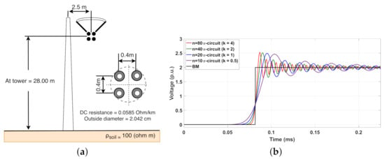
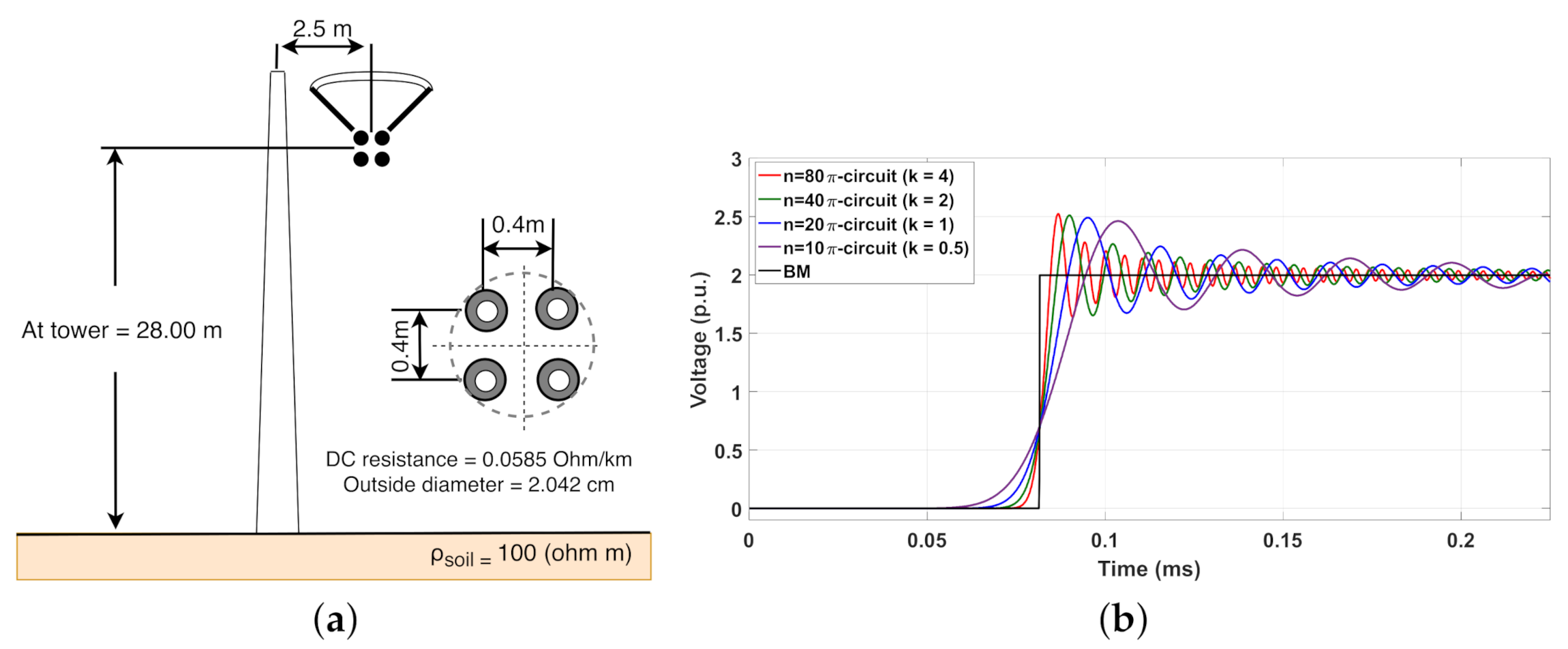
The voltages and currents along the line can be obtained by any numerical integration method to solve (3). In order to illustrate the influence of k in the transient responses, as well as the NSO peaks, a 20-km single-phase TL is employed, the configuration of which is shown in Figure 1a. In this case, the TL is energized by a 1-p.u. DC voltage source (energization maneuver) with an open-circuit receiving end. The computed line parameters are (at 60 Hz): $R^{\prime }$ = 0.075 $\Omega$/km, $L^{\prime }$ = 1.722 mH/km, $C^{\prime }$ = 9.638 nF/km and $G^{\prime }$ is neglected. The TL is represented by n = 10, 20, 40 and 80 $\pi$-circuits which results in k = 0.5, 1, 2 and 4 $\pi$/km, respectively.

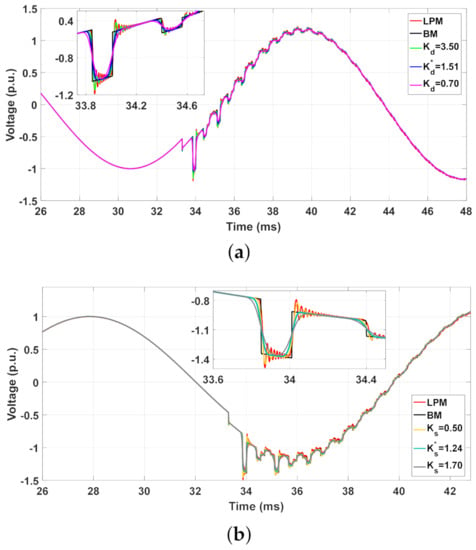
Figure 1. (a) Layout of the single-phase TL; (b) Transient responses obtained by the traditional LPM and BM.

It is adopted that $\Delta$t = 1 μs for these simulations. The transient voltages are calculated by LPM and compared with the responses obtained by BM, as depicted in Figure 1b. It can be noted as k increases, the better is the voltage waveform despite the NSO peaks being more pronounced. As seen, the NSO may exceed by 25% the transient voltage peak for the highest k, which may lead to an erroneous analysis by users. The rise time is better represented as k increases; however, the computational time required to compute the transient responses is higher in comparison with those obtained at lower k. In the next section, modified topologies to mitigate the NSO are presented.

3. Modified Topologies to Mitigate NSO

3.1. LPM with Damping Resistances in the RL Branch

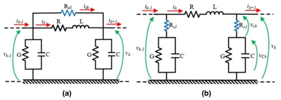
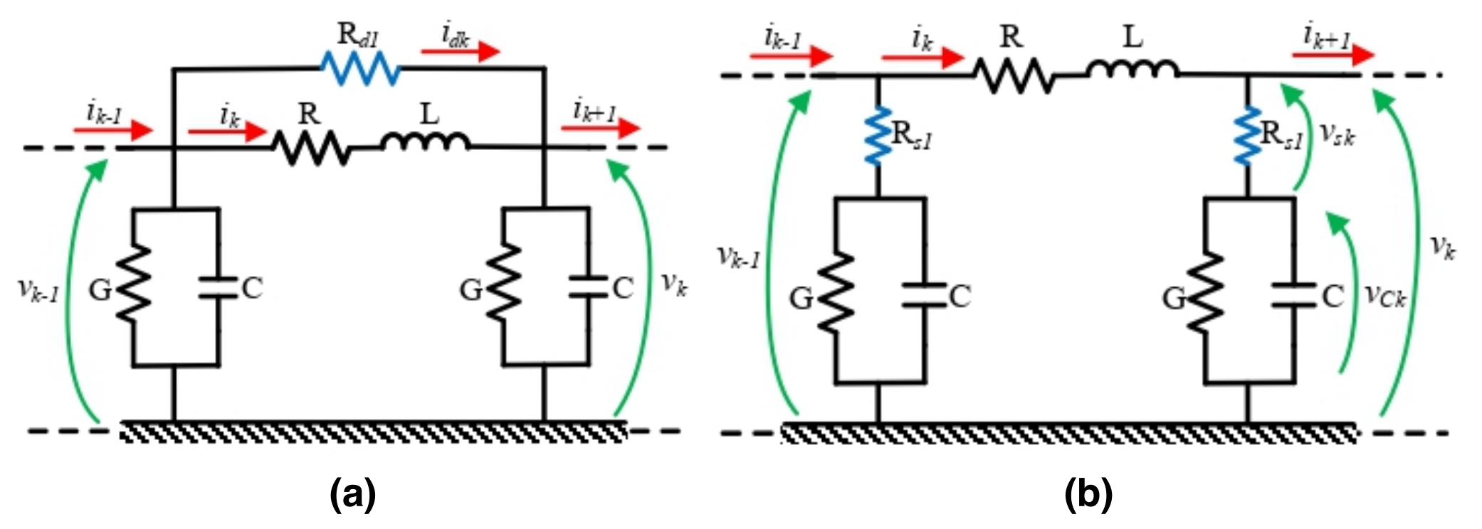
A modified topology ($T_1$) in the literature to mitigate the NSO is presented in Figure 2a [6,20]. To reduce the NSO, a damping resistance R${}_{d1}$ is connected in parallel to the RL branch of the traditional $\pi$-circuit section, as depicted in Figure 2a. In this topology, the artificial damping resistance R${}_{d1}$ and its conductance G${}_{d1}$, are given by:

$$R_{d1}=K_d\frac{2L}{\Delta t},G_{d1}=\frac{1}{R_{d1}}$$

(5)

where K${}_d$ is an adjustable factor that varies between 2 and 10 [6], L is the lumped inductance and $\Delta$t is the step size adopted in the simulations. Applying Kirchhoff’s circuit laws in this modified $\pi$-circuit section, the voltage in the shunt CG branch ($v_k$) and the current in the series RL branch ($i_k$) are written as follows in (Section 3.1).

$$\begin{array}{cc}\hfill \frac{\mathrm{d}{i}_k\left(t\right)}{\mathrm{d}t}& =\frac{-R}{L}{i}_k\left(t\right)+\frac{1}{L}{v}_{k-1}\left(t\right)-\frac{1}{L}{v}_k\left(t\right)\hfill \end{array}$$

(6a)

$$\begin{array}{cc}\hfill \frac{\mathrm{d}{v}_k\left(t\right)}{\mathrm{d}t}& =\frac{1}{C}{i}_k\left(t\right)-\frac{1}{C}{i}_{k+1}\left(t\right)+\frac{G_{d1}}{C}{v}_{k-1}\left(t\right)\hfill \\ \hfill & -\frac{2G_{d1}+G}{C}{v}_k\left(t\right)+\frac{G_{d1}}{C}{v}_{k+1}\left(t\right)\hfill \end{array}$$

(6b)

Figure 2. Modified topologies with: (a) $R_{d1}$ in the $RL$ branch ($T_1$) and (b) $R_{s1}$ in the $CG$ branch ($T_2$).

Expanding to a TL represented by n-$\pi$-circuit sections, the generic $v_k\left(t\right)$ and $i_k\left(t\right)$ are expressed as a linear system of space-state variables, as follows:

$${\dot{\mathit{x}}}_{\mathbf{1}}\left(t\right)={\mathit{A}}_{\mathbf{1}}{\mathit{x}}_{\mathbf{1}}\left(t\right)+{\mathit{B}}_{\mathbf{1}}\mathit{u}\left(t\right)$$

(7)

The matrices ${\mathit{A}}_{\mathbf{1}}$ and ${\mathit{B}}_{\mathbf{1}}$ in (7), and vector ${\mathit{x}}_{\mathbf{1}}$(t) are expressed by:

$$\begin{array}{cc}\hfill {\mathit{A}}_{\mathbf{1}}& =\left[\begin{array}{cc}{\mathit{A}}_{\mathbf{11}}^{\mathbf{1}}& {\mathit{A}}_{\mathbf{12}}^{\mathbf{1}}\\ {\mathit{A}}_{\mathbf{21}}^{\mathbf{1}}& {\mathit{A}}_{\mathbf{22}}^{\mathbf{1}}\end{array}\right]\hfill \end{array}$$

(8a)

$$\begin{array}{cc}\hfill {\mathit{B}}_{\mathbf{1}}& ={\left[\begin{array}{ccccccc}\frac{1}{L}& \cdots & 0& \frac{G_{d1}}{C}& 0& \cdots & 0\end{array}\right]}^T\hfill \end{array}$$

(8b)

$$\begin{array}{cc}\hfill {\mathit{x}}_{\mathbf{1}}\left(t\right)& ={\left[\begin{array}{cccccc}{i}_1\left(t\right)& \cdots & i_n\left(t\right)& v_1\left(t\right)& \cdots & v_n\left(t\right)\end{array}\right]}^T\hfill \end{array}$$

(8c)

3.2. LPM with Damping Resistances in the $GC$ Branch

The modified topology ($T_2$) is depicted in Figure 2b, in which a damping resistance R${}_{s1}$ is inserted in series to the GC branch of the $\pi$-circuit section. The NSO are mitigated with the insertion of a damping resistance R${}_{s1}$ given by:

$$R_{s1}=K_s\frac{\Delta t}{2C}$$

(9)

where C is the lumped shunt capacitance of the $\pi$-circuit, $\Delta$t is the step size of the simulations and the K${}_s$ is an adjustable factor.

Applying the same procedure in Figure 2b, the current ($i_k$) and voltage ($v_k$) are computed as follows:

$$\begin{array}{cc}\hfill \frac{\mathrm{d}{i}_k\left(t\right)}{\mathrm{d}t}& =-\frac{R}{L}{i}_k\left(t\right)+\frac{1}{L}{v}_{k-1}\left(t\right)-\frac{1}{L}{v}_k\left(t\right)\hfill \end{array}$$

(10a)

$$\begin{array}{cc}\hfill \frac{\mathrm{d}{v}_k\left(t\right)}{\mathrm{d}t}& =\left(\frac{1}{C}+{\alpha }_2\right)i_k\left(t\right)-{\alpha }_2{i}_{k-1}\left(t\right)\hfill \\ \hfill & +{\beta }_2{v}_k\left(t\right)+\frac{R_{s1}}{L}{v}_{k+1}\left(t\right)\hfill \end{array}$$

(10b)

where ${\alpha }_2$ and ${\beta }_2$ are defined by (11).

$$\begin{array}{cc}\hfill {\alpha }_2& =\frac{G{R}_{s1}}{C}-\frac{R{R}_{s1}}{L};{\beta }_2=-\frac{G}{C}-\frac{2R_{s1}}{L}\hfill \end{array}$$

(11)

The voltages $v_k\left(t\right)$ and currents $i_k\left(t\right)$ are written in a state-equation form, given by:

$${\dot{\mathit{x}}}_{\mathbf{2}}\left(t\right)={\mathit{A}}_{\mathbf{2}}{\mathit{x}}_{\mathbf{2}}\left(t\right)+{\mathit{B}}_{\mathbf{2}}{\mathit{u}}_{\mathbf{2}}\left(t\right)$$

(12)

where the matrices ${\mathit{A}}_{\mathbf{2}}$ and ${\mathit{B}}_{\mathbf{2}}$ and vector ${\mathit{x}}_{\mathbf{2}}$(t) are given by (Section 3.2).

$$\begin{array}{cc}\hfill {\mathit{A}}_{\mathbf{2}}& =\left[\begin{array}{cc}{\mathit{A}}_{\mathbf{11}}^{\mathbf{2}}& {\mathit{A}}_{\mathbf{12}}^{\mathbf{2}}\\ {\mathit{A}}_{\mathbf{21}}^{\mathbf{2}}& {\mathit{A}}_{\mathbf{22}}^{\mathbf{2}}\end{array}\right]\hfill \end{array}$$

(13a)

$$\begin{array}{cc}\hfill {\mathit{B}}_{\mathbf{2}}& ={\left[\begin{array}{cccccc}\frac{1}{L}& \cdots & 0& \frac{R_{s1}}{L}& \cdots & 0\end{array}\right]}^T\hfill \end{array}$$

(13b)

$$\begin{array}{cc}\hfill {\mathit{x}}_{\mathbf{2}}\left(t\right)& ={\left[\begin{array}{cccccc}{i}_1\left(t\right)& \cdots & i_n\left(t\right)& v_1\left(t\right)& \cdots & v_n\left(t\right)\end{array}\right]}^T\hfill \end{array}$$

(13c)

Although these two modified topologies are known, just a few papers dealing with the influence of these adjustable factors on the reduction of the NSO are presented in the literature [6]. It is worth mentioning that the adjustable factors K${}_s$ and K${}_d$ are selected randomly by the users which may affect significantly the NSO peaks and the rise/fall times in the transient responses. To find the best benefit concerning NSO peaks and distortion at the rise/fall times, a proposed methodology to select the best adjustable factors $K_s^{*}$ and $K_d^{*}$ is presented in this work.

4. Optimization of the Adjustable Factors

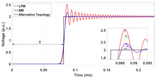
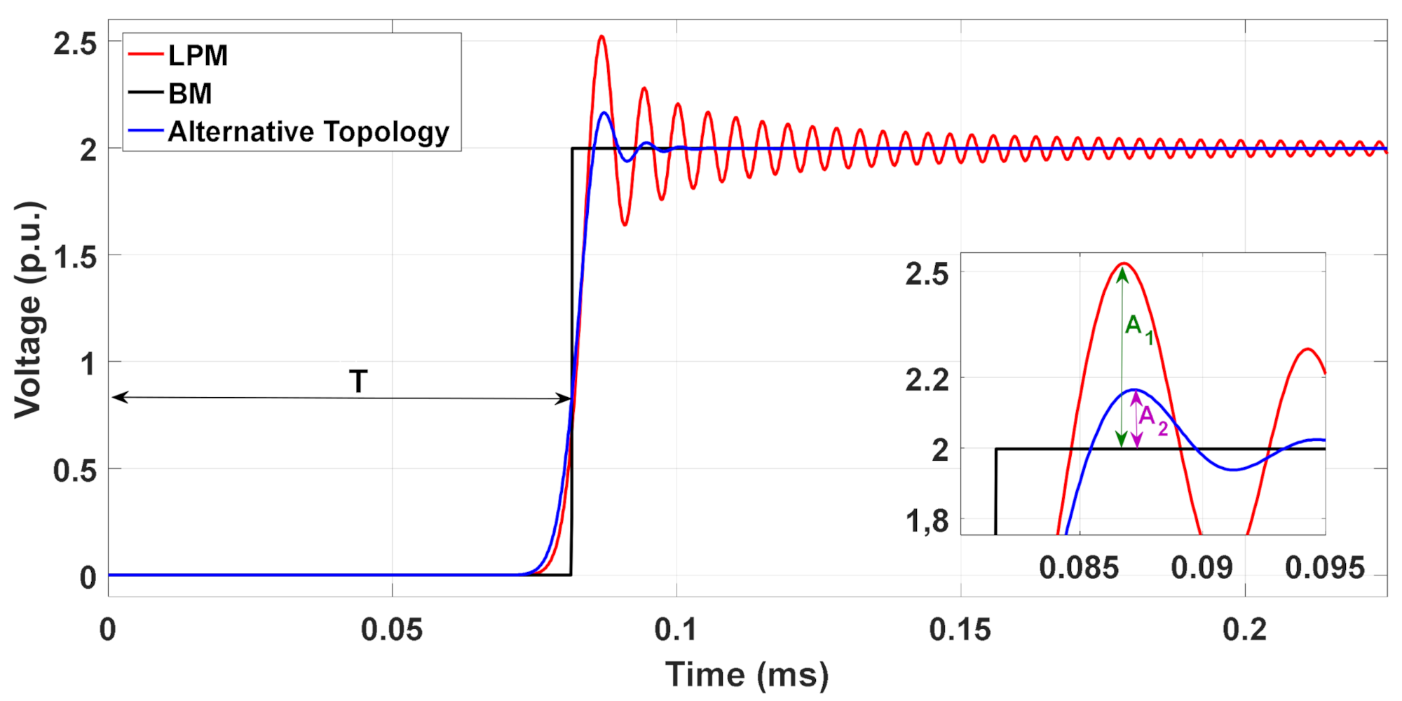
To minimize the peaks of the NSO in the transient responses, the best (optimum) adjustable factors must be computed based on the TL parameters and step size. The optimum adjustable factors are indicated by (*), as $K_d^{*}$ and $K_s^{*}$ in this work. For this purpose, two algorithms are presented to compute the $K_d^{*}$ and $K_s^{*}$, based on the voltage peaks calculated in each topology. To illustrate these optimization methods, the 20-km single-phase TL from Figure 1a is represented by the traditional LPM and by the alternative topologies, which can be the modified $T_1$ or $T_2$. This TL is energized by a 1-p.u. DC voltage source and the receiving end is left open. The computed voltages are illustrated in Figure 3.

Figure 3. Voltages with different TL modeling.

As noted in Figure 3, the NSO in the transient responses obtained with the alternative topology are significantly mitigated in comparison with those computed with the LPM and also closer to those obtained with BM. Aiming to obtain the optimum adjustable factors $K_d^{*}$ and $K_s^{*}$, the amplitudes of the voltage peaks must satisfy the condition in (14), as follows:

$$A_2\le 0.05A_1$$

(14)

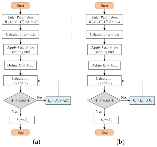
where $A_1$ and $A_2$ are the peaks of the transient voltages obtained for the LPM and modified topology in relation to BM, as detailed in Figure 3. The steps of the optimization algorithm are shown in the flow-chart depicted in Figure 4.

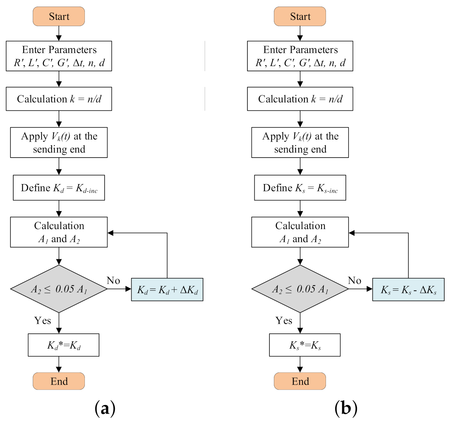
Figure 4. Flow-chart to obtain the optimum adjustable factors: (a) $K_d^{*}$ and (b) $K_s^{*}$.

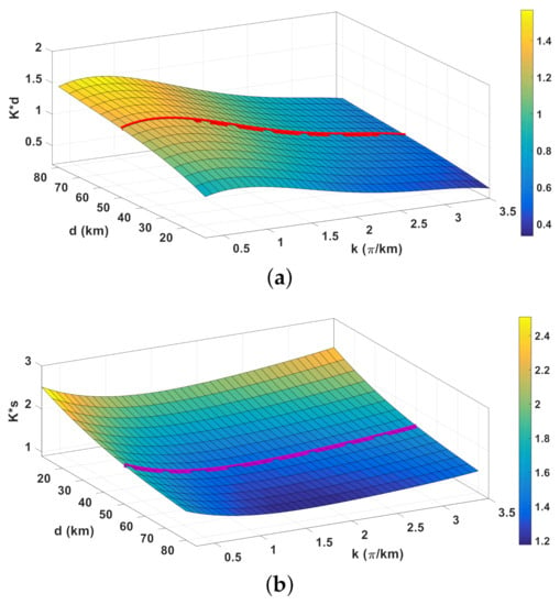
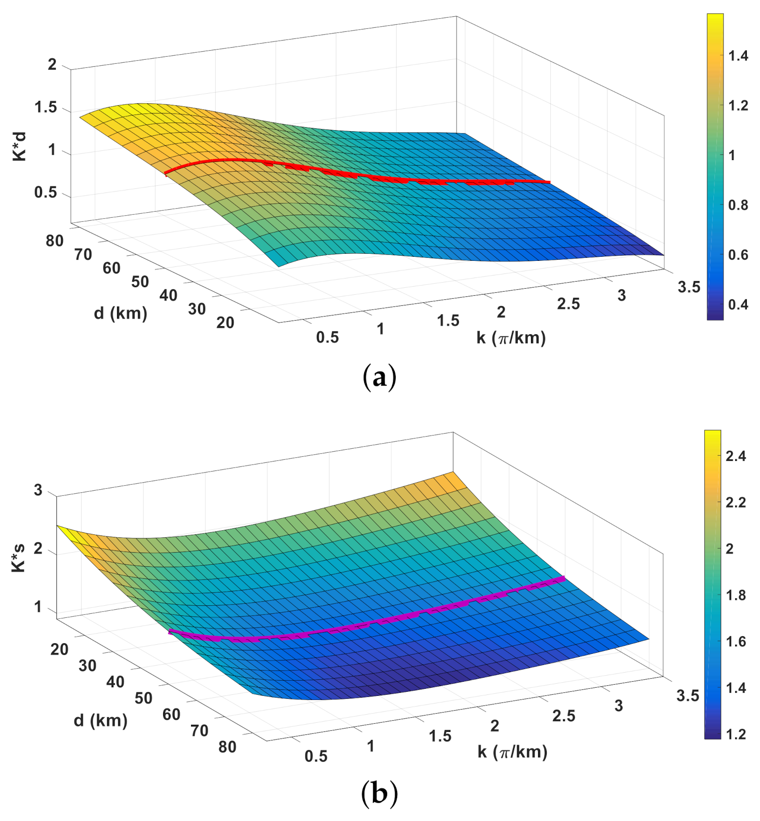
In these algorithms, the $R^{\prime },L^{\prime },C^{\prime }$ and $G^{\prime }$ are the TL per-unit-length parameters, d is the line length, and $\Delta$t is the step time. As a numerical example, the single-phase TL from Figure 1a is represented by several discretization factors k varying from 0.5 up to 3.50 $\pi$-circuits/km and line lengths d varying from 20 up to 80 km where the 3-D graphs (abacuses) are shown in Figure 5. Based on the flow-chart in Figure 4a, the $K_d^{*}$ in a 3-D graph is depicted in Figure 5a. The red curve represents the $K_d^{*}$s for a line of 50-km and varies from 0.3 up to 1.5. For low values of k, the $K_d^{*}$s are high due to the NSO peaks that increase as k increases in the traditional LPM (see Figure 1b). As a consequence, the $K_d^{*}$ tends to decrease, resulting in a lower damping resistance $R_{d1}$ and in a higher reduction in the NSO peaks (as seen in Figure 7 in [6]). However, based on Figure 4b, the $K_s^{*}$ in a 3-D graph is illustrated in Figure 5b. The points along the purple line represent a TL of 50-km obtained for different k ($\pi$/km), in which the $K_s^{*}$ varies from 1.20 up to 2.50. As k increases, the optimum $K_s^{*}$ also increases which reflects on the damping resistances $R_{s1}$ and NSO peaks which are more reduced. In an effort to find an analytical representation of these abacuses, using the Toolbox Curve Fitting in MatLab™, fitted equations for each 3-D surface $K_s^{*}$ and $K_d^{*}$ in Figure 5 are generated, given by a general polynomial form as follows:

$$K^{*}(k,d)=\sum _{i=0}^N\sum _{j=0}^M{P}_{ij}{k}^i{d}^j$$

(15)

where $P_{ij}$ are coefficients for the optimum adjustable factors $K_s^{*}$ and $K_d^{*}$. The $P_{ij}$ for $K_d^{*}$ and $K_s^{*}$ are shown in Table 1 and Table 2, respectively. In both fitted polynomial equations of this work, N = 4 and M = 3.

Figure 5. 3-D Graphs of the optimum adjustable factors as a function of line length and k: (a) $K_d^{*}$ and (b) $K_s^{*}$.

Table 1. Coefficients $P_{ij}$ of the $K_d^{*}$.

		${\mathit{P}}_{\mathit{ij}}$
(i, j)	0	1	2	3
0	0.972	0.147	−0.033	0.011
1	−0.402	−0.058	0.008	−0.003
2	0.094	−0.013	0.003	0
3	0.086	0.017	0	0
4	−0.055	0	0	0

Table 2. Coefficients $P_{ij}$ for the $K_s^{*}$.

		${\mathit{P}}_{\mathit{ij}}$
(i, j)	0	1	2	3
0	0.049	−0.125	0.029	−0.006
1	0.049	−0.004	0	−0.001
2	0.103	−0.013	0.002	0
3	−0.059	0.005	0	0
4	0.019	0	0	0

Interface with ATP Software

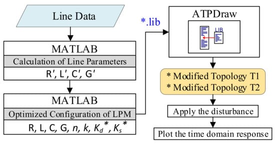
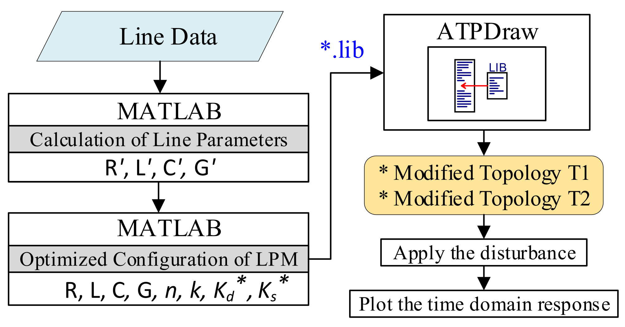
As depicted in the Figure 6, an alternative to simulate the modified topologies of the LPM consist of employing the programing language MatLab combined with ATPDraw. In this case, using a programing code in MatLab, the per-unit-length line parameters (R’, L’, C’and G’) are calculated for a single-phase line. Then, using the steps described in the flow-chart from Figure 5, the optimized topology using the damping adjustable factor (Kd* or Ks*), the number of $\pi$-circuits (n) and the discretization factor (k) are selected. An external code is applied to save these parameters (R’, L’, C’, G’, n, k, Kd* and Ks*), that will represent a line with a file in the format *.lib, as described in [21]. Finally, this *.lib file is loaded in the LIB icon in ATPDraw which will generate the modified topologies $T_1$ and $T_2$ that represent the transmission line. The user chooses the type of disturbance applied at the receiving end (such as the amplitude of the voltage for the energization maneuver) and the transient responses are computed directly in the time domain.

Figure 6. Flow-chart to compute the transient responses with the modified topologies using ATPDraw software.

5. Numerical Results and Discussions

The numerical results are divided into three sections organized as follows: in Section 5.1, the frequency responses of the modified topologies are compared to those obtained by the traditional LPM. In Section 5.2, the transient responses are computed for three scenarios in single-phase TLs. In Section 5.3, transient responses are computed for two scenarios using three-phase TLs. Due to the low-frequency range of the switching maneuver, the line parameters are considered constants for this study. The numerical method of Heun is adopted to solve all the state equations of each topology.

5.1. Frequency Responses for the TL Models

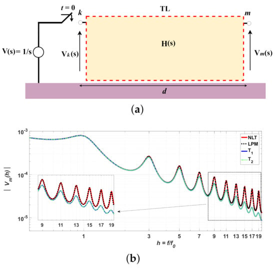
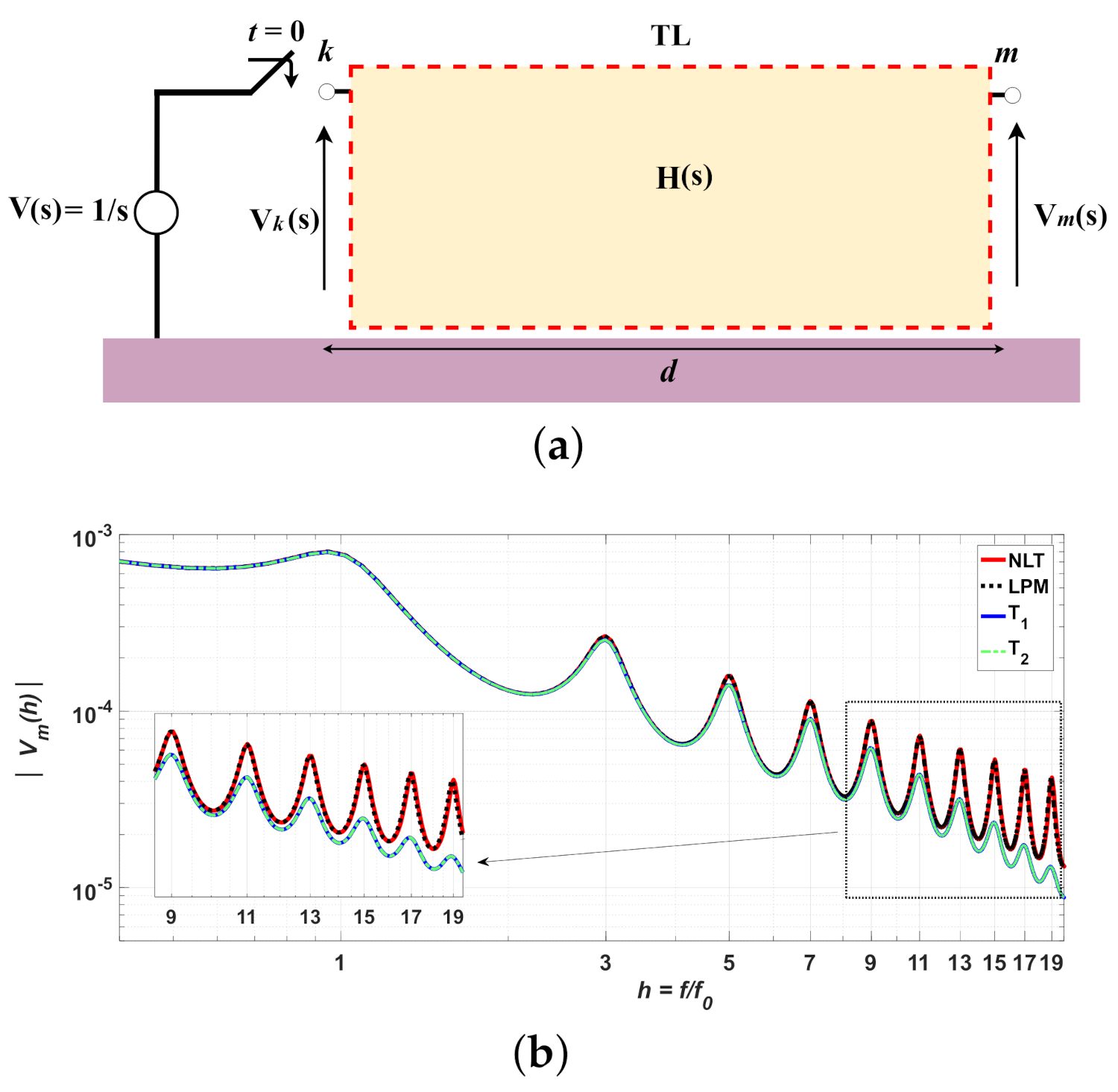
The single-phase TL is employed to calculate the frequency response of the transient voltages $V_m$(s) at the open receiving end. For these simulations, a 1-p.u. DC voltage source is applied at t = 0 s at the sending end and the transient voltages are obtained with the traditional LPM and modified topologies $T_1$ and $T_2$. Figure 7a shows a black-box model for transfer function H(s) represented for each previous topology. This transfer function is given by:

$$H\left(s\right)=\frac{V_m\left(s\right)}{V_k\left(s\right)}$$

(16)

where $V_k($s) and $V_m($s) are voltages at the sending and receiving ends in the frequency domain and s = $j\omega$ is the complex angular frequency (rad/s). To clarify the results, the abscissa is normalized by the fundamental $f_0$ and harmonic $f_h$ frequencies expressed by [6,22]:

$$f_0=\frac{1}{4\tau }=\frac{1}{4d\sqrt{L^{\prime }{C}^{\prime }}};f_h=(2m+1)f_0$$

(17)

where $\tau$ is the traveling time, L’ and C’ are the p.u.l. inductance and capacitance and d is the line length. The frequency response is calculated for the TL length of 20-km depicted in Figure 7a. This line is represented by the traditional LPM with k = 3 $\pi$/km and p.u.l. parameters of $R^{\prime }$ = 0.075 $\Omega$/km, $L^{\prime }$= 1.722 mH/km, $C^{\prime }$= 9.638 nF/km and $G^{\prime }$ neglected. The TL represented by the modified topologies $T_1$ and $T_2$, using fitted Equations (15) and 3-D abacus in Figure 5, present optimum adjustable factors of $K_d^{*}$ = 0.526 and $K_s^{*}$ = 1.943. The computed fundamental frequency f${}_0$ is approximately 3068 Hz. The receiving-end voltage $V_m$(s) is computed by a step function $V_k$(s) = 1/s applied at the sending end. The computed $V_m$(s) as a function of the normalized h = $f_h$/$f_0$ is illustrated in Figure 7b where $f_h$ is the harmonic frequency given in (17), for m integer. The transient peaks occur at the odd harmonic frequencies (h) such as: 1$f_0$≈ 3068 Hz, $f_3$≈ 9204 Hz, $f_5$≈ 15,304 Hz and so on. It can be observed that the voltage peaks for $T_1$ and $T_2$ topologies present lower values in comparison with those obtained by the LPM as the harmonic frequency increases. As a consequence, the peaks of the transient responses will have a pronounced reduction in the NSO when these modified topologies are used (further presented). The harmonic peaks of the $H\left(s\right)$ are lower than those computed with the LPM and BM, for a given harmonic frequency, which represents an expressive attenuation in the time-domain responses.

Figure 7. (a) Black-box TL modeled by H(s); (b) Magnitude of $V_m($s) for the LPM, BM, $T_1$ and $T_2$.

5.2. Performance of the Modified Topologies

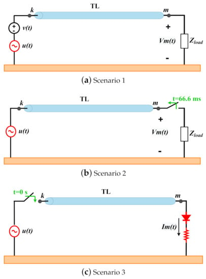
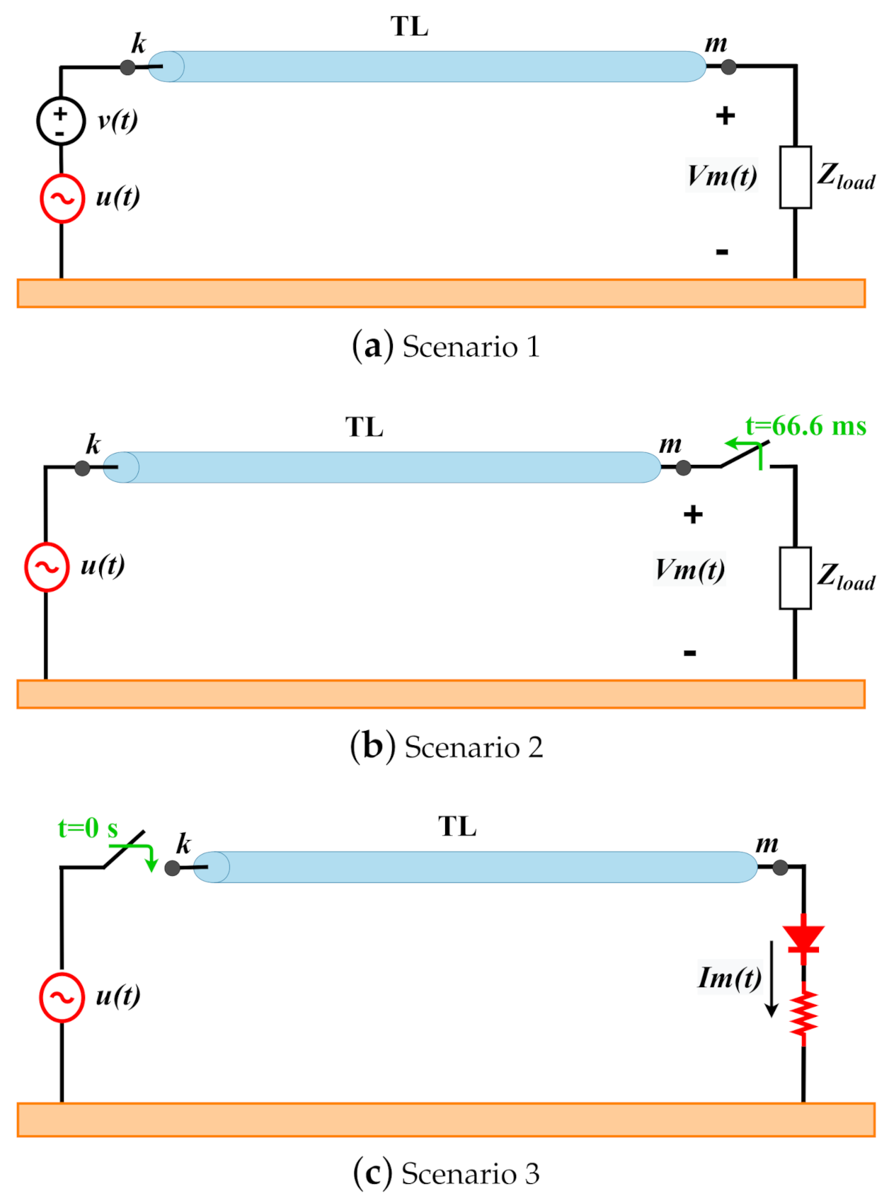
To investigate the performance in the transient responses with optimum adjustable factors in the modified topologies, single-phase TLs are represented by the traditional LPM and modified topologies $T_1$ and $T_2$ in three distinct scenarios, as depicted in Figure 8. The transient responses are compared with those obtained with the classical BM [18,23]. The TL parameters are: $R^{\prime }$ = 0.075 $\Omega$/km, $L^{\prime }$ = 1.722 mH/km, $C^{\prime }$ = 9.638 nF/km and $G^{\prime }$ is neglected. The three scenarios studied are:

Figure 8. Single-phase TLs studied in an: (a) open-circuit test, (b) load rejection test and (c) nonlinear load test.

(a)

Scenario 1: The TL is energized by a 1-p.u./60-Hz voltage source $u\left(t\right)$ and a load is connected in the receiving end ($Z_{load}$ = 6000 $\Omega$). The transient voltage $V_m$(t) is computed when an impulsive source $v\left(t\right)$ = 0.15 p.u. and is shortly inserted at the sending end at t = 0.5 s ramp-up time, generating the second group of transients;

(b)

Scenario 2: The TL is energized by a 1- p.u./60-Hz voltage source $u\left(t\right)$ and ($Z_{load}$ = 2000 $\Omega$) is connected. At t = 66.66 ms, the load switch is opened (load rejection) and the transient voltage is generated;

(c)

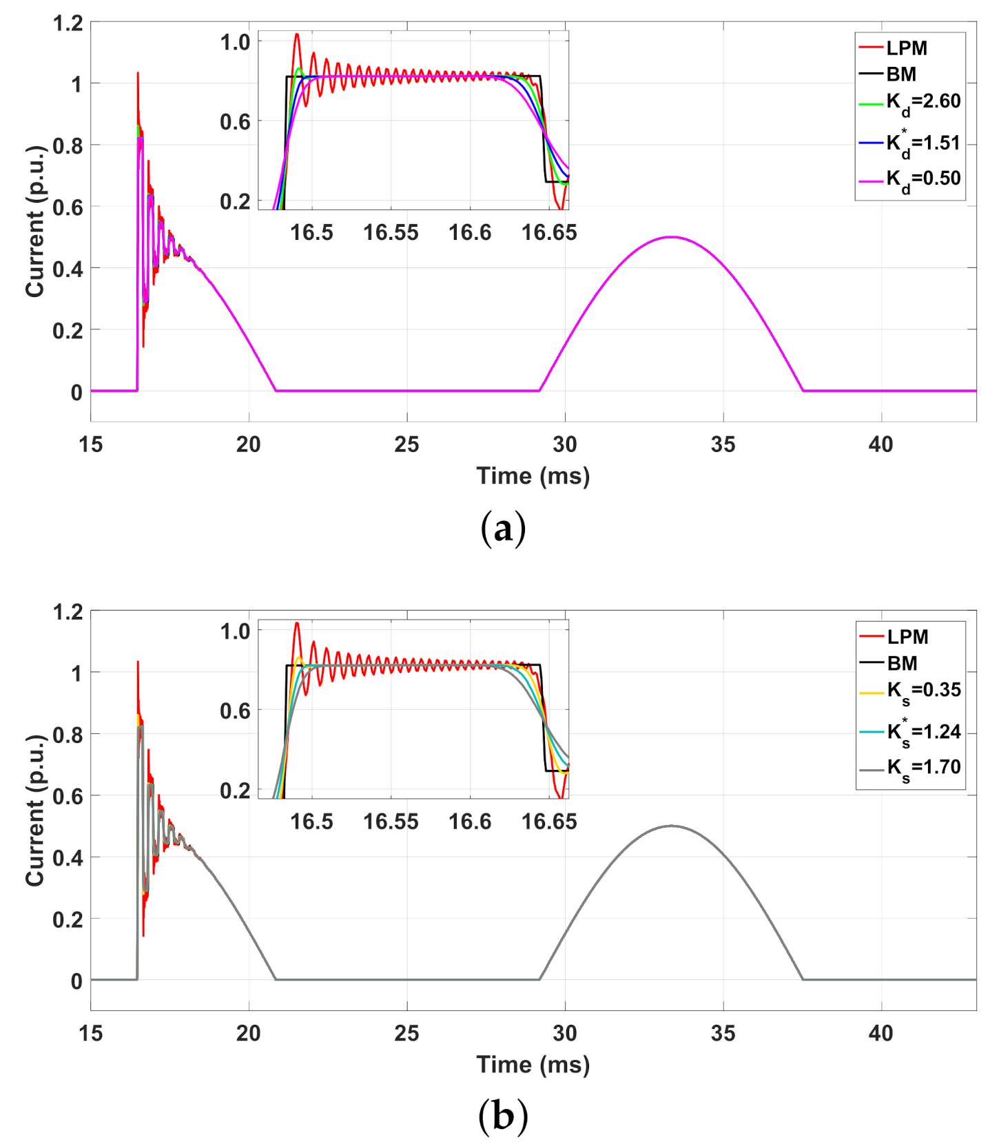
Scenario 3: The TL is energized by a 1-p.u./60-Hz voltage source $u\left(t\right)$ and a nonlinear load (ideal diode and $Z_{load}$ = 2000 $\Omega$) is connected where the transient current $I_m$(t) is computed.

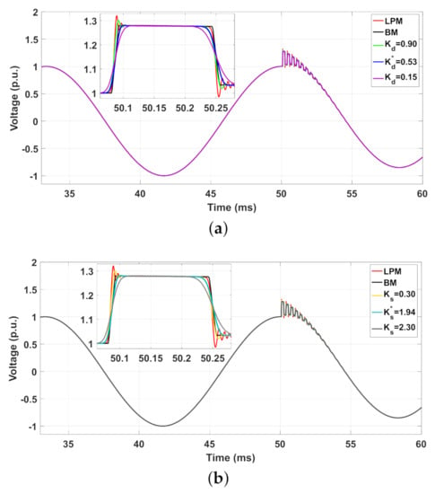
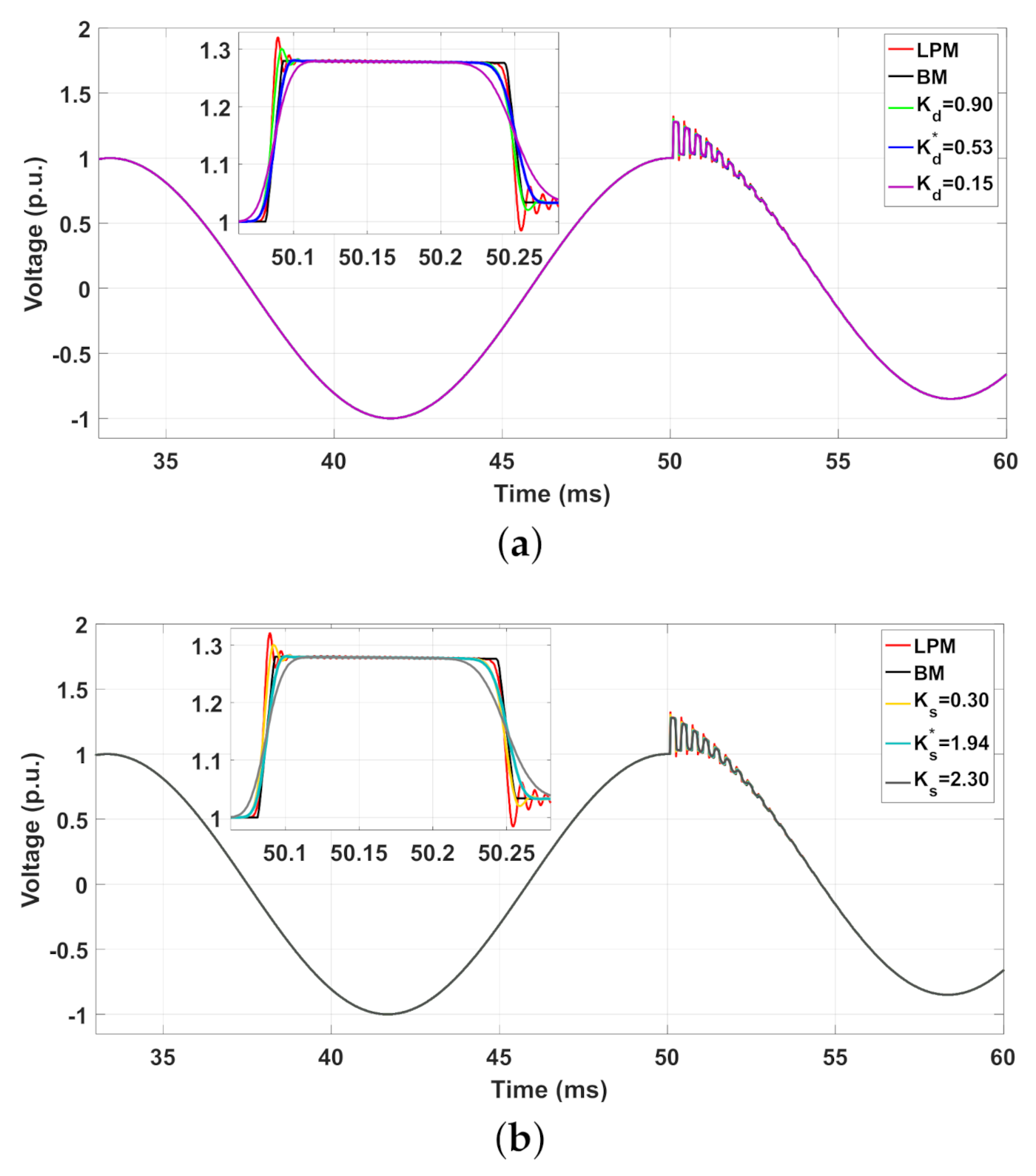
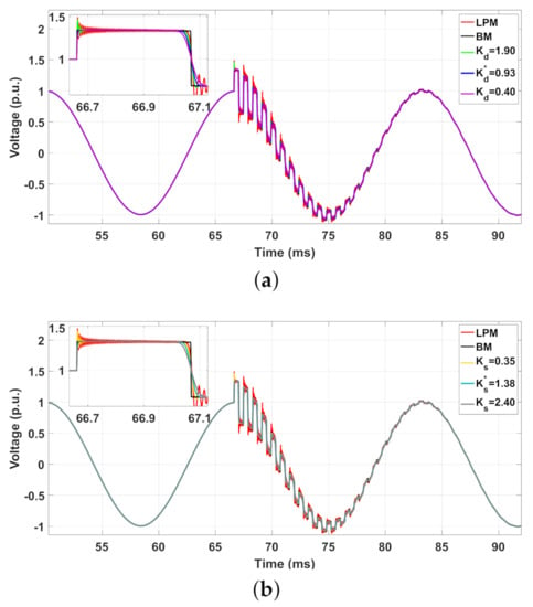
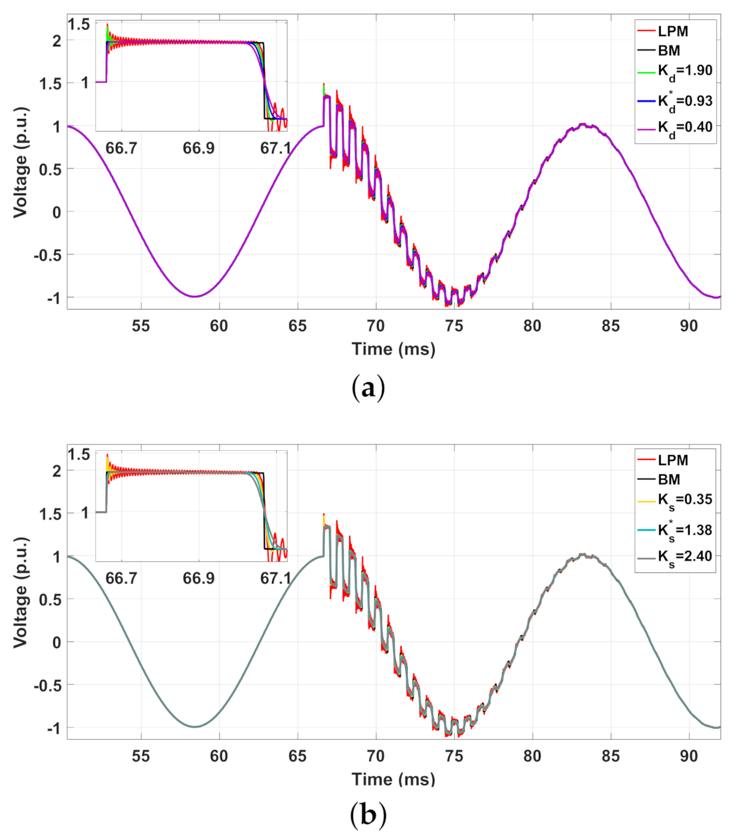
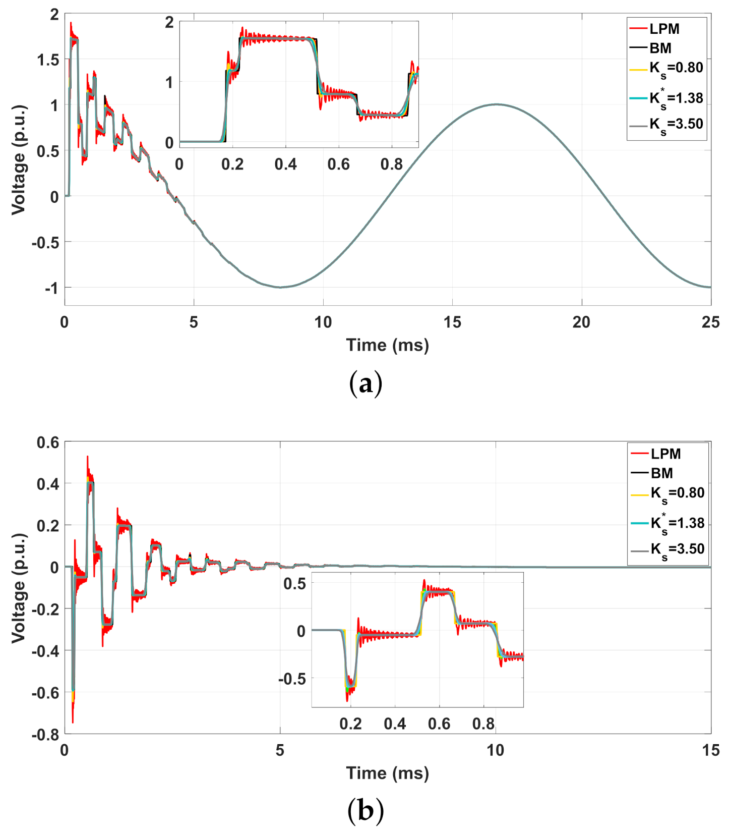
In each scenario, a given line length d and discretization factor k are chosen. Based on Equation (15) and on Figure 5, the optimum adjustable factors are calculated and these values are organized in Table 3. Other values of $K_d$ and $K_s$ are employed to compute the transient responses which are described in each correspondent figure. The simulated responses obtained in the scenarios 1, 2 and 3 are illustrated in Figure 9, Figure 10 and Figure 11, respectively. As seen in these figures, the NSO are significantly mitigated when the modified topologies are employed; however, high distortions in the rise and fall times are associated for each topology. In comparison with the responses for random factors $K_d$ and $K_s$, the responses with the maximum attenuation and minimum distortion are obtained for optimum adjustable factors $K_d^{*}$ and $K_s^{*}$ in each of the modified topologies ($T_1$) and ($T_2$).

Table 3. Parameters in the three scenarios studied.

	Length d (km)	k ($\mathit{\pi }$/km)	Topology	Opt. Factors Equation (17)
Scenario 1	20	3	$T_1$	$K_d^{*}$ = 0.526
	20	3	$T_2$	$K_s^{*}$ = 1.943
Scenario 2	50	2	$T_1$	$K_d^{*}$ = 0.929
	50	2	$T_2$	$K_s^{*}$ = 1.375
Scenario 3	80	1	$T_1$	$K_d^{*}$ = 1.510
	80	1	$T_2$	$K_s^{*}$ = 1.236

Figure 9. $V_m\left(t\right)$ for the 20-km single-phase TL in scenario 1 for: (a) LPM, BM and $T_1$ and (b) LPM, BM and $T_2$.

Figure 10. $V_m\left(t\right)$ for the 50-km single-phase TL in scenario 2: (a) LPM, BM and $T_1$ and (b) LPM, BM and $T_2$.

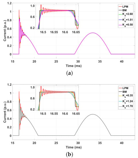
Figure 11. $I_m\left(t\right)$ for the 80-km single-phase TL in scenario 3: (a) LPM, BM and $T_1$ and (b) LPM, BM and $T_2$.

The transient responses obtained with the $K_d^{*}$ and $K_s^{*}$ are in good agreement with those responses obtained by BM, assumed here as a reference. To verify the performance of the modified topologies, the percentage error $ϵ$(%) obtained with the LPM and with the modified topologies $T_1$ and $T_2$ are computed for each scenario. The percentage error $ϵ$(%) is given by

$$ϵ(\%)=\frac{|R_{BM}-R_{mod-top}|}{|R_{BM}|}\times 100\%,$$

(18)

where R represents the transient response (voltage or current) and the index $mod-top$ is the transient response for each modified topology. The peaks P (p.u.) of each transient response and $ϵ$(%) obtained in the scenarios 1, 2 and 3, are organized in Table 4. It can be seen in this table, the response peaks computed with topologies $T_1$ and $T_2$ using the optimum $K_d^{*}$ and $K_s^{*}$ have provided the highest reduction in the NSO, resulting in the lowest percentage errors, as highlighted in light-green. These errors are lower than 1% in comparison with those calculated with the LPM, which gave errors of 3.20%, 11% and 26% as noted in Table 4. These numerical results confirm that the best agreement is obtained with the optimum adjustable factors $K_d^{*}$ and $K_s^{*}$ for the topologies $T_1$ and $T_2$, respectively. In the next section, transient voltages are analyzed for the three-phase TLs under two different scenarios.

Table 4. Transient Peaks (P) and Errors ($ϵ$(%)) for scenarios 1, 2 and 3.

	Scenario 1		Scenario 2			Scenario 3
Model	P(p.u.)	$\mathit{ϵ}$(%)	Model	P(p.u.)	$\mathit{ϵ}$(%)	Model	P(p.u.)	$\mathit{ϵ}$(%)
BM (ref)	1.279	–	BM	1.339	–	BM	0.820	–
LPM	1.320	3.20	LPM	1.489	11.202	LPM	1.034	26.08
$T_1$/$K_d$ = 0.90	1.303	1.88	$K_d$ = 1.90	1.461	9.11	$K_d$ = 2.60	0.875	6.718
$T_1$/$K_d$ = 0.15	1.265	1.09	$K_d$ = 0.40	1.425	6.43	$K_d$ = 0.50	0.783	4.511
$T_1$/$K_d^{*}$ = 0.53	1.280	0.07	$K_d^{*}$ = 0.93	1.337	0.149	$K_d^{*}$ = 1.51	0.821	0.123
$T_2$/$K_s$ = 0.30	1.201	1.49	$K_s$ = 0.35	1.420	6.5	$K_s$ = 0.35	0.792	3.417
$T_2$/$K_s$ = 2.30	1.305	2.03	$K_s$ = 2.40	1.452	8.442	$K_s$ = 1.70	0.856	4.390
$T_2$/$K_s^{*}$ = 1.54	1.281	0.16	$K_s^{*}$ = 1.38	1.338	0.075	$K_s^{*}$ = 1.24	0.822	0.245

5.3. Modified Topologies in Three-Phase Lines

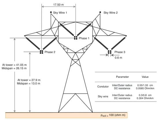
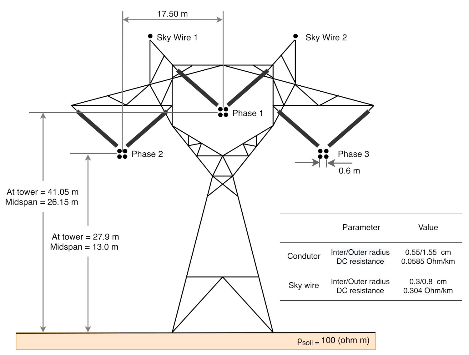
To extend the validation of the modified topologies for transients, the transient responses for a 50-km and 80-km three-phase TL are carried out, where modal decomposition technique is applied in each TL [24]. In this technique, a transformation matrix decouples a three-phase transmission line into three distinct single-phase lines (or propagation modes) where each one is represented by the traditional LPM and modified $T_1$ and $T_2$ topologies [25]. In this work, the Clarke’s matrix is employed to decouple the three-phase TLs. Once the transient responses are obtained for each independent mode, they are converted to a phase domain employing inverse Clarke’s matrix transformation. The ideally transposed three-phase TL is composed of bundles of 0.6-m quad-conductor per phase (phases 1, 2 and 3) plus two ground-wire conductors are installed. The spacing, including average conductor sag relative to the center of the tower and tower dimensions, are shown in Figure 12. The soil resistivity is ${\rho }_e$ = 100 $\Omega$m, relative permittivity ${\epsilon }_r$ = 1, and the ground-return impedances are computed by the Carson’s approach. The longitudinal impedance and transversal admittance matrices ([Z] ($\Omega$/km) and [Y], ($\mu$S/km), respectively), computed at 60 Hz, are given as follows:

$$\begin{array}{cc}\hfill \left[\mathit{Z}\right]& =\left[\begin{array}{ccc}0.0665+0.4774i& 0.0501+0.1425i& 0.0501+0.1425i\\ 0.0501+0.1425i& 0.0665+0.4774i& 0.0564+0.3890i\\ 0.0501+0.1425i& 0.0501+0.1425i& 0.0665+0.4774i\end{array}\right]\hfill \\ \hfill \left[\mathit{Y}\right]& =\left[\begin{array}{ccc}4.5573i& -0.4435i& -0.4435i\\ -0.4435i& 4.5573i& -0.07318i\\ -0.4435i& -0.4435i& 4.5573i\end{array}\right]\hfill \end{array}$$

Figure 12. Configuration of the three-phase TL.

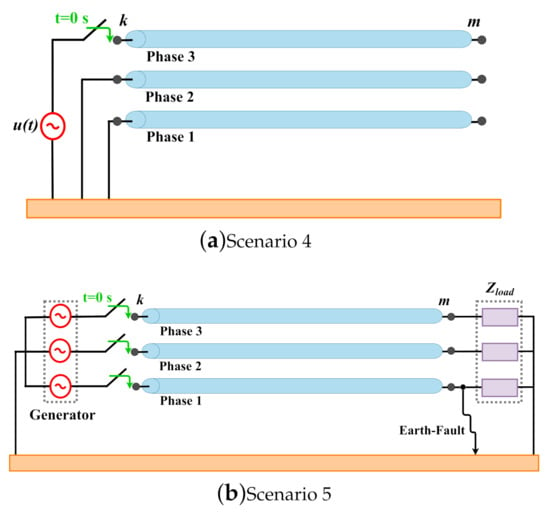
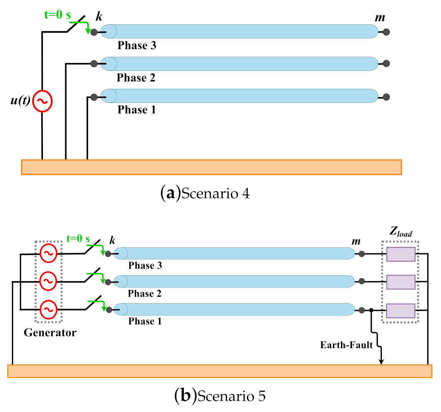
The three-phase TL configuration is provided in Figure 13, where two different scenarios are studied:

Figure 13. Layouts of the three-phase TL for an: (a) open-circuit test; (b) fault test.

(a)

Scenario 4: The 50-km three-phase TL is energized by a 1-p.u./60-Hz voltage source only in phase 1 and the other phases are short-circuited. The receiving end is left open, as depicted in Figure 13a;

(b)

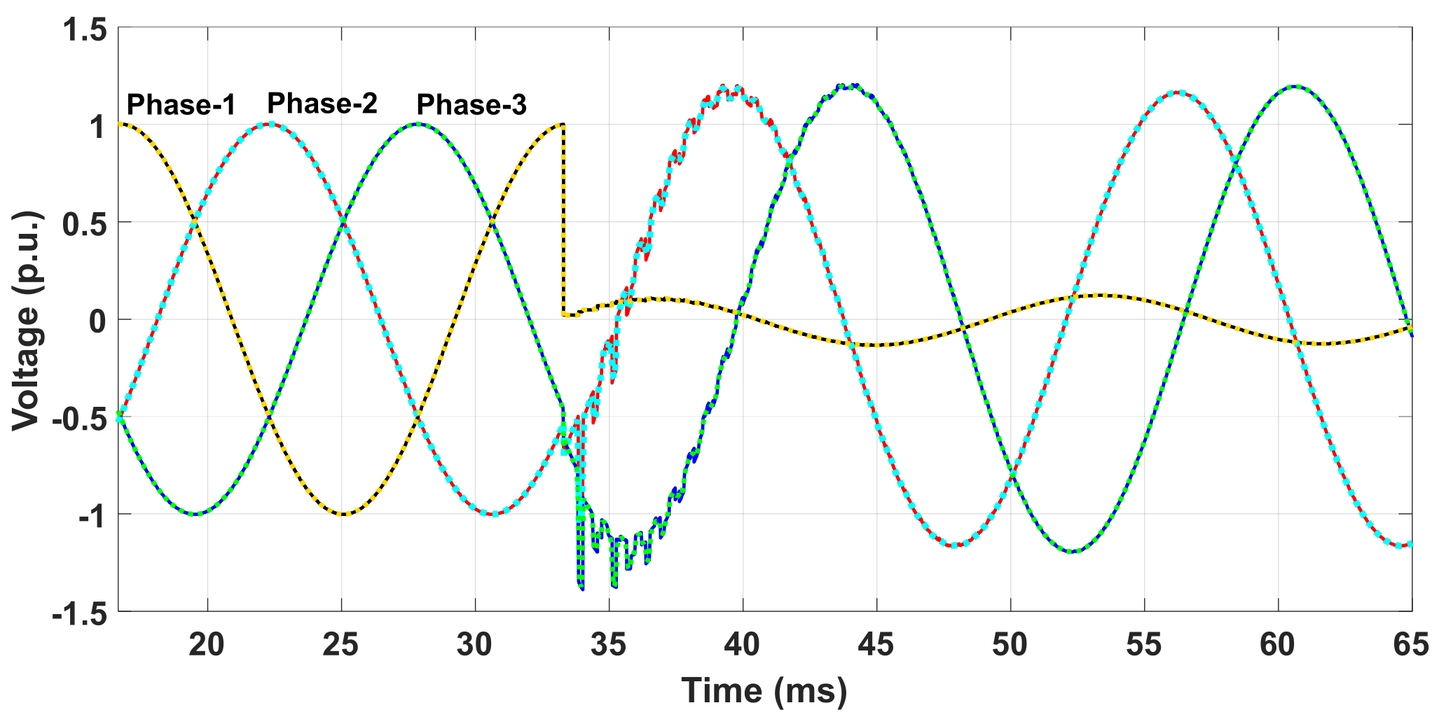
Scenario 5: The 80-km three-phase line is energized by a 1-p.u./60-Hz generator at t = 0 s and a balanced load is connected at the receiving end ($Z_{load}$ = 3 k$\Omega$). At t = 33.33 ms, a fault occurs at phase 1, as depicted in Figure 13b.

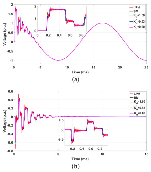
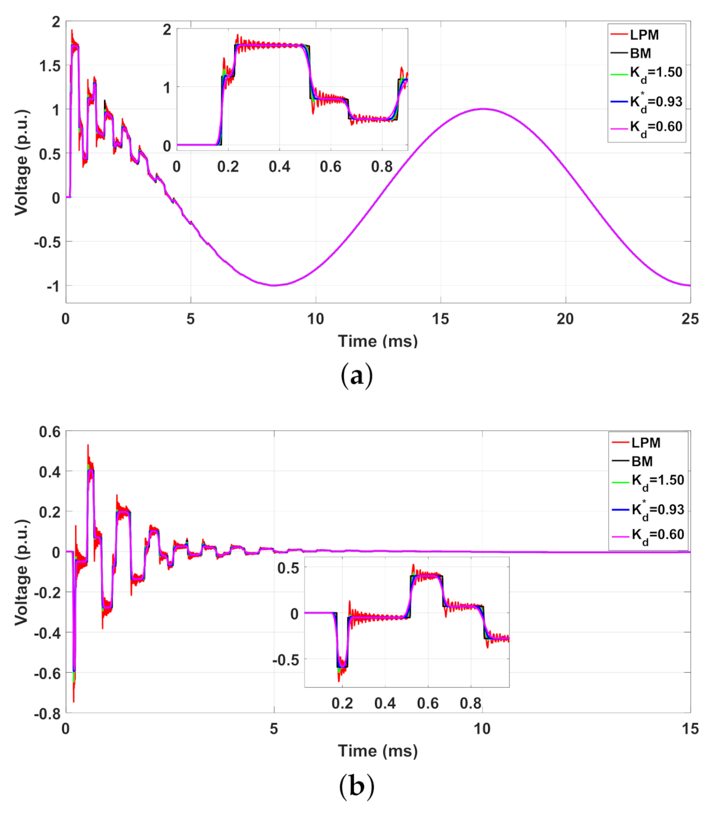
In both scenarios, the transient voltages $V_m$(t) are computed by the traditional LPM and modified topologies $T_1$, $T_2$ with the best adjustable factors $K_d^{*}$ and $K_s^{*}$ and compared with BM. In Scenario 4, the 50-km three-phase TL is decoupled in three single-phase lines represented by k = 2$\pi$/km where the adjustable factors are $K_d^{*}$ = 0.929 and $K_s^{*}$ = 1.375, based on (15). In Scenario 5, the 80-km three-phase TL is decoupled in three single-phase lines represented by k = 1$\pi$/km where the adjustable factors are $K_d^{*}$ = 1.51 and $K_s^{*}$ = 1.236. To verify the mitigation of the NSO, simulation results are compared with transient responses computed by BM. The transient voltages $V_m$(t) for Scenario 4 obtained with $T_1$ are shown in Figure 14 and those obtained with $T_2$ are shown in Figure 15.

Figure 14. $V_m$(t) in Scenario 4 for the LPM, $T_1$ and BM with $K_d^{*}$: (a) Phase 1 (b) Phase 2 (or Phase 3).

Figure 15. $V_m$(t) in Scenario 4 obtained with the LPM, $T_2$ and BM with $K_s^{*}$: (a) Phase 1 (b) Phase 2 (or Phase 3).

The percentage errors $ϵ$(%) based on voltage peaks illustrated in Figure 14 and Figure 15 obtained with the LPM, with the modified topologies $T_1$ and $T_2$ for best adjustable factors and with BM for scenario 4 are shown in Table 5. In Figure 14 and Figure 15, the energization generates surge waves that travel along the line, resulting in overvoltages at the receiving end. Due to the inductive and capacitive couplings between the phases, induced voltages are produced at phases 2 and 3. It can be seen that when a positive variation in the voltage at phase 1 induces negative voltages at phases 2 and 3, as predicted by Faraday’s law. In the steady state, the voltage at phase 1 will reach 1 p.u. while at phases 2 and 3 it is zero, due to the open-circuit condition. In these figures, one observes that the amplitude of NSO is significantly reduced when the three-phase line is represented by the modified topologies $T_1$ and $T_2$. The voltage peaks and errors obtained are shown in Table 5. As noted, for the voltages in phase 1, the errors for the topologies $T_1$ and $T_2$ are equal to 0.82%, whereas the LPM provides an error of 12.64%. In relation to phases 2 and 3, the voltages with the LPM have presented an error of 26.82%, whereas the modified topologies $T_1$ and $T_2$ have provided errors smaller than 1.50%. These results indicate the good performance in the attenuation of NSO, especially, for the induced voltages at phases 2 and 3.

Table 5. Voltage peaks and percentage $ϵ$(%) for scenario 4.

	Voltage Peak (p.u)					$\mathit{ϵ}$ (%)
	BM (ref)	LPM	${\mathit{T}}_{\mathbf{1}}$	${\mathit{T}}_{\mathbf{2}}$		LPM	${\mathit{T}}_{\mathbf{1}}$	${\mathit{T}}_{\mathbf{2}}$
Phase 1	1.709	1.925	1.695	1.695		12.64	0.82	0.82
Phases 2 and 3	−0.589	−0.747	−0.597	−0.595		26.825	1.378	1.019

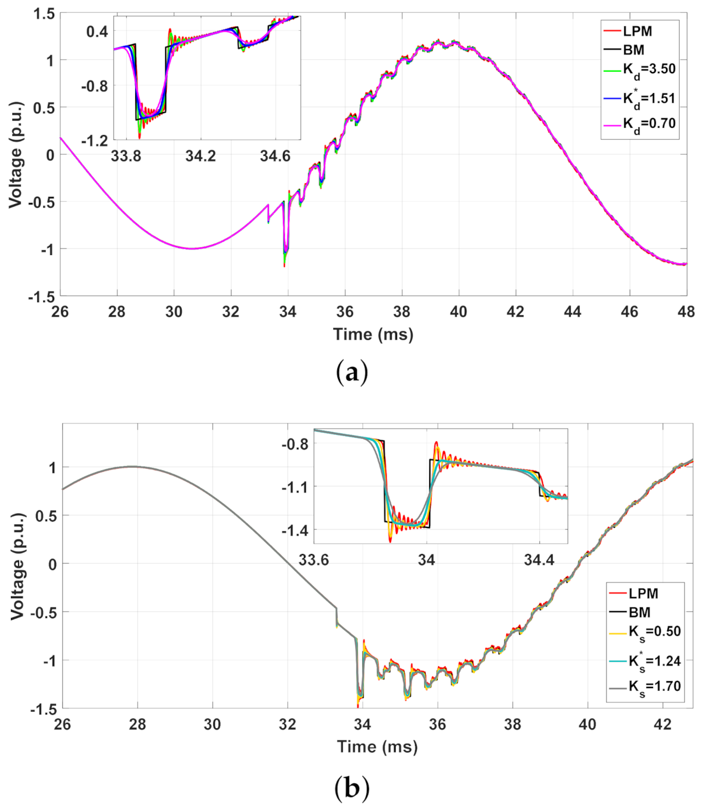
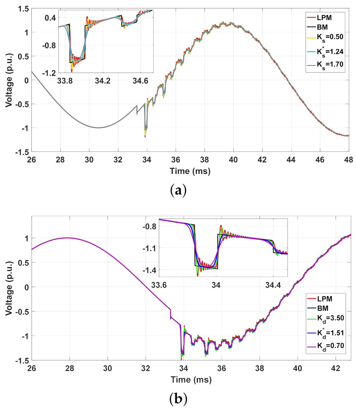
In scenario 5, the transient voltages are generated by the three-phase generator switched on at t = 0 s, and at t = 33 ms an earth-fault occurs at phase 1 at the receiving end (the fault impedance is 5 $\Omega$). The transient voltages at the receiving end $V_m$(t) computed with BM, traditional LPM and modified topologies $T_1$ and $T_2$ are illustrated in Figure 16. In order to highlight the performance of the optimum adjustable factors $K_d$ and $K_s$, the simulations are detailed as depicted in Figure 17 for $T_1$ and Figure 18 for $T_2$, respectively. The transient voltage peaks in Figure 17 and Figure 18, after the earth-fault at t = 33 ms, and the $ϵ$(%) obtained with the LPM, with the modified topologies $T_1$ and $T_2$ for best adjustable factors, and with BM for the scenario 5 are shown in Table 6 (only for phases 2 and 3). Due to the mutual coupling inherent in the three-phase line, the overcurrent in phase 1 produces the transients at the load, where the NSO are presented in the LPM responses. The voltage peaks are shown in Table 6. It can be seen in detailed parts of Figure 17 and Figure 18 that voltage peaks are significantly mitigated in the transient responses when the modified topologies are employed. The errors in phase 2 for the modified topologies $T_1$ and $T_2$ are smaller than 1.50%, whereas the LPM has provided 12.78%. For phase 3, the errors are smaller than 1% and an error of 10.45% is seen for the LPM.

Figure 16. Three-phase TL with an earth-fault in phase 1 at t = 33 ms.

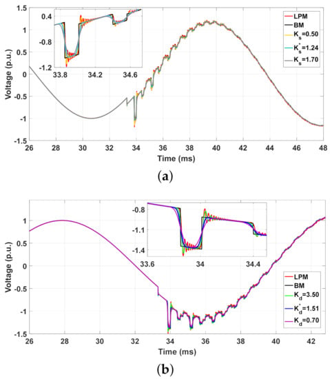
Figure 17. Transient voltages under an earth-fault with LPM, $T_1$ and BM: (a) Phase 2 and (b) Phase 3.

Figure 18. Transient voltages under an earth-fault with LPM, $T_2$ and BM: (a) Phase 2 and (b) Phase 3.

Table 6. Voltage peaks and $ϵ$(%) for each modified topology for scenario 5.

	Voltage Peak (p.u)					$\mathit{ϵ}$ (%)
Phase	BM (ref)	LPM	${\mathit{T}}_{\mathbf{1}}$	${\mathit{T}}_{\mathbf{2}}$		LPM	${\mathit{T}}_{\mathbf{1}}$	${\mathit{T}}_{\mathbf{2}}$
Phase 2	−1.056	−1.191	−1.041	−1.044		12.784	1.421	1.136
Phase 3	−1.349	−1.490	−1.338	−1.334		10.452	0.815	0.964

In general, the modified topologies behave as low-pass filter circuits that mitigate the NSO in the transient responses directly in the time domain and are in good agreement with those transient responses obtained with BM. Furthermore, no digital or analog filters are needed to mitigate the NSO in the computed transient responses when the simulations are carried out with modified topologies. The proposed algorithms are simple tools that can be implemented, and 3-D surfaces with fitted equations are a fast way to calculate the best adjustable factors of each topology. Based on these best adjustable factors, the maximum attenuation of the NSO and minimum distortion in the time-domain transient responses are obtained when low-frequency disturbances occur in TLs. Additionally, these modified topologies are easily incorporated into EMP-type programs.

6. Conclusions

This paper has presented two modified LPM topologies based on the cascaded $\pi$-circuit for the representation of short transmission lines subjected to energization maneuvers and faults, both being low-frequency disturbances common in power systems. Furthermore, to determine the best adjustable factors for the modified topologies, a simple programing code was described in this paper.

The modified topologies have presented interesting behavior regarding the mitigation of spurious oscillations in the simulated transient responses. It was demonstrated that the optimized adjustable factors provide the maximum mitigation in the NSO, especially the peaks, of the obtained transient responses. The adjustable factors $K_d$ and $K_s$ of these modified topologies were randomly selected by the authors in the literature. The optimization method proposed here selects the best values of the adjustable factors $K_d^{*}$ and $K_s^{*}$ for each modified topology. Each adjustable factor is a function of the line length and the number of $\pi$-circuit/km employed in the line representation. Using the Toolbox Curve Fitting in MatLab™(MathWorks, Natick, United States), the Matlab fitting tool, the optimum $K_d^{*}$ and $K_s^{*}$ were plotted in 3-D graphs where fitted equations are provided. Results have indicated expressive attenuation in the erroneous peaks of the NSO in the transient responses developed for single- and three-phase transmission lines when compared to those responses computed by the traditional LPM. Furthermore, the best $K_d^{*}$ and $K_s^{*}$ provide low distortion in the rise and fall times of the transient responses. The traditional LPM has produced errors around 25% in all simulations concerning single- and three-phase transmission lines. However, the percentage errors obtained with the modified topologies are very small in comparison to the reference responses obtained with Bergeron’s line model. Results also demonstrated that the modified topologies produced transient responses which are in good agreement with Bergeron’s line model for all transient simulations. As advantages, these modified topologies are expressed by space-state equations in which the solutions can be calculated by any numerical integration method. Further, these structures can be inserted into EMT-type programs. These modified topologies with the best adjustable factors can be applied in short transmission lines for low-frequency disturbances (energization maneuver and faults). The mitigation procedure is performed directly in the time domain and neither digital nor analog filters are required to reduce the NSO in the transient responses. For future works, other sophisticated optimization methods can be applied to this problem.

This paper has highlighted the importance of proper transmission line representation where the erroneous peaks may affect the project at the insulation level of equipment, such as, insulation strings, preinsertion resistors, circuit breakers, and impact on the operation of the power system.

References

- Popović, L.M. Chapter 2—Theoretical Foundations. In Practical Methods for Analysis and Design of HV Installation Grounding Systems; Popović, L.M., Ed.; Academic Press: Cambridge, MA, USA, 2018; pp. 23–71. [Google Scholar]
- CIGRE. Guidelines for Representation of Network Elements When Calculating Transients; CIGRE Brochure 39, WG 33.02; Cigré: Paris, France, 1990; p. 30. [Google Scholar]
- Diefenthäler, A.; Sausen, A.; Sausen, P.; de Campos, M.; Daniels, A.J. Mathematical Models of Transmission Lines Applied to the Medium Voltage Electrical Network. In Proceedings of the 2019 IEEE PES Innovative Smart Grid Technologies Conference—Latin America (ISGT Latin America), Gramado City, Brazil, 15–18 September 2019; pp. 1–6. [Google Scholar]
- Laughton, M.A.; Warne, D.J. Electromagnetic Transients. In Electrical Engineer’s Reference Book, 6th ed.; Newnes: Oxford, UK, 2003; pp. 1–36. [Google Scholar]
- Mamiş, M.S.; Meral, M.E. State-space modeling and analysis of fault arcs. Electr. Power Syst. Res. 2005, 76, 46–51. [Google Scholar] [CrossRef] [Scilit]
- Chrysochos, A.I.; Tsolaridis, G.P.; Papadopoulos, T.A.; Papagiannis, G.K. Damping of Oscillations Related to Lumped-Parameter Transmission Line. In Proceedings of the International Conference on Power Transients (IPST), Cavtat, Croatia, 15–18 June 2015. [Google Scholar]
- Nelms, R.M.; Sheble, G.B.; Newton, S.R.; Grigsby, L.L. Using a personal computer to teach power system transients. IEEE Trans. Power Syst. 1989, 4, 1293–1294. [Google Scholar] [CrossRef] [Scilit]
- Macias, J.A.R.; Expósito, A.G.; Soler, A.B. A comparison of techniques for state-space transient analysis of transmission lines. IEEE Trans. Power Deliv. 2005, 20, 894–903. [Google Scholar] [CrossRef] [Scilit]
- Araújo, A.R.J.; Kurokawa, S.; Shinoda, A.A.; Costa, E.C.M. Mitigation of erroneous oscillations in electromagnetic transient simulations using analogue filter theory. IET Sci. Meas. Technol. 2017, 11, 41–48. [Google Scholar] [CrossRef] [Scilit]
- Da Costa, E.C.M.; Kurokawa, S.; Shinoda, A.A.; Pissolato, J. Digital filtering of oscillations intrinsic to transmission line modeling based on lumped parameters. Int. J. Electr. Power Energy Syst. 2013, 44, 908–915. [Google Scholar] [CrossRef] [Scilit]
- Ferreira, L.F.R.; Bonatto, B.D.; Cogo, J.R.; De Jesus, N.C.; Marti, J.R. Comparative Solutions of Numerical Oscillations in the Trapezoidal Method used by EMTP-based Programs. In Proceedings of the International Conference on Power Transients (IPST), Cavtat, Croatia, 15–18 June 2015. [Google Scholar]
- Dommel, H.W. EMTP Theory Book; Microtran Power System Analysis Corporation: Vancouver, BC, Canada, 1996. [Google Scholar]
- Dommel, H.W. Digital Computer Solution of Electromagnetic Transients in Single-and Multiphase Networks. IEEE Trans. Power Appar. Syst. 1969, PAS-88, 388–399. [Google Scholar] [CrossRef] [Scilit]
- Sabatier, J.; Youssef, T.; Pellet, M. An HVDC line parameters estimation method without optimization. Int. J. Electr. Power Energy Syst. 2016, 83, 541–546. [Google Scholar] [CrossRef] [Scilit]
- Chen, Y.; Zang, Y.; Yao, J.; Muhammad, G. Optimal communication frequency for switching cabled ocean networks with commands carried over the power line. Front. Inf. Technol. Electron. Eng. 2019, 20, 1331–1343. [Google Scholar] [CrossRef] [Scilit]
- Mamiş, M.; Nacaroğlu, A. Transient voltage and current distributions on transmission lines. IEE Proc.-Gener. Transm. Distrib. 2002, 149, 705–712. [Google Scholar] [CrossRef] [Scilit]
- De Silva, H.; Kariyawasam, K.; Gole, A.; Nordstrom, J. Accurate time domain simulation of frequency dependent transmission line models for large time steps. In Proceedings of the International Conference on Power Systems Transients, Montreal, QC, Canada, 20–23 June 2013. [Google Scholar]
- Mamis, M.; Kaygusuz, A. State Variable Distributed-Parameter Representation of Transmission Line for Transient Simulations. Turk. J. Electr. Eng. Comput. Sci. 2010, 18, 31–42. [Google Scholar]
- Araújo, A.R.J.; Silva, R.; Kurokawa, S. Comparing lumped and distributed parameters models in transmission lines during transient conditions. In Proceedings of the 2014 IEEE PES T&D Conference and Exposition, Medellin, Colombia, 10–13 September 2014; pp. 1–5. [Google Scholar]
- Colqui, J.S.L.; de Araújo, A.R.J.; Kurokawa, S. Improving the performance of a lumped transmission line model used in electromagnetic transient analysis. IET Gener. Transm. Distrib. 2019, 13, 4942–4951. [Google Scholar] [CrossRef] [Scilit]
- Gustavsen, B. Computer code for rational approximation of frequency dependent admittance matrices. IEEE Trans. Power Deliv. 2002, 17, 1093–1098. [Google Scholar] [CrossRef] [Scilit]
- Chrysochos, A.I.; Papadopoulos, T.A.; Papagiannis, G.K. Rigorous calculation method for resonance frequencies in transmission line responses. IET Gener. Transm. Distrib. 2015, 9, 767–778. [Google Scholar] [CrossRef] [Scilit]
- Andrade, L.; Leite, H.; Ponce de Leao, M.T. Time-domain distributed parameters transmission line model for transient analysis. Prog. Electromagn. Res. 2013, 53, 25–46. [Google Scholar] [CrossRef] [Scilit]
- Caballero, P.T.; Costa, E.C.M.; Kurokawa, S. Modal decoupling of overhead transmission lines using real and constant matrices: Influence of the line length. Int. J. Electr. Power Energy Syst. 2017, 92, 202–211. [Google Scholar] [CrossRef] [Scilit]
- Gustavsen, B.; Semlyen, A. Simulation of transmission line transients using vector fitting and modal decomposition. IEEE Trans. Power Deliv. 1998, 13, 605–614. [Google Scholar] [CrossRef] [Scilit]
Publisher’s Note: MDPI stays neutral with regard to jurisdictional claims in published maps and institutional affiliations. |
© 2021 by the authors. Licensee MDPI, Basel, Switzerland. This article is an open access article distributed under the terms and conditions of the Creative Commons Attribution (CC BY) license (https://creativecommons.org/licenses/by/4.0/).