Abstract
A neural network-based global fast terminal sliding mode control method with non-linear differentiator (NNFTSMC) is proposed in this paper to design the dynamic control system for three-axis stabilized platform. The dynamic model of the three-axis stabilized platform is established with various uncertainties and unknown external disturbances. To overcome the external disturbance and reduce the output chatter of the classical sliding mode control (SMC) system, the improved global fast terminal sliding mode control method using the nonlinear differentiator and neural network techniques is proposed and implemented in the three-axis stabilized platform system. The global fast terminal sliding mode controller can make the controlled state approach to the sliding surface in a finite time. To eliminate the system output chatter, the nonlinear differentiator is employed to obtain the differentiation of the signal. The neural network is introduced to estimate the uncertainties disturbances to improve the stability and the robustness of the control system. The stability and the robustness of the proposed control method are analyzed using the Lyapunov theory. The performance of the proposed NNFTSMC method is verified and compared with the classical proportion-integral-differential (PID) controller, SMC controller and fast terminal sliding mode controller (FTSMC) through the computer simulation. Results validate the effectiveness and robustness of the proposed NNFTSMC method in presence of uncertainties and unknown external disturbances.
1. Introduction
As an especially important carrier, the stabilized platform is widely used in the fields of aerial reconnaissance, target indication and positioning, strike calibration, battlefield damage assessment, aerial surveying, mapping, and so on [1]. An inertially stabilized platform with good performance can not only effectively isolate the disturbances occurring in the aircraft, but also establish the stable spatial orientation for the optical load’s line of sight, which helps to track the designated target stably. However, it is hard to achieve the high control performance of the system due to various internal and external disturbances, such as carrier disturbance, friction, mass imbalance, airflow disturbance, output torque fluctuation, engine vibration, and the complex frame structure [2,3,4,5,6].
There are plenty of methods that can improve the performance of the three-axis stabilized platform, such as improving the machining accuracy, mounting the high-precision inertial measurement devices. Especially, designing a suitable controller can enhance the performance of the stability and the ability of error tracking effectively [7]. More than 90% of the existing three-axis stabilized platforms adopt the proportion-integral-differential (PID) controller. PID is a particular, rather primitive and simplified, implementation of the basic principle in error-based feedback control [8]. However, its merit of simplicity in the analog electronics era has turned into a liability in the digital control era, as the PID method cannot fully take advantage of the new compact and powerful digital processors. In order to take full advantage of digital processors, more scholars try to research the modern control techniques based on three-axis stabilized platform controllers [9]. Zhou X et al. [10] proposed a control method based on angular acceleration perturbation observer, which enhances the anti-disturbance of the system through a double-loop strategy and better improves the control accuracy and stability. In theory, the sliding mode control (SMC) can be designed according to the current requirements. Since the sliding mode can be designed and is independent of the object parameters and perturbations, SMC has the advantage of fast response and insensitivity to parameter changes and perturbations. Therefore, sliding mode variable structure control is very suitable for an inertially stabilized platform with complex working conditions. It has been a hot topic in academic research. Zhang W et al. [11] proposed a multi-input multi-output (MIMO) fuzzy SMC method based on a fast-tracking differentiator, which can improve the stability accuracy of the inertial stabilized platform in the target tracking state. SMC has well-known merits of precision and robustness against disturbance and uncertainties [12]. To improve the interference isolation performance of the inertial stabilized platform, Zhang M et al. [13] proposed a composite SMC method based on an adaptive super-twisting controller scheme and a linear second-order extended state observer (ESO). This method achieves the platform speed tracking of the reference signal.
In order to reduce the vibrations of the platform, non-linear tracking differentiator is widely used [14]. Boscariol P et al. [15] proposed a nonlinear controller for vibration control. To achieve high control accuracy, suppress flexible vibrations, and achieve dynamic control of the system, a combination of a neural network controller and an adaptive sliding mode controller was used by Zhang Q et al. [16]. To estimate the error, the sliding-mode observer (SMO) is widely used because of its simple algorithm and robustness, which makes up for the dependence of the observer on the model to a certain extent [17]. Due to the discrete switch control in the SMO, chattering becomes the inherent characteristic of the sliding-mode variable structure system. As chattering cannot be completely eliminated but only reduced, in the design of the system, there should be a tradeoff between chattering reduction and system robustness. For the traditional SMO, the switch function is used as the control function. Due to switch time and space lag, the SMO presents serious chattering [18].
In recent years, neural networks have solved many problems successfully that are difficult to be solved by modern computers [19,20,21]. Intelligent control methods combining control theory and neural networks have become a new branch in the field of control, advancing the development of nonlinear and uncertain systems. Therefore, the Radial Basis Function (RBF) neural network [22,23] is used as a disturbance compensator to combine the advantages of sliding mode variable structure control and neural network control. This method can weaken the problem of sliding mode control law output chatter and makes the system have more superior dynamic performance [24]. Neural network adaptive PID controller and decoupling technology of adaptive neuron decoupling compensator was adopted to perform the decoupling control of speed and tension of the system by Zhao L et al. [25].
A neural network global fast terminal sliding-mode controller is designed for the problem of the chattering in the output of the sliding-mode variable structure control system. This controller combines the advantages of the performance of good dynamic, anti-disturbance of SMC, the nonlinear approximation capability and the high real-time of RBF neural network. Neural network fast terminal sliding mode control (NNFTSMC) uses a nonlinear differentiator instead of differential method to differentiate the signal for the system input. This control law fundamentally eliminates the system output chatter. Then, the Lyapunov function is used to analyze the stability of the system theoretically. The simulation results show that the NNFTSMC is more responsive under the same system perturbation. The tracking error can converge to zero gradually in the servo control. The RBF neural network can estimate and compensate for the nonlinear friction between the contact surfaces of the frames and the disturbances caused by the system scrap in real-time.
NNFTSMC has reduced the chattering of the SMC, eliminate the error of the differential of the signal for the system input, estimate and compensate for the nonlinear friction. NNFTSMC combine the merit of RBF neural network, SMC and nonlinear differentiator, which contributes to eliminate the chattering, compensate for the nonlinear friction and improve the stability of the system.
The rest of this paper is organized as follows. In Section 2, dynamics of the stabilized platform are modeled, considering the friction disturbance. Section 3 presents the proposed control scheme in detail, which is followed by the stability analysis in Section 4. Simulation results are given in Section 5. Finally, the conclusion is given in Section 6.
2. System Model
2.1. Physical Structure
As shown in the Figure 1, the three-axis stabilized platform studied in this paper consists of three axes. To describe the pose of the visual stabilizing head, four coordinate systems has been defined: the coordinate system of the platform consist of , the coordinate system of the yaw frame consist of , the coordinate system of the roll frame consist of , the coordinate system of the pitch frame consist of . is the angle between and . is the angle between and . is the angle between and . The sensors are mounted on the pitch frame of the platform. Compared with the traditional two-axis stabilized platform, the addition of the cross-roll frame can fundamentally eliminate the influence of cross-roll attitude. Each frame is independently driven by a DC brushless motor. Both the servo controller and attitude stability controller of the gimbal are realized by adjusting the angle between the frames.
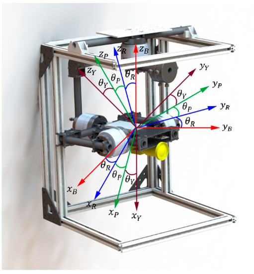
Figure 1.
Configuration of a three-axis stabilized platform.
2.2. Frictional Model
To accurately describe the dynamic response of the inertially stabilized platform, the Stribeck model is used to describe the dynamic friction and static friction functions of the three-axis stabilized platform [26]. According to the Stribeck model, with an increase in motion speed, the friction will decrease.
When , the static friction is presented by:
While, when , the dynamic friction is presented by:
where is driving force, is coulomb friction moment, is the maximum of the static friction, is the relative angular velocity between contact surfaces, is the scaling factors of viscous friction forces, are two exceedingly small positive constants.
2.3. Dynamics
According to the Euler equation, the dynamics of the three-axis stabilized platform can be modelled as follows:
where is the angular acceleration, is the angular velocity, is the force moment of the acting force, is each frame’s inertia moment.
Each frame of the three-axis stabilized platform is designed as axisymmetric. Therefore, the inertia product of each axis can be approximated to zero. The influence of the inertia product to the system can be ignored. Hence, each frame’s momentum of inertia can be approximated to a diagonal matrix as follows:
Imitating the processing of linearizing equilibrium points [27], quadratic terms can be ignored. Then, the dynamics can be modeled:
where are the torques of the motor acting on the frame, are unknown disturbances including the friction.
2.4. State Space Equation
Transforming (5)–(7) into matrix equation, it yields:
where:
Simplifying (8) as follows, we have:
where , , , , , , .
Transforming (9) into the system state space equation, it yields:
where is the friction between contact surfaces, is the sum of unknown external disturbances of the system, the matrix . The state variables are and , respectively, where are the angles of the platform and wgx, wgy, wgz are angular velocities of the platform.
3. Controller Design
3.1. Global Fast Sliding Mode Controller
Classical fast terminal sliding surface is obtained as follows:
where is the state vector of the system, are the positive parameters of the sliding surface, and are odd numbers.
Transforming (11), it yields:
Computing the integral of (12), it yields:
From (13), the time from the current state to equilibrium state can be obtained as follows:
Because the classical fast terminal sliding mode introduces the nonlinear parameter , which is effectively improves the convergence speed of the changing from controlled vector to the equilibrium state x = 0. The farther the distance from the controlled vector to the equilibrium state is, the faster the convergence speed of the controlled carriable is. However, the convergence speed of the classical fast terminal controller is not always the fastest. The linear sliding mode control is faster than the classical fast terminal sliding mode control as the controlled state vector gradually converges to zero. Two different kinds of sliding mode combine to global fast terminal sliding mode control. The global fast terminal sliding surface is obtained as follows:
where is the stated vector of the system, are the parameter of the surface. are positive odd numbers.
Similarly, the time from current state to equilibrium state is obtained as follows:
As the controlled state vector is far away from the equilibrium state, the convergence speed of the system depends on . When is near to the equilibrium state, the convergence speed of the system depends on , decreased exponentially. In that case, global fast terminal sliding mode control can preserve the equilibrium-state-approached the speed in linear sliding mode. Since the terminal attractor is chosen, the controlled state vector converges in a finite time. Therefore, the controlled state vector can make converging to the equilibrium state faster and more accurate.
Considering the modeling uncertainty and the nonlinear friction between the contact surfaces of the three-axis stabilized platform, Equation (10) is the system state space. Assume the desired attitude of the three-axis platform is . are the desired angel. The tracking angle error is defined as:
where is the angle relative to inertial space of the three-axis platform, is the differential of which is the angular velocity relative to inertial space of the three-axis platform, is the tracking angle error.
The global fast terminal sliding surface (15) is defined as follows:
where , p and q are positive odd numbers.
Differentiating (18), the following equation is obtained as:
The global fast terminal sliding mode controller is designed as:
where and are positive odd numbers.
Substituting (20) into (21) is obtained as follows:
where .
By solving (21), the time from current state to equilibrium state is obtained as follows:
As ,
Above all, the tracking angle error converge along to the neighborhood of sliding surface in finite time is obtained as follows:
Radius of convergence is obtained as follows:
3.2. Non-Linear Differentiator
The design of the close-loop controller based on NNFTSMC is shown in Figure 2. In the global fast sliding mode controller, the desired attitude of the three-axis stabilized platform is inputted to the controller. It is necessary to obtain the differential of the desired signal and the differential of the differential signal in the controller. In the PID controller, the differential method is commonly used to find the differential value of the error. The differential method can achieve good tracking when there is no signal noise. However, when there is noise in the signal, the noise will amplify together with the signal. Therefore, the signal will be distorted. Han [28] proposed a tracker that has good tracking effect to deriving noisy signals to calculate the differential of input signal.
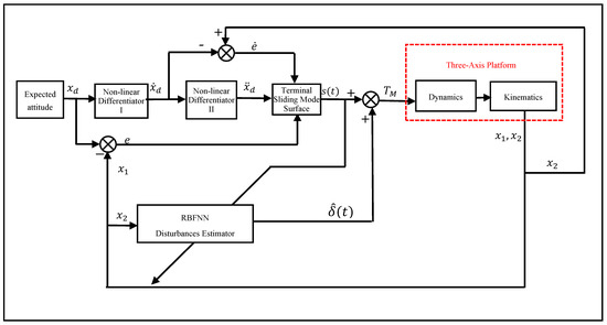
Figure 2.
Diagram of the close-loop controller based on NNFTSMC.
In our proposed control system, two non-linear differentiators are designed to calculate the desired angular velocity and the desired angular acceleration relative to inertial space of the three-axis platform.
The first non-linear differentiator is obtained as follows:
The second non-linear differentiator is obtained as follows:
where is the desired angle relative to inertial space of the three-axis platform, is the desired angular velocity relative to inertial space of the three-axis platform, is the input to the non-linear differentiator II and the desired angle relative to inertial space of the three-axis platform, is the desired angular velocity relative to inertial space of the three-axis platform, is the break between two signal acquisitions, is the level of the tracking speed of nonlinear tracking differentiator.
is the optimal control synthesis function as follows:
where:
In (28) and (29), .
3.3. RBF Neural Network Based Friction Estimator
The control law of the global fast sliding mode is continuous so that the chattering behaviors can be eliminated. However, the anti-interference performance of the controller is poor. The friction in (19) has a non-linear relationship with angular velocity. The friction between the contact surfaces will reduce the dynamic performance of the system. Therefore, estimating and compensating the friction is an important issue in optimizing the system performance. The RBF neural network has excellent performance of the nonlinear approximation and the environment adaptation. The dynamic performance of the global fast terminal sliding mode controller can be improved by using RBF neural networks as the perturbation estimator.
Many parameters such as the uncertain nonlinear function in the dynamic system are difficult to measure accurately. The existence of external disturbances makes it difficult to get a precise mathematical model. In this paper, RBF neural network is utilized to emulate the uncertain nonlinear function by creating an adaptive control law. Figure 3 shows a MIMO RBF neural network structure, which consists of three-layered network structures, i.e., the input layer, hidden layer and output layer. By the simulation of the results, the more neurons employed, the heavier calculation burden is, the less neurons employed, the less precision the results are. In consideration of the hardware capabilities and the suited accuracy, seven neurons are the best choice. So, there are seven neurons employed in the hidden layer of this paper.
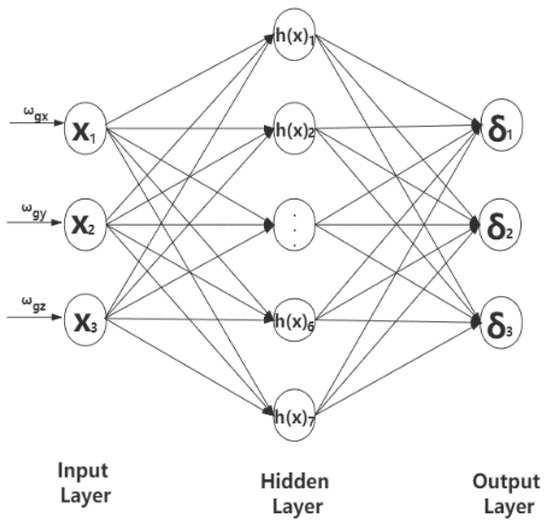
Figure 3.
MIMO RBF neural network structure.
RBF network is a kind of local approximation network with Gaussian function. Compared with BP network, RBF network can obtain faster learning speed to avoid falling into local optimum, and it is easier to meet the real-time requirement.
In the case of the mathematical model with uncertainty, the sliding mode control law is obtained as follows:
where , is the network input; is the network ideal weight; is the network Gaussian basis function output; is the network approximation of error; is centroid coordinates and propagation range of the neuron basis function in the hidden layer of the network.
Input the angular velocity into the RBF neural network, the output of the neural network is as follows:
If , the error of the estimator is .
The updated law of the RBF neural network is obtained as:
where is a positive definition matrix.
By adding the neural network perturbation estimator to (20), the result is presented as follows:
4. Stability Analysis
The network weights can be updated by (33). Combined with (34), the network weights can guarantee the stability of the closed-loop system. The dynamic error of the system can converge to zero.
Proof.
Global fast sliding mode controller includes control laws and the neural network estimator compensation law, let the Lyapunov function candidate be defined as follows:
where is a parameter of the controller, is a positive-definite matrix, and is the trace operator.
The derivative of Lyapunov function along to time as follows:
Substituting (34) into (36) is obtained as follows:
Substituting (33) into (37), we yield:
where is a positive definite matrix, .
As is a positive definite matrix, can be expressed as follows:
Just make sure is even, and then .
Therefore, according to Lyapunov stability theorem, the closed-loop system is stable, which means the sliding surface is stable. □
5. Simulation Results
In order to illustrate the effectiveness of the proposed control scheme, two simulations for trajectory tracking of the three-axis platform are performed in MATLAB environment. Physical parameters of the three-axis platform are listed in Table 1. In addition, the performance of the NNFTMC control method is compared with the SMC control method, the fast terminal sliding mode control (FTSMC) method and conventional PID control method considering the uncertainties and external disturbances of the model in the simulations. The physical parameters of the three-axis stabilized platform are listed in Table 1. The neural networks include seven neurons and the parameters of the control scheme that are proposed in this paper are selected as:

Table 1.
Physical parameters of the three-axis stabilized platform.
5.1. Non-Linear Differentiator
In the simulation environment, the input signal is designed with a sampling frequency of 500 Hz. The tracking speed r of the two-stage nonlinear tracking differentiator is 40 and 100 for each of the two stages. In the noise-free environment, the differential method and the non-linear tracking differentiator are used to obtain the differential of the signal, respectively. The results are shown in Figure 4, where is desired signal of angular velocity, is the signal by using the nonlinear tracking differentiator, is the signal by using the difference method.
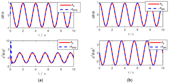
Figure 4.
Trajectory (noise-free) tracking results by using different method. (a) Trajectory tracking by using nonlinear tracking differentiator. (b) Trajectory tracking by using the difference method.
The tracking effect of the difference method is better than the nonlinear tracking differentiator in an ideal input signal. However, in practical applications, the noise of the input signal is unavoidable. The structure of the difference method itself will amplify the noise, and the noise signal is added to the simulation environment as a random signal with an amplitude of 0.01. The differential method and the nonlinear tracking differentiator are used again to obtain the differentiation of the signal, respectively, and the results are shown in Figure 5.
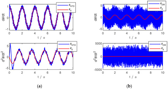
Figure 5.
Trajectory (with noise) tracking results by using different method. (a) Trajectory tracking by using nonlinear tracking differentiator. (b) Trajectory tracking by using the difference method.
As can be seen in Figure 5, the input signal is mixed with noise, the differential method used to obtain the differential of the signal has been completely incorrect and may even cause the controller to fail; the differential of the signal obtained using a nonlinear tracking differential still has some tracking capability.
5.2. Simulation of Sine Trajectory Tracking
The equation of the sine trajectory is given as:
where is the expected trajectory, are external disturbances.
The system sampling frequency is set as 1 kHz, and the runtime is set as 5 s. The angular velocity with external disturbance and the attitude angle of the platform in the simulation of attitude locking tracking trajectory are shown in Figure 6 and Figure 7, respectively.
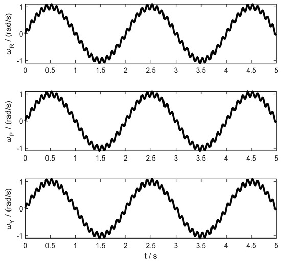
Figure 6.
The angular velocity with external disturbance of the platform in the simulation of sine trajectory.
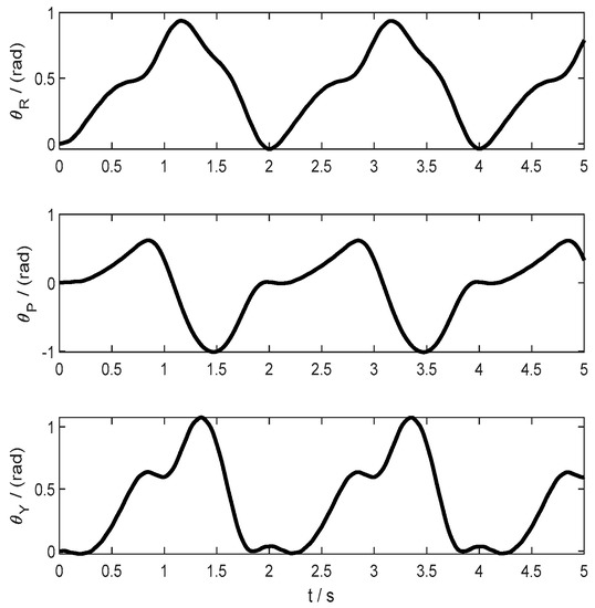
Figure 7.
The angle of the platform in the simulation of sine trajectory.
The sine trajectory tracking error of the simulation with traditional PID controller, SMC controller, FTSMC controller and NNFTSMC controller is presented in Figure 8. Figure 9 presents the attitude tracking result of the platform. In Figure 10 the angular velocities of the platform in three axes are shown. Figure 8, Figure 9 and Figure 10, present that compared with PID and SMC, NNFTSMC has faster response in servo control. The three-axis stabilized platform can maintain the desired attitude relatively well by using NNFTSMC control law. Compare with FTSMC, the addition of the prediction of friction by neural networks makes the NNFTSMC getting better tracking capability.
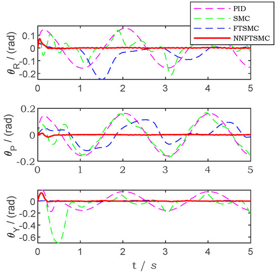
Figure 8.
The trajectory tracking error by using different controllers in the simulation of sine trajectory.
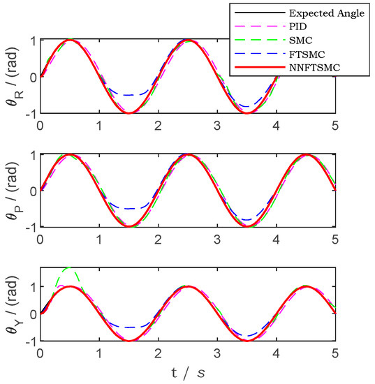
Figure 9.
The attitude of the platform by using different controllers in the simulation of sine trajectory.
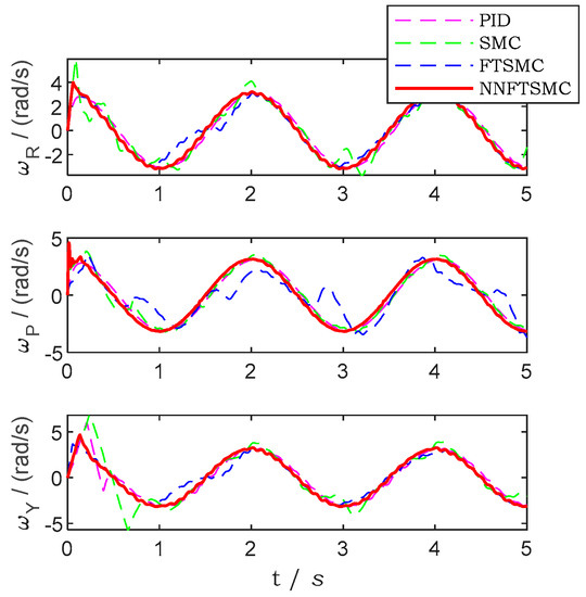
Figure 10.
The angular velocity of the platform by using different controllers in the simulation of sine trajectory.
Integral absolute error (IAE) and integrated square error (ISE) are important performance metrics to analyze the result of the control system.
where is the deviation of actual output from desired output, is the time.
The IAE and ISE results of the simulation of sine trajectory are shown in Table 2 and Table 3, respectively. It is observed from Table 2 and Table 3 that the proposed control scheme has a smaller steady-state error. The steady-state error gradually converges to zero.
Table 2.
The comparison of sine trajectory tracking results of IAE.
Table 3.
The comparison of sine trajectory tracking results of ISE.
Since PID control method is an error-based control strategy, there is a phase lag in the control pose therefore this method cannot control the attitude immediately. Although the NNFTSMC controller is designed without a switching term, the parameter is a variable parameter. The parameter is still considered as the switching term of the system in the sense of the output, which leads to the chatter of the system output. However, the dynamic error and steady-state error are smaller compared to SMC.
5.3. Simulation of Attitude Locking
The desired attitude and external disturbances of three axes are given as:
The system sampling frequency is set to 1 kHz, the runtime is set to 5 s. The angular velocity with external disturbance and the attitude angle of the platform in the simulation of attitude locking tracking trajectory are shown in Figure 11 and Figure 12, respectively.
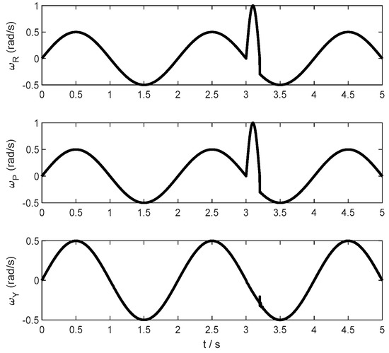
Figure 11.
The angular velocity with external disturbance of the platform in the simulation of attitude locking tracking trajectory.
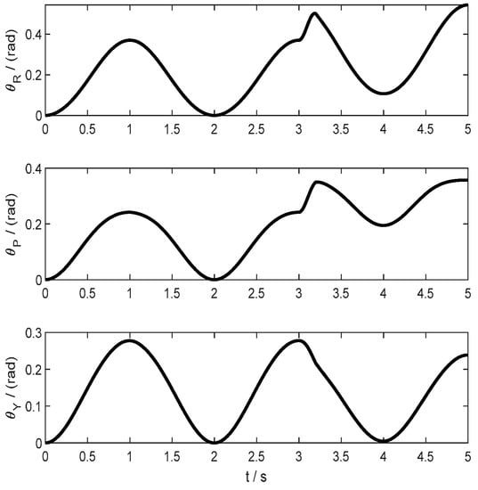
Figure 12.
The angle of the platform in the simulation of attitude locking tracking trajectory.
The attitude locking tracking trajectory error of the simulation with traditional PID controller, SMC controller, FTSMC controller and NNFTSMC controller is presented in Figure 13. Figure 14 presents the attitude tracking result of the platform. In Figure 15 the angular velocities of the platform in three axes are shown. Figure 13, Figure 14 and Figure 15 present that the NNFTSMC control law has good anti-interference performance compared to PID, SMC and FTSMC. By using neural networks to add the prediction of friction, NNFTSMC has better stability than FTSMC. The three-axis stabilized platform can maintain the desired attitude relatively well by using NNFTSMC control law. The IAE and ISE results of the simulation of attitude locking are shown in Table 4 and Table 5, respectively. Through the simulation of attitude locking, the NNFTSMC control law has better robustness, less steady-state and dynamic errors than the PID, SMC and FTSMC. Meanwhile, the NNFTSMC has better response speed in servo control for nonlinear systems with uncertainty of system parameters.
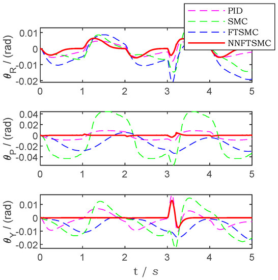
Figure 13.
The trajectory tracking error by using different controllers in the simulation of attitude locking.
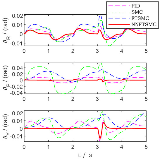
Figure 14.
The attitude of the platform by using different controllers in the simulation of attitude locking.
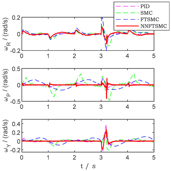
Figure 15.
The angular velocity of the platform by using different controllers in the simulation of attitude locking.
Table 4.
The comparison of the simulation of attitude locking tracking results of IAE.
Table 5.
The comparison of the simulation of attitude locking tracking results of ISE.
6. Conclusions
This paper designs the NNFTSMC based controller for the three-axis stabilized platform, which combines the global fast terminal sliding mode control method with the neural network technique. The chatter effect of the system output in sliding mode control algorithm can be eliminated by designing the sliding mode surface without the switching term and the saturation function. The global fast terminal sliding mode controller can make the controlled state vector approach the sliding mode surface in a finite time. Meanwhile, the RBF neural network is employed as a disturbance estimator to compensate for the nonlinear friction of the contact surface. In comparison with the FTSMC, the addition of RBF neural network gives NNFTSMC better stability and tracking capability. According to the Lyapunov theory, the stability of the proposed NNFTSMC method is proved. A nonlinear differentiator is used instead of the difference method to differentiate the signal. The experimental results show that the nonlinear differentiator has better robustness for the noisy input signal. In order to illustrate the effectiveness of the proposed control scheme, the simulation of Sine Trajectory and attitude locking are presented. The simulation results show that the NNFTSMC controller responds faster under the same system perturbation. The tracking error can gradually converge to zero in the servo control.
Author Contributions
W.F. and X.Z. proposed the algorithm and wrote the paper, as well as analyzed the data. Both authors have read and agreed to the published version of the manuscript.
Funding
This work is supported by the National Natural Science Foundation of China (No. 61703012, 51975011) and the Beijing Natural Science Foundation (No. 4182010).
Data Availability Statement
The data that support the findings of this study are available from the corresponding author upon reasonable request.
Conflicts of Interest
The authors declare no conflict of interest.
References
- Wang, Y.; Tian, D.; Dai, M. Composite hierarchical anti-disturbance control with multisensor fusion for compact optoelectronic platforms. Sensors 2018, 18, 3190. [Google Scholar] [CrossRef] [Green Version]
- Zhou, X.; Yang, C.; Zhao, B.; Zhao, L.; Zhu, Z. A high-precision control scheme based on active disturbance rejection control for a three-axis inertially stabilized platform for aerial remote sensing applications. J. Sens. 2018, 2018, 7295852. [Google Scholar] [CrossRef]
- Zhong, M.Y.; Jiao, C.B.; Li, S.S.; Zhao, Y. Study on the compensation method for disturbance torque of three-axis inertially stabilized platform based on PMI. Chin. J. Sci. Instrum. 2014, 35, 781–787. [Google Scholar]
- Paik, S.; Nandakumar, M.P.; Ashok, S. Model development and adaptive control implementation of a 3-axis platform stabilization system. In Proceedings of the 2015 International Conference on Smart Technologies and Management for Computing, Communication, Controls, Energy and Materials (ICSTM), Chennai, India, 6–8 May 2015; pp. 526–531. [Google Scholar]
- Li, S.; Zhong, M.; Qin, J. The internal model control design of three-axis inertially stabilized platform for airborne remote sensing. In Proceedings of the 2012 8th IEEE International Symposium on Instrumentation and Control Technology (ISICT), London, UK, 11–13 July 2012; pp. 5–10. [Google Scholar]
- Fang, J.; Yin, R.; Lei, X. An adaptive decoupling control for three-axis gyro stabilized platform based on neural networks. Mechatronics 2015, 27, 38–46. [Google Scholar] [CrossRef]
- Zhou, X.; Zhao, B.; Liu, W.; Yue, H.; Yu, R.; Zhao, Y. A compound scheme on parameters identification and adaptive compensation of nonlinear friction disturbance for the aerial inertially stabilized platform. ISA Trans. 2017, 67, 293–305. [Google Scholar] [CrossRef] [PubMed]
- Han, J. From PID to active disturbance rejection control. IEEE Trans. Ind. Electron. 2009, 56, 900–906. [Google Scholar] [CrossRef]
- Mao, J.; Li, S.; Li, Q.; Yang, J. Design and implementation of continuous finite-time sliding mode control for 2-DOF inertially stabilized platform subject to multiple disturbances. ISA Trans. 2019, 84, 214–224. [Google Scholar] [CrossRef] [PubMed]
- Zhou, X.; Jia, Y.; Zhao, Q.; Cai, T. Dual-rate-loop control based on disturbance observer of angular acceleration for a three-axis aerial inertially stabilized platform. ISA Trans. 2016, 63, 288–298. [Google Scholar] [CrossRef]
- Zhang, W.; Ping, J. Research of sliding mode variable structure control of PMSM based on composite reaching law. In Proceedings of the 2012 3rd International Conference on Mechanic Automation and Control Engineering, Baotou, China, 27–29 July 2012; pp. 1715–1718. [Google Scholar]
- Utkin, V.I.; Chang, H.C. Sliding mode control on electro-mechanical systems. Math. Probl. Eng. 2002, 8, 451–473. [Google Scholar] [CrossRef] [Green Version]
- Zhang, M.; Guan, Y.; Zhao, W. Adaptive super-twisting sliding mode control for stabilization platform of laser seeker based on extended state observer. Optik 2019, 199, 163337. [Google Scholar] [CrossRef]
- Sharifnia, M. Nonlinear dynamics of flexible links in planar parallel robots using a new beam element. J. Vib. Control 2020, 26, 475–489. [Google Scholar] [CrossRef]
- Boscariol, P.; Scalera, L.; Gasparetto, A. Nonlinear Control of Multibody Flexible Mechanisms: A Model-Free Approach. Appl. Sci. 2021, 11, 1082. [Google Scholar] [CrossRef]
- Zhang, Q.; Zhao, X.; Liu, L.; Dai, T. Adaptive sliding mode neural network control and flexible vibration suppression of a flexible spatial parallel robot. Electronics 2021, 10, 212. [Google Scholar] [CrossRef]
- Chan, J.C.L.; Lee, T.H. Sliding mode observer-based fault-tolerant secondary control of microgrids. Electronics 2020, 9, 1417. [Google Scholar] [CrossRef]
- Qiao, Z.; Shi, T.; Wang, Y.; Yan, Y.; Xia, C.; He, X. New sliding-mode observer for position sensorless control of permanent-magnet synchronous motor. IEEE Trans. Ind. Electron. 2012, 60, 710–719. [Google Scholar] [CrossRef]
- Lei, X.; Zou, Y.; Dong, F. A composite control method based on the adaptive RBFNN feedback control and the ESO for two-axis inertially stabilized platforms. ISA Trans. 2015, 59, 424–433. [Google Scholar] [CrossRef]
- Zhang, L.; Xia, Y.; Zhang, W.; Yang, W.; Xu, D. Adaptive command-filtered fuzzy nonsingular terminal sliding mode backstepping control for linear induction motor. Appl. Sci. 2020, 10, 7405. [Google Scholar] [CrossRef]
- Wang, J.; Lee, M.C.; Kim, J.H.; Kim, H.H. Fast fractional-order terminal sliding mode control for seven-axis robot manipulator. Appl. Sci. 2020, 10, 7757. [Google Scholar] [CrossRef]
- Li, Y.; Qiang, S.; Zhuang, X.; Kaynak, O. Robust and adaptive backstepping control for nonlinear systems using RBF neural networks. IEEE Trans. Neural Netw. 2004, 15, 693–701. [Google Scholar] [CrossRef]
- Yang, F.; Paindavoine, M. Implementation of an RBF neural network on embedded systems: Real-time face tracking and identity verification. IEEE Trans. Neural Netw. 2003, 14, 1162–1175. [Google Scholar] [CrossRef]
- Lu, X.; Zhang, X.; Zhang, G.; Fan, J.; Jia, S. Neural network adaptive sliding mode control for omnidirectional vehicle with uncertainties. ISA Trans. 2019, 86, 201–214. [Google Scholar] [CrossRef] [PubMed]
- Zhao, L.; Liu, X.Q.; Chen, C.; Bai, X.F. Rbf neural network of multi-motor system pid control based on neuron decoupling technology. Electr. Drive 2009, 39, 59–62. [Google Scholar]
- Kong, X.; Wang, Y.; Jiang, S. Friction chatter-compensation based on stribeck model. J. Mech. Eng. 2010, 46, 68–73. [Google Scholar] [CrossRef]
- Kennedy, P.J.; Kennedy, R.L. Direct versus indirect line of sight (LOS) stabilization. IEEE Trans. Control Syst. Technol. 2003, 11, 3–15. [Google Scholar] [CrossRef]
- Han, J.Q. From PID technique to active disturbances rejection control technique. Control Eng. China 2002, 9, 13–18. [Google Scholar]
Publisher’s Note: MDPI stays neutral with regard to jurisdictional claims in published maps and institutional affiliations. |
© 2021 by the authors. Licensee MDPI, Basel, Switzerland. This article is an open access article distributed under the terms and conditions of the Creative Commons Attribution (CC BY) license (https://creativecommons.org/licenses/by/4.0/).