Time-Varying Deterministic Volatility Model for Options on Wheat Futures ^†

Abstract

This study introduces a robust model that captures wheat futures’ volatility dynamics, influenced by seasonality, time to maturity, and storage dynamics, with minimal calibratable parameters. Our approach reduces error-proneness and enhances plausibility checks, offering a reliable alternative to models that are difficult to calibrate. Transferring estimated parameters from liquid to illiquid markets is feasible, which is challenging for models with numerous parameters. This is of practical importance as it improves the modeling of volatility in illiquid markets, where price discovery is less efficient. In liquid markets, on the other hand, where speculative activity is high, we find that implied volatility is usually the best measure. Additionally, the introduced volatility model is suitable for pricing options on wheat futures as a risk-neutral measure.

1. Introduction

Financialization in commodity markets has manifested in the growing participation of financial investors, such as hedge funds and index funds, which has led to a greater integration with broader financial markets and increased speculative trading activity. It is well known that this activity influences the price discovery of futures and options. Refs. [1,2] provide a comprehensive overview.

However, financialization does not only mean that speculators influence the price discovery process; it also means that market participants who are not directly involved in price formation and have no direct interest in the physical product use the traded price information for derived contracts, such as crop failure insurance. The appropriate use of price information prerequisites a market with a well-functioning price discovery process. Ref. [3] discusses the mechanisms through which low liquidity can hinder the process of price discovery. Ref. [4] highlights that in commodity markets, tight funding conditions can lead to reduced market liquidity, hampering the overall market efficiency.

These conditions pose a significant challenge for market participants, such as insurers or farmers, who use the option price information to value derivative products or to estimate hedging costs. In illiquid markets, in particular, where options are rarely traded or not at all, option pricing models have to take on this task. This is usually associated with two challenges: firstly, a correct option pricing model, and secondly, an appropriate dataset for calibrating the models. The number of possible option pricing models for commodity futures is diverse but differs mainly in volatility modeling; see [5]. A bigger challenge is calibrating volatility when adequate data are unavailable, especially for illiquid markets or commodities without a dedicated marketplace.

Accurately pricing options on wheat futures is paramount for participants in agricultural markets, including traders, insurers, and policymakers. The unique characteristics of wheat futures, influenced by seasonality, time to maturity, and storage dynamics, present significant challenges for traditional option pricing models. The [6] model, a cornerstone in the field, assumes constant volatility, which fails to capture the systematic variations observed in wheat futures markets.

This study aimed to bridge the gap between traditional volatility models and more sophisticated models that capture all these characteristics but presume an adequate but mostly large dataset. We provide a robust model that captures the dynamics of wheat futures volatility, where we only need to calibrate a few parameters, and we can visually plausibilize the volatility pattern, ensuring that the estimated volatility pattern corresponds to the harvest cycle. We incorporate seasonal patterns, the time-to-maturity effect, and storage dynamics through the U.S. stocks-to-use ratio.

More sophisticated models with a high number of estimated parameters are error-prone; they make plausibility checks almost impossible, which increases the risk of using unspecified models. An economic interpretation of the parameters in these models is also extremely challenging, especially if a market-specific roll-over strategy for futures contracts is used to create the time series, as this influences the mean reversion parameters and the average time-to-maturity effect, for example. This is a significant disadvantage of these models, and we want to overcome this with our robust model.

We focus on options that cover a marketing year from September to August of the following year. As the option is written from the future, we model the futures price as the underlying price and not a continuous spot price.The price of a future’s contract represents the price of wheat delivered at a specific location at the time of the futures’ expiration. Any price expectations, such as seasonal price variability, are already reflected in futures prices and thus do not need to be considered when valuing options. (More formally, a futures contract, as the option’s underlying, is itself tradeable and requires no capital. Thus, the futures’ price must have a zero drift under the risk-neutral measure in order to avoid any arbitrage opportunities. It follows that all available information is incorporated in the future’s price, which itself determines the option’s price.) This substantially reduces the number of model parameters and, in addition to that, the risk of over-parametrization.

The stocks-to-use ratio is unsuitable for predicting volatility, mainly if shortages rarely occur during the calibration period, but it can be helpful for risk modeling. In liquid markets, where speculative activity is high, implied volatility is generally considered the best measure. However, our model offers a practical solution in less liquid markets.

With some limitations, we can transfer the estimated parameters from liquid markets to similar illiquid markets, which is difficult for more sophisticated models requiring a large number of parameters. This application has significant implications, such as crop failure insurance, and has practical relevance for market participants, providing a more effective tool for modeling volatility in illiquid markets. The introduced volatility model is suitable for pricing European options on wheat futures in a risk-neutral measure.

2. Literature Review

The price of a future’s contract represents the price of wheat delivered at a specific location at the time of the futures’ expiration. Any price expectations, such as seasonal price variability, are already reflected in future prices and thus do not need to be considered when valuing options.

Many studies have documented that the volatility of a future’s contract is time-varying and has at least two deterministic components. The first refers to the “Samuelson effect” [7], which posits that a future’s price volatility increases as the contract approaches expiration. The second component refers to the observed seasonal pattern of a contract’s price volatility over a year. Ref. [8] provides a theoretical foundation for this effect, linking it to the flow of market-relevant information that intensifies as the delivery date nears. This effect is particularly relevant for agricultural commodities, where uncertainties about final yields and market conditions peak during harvest.

Seasonality in commodity prices, particularly agricultural products, has been extensively documented. Ref. [9] highlighted the influence of harvesting cycles on commodity prices, leading to predictable patterns in volatility. Also, ref. [10] showed that for the three main crops analyzed, i.e., wheat, the seasonal pattern is strongly related to the crop cycle. Ref. [11] analyzed the characteristics of soybean futures and options based on a spot price process. They found price mean reversion to a seasonally varying mean and seasonal variation in the volatility. Ref. [12] extended the two-factor model [13] by adding a deterministic seasonal component and applying it to corn, soybean, and wheat futures. Ref. [14] used a multi-factor model to model the volatility of future prices in agricultural markets. The time series are created based on a pre-defined roll-over strategy. The price time series constructed in this way contains several expiry months. The seasonal component is incorporated into the stochastic volatility dynamics, and they account for the Samuelson effect with a maturity-dependent damping term. A total of 19 parameters are calibrated for the model.

Storage is crucial in buffering supply and demand shocks, affecting commodity price volatility. Refs. [15,16,17]’s theoretical models emphasize the stabilizing effect of storage. Low inventory levels, often proxied by the stocks-to-use ratio, lead to higher volatility, especially during critical periods such as harvest time.

Empirical research has shown that storage levels significantly impact price volatility. Refs. [18,19] included storage dynamics in their models, finding that lower inventory levels are associated with higher volatility. This relationship underscores the importance of incorporating storage effects into volatility models for better predictive accuracy.

Integrated Volatility Models

Ref. [20] estimated a spot price model for soybeans, acknowledging that commodities exhibit seasonal effects in the spot price level and volatility. Ref. [21] fitted market option prices on wheat futures. They included the seasonal and maturity effects of the volatility specification to the jump diffusion option pricing model from [22]. Ref. [18] focused on the soybean spot price process and included a deterministic component to describe time-varying volatility. Ref. [19] extended a one- and a two-factor spot price model by allowing for seasonal changes in the volatility during a calendar year and applied the models to corn, soybean, heating oil, and natural gas options. Ref. [23] proposed a seasonally varying long-run mean-variance process and applied its seasonal stochastic volatility model to natural gas and corn futures options.

The main commonality of these models is that options are valued on spot prices with seasonal characteristics. However, seasonality in the spot price process is already reflected in future prices and, therefore, does not need to be considered (see [5], p. 411). Another disadvantage is the time-to-maturity effect of futures, which is not reflected in the spot price process and, therefore, is ignored in many applications.

When modeling an option directly on a futures price, one substantially reduces the number of model parameters. The model in [24] needs a total of eight parameters (three volatilities, three correlations, and two speeds of mean reversion parameters), which have to be calibrated on a reliable database for calculating European option prices on commodity futures. Ref. [19] used up to six parameters calibrated on the cross-section of implied volatilities, i.e., options on future contracts with different expiration dates. However, as shown in [11], each contract maturity has its seasonal pattern, and thus, calibrating parameters across maturities lead to distorted parameter values.

Several recent studies have explicitly focused on modeling the futures price as the underlying asset. For instance, using a Bayesian time-varying coefficient approach, ref. [25] examined the dynamics between trading volume, volatility, and open interest in agricultural futures markets. Ref. [13] developed another difficult-to-calibrate model for the valuation of options on commodity futures, in which the price behavior of futures is derived from spot prices in combination with stochastic term structures of convenience yields and interest rates.

The remainder of this paper is structured as follows. Section 3 describes the data used in the empirical analysis. Section 4 describes the volatility model and the assessment of the impact of inventories. Information is provided on the statistical methods, used and the out-of-sample test is described. Section 5 contains the main empirical results of this study. We analyze the out-of-sample predictive ability and the stability of the parameters. Additionally, we interpret the parameters found and how they can be plausibilized. In Section 6, we demonstrate that the volatility model can be integrated into the option pricing model of Black (1976). Finally, we conclude the paper in Section 7.

3. Data Description

3.1. Wheat Futures

Seasonality and the time-to-maturity effect of volatility are analyzed for wheat future contracts traded on four different commodity exchanges. Currently, the international and national (U.S.) benchmark for pricing wheat is the Chicago Mercantile Exchange (CME). Two other exchanges trade wheat in the U.S. but are less liquid. The Kansas City Board of Trade (KCBT) and the Minneapolis Grain Exchange (MGEX) differ from the CME in terms of wheat classes for delivery and respective delivery locations. The European benchmark for pricing physical wheat is the Milling Wheat No. 2 future contract, traded at the pan-European exchange (EURONEXT) in Paris. However, the EURONEXT has a substantially lower degree of trading volume than the U.S. counterparts ([26]). Trading activity, in terms of open interest and volume, grows considerably faster in Paris compared to the U.S. markets (see [27]), although on a lower level.

Futures are held for one year from September until August of the following year, i.e., one marketing year. Paris contracts are denominated in EUR.

The daily log returns are calculated for September wheat contracts over the period September 2000 to April 2018. One exception is Paris, where no September contracts are available between 2008 and 2014, and the November contract is used instead. We compute daily log returns according to the following:

$$r_{F_{T,t}}=ln\left({\displaystyle \frac{F_{T,t}}{F_{T,t-1}}}\right),$$

(1)

where $F_{T,t}$ is the future’s closing price at time t with an expiration date T. The main variable of interest is the annualized daily volatility for a calendar month, which is determined as follows:

$${\sigma }_m=\sqrt{252}\sqrt{{\displaystyle \frac{1}{N-1}}\sum _t^N{\left(r_{F_{T,t}}-{\overline{r}}_{F_T}\right)}^2},$$

(2)

where $r_{F_{T,t}}$ denotes the daily log return, N is the number of business days in the observation month, and ${\overline{r}}_{F_T}$ is the average log return over N days, i.e., from $t-1$ to $t-N$, and the term $\sqrt{252}$ annualizes the volatility estimator.

3.2. Wheat Option Contracts and Implied Volatility

Wheat options analyzed in this study are written on a pre-defined future’s contract. Only this future’s contract is deliverable when the option is exercised, not physical wheat, shipping documents, or related delivery notes. Since the option underlying itself is a tradeable contract, the option model simplifies to the standard option pricing model in [6], which was the first to provide a formula to value commodity options in terms of the future’s price.

Two aspects are important: first, the option’s maturity is typically shorter than the maturity of the underlying futures contract. For example, all U.S. option contracts expire on the last Friday of the month prior to the futures expiration month, which is roughly half a month (see CME exchange rulebook, chapter 14A, and MGEX Rulebook chapter 14, option specifications hard red spring wheat). The time spread at the EURONEXT is slightly higher, i.e., the contract’s expiry is normally the 15th day of the month preceding the delivery month of the future’s contract, which is roughly 3 to 4 weeks (see EURONEXT, Technical specifications of the No. 2 Milling Wheat option contract, no. 10.2 Settlement procedure). Second, all options are American-style, i.e., the option may be exercised at any time up to its date of expiration. For further details, refer to the respective exchange rule books of the CME, the KCBOT, the MGEX, and the EURONEXT.

We take implied volatilities from at-the-money September wheat options, to avoid necessary moneyness approximations as suggested in [28]. The option’s underlying is a wheat future’s contract, which expires in September of the following year. Respective daily implied volatility data are taken from Bloomberg, where the reference model of [6] is used to compute the implied volatility from traded option prices).

3.3. Storage Data

The United States Department of Agriculture (USDA) is one of the most important information providers regarding U.S. and worldwide supply and demand estimates, crop conditions, planted acreage, stocks, and other fundamental information; see [29] or [30]. These data are published in a monthly World Agricultural Supply and Demand Estimates (WASDE) report.

The report provides the estimated ending stocks for wheat based on specific crop supply and demand forecasts. Forecasts, derived during a specific month, are published by the middle of the next month. The expected carry-over projection, which is a point prediction to the end of the current marketing year, is updated each month until the end of April and switches afterward into the projection of the following marketing year, where the old ending stocks become the new beginning stocks (ref. [31] provides a comprehensive explanation). This accounting procedure is taken into consideration when monthly times series of inventory data are constructed. In particular, the marketing year has been changed in accordance with the analyzed September wheat futures, i.e., ending projections are postponed until August. Ending stock predictions exclude seasonal components in the time series, which simplifies their application.

Inventory data generally grow with production and demand and are, therefore, usually normalized with consumption. The resulting ratio indicates the level of carry-over stock as a percentage of the total use and is known as the stocks-to-use ratio. For example, a 20% stocks-to-use ratio for wheat indicates that there is a 2.4 months supply of wheat in reserve; see [32]. In the following analysis, the stocks-to-use data is taken from the USDA WSDE report from the category U.S. Wheat Supply and Use, which summarizes all classes of wheat produced and primarily used in the United States.

4. Methodology for Volatility Analysis

4.1. Time to Maturity and Seasonality

A two-step procedure is used to decompose the volatility time series into (i) the volatility level, i.e., the center of gravity for a future’s volatility regarding the respective marketing year, and (ii) a seasonal plus time-to-maturity component ($\phi \left(t\right)$) describing the deterministic behavior of the volatility around the future’s volatility level. Intuitively, the volatility level corresponds to the volatility, which would be observed without seasonality in the contract’s price volatility. Following [18], the volatility ${\sigma }_{F,t}$ of a future F at time t has two components:

$${\sigma }_{F,t}={\overline{\sigma }}_F{e}^{\phi \left(t\right)},$$

(3)

where ${\overline{\sigma }}_F$ is the future’s volatility level, and $e^{\phi \left(t\right)}$ describes the seasonal behavior around the future’s volatility level at time t. Taking logs on Equation (3) yields the volatility decomposition:

$$ln\left({\sigma }_{F,t}\right)=ln\left({\overline{\sigma }}_F\right)+\phi \left(t\right).$$

(4)

Further, two seasonal functions are specified:

$${\phi }_t^S=\theta \sin \left(2\pi (t+\zeta )\right),\mathrm{and}$$

(5)

$${\phi }_t^{ST}=c+\beta (T-t)+\theta \sin \left(2\pi (t+\zeta )\right),$$

(6)

where ${\phi }_t^S$ denotes a sinusoidal function, $\theta$ denotes the amplitude parameter, i.e., the peak deviation of the function from zero, and $\zeta$ the respective phase parameter, i.e., where the oscillation is zero at time t. Equation (5) corresponds to the version in [18] and is denoted with $Model-S$. (Note that ref. [18] additionally specified a mean reversion process in the futures’ volatility. However, we skip the mean reversion component, since calibrated mean-reverting parameters are less reliable using a future’s life time with only 12 volatility observations per marketing year.)

Equation (6) additionally contains the time-to-maturity effect, denoted with $Model-ST$, where the constant c and $\beta (T-t)$ capture the impact of a decreasing time to maturity, and $(T-t)$ reflects the time to expiration in months.

4.1.1. Volatility Level Calibration

The volatility level is not observable and, therefore, must be estimated from historical volatility observations. This can be achieved by smoothing the time series of empirical volatility observations, while ensuring that seasonal effects are eliminated.

The trend decomposition is performed by smoothing the log volatility time series. Log volatility is used in order to assure that volatility must not be negative. This is ensured using an exponential function in the option pricing formula for the deterministic component in the volatility process. The smoothing is conducted using the robust version of ’Lowess’, which assigns lower weight to outliers in the regression (The used method assigns zero weight to data outside six mean absolute deviations; see [33]. The span is set according to the following rule of thumb: $span=12/(N/2)$, which is roughly 0.16).

4.1.2. Parameter Calibration

In the second step, the seasonality and time-to-maturity parameters ($\Phi$) have to be estimated. $Model-S$ requires the estimation of $\Phi \equiv \theta ,\zeta$, and for $Model-ST$, the parameters $\Phi \equiv c,\beta ,\theta ,\zeta$ have to be estimated to additionally take the time-to-maturity effect into account.

The set of parameters $\Phi$ are estimated by minimizing the root mean squared errors ($RMSE$) of the following objective function:

$$\begin{array}{cc}\hfill {\Phi }_t^{*}& =\underset{{\Phi }_t}{\arg \min }\mathrm{RMSE}\left({\Phi }_t\right)\hfill \\ \hfill & =\underset{{\Phi }_t}{\arg \min }\sqrt{{\displaystyle \frac{1}{N}}\sum _{t=1}^N{\left[ln\left({\sigma }_{F,T,t}\right)-\left(ln\left({\overline{\sigma }}_{F,T}\right)+{\widehat{\phi }}_t\left({\Phi }_t\right)\right)\right]}^2}\hfill \end{array}$$

(7)

where N refers to the number of observations, and T stands for the contract’s maturity. Further, imposing $\theta \ge 0$ and $\zeta \in [-0.5;0.5]$ ensures the parameters’ uniqueness.

4.2. Impact of Storage

The stocks-to-use ratio is an indicator of susceptibility to price peaks. According to [32], a stocks-to-use ratio for wheat below 20% has typically led to strong price advances. Ref. [34] used a more advanced model to calibrate critical values, but found similar levels slightly above 20%, while ref. [35] identified 18% on the global level.

Here, we focus on the question of whether there is a critical stocks-to-use level at which the parametrization of the seasonal component changes and to what extent. However, the statistical analysis is limited by the relatively small number of wheat shortages. Ref. [34], for example, found only five wheat stock-outs in a sample of 47 years and pointed to the trade-off between the available data and the statistical analysis:

“Large spikes are obviously quite rare in the available data. Even adding lesser spikes does not give us a sample useful for statistical analysis. Hence we must resort to a less formal analysis of the evidence.” [34], p. 50

Our data sample has similar characteristics: With a sample size of 212 months, only 15 months with a stocks-to-use ratio of less than 18% are observed. The number increases to 73 when the threshold is set to 26%.

Under these conditions, we searched for the critical stocks-to-use level using the following procedure: First, we calculate the RMSE for model $Model-ST$ according to Equation (7) over the entire sample period. In the second step, we split the data sample by setting the exogenous threshold for the stocks-to-use ratio ($stu$) between 18% and 26%. The RSME for the $S{T}_{stu}-model$ is then estimated as follows:

$$RMS{E}_{stu}=\sqrt{{\displaystyle \frac{1}{N}}\sum _{t=1}^{N}S{E}_{stu,t}},$$

(8)

with

$$S{E}_{stu}=\left\{\begin{array}{cc}{\left[ln\left({\sigma }_{F,T,t}\right)-\left(ln\left({\overline{\sigma }}_{F,T}\right)+{\widehat{\phi }}_t\left({\Phi }_{t,1}\right)\right)\right]}^2\hfill & \mathrm{if}st{u}_t<th,\hfill \\ {\left[ln\left({\sigma }_{F,T,t}\right)-\left(ln\left({\overline{\sigma }}_{F,T}\right)+{\widehat{\phi }}_t\left({\Phi }_{t,2}\right)\right)\right]}^2& \mathrm{if}st{u}_t\ge th,\end{array}\right.$$

where the threshold value $th$ is constrained to lie within the range $18\%\le stu\le 26\%$ of threshold variable $stu$. The $stu$ dependent set of parameters ${\Phi }_{t,1}$ (${\Phi }_{t,2}$) is estimated from each subsample, where the split of the sample is made below (above) the threshold value. Finally, we choose this $stu$ ratio as the critical value, corresponding to the lowest RMSE value. The smaller the RMSE of $Model-S{T}_{stu}$ compared to the RMSE of $Model-ST$, the greater the explanatory gain in the sample. However, this does not necessarily indicate good out-of-sample performance.

4.3. Model Comparison

The out-of-sample (OOS) model comparison in this study assumed that the risk assessment pertains to an entire marketing year, specifically focusing on the period from September to August. (For example, implied volatilities are often used for the valuation of crop insurance contracts. For wheat, such contracts are typically valued in autumn, i.e., before sowing, and expire after or around harvesting time.) Unlike traditional academic approaches emphasizing anticipated expected volatility, this study compared realized volatility with forecasted volatility over the specified period. This methodological divergence is crucial, as the accuracy of an option pricing model is typically assessed against the observed (traded) option price, as noted in [23,36].

The main focus of this analysis is to evaluate the predictive properties of the proposed deterministic volatility model by comparing the realized volatility with the model predictions and the volatility expected by the market, represented by implied volatilities from traded options. The latter is often regarded as the market’s best estimate of future volatility; see [5]. We, therefore, included it as a benchmark in our empirical comparative analysis. (Note that in the context of Black’s 76 model, volatility is defined as the square root of the average variance over the option’s remaining lifetime (Cox and Rubenstein, 1999). Implied volatility, on the other hand, reflects the market’s expectation of this integrated variance. For simplicity, this study disregards the market-price-of-risk process for F under the risk-neutral measure, which is typically embedded in the implied volatility.)

The following three volatility forecast models are used: (i) a 30-day rolling historical volatility (${\sigma }_{30d}$); (ii) volatility based on the $Model-ST$, i.e., seasonality model including the time to maturity, (${\sigma }_{ST}$); and (iii) a volatility based on the conditioned version of $Model-ST$ (${\sigma }_{S{T}_{stu}}$).

In the first step, the daily log returns ($r_{F_{T,t}}$) of wheat futures are calculated according to Equation (1), whereby the September contracts are held over a marketing year from the beginning of September to the end of August. The sample spans from 2000/09 to 2017/08 and includes 17 marketing years.

In a subsequent step, we utilize log returns over 30 days, commencing 30 business days prior to the observation date, to estimate rolling historical volatilities ${\sigma }_{30d}$. This estimation is performed using Equation (2). This rolling procedure yields, on average, 206 daily volatility forecasts per season.

To calculate daily volatility forecasts based on $Model-ST$ and its conditioned version, the following procedure is applied: first, calculate the volatility level $\overline{\sigma }$ using Equation (4) and set ${\sigma }_{30d}$ equal to ${\sigma }_{F,t}$, according to

$$ln\left(\overline{\sigma }\right)=ln\left({\sigma }_{30d,t}\right)-\phi \left(t\right).$$

(9)

Two functions describing the volatility’s seasonal and time-to-maturity behavior are specified, where the first ${\phi }_t^{ST}$ refers to $Model-ST$, and the second ${\phi }_{t,stu}^{ST}$ refers to $Model-S{T}_{stu}$ as the conditioned version. Hence, the volatility forecast is performed using the following equation:

$${\sigma }_{ST}=\overline{\sigma }\sqrt{{\displaystyle \frac{1}{T-t}}{\int }_t^T{e}^{2{\phi }_t^{ST}}dt}.$$

(10)

Replacing ${\phi }_t^{ST}$ with ${\phi }_{t,stu}^{ST}$ provides the conditioned volatility forecast ${\sigma }_{S{T}_{stu}}$.

Finally, realised volatility ${\sigma }_{real}$ is calculated on a daily basis according to

$${\sigma }_{real}=\sqrt{252}\sqrt{{\displaystyle \frac{1}{N}}\sum _t^N{\left(r_{F_{T,t}}-{\overline{r}}_{F_T}\right)}^2},$$

(11)

where N is the number of business days until the option’s expiration T, and ${\overline{r}}_{F_T}$ is the average log return over the remaining option’s lifetime, i.e., form t to T. Again, the term $\sqrt{252}$ annualizes the volatility. This procedure ensures that the same time horizon of realized, implied, and predicted volatility is used.

We use a rolling window of 13 years to calibrate the parameters based on monthly observations. The first calibration period is from September 2000 to August 2013, and the first out-of-sample month starts in September 2013. The out-of-sample period thus covers the period from September 2013 to July 2017. Note that we do not include the month of August as a forecast month in our out-of-sample test, as the options expire in this month.

Forecast Comparison

We compare the predictive performance of two volatility models using the pairwise [37] Diebold-Mariano (DM) test. The loss differential between two models is calculated as

$$d_t=e_{1,t+h}^2-e_{2,t+h}^2$$

(12)

where $e_{m,t+h}^2={\sigma }_{m,t+h}-{\sigma }_{real,t+h}$ refers to the forecast error at time t + h for model $m=1,2$.

The $DM$ statistic and the corresponding p-value allow us to determine whether there is a statistically significant difference in the predictive accuracy of the two models with the null hypothesis of equal predictive accuracy: $H_0:E\left[d_t\right]=0$ against the two-sided alternative, $H_1$. The two models do not have equal predictive accuracy $E\left[d_t\right]\ne 0$. The $DM$ statistic is

$$DM={\displaystyle \frac{\overline{d}}{\sqrt{{\widehat{\sigma }}_d^2}}}$$

(13)

where $\overline{d}={\displaystyle \frac{1}{T}}{\sum }_{t=1}^T{d}_t$ is the mean loss differential, and ${\widehat{\sigma }}_d^2$ is the variance of the loss differential, which can be estimated as

$$\widehat{{\sigma }_d^2}={\displaystyle \frac{1}{T}}\left({\gamma }_0+2\sum _{k=1}^{h-1}{\gamma }_k\right),$$

where ${\gamma }_k$ is the k-th autocovariance of the loss differential, which is given by

$${\gamma }_k={\displaystyle \frac{1}{T}}\sum _{t=k+1}^T(d_t-\overline{d})(d_{t-k}-\overline{d}).$$

The number of forecasts is denoted by T, and the forecast horizon, by h.

Under the null hypothesis of equal predictive accuracy, the DM test statistic follows an asymptotic standard normal distribution:

$$\mathrm{DM}\sim \mathcal{N}(0,1)$$

Ref. [38] addressed the potential size distortions in small samples and suggested correcting the variance of the DM statistic. They propose modifying the DM test by multiplying the DM statistic by a factor that accounts for the forecast horizon and the sample size. The adjusted DM statistic is given by

$$D{M}_{adj}=\sqrt{{\displaystyle \frac{T+1-2h+h(h-1)/T}{T}}}DM$$

(14)

where T is the number of out-of-sample observations, h is the mean forecast horizon, and $DM$ is the original Diebold–Mariano statistic.

5. Empirical Results

5.1. Seasonality and Time to Maturity

All parameters in Table 1 are estimated according to Equation (7) and are based on the logarithmic volatility. They can, therefore, be interpreted as percentage deviations from the logarithmic volatility level, which facilitates their interpretation.

Table 1. Seasonality and time-to-maturity effects.

	Panel A: Model–S		Panel B: Model–ST
Exchange	$\mathit{\theta }$	$\mathit{\zeta }$	$\mathit{\theta }$	$\mathit{\zeta }$	$\mathit{\beta }$	$\mathit{c}$
Chicago	0.21 ***	−0.21 ***	0.14 **	−0.22 **	−0.24 **	0.14 ***
Kansas	0.19 ***	−0.16 ***	0.14 ***	−0.15 ***	−0.15 ***	0.07 ***
Minneapolis	0.22 ***	−0.22 ***	0.17 ***	−0.22 ***	−0.18 *	0.11 ***
Paris	0.19 ***	−0.31 ***	0.13 ***	−0.38 ***	−0.27 ***	0.18 **

The table contains estimated sine parameters that describe the oscillation (seasonal pattern) in the volatility of September wheat future contracts. Panel A contains the estimation results of seasonal effects only, where the parameter $\theta$ represents the amplitude, i.e., the peak deviation in the function from zero, and $\zeta$ represents the phase, i.e., where the oscillation is zero at time t. Panel B contains, in addition, a constant parameter c, and the time-to-maturity effect is captured by $\beta$. Parameters are estimated using de-trended log volatility over the period September 2000 to April 2018, and the corresponding 10%/5%/1% levels of significance are marked with */**/***, respectively.

Panel A of Table 1 contains the results of the parameter estimation of $Model-S$ (Equation (5)), and Panel B, those of $Model-ST$ (Equation (6)). Starting with Panel A, the estimated amplitude parameters $\theta$ are very similar across markets, ranging from 0.19 for Kansas to 0.22 for Minneapolis, and are statistically significant at the 1% level. The phase parameters $\zeta$ indicate where the sine function begins in the marketing year. All estimated phase parameters are significant and lie between −0.16 for Kansas and −0.31 for Paris. This indicates that the sinusoidal function starts in autumn, with the lowest values in winter and the highest around summer.

The inclusion of the time-to-maturity effect $\beta$ reduces the amplitude parameters but leaves the phase virtually unaffected, as shown in Panel B of Table 1. These results are consistent with the findings in [39], i.e., a negative $\beta$ implies increasing volatility by shortening the time to expiration, suggesting that seasonal effects are overestimated if the “Samuelson effect” is ignored.

Parameter Interpretation

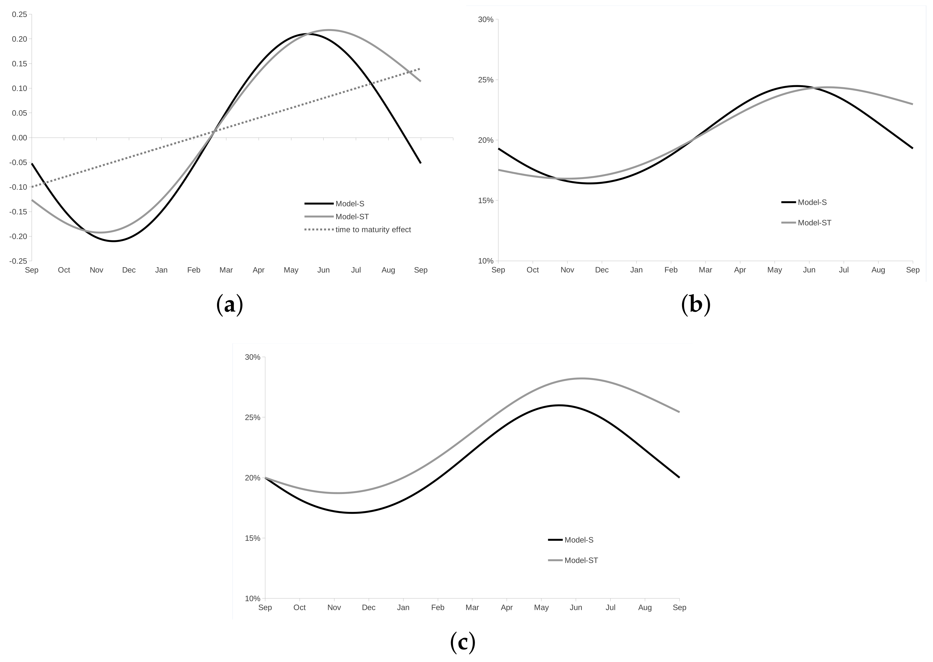
Figure 1a–c illustrate the effects of both $Model-S$ and $Model-ST$ on the deterministic volatility using the estimated parameters of Chicago wheat shown in Table 1.

Figure 1. Comparing deterministic volatility components between $Model-S$ and $Model-ST$. The figure shows the seasonal pattern of historical Chicago wheat future price volatility with September expiration. The volatility development spans the season from September to August, i.e., a marketing year. Seasonal parameters are taken from Table 1 with a calibration window between September 2000 and April 2018. (a) Development deterministic log volatility component; (b) development seasonal volatility with ${\overline{\sigma }}_F\left(T\right)=20\%$; (c) development seasonal volatility with ${\sigma }_F(t,T)=20\%$.

The development of deterministic log volatility components over the season from September to August is shown in Figure 1a. Consistent with other studies, both models show a similar pattern with the lowest volatility (ca. −20%) around December and the highest (ca. +20%) around harvest time in June and July. However, the impact differs when considering the time-to-maturity effect in $Model-ST$. The sinusoidal function in $Model-S$ forces the deterministic log volatility component toward zero in September and October, respectively. From July to September, in $Model-ST$, the seasonality is less pronounced as the time-to-maturity effect ensures that you do not have to go through the zero point as in $Model-S$, which allows for a higher log volatility component during the harvest period.

Figure 1b shows the development of deterministic volatility over a marketing year if the same average volatility of 20% is assumed. Although Figure 1a,b show similar patterns and amplitudes, there is a clear difference when the initial volatility is used instead of the future’s volatility level. Let us assume that a future’s volatility of 20% is estimated for the observation month of September. In this case, $Model-S$ implies a lower volatility level of 20.5% compared to $Model-ST$ with 22.9%. This is because the seasonal volatility reduction in September is less pronounced for $Model-S$ than for $Model-ST$. As a result, the volatility of $Model-ST$ is greater than that of $Model-S$ for all months of the marketing year, with significant differences of 27.5% and 23.6%, respectively, during the harvest period.

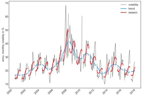
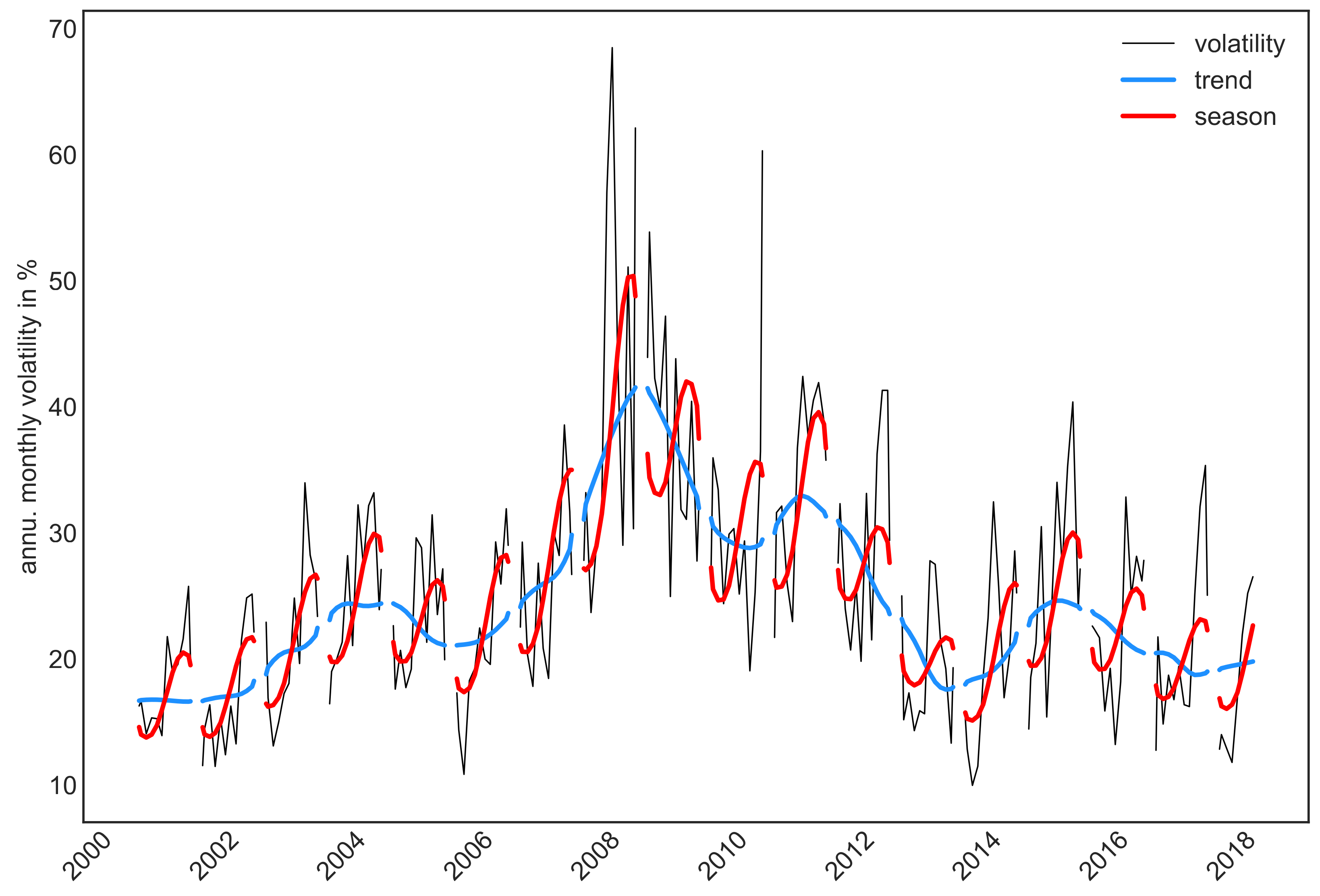
Figure 2 shows an example of the development of monthly volatility (black line) for wheat September futures contracts traded in Chicago from September 2000 to April 2018. A gap was left between each crop year (September–August) to reinforce the roll-over to the next contract visually. The estimated trend is shown in blue, and the seasonal component calculated with the $Model-ST$ is shown in red. Based on the parameters estimated in sample, the model’s plausibly depicts the underlying deterministic properties of volatility. Figure 2 shows that volatility decreases abruptly from one marketing year to the next and increases again in the following marketing year. This natural pattern is difficult to capture and calibrate using a mean reversion process.

Figure 2. Chicago Wheat—evolution of normal volatility including trend and seasonal component. The figure shows the evolution of monthly volatility (black line) for September wheat future contracts traded in Chicago, September 2000 to April 2018. A gap was left between each marketing year (September–August) to visually reinforce the roll-over to the next contract. The estimated trend is shown in blue. The estimated seasonal component is shown in red, with the respective parameter estimates belonging to the $Model-ST$; see Table 1 panel B, in red.

5.2. Storage Dynamics

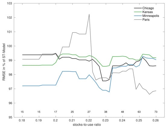
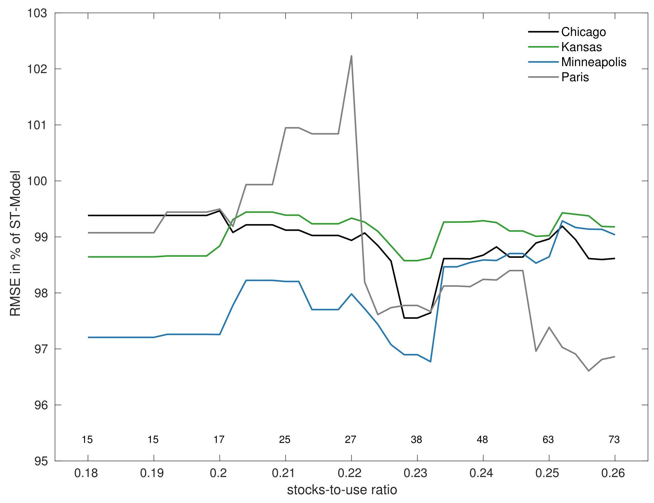
To choose a critical $stu$ level that splits our data sample into a low- and medium- to high-stock environment, we estimate the RMSEs of $Model-S$ and $Model-ST$ according to Equation (7). Figure 3 shows the $stu$-dependent RMSE development, expressed as a percentage between the fixed RMSE of $Model-ST$ and the state-dependent RMSE of $Model-S{T}_{stu}$. A value below 100% means that the $Model-S{T}_{stu}$ has a lower RMSE than the $Model-ST$.

Figure 3. RMSE comparison between $Model-ST$ and $Model-S{T}_{stu}$. The figure shows the RMSE expressed as a percentage between the $Model-ST$ and the state-depended $Model-S{T}_{stu}$. A value below 100% means that the $Model-S{T}_{stu}$ has a lower RMSE than the $Model-ST$. The RMSE $Model-S{T}_{stu}$ depends on the threshold value, i.e., the stocks-to-use ratio. The numbers above the x-axis indicate the number of observations in the subsample for which the corresponding threshold value (shown below the x-axis) was selected.

The results can be interpreted as follows: Firstly, the RMSE minimum within the selected $stu$ range is around 23% for the three US markets. For Paris, a local minimum is also 23%, with lower RSME values observed from around 25%. These findings are in line with those of [32,34], indicating that scarcity (stock-out) might be a useful indicator for calibrating state-dependent volatility parameters. Secondly, however, the in-sample decline in the RMSE is relatively small, ranging from 1% for Kansas to 3% for Minneapolis. This small, additional RMSE gain must be weighed against the additional calibration of four parameters and the threshold itself. Thirdly, the number of observations in the subsample where $stu<$ 23% is relatively low at 38. To see this, the number of observations in each subsample, which is a function of the threshold (below the x-axis), is plotted above the x-axis in Figure 3.

Following this result, we select 23% as the critical value for the $stu$ ratio.

In the next step, state-dependent seasonal volatility parameters are estimated using a threshold of 23% for the $stu$. The estimation results are summarized in Table 2, whereby the environment with low stocks is shown in the left-hand field of the table (columns 2 to 5) and the environment with high stocks in the right-hand field (columns 6 to 9).

Table 2. Seasonality and trend parameters of wheat futures’ volatility.

	Panel A: Stocks-to-Use Ratio < 23%				Panel B: Stocks-to-Use Ratio ≥ 23%
	$\mathit{\theta }$	$\mathit{\zeta }$	$\mathit{\beta }$	$\mathit{c}$	$\mathit{\theta }$	$\mathit{\zeta }$	$\mathit{\beta }$	$\mathit{c}$
Chicago	0.25 ***	−0.13 ***	0.03	0.02	0.12 ***	−0.25 ***	−0.31 ***	0.16 ***
Kansas	0.20 ***	−0.05	−0.10	0.08	0.14 ***	−0.18 ***	−0.16 ***	0.08 ***
Minneapolis	0.17 ***	−0.00	−0.22 ***	0.18 ***	0.19 ***	−0.25 ***	−0.19 ***	0.10 **
Paris	0.10 **	−0.37 ***	0.10 **	−0.03	0.14 ***	−0.39 ***	−0.40 ***	0.25 ***

The table contains estimated sine and time-to-maturity parameters, which describe the oscillation (seasonal pattern) in the volatility of September wheat futures contracts. The parameter $\theta$ represents the amplitude, i.e., the peak deviation in the function from zero; $\zeta$ represents the phase, i.e., where the oscillation is zero at time t; the constant parameter is denoted with c; and the time-to-maturity effect is captured by $\beta$. Parameters are estimated using de-trended log volatility over the period September 2000 to April 2018 and the corresponding 5%/1% levels of significance are marked with **/***, respectively.

Comparing the amplitude parameters $\theta$, the parameters are significant in both states and larger in a low inventory environment for Chicago and Kansas (see columns 2 and 6). In Minneapolis and Paris, however, the opposite is the case. While the former is consistent with the theory of storage, this is not the case for Minneapolis and Paris.

As the phase parameters are determined by the planting and harvesting time, the storage level should only have a minor influence. However, we find that $\zeta$ varies considerably between the two states, with the exception of Paris. While the estimated $\zeta$ parameters from the subsample with high $stu$ are plausible and quite similar to those of the ST model, the low-$stu$ state provides less reliable results. Similarly, the estimated time-to-maturity parameters $\beta$ in the high-$stu$ state are plausible and significant, while the opposite is found in the low-$stu$ state.

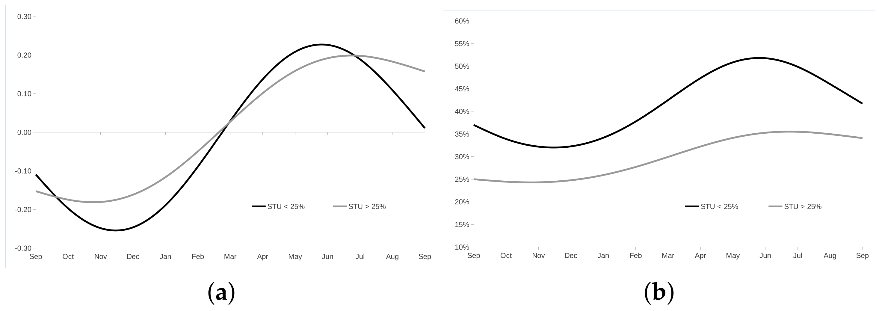
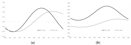
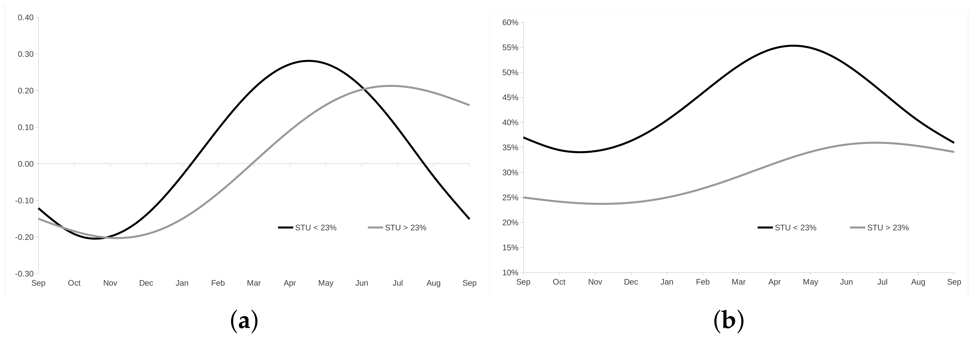
A graphical analysis, similar to Figure 1, makes it easier to check the plausibility of the parameters. Figure 4 illustrates the effect of state-dependent seasonality using the estimated parameters of Chicago wheat, presented in Table 2, with a level volatility of 37% in the low stock environment and 25% otherwise.

Figure 4. State − dependent seasonal volatility component. The figure shows the seasonal pattern of historical Chicago wheat futures’ price volatility with September expiration. The volatility development spans the season from September to August, i.e., a marketing year. Seasonal parameters are taken from Table 2, where the sample is split according to a critical stocks-to-use ratio (stu) of 23%. The annualized volatility level is set to 37% when $stu<23\%$, and 25% otherwise. The calibration window spans the period from September 2000 to April 2018. (a) Seasonal log volatility; (b) seasonal volatility with ${\overline{\sigma }}_{F\left(T\right)}=25\%$, if $stu\ge 23\%$, and ${\overline{\sigma }}_F\left(T\right)=37\%$, if $stu<23\%$.

Figure 4a shows that the seasonality in an environment with low stocks has a more pronounced amplitude (black line) with −20% and +30%; however, between November and April–May and not between winter and harvest time, as expected. In contrast, the pattern of seasonal volatility is in line with expectations of ±20% between winter and around harvest (gray line) in an environment of high inventories.

Figure 4b illustrates the effect of a larger amplitude using a volatility level of 37% analog to those observed between 2008 and 2010; see Figure 2. In a low-stock environment, volatility ranges between 32% in November and increases up to 55% in April/May (black line), showing substantial volatility spikes, however, before harvest. In contrast, in an environment of high inventories, volatility ranges only moderately between 25% and 35% (gray line), and volatility spikes around harvest.

One possible explanation for the implausible results is the low number (38) of observations in the subsample $stu$ < 23%. To test this hypothesis, we increased the $stu$ threshold to 25%, which increased the number of observations in the subsample to 63.

The results are presented in Table A1 in Appendix A, showing a much more plausible picture. The findings can be summarized as follows: Seasonality is dominated by the sinusoidal function when stocks are low, while the time-to-maturity effect is under-represented. In contrast, when stocks are adequate, the time-to-maturity effect becomes more important, while the seasonality effect decreases; see also Figure A1 in Appendix A.

Although the results are significant and plausible at a threshold of 25%, the RMSE results show that in the sample, no model improvement can be achieved with the $Model-S{T}_{stu}$ at this threshold; see Figure 3. This result clearly shows the existing challenge of a plausible parametrization of the models with an insufficient number of observations.

5.3. Out-of-Sample Model Comparison

We statistically evaluated the forecasting ability of two volatility models by applying the adjusted ref. [37] DM test according to Equation (14). The results of the pairwise tests of predictive accuracy are shown in Table 3. The table can be read as follows: A positive number means that the model in the column performs better in the out-of-sample period than the model in the row. In other words, the model in the row has a higher forecast error than the model in the column. In addition, the absolute value of the DM statistic reflects the magnitude of the difference in predictive accuracy. Larger absolute values indicate a larger difference between the forecast errors of the two models.

Table 3. Comparison of realised volatility with model forecasts and implied volatility.

Panel A: Wheat—Chicago
	$Model-ST$	$Model-S{T}_{stu}$	Implied Volatility
30-day volatility	13.95 ***	10.55 ***	17.21 ***
$Model-ST$		−11.57 ***	10.97 ***
$Model-S{T}_{stu}$			12.94 ***
Panel B: Wheat—Minneapolis
	$Model-ST$	$Model-S{T}_{stu}$	implied volatility
30-day volatility	13.78 ***	5.96 ***	10.85 ***
$Model-ST$		−15.51 ***	7.38 ***
$Model-S{T}_{stu}$			9.56 ***
Panel C: Wheat—Kansas
	$Model-ST$	$Model-S{T}_{stu}$	implied volatility
30-day volatility	11.29 ***	7.54 ***	9.17 ***
$Model-ST$		−11.49 ***	4.72 ***
$Model-S{T}_{stu}$			7.42 ***
Panel D: Wheat—Paris
	$Model-ST$	$Model-S{T}_{stu}$	implied volatility
30-day volatility	10.38 ***	8.67 ***	10.22 ***
$Model-ST$		−8.7 ***	6.1 ***
$Model-S{T}_{stu}$			7.64 ***

This table shows a comparison of the predictive performance of the applied volatility models using the modified Diebold and Mariano (1995) test statistic defined in Equation (14). A positive number indicates that the model in the column outperforms the model in the row. The forecast horizon decreases as the marketing year progresses and is 317 days at the beginning and 15 days at the end of the marketing year analyzed. The level of significance of this outperformance is marked with ***, indicating statistical significance at the 1% levels. The out-of-sample period spans from September 2013 to July 2017.

Overall, the volatility forecasts derived from implied volatility are significantly better than those of all other models examined. This result is consistent with the general view that the market’s best estimate of futures volatility is implied volatility; see [5]. In contrast, the model with constant volatility (30-day volatility) performs significantly worse than all other models. This is in line with the results of most of the literature. In contrast to the in-sample test results, among the seasonal models, the simpler $Model-ST$ provides a significantly better predictive performance than the more sophisticated $Model-S{T}_{stu}$ with two states. This result indicates an overfitting problem of the in-sample test, especially due to the low number of observations for the state with low stocks-to-use ratios.

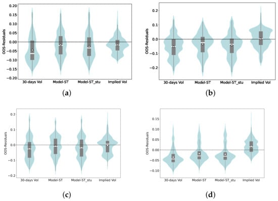
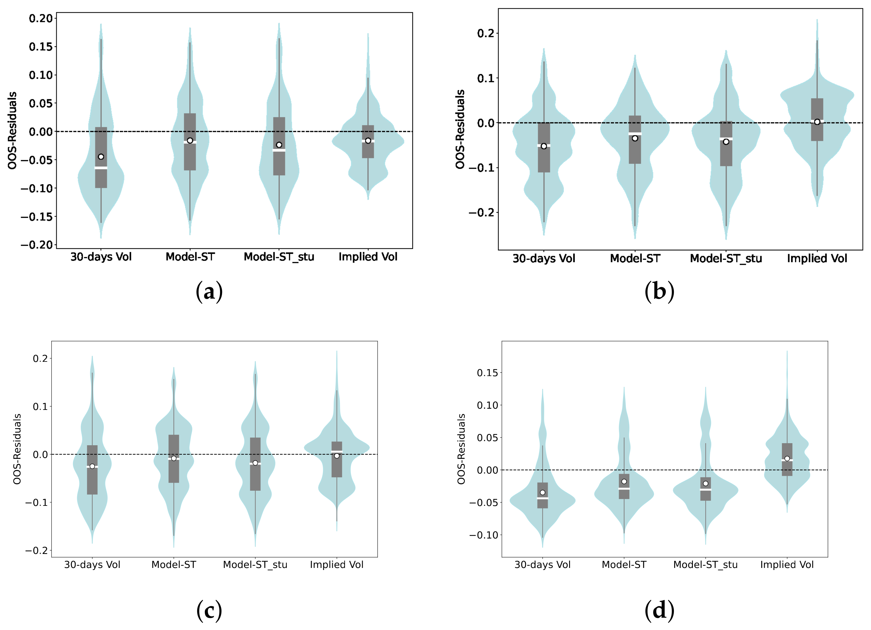
The distribution of the residuals of the out-of-sample test provides additional visual information about the average of the errors made and their dispersion. We use violin diagrams that visually compare the residual distribution for each model and highlight skewness, multimodality, and outliers.

Figure 5 contains the violin plots, where subplots (a) to (d) represent the four markets, and each subplot shows the distribution of the forecast errors of the four models. The white horizontal bar in each violin plot shows the median, and the white dot is the mean forecast error. Models with violin plots more centered around the black dashed line, representing zero residuals, are performing better, indicating that their predictions are closer to the actual values.

Figure 5. Model comparison of forecast errors. The figure shows violin plots for out-of-sample forecast errors. The out-of-sample period spans from September 2013 to July 2017. Subplots (a–d) represent the four markets, and each subplot shows the distribution of the forecast errors of the four models. The white horizontal bar in each violin plot shows the median, the white dot is the mean forecast error, and the black dashed line represents zero residuals. (a) Chicago; (b) Minneapolis; (c) Kansas; (d) Paris.

Overall, the visualization of the prediction errors supports the results from the DM test statistics. In particular, the mean forecast errors (white dot) for the implied volatility are close to zero; this also applies partly to the $Model-ST$, see Chicago and Kansas. However, the distribution of implied volatility forecast errors is more strongly centered around zero than all other models. All models underestimated the realized volatility in nearly all cases, with mean and median forecast errors below zero. Consistent with existing literature, implied volatility is close to realized volatility in Minneapolis and Kansas and above the realized volatility in Paris. The only exception to this pattern is Chicago.

Although existing literature empirically demonstrates that implied volatility often overestimates realized volatility, as evidenced by negative variance risk premiums found in [40] in the crude oil market and in [41] in four energy markets, our findings align with those of [42]. (The variance risk premium of a variance swap is determined by the difference between realized volatility and implied volatility. When realized volatility exceeds implied volatility, the variance swap yields a positive risk premium, and vice versa.) The authors documented positive variance risk premiums for only 3 out of 27 commodities, including wheat, in the post-2001 period of their subsample. Refs. [41,43] found that variance risk premiums are highly time-varying; they are often negative at short maturities and positive at long maturities, although the maturity patterns are not very strong.

However, it appears implausible that the option’s maturity alone explains the underestimation of realized volatility by implied volatility exclusively for Chicago, given that the options’ maturities are consistent across all markets in our sample.

Another explanation for this result could be related to the financialization of commodity markets, particularly due to varying degrees of speculative activity on commodity exchanges. Ref. [41] demonstrated that producers are net-short of the underlying through their option positions in the energy market, while speculators are net-long. The larger the net-long position of speculators, the lower the returns on call options, and vice versa.

Similar to [44], which examined growth options in the stock market, this study found that the expected profitability of selling options has diminished due to increased competition and the growing popularity of retail options trading, squeezing profitability margins for traditional option sellers.

Following both arguments and assuming that speculators act as insurers through the net sale of options, the results in Chicago suggest an oversupply of options during the observation period, leading to a low market price of risk. (The groundwork for understanding how implied volatility incorporates both market expectations of futures volatility and the market price of risk is given in [45,46].) On the other hand, the opposite may have been the case in Paris, with too little supply leading to a high market price of risk.

A further explanation for the cross-sectional differences in our sample is related to market liquidity. Ref. [47] identified a positive illiquidity premium for equity options that compensates market makers for the risks and costs of holding large and risky net-long positions. Chicago is known for its high liquidity, followed by Kansas and Minneapolis, while Paris has the lowest market liquidity [26].

Parameter Stability

In the following, we examine the parameter stability for $Model-ST$, as this has the best out-of-sample property of the volatility models. The aim is to make a statement about how robust the parameters are for a market over time and to what extent the parameters differ between the markets over time. Estimated parameters can be transferred from liquid markets to illiquid markets if the parameter stability is given.

We use the estimated parameters from the calibration period of the out-of-sample test, in which the parameters are calibrated based on monthly observations in a rolling window of 13 years. The first calibration window covers the period from September 2000 to August 2013, and the last window covers the period from June 2004 to June 2017, resulting in 47 periods.

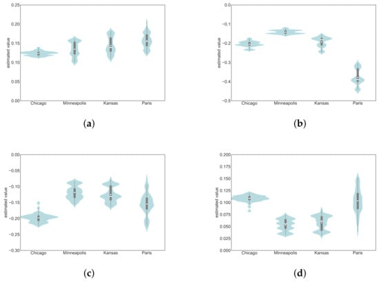
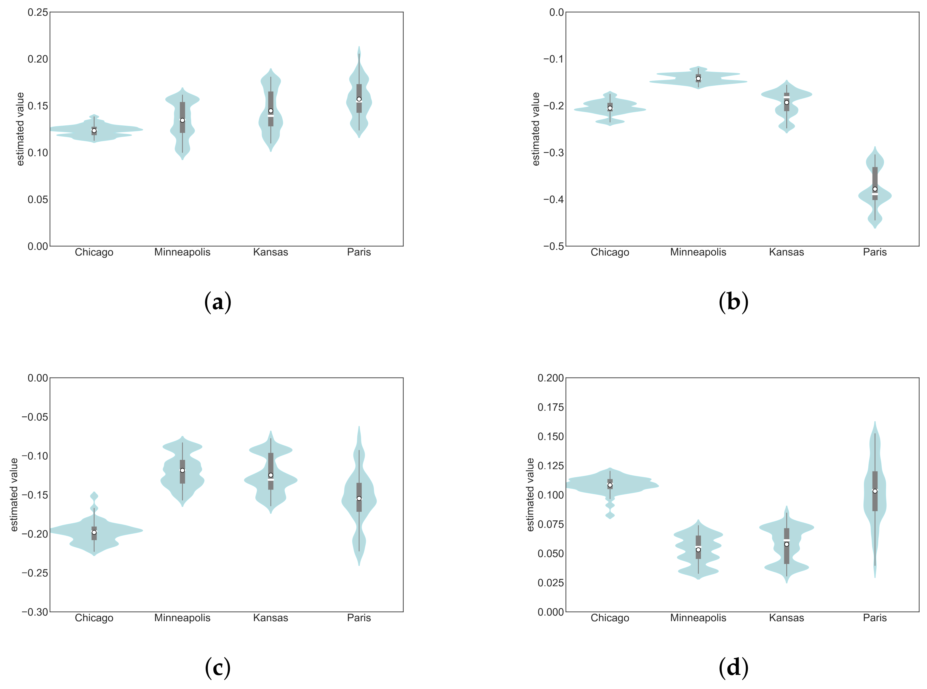
Figure 6 shows the violin plot for rolling estimated parameters: amplitude, phase, time to maturity, and constant. Subplots (a) to (d) represent the four parameters, and each subplot shows the parameter distribution for one of the four markets, namely Chicago, Minneapolis, Kansas, and Paris. The white horizontal bar in each violin plot shows the median, and the white dot shows the sample mean. Starting with the amplitude, in Figure 6a, the mean and median are very narrow across the four markets analyzed. While the distribution of the amplitude parameters in Chicago is most strongly centered around the mean, all other markets show a similar distribution. This result indicates that the amplitude parameter can be regarded as stable both over time and between markets.

Figure 6. Parameter stability. The figure shows the violin plot for rolling estimated parameters, namely amplitude, phase, time to maturity, and constant. Subplots (a–d) represent the four parameters, and each subplot shows the parameter distribution for one of the four markets, namely Chicago, Minneapolis, Kansas, and Paris. The white horizontal bar in each violin plot shows the median, and the white dot shows the sample mean. The parameters are calibrated based on monthly observations in a rolling window of 13 years. The first calibration window covers the period from September 2000 to August 2013, and the last one covers the period from June 2004 to June 2017, resulting in a total of 47 periods. (a) Amplitude; (b) phase; (c) time to maturity; (d) constant.

We find a similar result for the phase parameter, Figure 6b, with the exception of Paris, which differs significantly from its US counterparts. However, this parameter can be selected or checked for plausibility with regard to the respective harvest cycle.

The distribution characteristics for the maturity parameters, shown in Figure 6c, are very similar for Minneapolis, Kansas, and Paris, but Chicago has a higher value and the distribution is more centered. However, the signs remain stable. A similar picture emerges for the constant, as shown in Figure 6d. This indicates that a corresponding tolerance is considered when transferring the parameters to other markets.

6. Black’s Option Pricing Model Extension

In the following sections, we demonstrate that the presented volatility models can be integrated into the option pricing model of [6] for options on futures, with a focus on the closed-form solutions available for European options. European options have a distinct characteristic in that they can only be exercised at expiration. In contrast, American-style options, which are more commonly used, can be exercised at any time until expiration. Ref. [48] provides an analytical approximation for American option values, but the method relies on numerical solutions. For further details, readers are referred to [5], page 97 ff.

While the model of [6] uses a constant volatility, we followed the idea of [18] or [19], and replaced the constant volatility $\sigma$ with the deterministic time varying volatility ${\sigma }_s$ as described by Equation (3). Hence, the price dynamic under the risk neutral measure is given by

$$\begin{array}{ccc}\hfill d{F}_t& =& F_t{\sigma }_{s,t}d{Z}_t^Q,\hfill \\ & =& F_t\overline{\sigma }{e}^{\phi \left(t\right)}d{Z}_t^Q,\hfill \end{array}$$

(15)

with

$$\phi \left(t\right)=\theta \sin \left(2\pi \right(t+\zeta \left)\right),$$

(16)

where $\overline{\sigma }$ denotes the volatility level, which is assumed to be constant over the option’s life time. The sinusoidal function, which describes the deterministic behavior around the future’s volatility level, is represented by $\phi \left(t\right)$, where $\theta$ denotes the amplitude parameter, i.e., the peak deviation of the function from zero, and $\zeta$ denotes the respective phase parameter, i.e., where the oscillation is zero at time t. The following model extension accounts for the time-to-maturity effect:

$$\phi \left(t\right)=c+\beta (T-t)+\theta \sin \left(2\pi \right(t+\zeta \left)\right),$$

(17)

where the constant c and $\beta$ captures the impact of decreasing time to maturity, and $T-t$ reflects the time to expiration. The seasonal and time-to-maturity parameters can be calibrated to historical data or to the subjective beliefs of a trader.

The European call option price C is calculated using the standard Black’s formula by accounting for a deterministic time varying volatility ${\sigma }_s$ according to

$${\sigma }_s=\sqrt{{\displaystyle \frac{1}{T-t}}{\int }_t^T{\overline{\sigma }}^2{e}^{2\phi \left(t\right)}dt}=\overline{\sigma }\sqrt{{\displaystyle \frac{1}{T-t}}{\int }_t^T{e}^{2\phi \left(t\right)}dt},$$

(18)

where $\overline{\sigma }$ denotes the volatility level. The integral can be solved numerically, e.g., with Romberg’s method or the trapezoid rule. Finally, the price for a call C and a put P option is then given by

$$\begin{array}{ccc}\hfill C& =& e^{-r(T-t)}\left[FN\left(d_1\right)-KN\left(d_2\right)\right],\hfill \end{array}$$

(19)

$$\begin{array}{ccc}\hfill P& =& e^{-r(T-t)}\left[KN(-d_2)-FN(-d_1)\right],\hfill \end{array}$$

(20)

with

$$\begin{array}{ccc}\hfill d_1& =& {\displaystyle \frac{ln\left(\frac{F}{K}\right)+\frac{{\overline{\sigma }}^2}{2}{\int }_t^T{e}^{2\phi \left(t\right)}dt}{\overline{\sigma }\sqrt{{\int }_t^T{e}^{2\phi \left(t\right)}dt}}},\hfill \\ \hfill d_2& =& {\displaystyle \frac{ln\left(\frac{F}{K}\right)-\frac{{\overline{\sigma }}^2}{2}{\int }_t^T{e}^{2\phi \left(t\right)}dt}{\overline{\sigma }\sqrt{{\int }_t^T{e}^{2\phi \left(t\right)}dt}}}\hfill \\ & =& d_1-\overline{\sigma }\sqrt{{\int }_t^T{e}^{2\phi \left(t\right)}dt}.\hfill \end{array}$$

where r denotes the risk-free interest rate, and $N(·)$ stands for the cumulative normal distribution function.

7. Conclusions

Accurately pricing options on wheat futures is crucial for participants in agricultural markets, including traders, insurers, and policymakers. The distinct characteristics of wheat futures, influenced by seasonality, time to maturity, and storage dynamics, pose significant challenges for traditional option pricing models like the Black (1976) model, which assumes constant volatility and fails to capture the systematic variations in wheat futures markets.

This study addresses the gap between traditional volatility models and more sophisticated models that require large datasets. We provide a robust model that captures the dynamics of wheat futures volatility with only a few calibratable parameters, ensuring that the estimated volatility pattern aligns with the harvest cycle.

Unlike models with numerous estimated parameters, our approach minimizes error-proneness and facilitates plausibility checks, reducing the risk of using unspecified models. Additionally, our model allows for an economic interpretation of parameters, which is often challenging with other sophisticated models.

We incorporate seasonal patterns, the time-to-maturity effect, and storage dynamics through the U.S. stocks-to-use ratio. While the stocks-to-use ratio may be unsuitable for predicting volatility when shortages rarely occur during the calibration period, it can be useful for risk modeling. With some limitations, estimated parameters can be transferred from liquid markets to similar illiquid markets, a task that is difficult for more sophisticated models requiring a large number of parameters. This application has significant implications, such as for crop failure insurance, and offers practical relevance for market participants by providing a more effective tool for modeling volatility in illiquid markets. Additionally, the introduced volatility model is suitable for pricing European options on wheat futures in a risk-neutral measure.

References

- Natoli, F. Financialization of commodities before and after the great financial crisis. J. Econ. Surv. 2021, 35, 488–511. [Google Scholar] [CrossRef] [Scilit]
- Haase, M.; Zimmermann, Y.S.; Zimmermann, H. The impact of speculation on commodity futures markets—A review of the findings of 100 empirical studies. J. Commod. Mark. 2016, 3, 1–15. [Google Scholar] [CrossRef] [Scilit]
- Foucault, T.; Pagano, M.; Röell, A. Market Liquidity: Theory, Evidence, and Policy; Oxford University Press: Oxford, MS, USA, 2013. [Google Scholar]
- Brunnermeier, M.K.; Pedersen, L.H. Market liquidity and funding liquidity. Rev. Financ. Stud. 2009, 22, 2201–2238. [Google Scholar] [CrossRef] [Scilit]
- Haug, E.G. Option Pricing Formulas; McGraw-Hill: New York, NY, USA, 2007. [Google Scholar]
- Black, F. The pricing of commodity contracts. J. Financ. Econ. 1976, 3, 167–179. [Google Scholar] [CrossRef] [Scilit]
- Samuelson, P.A. Proof that properly anticipated prices fluctuate randomly. In The World Scientific Handbook of Futures Markets; World Scientific: Singapore, 2016; pp. 25–38. [Google Scholar]
- Anderson, R.W.; Danthine, J.P. The time pattern of hedging and the volatility of futures prices. Rev. Econ. Stud. 1983, 50, 249–266. [Google Scholar] [CrossRef] [Scilit]
- Choi, J.W.; Longstaff, F.A. Pricing options on agricultural futures: An application of the constant elasticity of variance option pricing model. J. Futur. Mark. 1985, 5, 247. [Google Scholar] [CrossRef] [Scilit]
- Boos, D. Risky times: Seasonality and event risk of commodities. J. Futur. Mark. 2024, 5, 767–783. [Google Scholar] [CrossRef] [Scilit]
- Fackler, P.L.; Tian, Y. Volatility models for commodity markets. In Proceedings of the NCR-134 Conference on Applied Commodity Price Analysis, Forecasting, and Market Risk Management, Chicago, IL, USA, 19–20 April 1999; pp. 247–256. [Google Scholar]
- Sørensen, C. Modeling seasonality in agricultural commodity futures. J. Futur. Mark. Futur. Options Other Deriv. Prod. 2002, 22, 393–426. [Google Scholar] [CrossRef] [Scilit]
- Schwartz, E.; Smith, J.E. Short-term variations and long-term dynamics in commodity prices. Manag. Sci. 2000, 46, 893–911. [Google Scholar]
- Schneider, L.; Tavin, B. Seasonal volatility in agricultural markets: Modelling and empirical investigations. Ann. Oper. Res. 2024, 334, 7–58. [Google Scholar] [CrossRef] [Scilit]
- Brennan, M.J. The Supply of Storage. Am. Econ. Rev. 1958, 48, 50–72. [Google Scholar]
- Williams, J.; Wright, B. Storage and Commodity Markets; Cambridge University Press: Cambridge, UK, 1991. [Google Scholar]
- Deaton, A.; Laroque, G. Competetive Storage and Commodity Price Dynamics. J. Political Econ. 1996, 104, 896–923. [Google Scholar] [CrossRef] [Scilit]
- Geman, H.; Nguyen, V.N. Soybean Inventory and Forward Curve Dynamics. Manag. Sci. 2005, 51, 1076–1091. [Google Scholar] [CrossRef] [Scilit]
- Back, J.; Prokopczuk, M.; Rudolf, M. Seasonality and the valuation of commodity options. J. Bank. Financ. 2013, 37, 273–290. [Google Scholar] [CrossRef] [Scilit]
- Richter, M.; Sørensen, C. Stochastic Volatility and Seasonality in Commodity Futures and Options: The Case of Soybeans. Work. Pap. 2005, 51, 1076–1091. [Google Scholar] [CrossRef] [Scilit]
- Koekebakker, S.; Lien, G. Volatility and price jumps in agricultural futures prices?evidence from wheat options. Am. J. Agric. Econ. 2004, 86, 1018–1031. [Google Scholar] [CrossRef] [Scilit]
- Bates, D.S. The Crash of ’87: Was It Expected? The Evidence from Options Markets. J. Financ. 1991, 46, 1009–1044. [Google Scholar] [CrossRef] [Scilit]
- Arismendi, J.C.; Back, J.; Prokopczuk, M.; Paschke, R.; Rudolf, M. Seasonal stochastic volatility: Implications for the pricing of commodity options. J. Bank. Financ. 2016, 66, 53–65. [Google Scholar] [CrossRef] [Scilit]
- Miltersen, K.R.; Schwartz, E.S. Pricing of options on commodity futures with stochastic term structures of convenience yields and interest rates. J. Financ. Quant. Anal. 1998, 33, 33–59. [Google Scholar] [CrossRef] [Scilit]
- Czudaj, R.L. Dynamics between trading volume, volatility and open interest in agricultural futures markets: A Bayesian time-varying coefficient approach. Econom. Stat. 2019, 12, 78–145. [Google Scholar] [CrossRef] [Scilit]
- Haase, M.; Huss, M. Guilty speculators? Range-based conditional volatility in a cross-section of wheat futures. J. Commod. Mark. 2018, 10, 29–46. [Google Scholar] [CrossRef] [Scilit]
- Janzen, J.P.; Adjemian, M.K. Estimating the location of world wheat price discovery. Am. J. Agric. Econ. 2017, 99, 1188–1207. [Google Scholar] [CrossRef] [Scilit]
- Corrado, C.; Miller, T. A note on a simple, accurate formula to compute implied standard deviations. J. Bank. Financ. 1996, 20, 595–603. [Google Scholar] [CrossRef] [Scilit]
- Bunek, G.D. Characterizing the Effect of USDA Report Announcements in the Winter Wheat Futures Market Using Realized Volatility. Ph.D. Thesis, Montana State University-Bozeman, College of Agriculture, Bozeman, MT, USA, 2015. [Google Scholar]
- Lehecka, G.V.; Wang, X.; Garcia, P. Gone in ten minutes: Intraday evidence of announcement effects in the electronic corn futures market. Appl. Econ. Perspect. Policy 2014, 36, 504–526. [Google Scholar] [CrossRef] [Scilit]
- Vogel, F.A. Understanding USDA Crop Forecasts; National Agricultural Statistics Service and Office of the Chief Economist, World Agricultural Outlook Board: Paris, France, 1999; p. 1554. [Google Scholar]
- Chatnani, N.N. Commodity Markets: Operations, Instruments, and Applications; Tata McGraw Hill Education Private Limited: New York, NY, USA, 2010. [Google Scholar]
- Cleveland, W.S. LOWESS: A program for smoothing scatterplots by robust locally weighted regression. Am. Stat. 1981, 35, 54. [Google Scholar] [CrossRef] [Scilit]
- Bobenrieth, E.; Wright, B.; Zeng, D. Stocks-to-use ratios and prices as indicators of vulnerability to spikes in global cereal markets. Agric. Econ. 2013, 44, 43–52. [Google Scholar] [CrossRef] [Scilit]
- Greb, F.; Prakash, A. Assessing Volatility Patterns in Food Crops; No. 35, FAO commodity and trade policy research working paper series; Food and Agriculture Organization of the United Nations: Rome, Italy, 2017. [Google Scholar]
- Christoffersen, P.; Jacobs, K. The importance of the loss function in option valuation. J. Financ. Econ. 2004, 72, 291–318. [Google Scholar] [CrossRef] [Scilit]
- Diebold, F.X.; Mariano, R.S. Com paring predictive accu racy. J. Bus. Econ. Stat. 1995, 13, 253–263. [Google Scholar] [CrossRef] [Scilit]
- Harvey, D.; Leybourne, S.; Newbold, P. Testing the equality of prediction mean squared errors. Int. J. Forecast. 1997, 13, 281–291. [Google Scholar] [CrossRef] [Scilit]
- Samuelson, P.A. Proof That Properly Anticipated Prices Fluctuate Randomly. Ind. Manag. Rev. 1965, 6, 41–49. [Google Scholar]
- Kang, S.B.; Pan, X.N. Commodity variance risk premia and expected futures returns: Evidence from the crude oil market. SSRN 2015, 2296932. [Google Scholar] [CrossRef] [Scilit]
- Jacobs, K.; Li, B. Option returns, risk premiums, and demand pressure in energy markets. J. Bank. Financ. 2023, 146, 106687. [Google Scholar] [CrossRef] [Scilit]
- Prokopczuk, M.; Symeonidis, L.; Simen, C.W. Variance risk in commodity markets. J. Bank. Financ. 2017, 81, 136–149. [Google Scholar] [CrossRef] [Scilit]
- Dew-Becker, I.; Giglio, S.; Kelly, B. Hedging macroeconomic and financial uncertainty and volatility. J. Financ. Econ. 2021, 142, 23–45. [Google Scholar] [CrossRef] [Scilit]
- Bali, T.G.; Del Viva, L.; Lambertides, N.; Trigeorgis, L. Growth options and related stock market anomalies: Profitability, distress, lotteryness, and volatility. J. Financ. Quant. Anal. 2020, 52, 2150–2180. [Google Scholar] [CrossRef] [Scilit]
- Black, F.; Scholes, M. The pricing of options and corporate liabilities. J. Political Econ. 1973, 81, 637–654. [Google Scholar] [CrossRef] [Scilit]
- Merton, R.C. An intertemporal capital asset pricing model. Econom. J. Econom. Soc. 1973, 41, 867–887. [Google Scholar] [CrossRef] [Scilit]
- Christoffersen, P.; Goyenko, R.; Jacobs, K.; Karoui, M. Illiquidity premia in the equity options market. Rev. Financ. Stud. 2018, 31, 811–851. [Google Scholar] [CrossRef] [Scilit]
- Barone-Adesi, G.; Whaley, R.E. Efficient analytic approximation of American option values. J. Financ. 1987, 42, 301–320. [Google Scholar] [CrossRef]
Disclaimer/Publisher’s Note: The statements, opinions and data contained in all publications are solely those of the individual author(s) and contributor(s) and not of MDPI and/or the editor(s). MDPI and/or the editor(s) disclaim responsibility for any injury to people or property resulting from any ideas, methods, instructions or products referred to in the content. |
© 2024 by the authors. Licensee MDPI, Basel, Switzerland. This article is an open access article distributed under the terms and conditions of the Creative Commons Attribution (CC BY) license (https://creativecommons.org/licenses/by/4.0/).