Who Can Afford to Buy a Home? Tourism Pressure and Profile-Based Housing Purchase Opportunities in Italian Cities

Abstract

This study examines simulated mortgage-financed home-purchase opportunities across ten Italian cities from 2008 to 2024 in relation to tourism intensity, residential prices, local incomes and mortgage conditions. The unbalanced estimation sample includes 160 city-year observations, generating 960 deterministic scenarios for six representative household profiles. Price-to-income ratios, mortgage burdens and a Housing Opportunity Index are used to characterise these scenarios. Two-way fixed-effects models estimate city-year associations, while Random Forest and Histogram Gradient Boosting assess out-of-sample prediction under temporal and leave-one-city-out validation. At an assumed 30% mortgage-burden threshold, 64.4% of scenarios for young couples and higher-income households are classified as affordable, compared with 31.3% for young singles and 17.5% for tourism-sector workers. In the reported fixed-effects specifications, municipal income is positively associated with residential prices (β = 3.896; p = 0.033), whereas tourism intensity is not statistically significant in either the price (β = −0.147; p = 0.528) or price-to-income model (β = −0.088; p = 0.677). Random Forest performs well under temporal validation (R² = 0.742) but not when transferred to an unseen city (R² = −0.292). These percentages represent scenario frequencies, not shares of actual residents. The reconstructed tourism series and small number of cities limit statistical inference and do not support causal claims about tourism or conclusions regarding rental affordability.

1. Introduction

Are cities still places in which residents can build their lives, or are urban housing markets increasingly organised around temporary consumption and real-estate returns? This tension is especially evident in tourism-intensive cities, where dwellings simultaneously function as homes, investment assets, second residences and short-term accommodation. Although tourism may support employment, investment and urban regeneration, concentrated visitor demand may increase property values and encourage the conversion of residential units, particularly where housing supply is spatially constrained [1,2,3]. Digital platforms have intensified this process by reducing the costs of placing housing on the tourist market and increasing the expected returns from short-term rentals [4].

Nevertheless, rising property prices do not necessarily imply declining affordability. Tourism may also increase local employment and income, partially compensating residents for higher housing costs. Purchase affordability may deteriorate when house prices and financing costs rise faster than household resources, particularly when the benefits of tourism accrue mainly to property owners and investors while wages remain low or seasonal [5]. The relevant issue is therefore not property appreciation alone, but whether different resident groups retain effective access to urban housing.

Recent national developments make the relationship between tourism and housing access particularly relevant in Italy. In 2024, the final year of the study period, registered accommodation establishments recorded 139.6 million tourist arrivals and 466.2 million overnight stays; overnight stays increased by 4.2% compared with 2023 [6]. In the same year, the national House Price Index rose by an annual average of 3.2% [7]. These concurrent trends do not establish that tourism caused the increase in housing prices. They nevertheless highlight the need to examine whether households with different resources face comparable home-purchase opportunities in cities exposed to varying levels of visitor demand.

National price trends cannot capture conditions in individual urban markets, and property prices alone cannot establish whether a household can finance a purchase. The relevant comparison also depends on local income, the size of the dwelling required, mortgage interest rates and the assumed down payment [8].

Existing studies have mainly examined associations between tourism or short-term rentals and residential prices or rents [1,4,5]. Comparative evidence on how local prices, incomes and mortgage assumptions translate into different purchase scenarios across Italian cities remains limited, particularly for periods before and after the pandemic. The present analysis therefore distinguishes descriptive household scenarios from city-year econometric associations and out-of-sample prediction.

This study examines how common city-level prices, income proxies and mortgage conditions translate into different simulated home-purchase opportunities for six representative household profiles across ten Italian cities. Its contribution is threefold. First, it compares mortgage-financed purchase scenarios rather than interpreting property appreciation as an affordability measure. Second, it documents differences among household profiles and cities while explicitly stating the assumptions underlying those comparisons. Third, it combines two-way fixed-effects estimates with exploratory nonlinear models and out-of-sample machine-learning validation, distinguishing descriptive scenarios, statistical associations and prediction. It does not identify causal, group-specific tourism effects.

The main research question is:

How do local housing-market conditions and predefined household characteristics shape simulated mortgage-financed home-purchase opportunities across Italian cities, and is tourism intensity associated with city-year prices or price-to-income conditions?

Specifically, the study examines the following sub-questions:

RQ1: How do simulated home-purchase opportunities vary across the selected cities and available years between 2008 and 2024?

RQ2: Is tourism intensity associated with residential prices and price-to-income conditions after controlling for municipal income, city characteristics and common annual shocks?

RQ3: How do simulated purchase opportunities differ across the six household profiles, cities and assumed mortgage-burden thresholds?

Section 2 reviews the literature. Section 3 describes the data and methods; Section 4 presents the results; Section 5 discusses their interpretation and limitations; and Section 6 concludes.

2. Literature Review

Tourism influences housing markets through several interconnected channels, including employment and income generation, urban amenities, investment demand and the reallocation of the existing housing stock. Visitor expenditure can support local businesses, stimulate regeneration and improve public spaces, services and the external image of destinations. These benefits may be capitalised into land and property values. At the same time, tourism expands housing demand beyond the resident population by attracting second-home buyers, external investors and operators seeking returns from visitor accommodation. Where housing supply is relatively inelastic, as in historic centres, coastal destinations and heritage cities, this additional demand can generate substantial price pressures.

Italian evidence suggests that the relationship between tourism and residential prices varies across destinations. Biagi et al. [1] found a positive average association between tourism and house prices in Italian cities; their latent-class analysis identified differences by destination and local market characteristics [2]. This heterogeneity suggests that a single national coefficient may conceal substantial variation across cities. More recent cross-country evidence also examines short- and long-term links between tourism activity and housing prices in tourism-dependent economies [3].

Short-term rental platforms constitute a major transmission mechanism between demand and residential markets. By lowering information and transaction costs, platforms increase the profitability and flexibility of converting dwellings from long-term residential use to temporary accommodation. Barron et al. [4] showed that Airbnb expansion increased both rents and house prices in the United States, with larger effects in areas characterised by lower owner-occupancy rates. Wachsmuth and Weisler [5] similarly argued that Airbnb creates a new form of rent gap by allowing owners to capture tourism-derived revenues that exceed conventional residential rents.

Short-term rentals may affect residential markets when owners allocate existing dwellings to visitor accommodation rather than long-term residential use. The potential effect depends on the scale and location of conversions, the availability of alternative housing, local regulation and the responsiveness of new supply. Tourism may also support employment and income, so a price increase does not necessarily imply an equal deterioration in purchase affordability for every household.

Evidence from European cities helps clarify the spatial dimension of short-term rentals. Using neighbourhood-level data for Barcelona, Garcia-López et al. [9] found increases in rents and house prices associated with Airbnb activity, with larger estimated effects where platform activity was concentrated. Reichle et al. [10], examining 25 European cities, likewise documented effects concentrated mainly in city centres, alongside effects elsewhere within cities. Municipal tourism totals can therefore conceal differences across residential submarkets.

The concepts of touristification and tourism gentrification describe transformations extending beyond property prices. Tourism growth can alter retail structures and public-space use. Cocola-Gant [11] conceptualised these processes through place-based displacement, showing that residents may experience loss of belonging, local networks and everyday services even when they are not physically displaced. Evidence from Naples illustrates how tourism-related reinvestment can produce geographically concentrated displacement pressures within a historic urban centre [12].

This perspective is consistent with the right to adequate housing, which includes affordability alongside availability, security of tenure and habitability [13].

Housing affordability expresses the relationship between housing costs and household resources. High property prices need not indicate poor affordability when local incomes are also high, whereas comparatively inexpensive cities may still be inaccessible to households with low or unstable earnings. Mikulić et al. [14] provide a relevant empirical precedent by examining tourism activity and housing affordability across Croatian municipalities. Their findings indicate that accommodation intensity, tourism concentration, seasonality and economic dependence may operate through property-price and income channels. Tourism may strengthen purchasing capacity through employment and revenues, but these benefits need not compensate for housing appreciation in highly specialised destinations.

Italian evidence further highlights within-city heterogeneity. Congiu et al. [15] examined Airbnb density, sale prices and rents across five Italian cities, identifying variation in estimated price effects both between cities and between central and peripheral neighbourhoods. Their analysis uses a finer spatial scale than the present city-year panel. The current study instead compares explicitly defined mortgage-financed purchase scenarios and cannot identify the effects of Airbnb on individual households.

Econometric analysis and machine-learning prediction answer different questions. As discussed by Mullainathan and Spiess [16], econometric estimates focus on conditional associations and statistical inference, whereas predictive models assess performance on observations not used for model fitting. Accordingly, the fixed-effects specifications below describe within-city relationships, while Random Forest and Histogram Gradient Boosting are evaluated using temporal and leave-one-city-out validation. Predictive accuracy does not establish causation.

The literature establishes plausible relationships between tourism, short-term accommodation and residential prices or rents [1,2,3,4,5,9,10,15], and provides precedents for studying housing affordability alongside tourism [14]. The narrower contribution here is a transparent city-and-profile comparison of simulated home-purchase opportunities, accompanied by exploratory city-year models. Because the household profiles are deterministic and the tourism data are largely reconstructed, neither differentiated causal tourism effects nor the share of actual households able to purchase a dwelling can be inferred.

3. Materials and Methods

3.1. Case Study and Variables

The empirical analysis covers ten Italian cities between 2008 and 2024: Milan, Rome, Turin, Naples, Bologna, Florence, Venice, Bergamo, Reggio Emilia and Salerno. The first seven are metropolitan-city capitals, whereas Bergamo, Reggio Emilia and Salerno represent non-metropolitan urban markets. Together, these cities represent different urban scales, levels of tourism intensity and housing-market conditions.

The initial database contains 204 potential city-year records for 12 cities over 2008–2024. Bari and Genoa were excluded because their available residential-price series did not meet the temporal comparability requirement. The final unbalanced estimation sample contains 160 of 170 possible city-year observations across ten cities. Table A1 reports the missing observations by city, and Table A2 describes the source status of tourism observations.

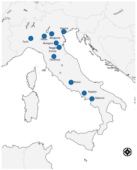
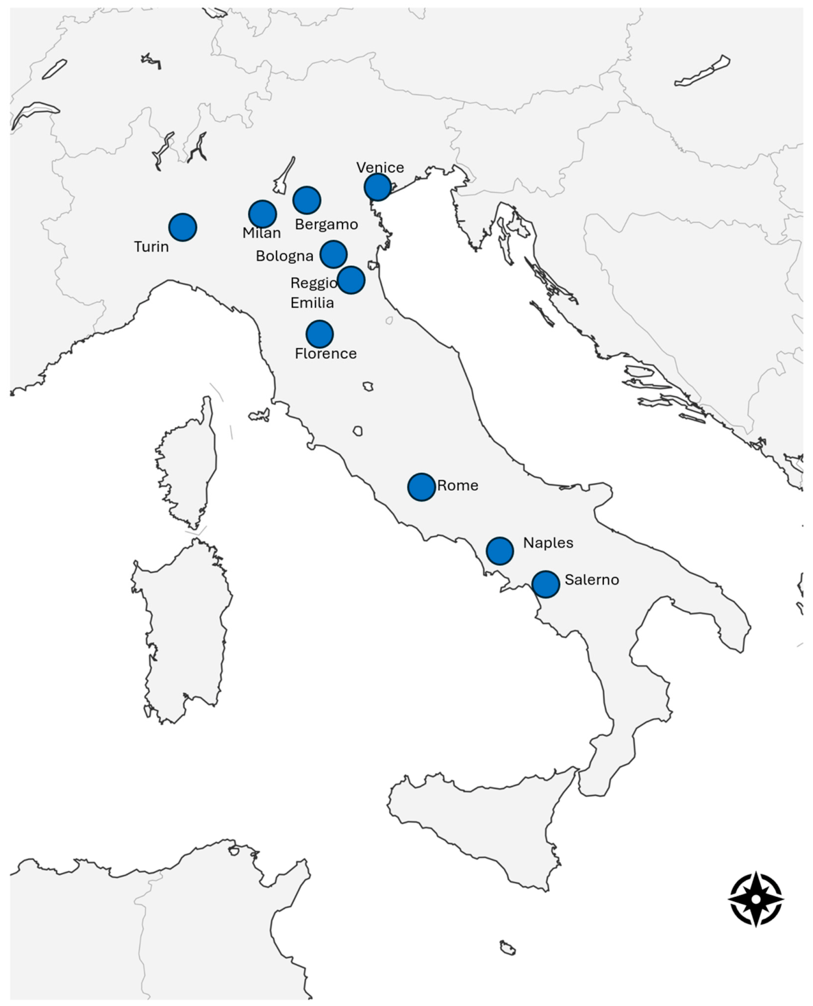
Housing-market quotations were obtained from the Italian Revenue Agency’s Real Estate Market Observatory (OMI) [17]. The principal residential-price variable is an arithmetic mean of available quotations for selected central or station-area residential submarkets within each city-year, expressed in euros per square metre. OMI quotations are neither individual transaction prices nor averages for the full municipal market. Nominal values enter the mortgage-financed purchase scenarios. A city-by-city inventory of selected OMI zones and quotation types would be necessary for full reproducibility. Municipal mean taxable income is obtained from the Italian Ministry of Economy and Finance [18], and the year-specific national mortgage-rate series is obtained from the ECB [19]. Figure 1 shows the location of the ten selected cities.

Figure 1. Location of the ten cities included in the analytical sample.

Tourism indicators are based on registered accommodation statistics [20]. These data describe municipal arrivals, overnight stays, accommodation establishments and tourist beds. They do not separately identify Airbnb listings, residential conversions or unregistered accommodation; tourism intensity is therefore not a direct measure of platform penetration.

The principal tourism-pressure indicator is the number of registered overnight stays per resident, as defined in Equation (1):

$${\mathrm{TI}}_{\mathrm{it}} = {\displaystyle \frac{{\mathit{OvernightStays}}_{\mathit{it}}}{{\mathit{Population}}_{\mathit{it}}}}$$

(1)

Here TI_it denotes annual registered overnight stays divided by the resident population of city i in year t.

Additional indicators capture complementary dimensions of tourism pressure as described by Equation (2):

$${\mathrm{AI}}_{\mathrm{it}} ={\displaystyle \frac{{\mathit{Arrivals}}_{\mathit{it}}}{{\mathit{Population}}_{\mathit{it}}}} \mathrm{and} {\mathrm{BC}}_{\mathrm{it}} ={\displaystyle \frac{{\mathit{TouristBeds}}_{\mathit{it}}}{{\mathit{Population}}_{\mathit{it}}}}\times 1000$$

(2)

Arrival intensity (AI_it) is defined as tourist arrivals per resident, while bed-capacity pressure (BC_it) is defined as tourist bed places per 1000 residents.

Arrival intensity and bed-capacity capture complementary aspects of tourism demand and formal accommodation supply. Where applicable, the tourism indicators are transformed using ln(1 + x); the model specifications identify which indicators are included.

Of the 160 city-year observations, 17 have directly observed municipal tourism values, four are recent official municipal anchors, 134 use a common temporal-proxy reconstruction, and five rely on other officially calibrated proxies (Table A2). For missing municipal years, the working series applies the annual movement of the available Milan tourism series to a city-specific official anchor; the 2020 shock is retained. Reconstructed observations should not be treated as independently observed municipal data, and the series requires further source-by-year validation before strong tourism-effect claims can be made.

To compare mortgage-financed home-purchase opportunities, six representative household profiles are defined: a young single, a young couple, a one-income household, a family with children, a tourism-sector worker and a higher-income household. Each combines a specified multiplier of municipal mean taxable income with an assumed dwelling size (Table 1 and Table A3). These are deterministic analytical scenarios, not a sample of actual households; 960 profile outcomes derive from 160 city-year records and do not add independent territorial observations.

Table 1. Assumed income multipliers and dwelling sizes by household profile.

Profile	Income Multiplier	Dwelling Size
Young single	0.70	50 m2
Young couple	1.40	70 m2
One-income household	1.00	70 m2
Family with children	1.50	90 m2
Tourism-sector worker	0.65	60 m2
Higher-income household	2.00	100 m2

All scenarios assume a 20% down payment, an 80% loan-to-value ratio, a 25-year mortgage term and a year-specific national mortgage rate. The reference annual income for each profile is municipal mean taxable income multiplied by the assigned profile factor, not observed disposable household income (see also Table A4 in Appendix A). The down payment is assumed and is not verified against household savings.

For city i, year t and household profile g, the representative dwelling value is calculated using Equation (3):

HV_itg= P_it × S_g

(3)

Here, P_it denotes the residential price per square metre, and S_g denotes the assumed dwelling size for household profile g. The price-to-income ratio is calculated as follows:

$${\mathrm{PTI}}_{\mathit{itg}} = {\displaystyle \frac{\mathit{HVitg}}{\mathit{Yitg}}}$$

(4)

where Y_itg is the average annual income.

Mortgage affordability is estimated using an assumed down-payment share (d), a monthly interest rate (r) and a term of n monthly instalments:

L_itg = (1 − d)HV_itg

(5)

The monthly mortgage payment is estimated using the standard amortisation formula:

$${\mathrm{MP}}_{\mathrm{itg}} = {\mathrm{L}}_{\mathrm{itg}} {\displaystyle \frac{{r_{\mathrm{t}}(1 + r_{\mathrm{t}})}^{\mathrm{n}}}{{(1 + r_{\mathrm{t}})}^{\mathrm{n}} - 1}}$$

(6)

The annual mortgage burden Y^D is then:

$${\mathrm{BUR}}_{\mathrm{itg}} = {\displaystyle \frac{12{\mathit{MP}}_{\mathrm{it}}g}{{Y^{\mathrm{D}}}_{\mathrm{it}}g}}$$

(7)

Here the denominator is the profile-specific reference annual income proxy obtained by applying the profile multiplier to municipal mean taxable income, rather than observed disposable income. Housing is classified as affordable when the mortgage burden does not exceed threshold κ:

AFF_itg = 1 if BUR_itg ≤ κ; AFF_itg = 0 otherwise

(8)

The baseline burden threshold is κ = 0.30; values of 0.35 and 0.40 are used for sensitivity analysis (Table A5). These are analytical classifications rather than legally binding mortgage-approval rules. Actual lending decisions also depend on savings, existing debts, employment, credit history and lender criteria. The signed Housing Opportunity Index (HOI) measures the distance from the selected burden threshold:

$${\mathrm{HOI}}_{\mathrm{itg}} = 100[1 - {\displaystyle \frac{{\mathit{BUR}}_{\mathrm{it}}g}{k}}]$$

(9)

Monthly payments are calculated using the French constant-payment amortisation method. The annual nominal mortgage rate is converted into a monthly rate by dividing it by 12, while the 25-year mortgage term corresponds to 300 monthly instalments.

A positive HOI indicates room below the assumed mortgage-burden threshold, zero denotes the threshold, and a negative value denotes a simulated repayment shortfall. Public mortgage-support programmes may change the position of eligible borrowers, but they are not incorporated into the common scenarios.

Table 2 presents the variable definitions and descriptive statistics. City-year indicators and deterministic profile outcomes are reported with their corresponding sample sizes.

Table 2. Main variables, data sources and descriptive statistics.

Variable	Definition/Unit	Source	N	Mean	SD	Min	Max
Residential price	Central/station-area sale-price proxy (EUR/m2)	OMI	160	3066	1132	1215	5800
House value	Profile dwelling value (EUR thousands)	Authors’ calculation from OMI	960	224.8	99.7	60.8	580
Annual income	Profile annual income proxy (EUR thousands)	MEF; authors’ calculation	960	31.2	13.3	13.2	80.5
Price-to-income ratio	House value/annual income	Authors’ calculation	960	8.0	3.7	2.0	24.7
Mortgage burden	Annual mortgage payments/annual income	Authors’ calculation; ECB/Banca d’Italia	960	0.36	0.18	0.08	1.27
Housing Opportunity Index	Distance from the 30% affordability threshold	Authors’ calculation	960	−19.8	60.3	−324	74.2
Affordable	1 if mortgage burden ≤ 30%; 0 otherwise	Authors’ calculation	960	0.417	0.493	0	1
Overnight stays	Annual registered tourist nights (millions)	Official municipal sources; proxy integration	160	6.82	9.80	0.07	51.4
Tourism intensity	Overnight stays per resident	Authors’ calculation	160	9.74	9.93	0.40	53.3
Arrival pressure	Tourist arrivals per resident	Authors’ calculation	160	4.56	4.70	0.20	23.6
Bed pressure	Tourist beds per 1000 residents	Observed/proxy capacity	160	68.00	63.08	9.83	265
Average stay	Overnight stays/arrivals	Authors’ calculation	160	2.19	0.27	1.49	3.28
Resident population	Municipal residents (thousands)/proxy denominator	ISTAT anchors; authors’ reconstruction	160	730	773	111	2752
Post-COVID	1 for 2021–2024; 0 otherwise	Authors’ calculation	160	0.250	0.434	0	1

The young-couple and higher-income profiles have identical PTI, mortgage-burden and HOI outcomes by construction: their dwelling-size-to-income-factor ratios are both 50 (70/1.40 = 100/2.00). This equivalence does not imply that actual households in these groups face identical market conditions (Table 1 and Table A3).

For the two continuous predictors in the principal price specification, the pairwise correlation is −0.007, and the reported VIF is 1.03 (Table A6). The correlation of −0.007 refers to the bivariate relationship between the two continuous predictors, whereas the reported VIF of 1.03 accounts for the additional regressors in the fixed-effects specification. These diagnostics do not assess every specification or resolve potential measurement errors in reconstructed tourism observations.

3.2. Empirical Method

The methods address different research questions. Descriptive comparisons across city-years and household profiles address RQ1 and RQ3. Two-way fixed-effects models examine conditional city-year associations for RQ2. The threshold search explores a possible change in slope; it is not confirmatory inference. Random Forest and Histogram Gradient Boosting evaluate out-of-sample prediction rather than causal effects.

The primary model is a two-way fixed-effects specification in Equation (10):

ln(P_it) = β₁ln(Y_it) + β₂ ln(1 + TI_it) + μ_i + τ_t + ε_it

(10)

Here P denotes the selected OMI residential-price proxy, Y denotes municipal mean taxable income, and TI denotes overnight stays per resident. City fixed effects (μ_i) absorb time-invariant local characteristics, and year fixed effects (τ_t) absorb common annual shocks. The error term is indexed by city and year.

The affordability model is expressed in Equation (11):

ln(PTI_it) = β₁ln(1 + TI_it) + μ_i + τ_t + ε_it

(11)

To test whether the relationship changed during the tourism recovery, the following interaction model is estimated in Equation (12):

ln(PTI_it) = β₁ln(1 + TI_it) + β₂[ln(1 + TI_it) × Post2021_t] + μ_i + τ_t + ε_it

(12)

The post-2021 indicator equals one for 2021–2024 recovery indicator and zero otherwise. Its main effect is absorbed by the year fixed effects; the interaction term estimates whether the conditional city-year association differs in the recovery period. It does not identify a causal pandemic effect. An alternative 2022 start is not claimed as a completed robustness check without a reported estimate.

The HOI is used as a profile-specific descriptive measure rather than an independently observed econometric outcome. The six profiles are deterministic transformations of the same city-year prices, municipal income, mortgage rate, dwelling size assumptions, and income multipliers. The econometric analysis is conducted at the city-year level, while HOI is used to compare affordability margins and shortfalls across profiles.

An exploratory piecewise-linear specification allows the city-year relationship between tourism intensity and PTI to change slope beyond a candidate breakpoint c:

ln(PTI_it) = β₁ln(1 + TI_it) + β₂[ln(1 + TI_it) − ln(1 + c)]₊ + μ_i + τ_t + ε_it

(13)

The positive-part operator is defined in Equation (14):

[x]₊ = max(0, x)

(14)

Candidate breakpoints are evaluated within the central 10–90% of the tourism-intensity distribution. Because selection is performed in sample, the chosen value is descriptive; inferential adjustment would be needed to claim a statistically supported threshold.

Two nonlinear models, Random Forest and Histogram Gradient Boosting, predict log PTI using municipal income, tourism intensity, arrival intensity, bed pressure, mortgage rate and year. City identity is retained only in temporal validation. These predictors may be highly related, and no feature-importance result is interpreted causally.

Temporal validation trains on 2008–2019 and tests on 2020–2024 observations from represented cities. Leave-one-city-out validation holds out each entire city in turn to examine geographic transferability. Deterministic profile rows are not treated as independent machine-learning cases.

Predictive performance is assessed using RMSE and MAE, defined in Equations (15) and (16):

RMSE = √[(1/N) ∑_i=1^N (y_i − ŷ_i)²]

(15)

MAE = (1/N) ∑_i=1^N |y_i − ŷ_i|

(16)

Sensitivity analysis varies the assumed mortgage-burden threshold from 30% to 35% and 40% (Table A5). Geographical robustness is assessed through leave-one-city-out validation; no separate 2022 post-COVID estimate is reported.

4. Results

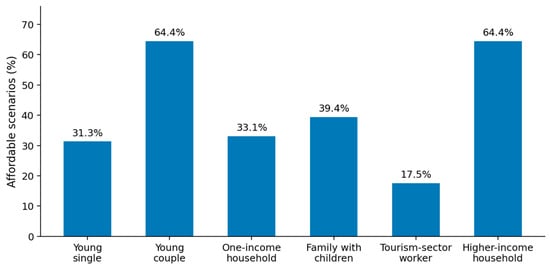
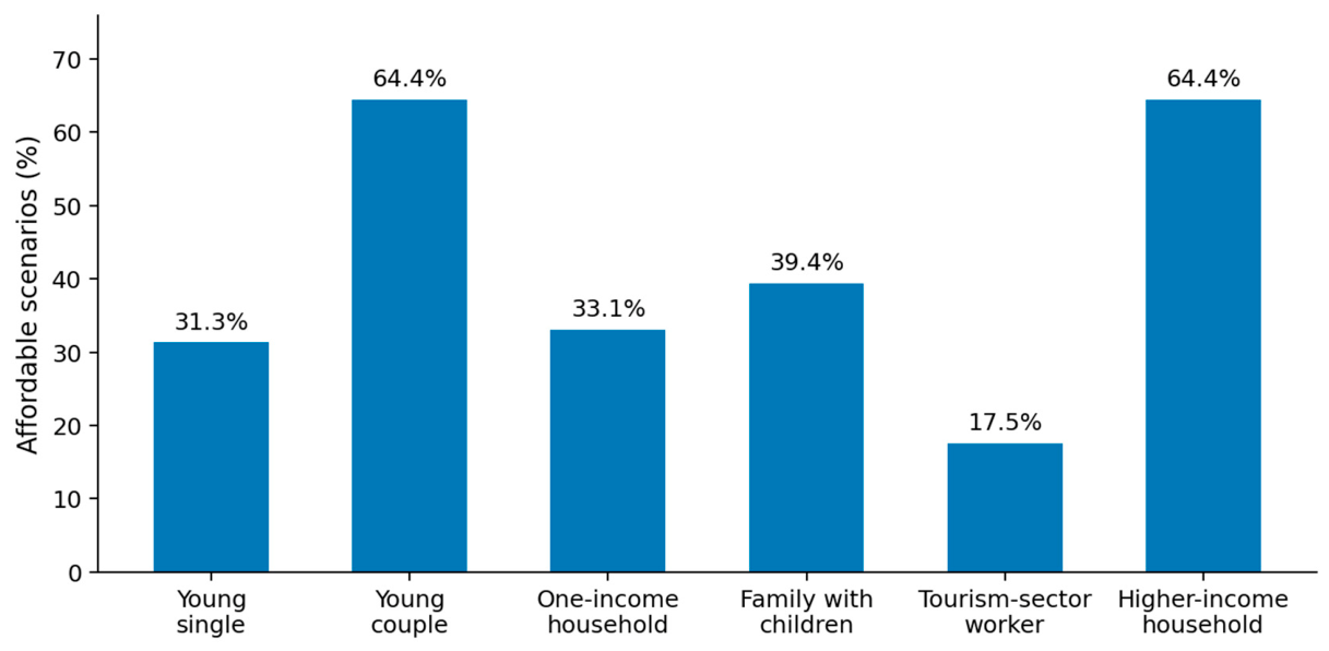
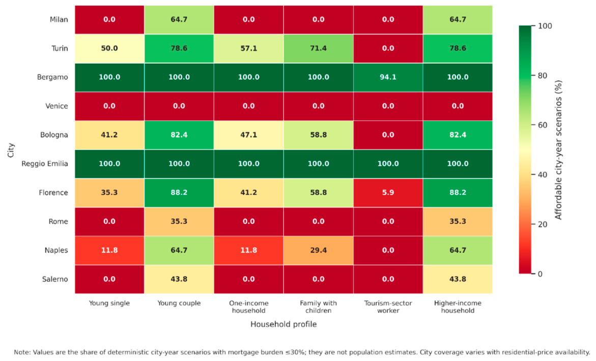
Descriptive comparisons (see Table 3) focus on the available observations in 2008, 2019, 2020 and 2024, representing the start of the study period, the last pre-pandemic year, the tourism collapse and the recovery. City-year values are not imputed solely to complete these reference-year comparisons. Figure 2 reports the affordability classification by city and profile over available years.

Table 3. Descriptive mortgage-financed purchase outcomes by household profile.

Indicator	City-Year N	Young Single	Young Couple	One-Income	Family	Tourism Worker	Higher Income
Mean PTI	160	8.66	6.06	8.49	7.28	11.19	6.06
Mean mortgage burden	160	39.1%	27.4%	38.3%	32.8%	50.5%	27.4%
Mean HOI	160	−30.35	8.75	−27.74	−9.49	−68.45	8.75
Affordable observations (%)	160	31.3	64.4	33.1	39.4	17.5	64.4

Notes: The 160 city-year observations generate 960 deterministic profile scenarios. Percentages are shares of the 160 available scenarios for each profile that satisfy the assumed mortgage-burden threshold, not estimates of the proportion of residents or households able to buy a dwelling. Table 3 indicates that the tourism-sector-worker scenario has the highest mean PTI and mortgage burden and the lowest affordable-scenario share. The young-couple and higher-income profiles have identical outcomes because of their matching dwelling-size-to-income-factor ratios (Table 1).

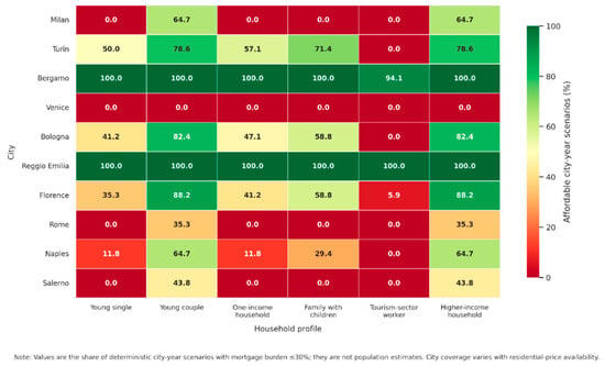
Figure 2. Share of city-year profile scenarios meeting the assumed 30% mortgage-burden threshold. Percentages do not estimate the share of actual households able to purchase a home.

High residential prices do not automatically imply lower simulated purchase affordability because income and mortgage conditions are also taken into account. Tourism intensity is likewise distinguished from formal accommodation capacity. Table 3 summarises the simulated purchase outcomes by household profile.

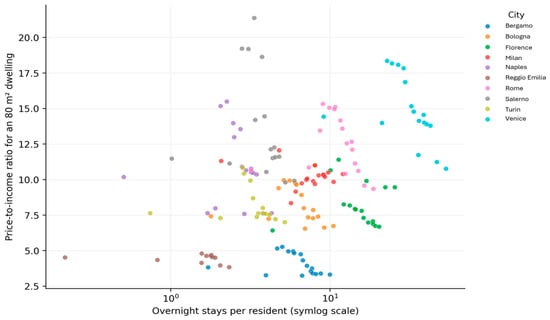
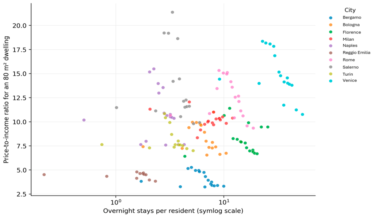
Figure 2 compares simulated purchase classifications across household profiles. Figure 3 illustrates that higher tourism intensity does not uniformly correspond to a higher price-to-income ratio across observed city-years; this association is descriptive rather than causal. At the 35% burden threshold, affordable-scenario shares are 38.75% for young singles, 80.63% for young couples and higher-income households, 39.38% for one-income households, 61.25% for families with children and 25.63% for tourism-sector workers. At 40%, the corresponding shares are 56.88%, 83.75%, 60.00%, 77.50% and 33.75%, with young couples and higher-income households both at 83.75% (Table A5). The tourism-sector-worker scenario remains the most constrained at each threshold. Figure 3 illustrates the descriptive relationship between tourism intensity and the price-to-income ratio across city-year observations.

Figure 3. Tourism intensity and the price-to-income relationship across city-years. Tourism intensity is measured as the number of registered overnight stays per resident; the vertical axis uses the representative 80 m² dwelling PTI (For the city-year econometric models and Figure 3, PTI is calculated as the value of a standardised 80 m² dwelling divided by municipal mean annual taxable income; the household scenarios instead use the profile-specific dwelling sizes and income multipliers reported in Table 1) shown in the plot.

4.1. Econometric Model Results

The first two-way fixed-effects model (see Table 4) estimates log residential price as a function of log municipal income and log tourism intensity. Income remains positive and statistically significant (β = 3.896; clustered SE = 1.548; p = 0.033), whereas tourism intensity is negative but not significant (β = −0.147; SE = 0.224; p = 0.528). The model contains 160 observations, ten city clusters and city and year fixed effects (R² = 0.922).

Table 4. Two-way fixed-effects and exploratory nonlinear estimates.

Variable	Log Price FE	Log PTI FE	Post-COVID FE	Threshold FE
Log municipal income	3.896 ** (1.548)	—	—	—
Log tourism intensity	−0.147 (0.224)	−0.088 (0.204)	−0.235 (0.172)	—
Tourism × Post-2021	—	—	0.100 (0.102)	—
Tourism intensity below 5.94	—	—	—	−0.076 (0.055)
Additional slope above 5.94	—	—	—	0.068 (0.049)
City and year fixed effects	Yes	Yes	Yes	Yes
Observations/cities	160/10	160/10	160/10	160/10
R2	0.922	0.924	0.929	0.928

** indicates statistical significance at the 5% level (p < 0.05). Notes: Parentheses report city-clustered standard errors. The conventional p-values and significance markers are uncertain with only ten city clusters; small-cluster bootstrap inference has not been reported. The breakpoint was selected in sample, and coefficient tests do not account for selection uncertainty.

When log price-to-income is used as the outcome, tourism intensity again has no statistically significant within-city association (β = −0.088; SE = 0.204; p = 0.677; R² = 0.924). The sign should not be interpreted as evidence that tourism improves affordability: the estimate is statistically uncertain, and the available proxy construction provides limited independent within-city variation after fixed effects are included.

The tourism × post-2021 coefficient is positive but statistically uncertain (β = 0.100; SE = 0.102; conventional p = 0.351). An in-sample search selects 5.94 overnight stays per resident as an exploratory breakpoint. The slope below it is −0.076 (conventional p = 0.201), with an additional slope of 0.068 above it (conventional p = 0.203). These unadjusted results do not establish a common threshold or a post-COVID intensification.

4.2. Model Performance

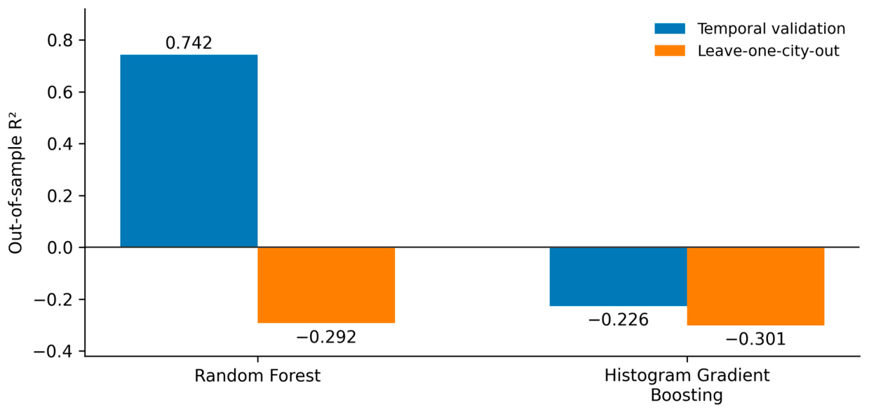
Predictive performance for log PTI was evaluated using tourism intensity, arrival intensity, bed pressure, income, mortgage rates and year. Under leave-one-city-out validation, Random Forest produced R² = −0.292, RMSE = 0.497 and MAE = 0.437; Histogram Gradient Boosting produced R² = −0.301, RMSE = 0.499 and MAE = 0.431. Neither model therefore generalises reliably to an unseen city.

Temporal validation yields a more favourable, although still asymmetric, result. Training on 2008–2019 and testing on 2020–2024, Random Forest achieves R² = 0.742, RMSE = 0.208 and MAE = 0.180. Histogram Gradient Boosting performs poorly (R² = −0.226; RMSE = 0.453; MAE = 0.370). Random Forest therefore predicts observations from later years within the sampled cities but does not generalise well to previously unseen cities.

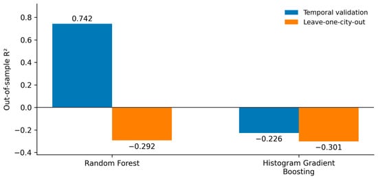
Figure 4 compares out-of-sample R² under temporal and leave-one-city-out validation. Random Forest achieves R² = 0.742 when predicting later observations in represented cities but R² = −0.292 for held-out cities. Histogram Gradient Boosting has negative R² under both temporal (−0.226) and geographic (−0.301) validation (Table 5). Predictive performance within observed cities does not establish transferability to an unseen urban market.

Figure 4. Out-of-sample R² under temporal and leave-one-city-out validation. Negative values indicate predictive performance below the test-set mean benchmark.

Table 5. Predictive performance for log PTI.

Validation/Model	R2	RMSE (log)	MAE (log)
LOCO—Random Forest	−0.292	0.497	0.437
LOCO—Histogram Gradient Boosting	−0.301	0.499	0.431
Train 2008–2019; test 2020–2024—Random Forest	0.742	0.208	0.180
Train 2008–2019; test 2020–2024—Histogram Gradient Boosting	−0.226	0.453	0.370

Figure 5 documents substantial heterogeneity across the ten selected urban markets. No profile-year scenario is classified as affordable in Venice, whereas all available profile-year scenarios satisfy the threshold in Reggio Emilia. Milan, Rome, Naples and Salerno show pronounced differences among assumed profiles; young couples and higher-income households generally perform better because of their assigned dwelling-size-to-income-factor ratios. These are shares of available deterministic scenarios, not shares of actual residents able to purchase a dwelling.

Figure 5. Share of available years in which each household-profile scenario satisfies the assumed 30% mortgage-burden threshold, by city and profile.

5. Discussion

The findings shift attention from average price appreciation to simulated mortgage-financed purchase opportunities. The tourism-sector-worker scenario has a mean PTI of 11.19 and a mean mortgage burden of 50.5%, compared with 6.06 and 27.4% for young couples. These differences depend partly on the stipulated income multipliers and dwelling sizes and are not observed effects on actual household groups.

In the fixed-effects price model, municipal income has a positive coefficient (β = 3.896; conventional p = 0.033), whereas tourism intensity is statistically uncertain both for prices (β = −0.147; p = 0.528) and PTI (β = −0.088; p = 0.677). Studies at different spatial scales and using direct platform measures have reported positive housing-market associations [1,2,4,9,15]. Differences in outcome definition, geography, controls and the reconstructed tourism series may help explain the contrast; the result does not establish an absence of local touristification.

Mikulić et al. [14] examine both tourism and affordability, including the income channel. The scenario comparisons likewise demonstrate why house prices alone cannot characterise purchase burdens across the assumed household profiles. However, these city-year estimates cannot identify individual effects, and tourism coefficients remain exploratory given the reconstructed annual observations.

At the 30% mortgage-burden threshold, 64.4% of young-couple and higher-income scenarios are classified as affordable, compared with 39.4% for families with children, 33.1% for one-income households, 31.3% for young singles and 17.5% for tourism-sector workers.

Differences between profiles illustrate why municipal averages provide only a partial picture of simulated purchase affordability. At the 30% threshold, mean HOI is negative for young singles (−30.35), one-income households (−27.74), families with children (−9.49) and tourism-sector workers (−68.45), while it is 8.75 for young couples and higher-income households (Table 3). These values derive from predefined dwelling sizes and income factors; they are not observed population outcomes.

Research on touristification describes neighbourhood change and place-based exclusion [11,12]. The present city-year scenarios cannot establish whether short-term rentals displaced individual residents, prevented a purchase or caused any particular household to leave.

The exploratory piecewise-linear search yields a breakpoint at 5.94 overnight stays per resident. The estimated slope below it is −0.076, and the additional slope above it is 0.068 (Table 4); neither is statistically supported by the reported conventional tests. The breakpoint was selected on the same sample and must not be interpreted as a verified tourism carrying-capacity threshold. Market-specific responses remain possible, consistent with research on heterogeneous destinations [2,15].

The tourism × post-2021 coefficient is positive (β = 0.100) but statistically uncertain (conventional p = 0.351). The study therefore does not identify a tourism-attributable post-pandemic decline in simulated purchase opportunities. Changing financing conditions and reconstructed tourism series further limit inference for the recovery period.

Random Forest predicts later PTI observations in represented cities (temporal R² = 0.742) but does not transfer reliably to an unseen city (R² = −0.292); Histogram Gradient Boosting has negative R² in both validation designs. As discussed by Mullainathan and Spiess [16], predictive performance answers a different question from econometric inference and cannot establish causal effects.

The city-and-profile comparisons may identify where further local investigation of purchase burdens is warranted. Monitoring visitor accommodation through national registration systems [21] and assessing local regulatory approaches [22] may be helpful alongside measures of housing supply and household income. The reported estimates do not show that reducing tourism would restore affordability; policy suggestions therefore reflect the wider literature rather than an identified causal effect.

The principal limitations concern data quality, observational units and scope. The OMI variable represents selected central or station-area quotation submarkets rather than municipal transaction prices. The sample includes 160 city-year observations for ten cities; only 21 tourism observations are directly observed or recent official anchors, whereas 139 rely on reconstructed proxies. Most reconstructed annual variation follows a common Milan reference series, which may distort within-city relationships. Household profiles are stipulated, rather than observed, and municipal taxable-income proxies do not measure household disposable income, savings or wealth. City-aggregated observations cannot identify neighbourhood displacement or household-level rental affordability. Finally, inference from only ten city clusters and an in-sample breakpoint search is uncertain. Regionally sampled household-budget data and transaction-level dwelling characteristics are unavailable at the necessary resolution for this city-year analysis.

Future research should replace proxy observations with complete municipal and neighbourhood-level series and incorporate platform-level data that distinguish occasional hosts from professional short-term rental operators. Rental prices, housing vacancies, second homes and new housing supply should also be considered alongside purchase prices. Household microdata would allow the simulated profiles to be validated and enable analysis of tenure, wealth and access to mortgage credit.

RQ1 is addressed descriptively through cross-city-and-profile comparisons in Figure 5, which indicate substantial differences among urban markets over their available study years. For RQ2, the fixed-effects models provide no statistically supported tourism association with the selected residential-price proxy (β = −0.147; p = 0.528) or PTI (β = −0.088; p = 0.677). For RQ3, tourism-sector-worker and young-single scenarios have the lowest affordable-scenario shares (17.5% and 31.3%), compared with 64.4% for young-couple and higher-income scenarios. These are not observed household shares or estimates of group-specific causal tourism effects.

6. Conclusions

The study compares deterministic mortgage-financed home-purchase scenarios for six household profiles across ten Italian cities. It finds substantial differences across profiles and urban markets but does not establish a causal tourism effect on housing purchase opportunities. Tourism coefficients, the post-2021 interaction and the exploratory breakpoint are statistically uncertain; model predictions are more reliable for later observations in known cities than for a held-out city. Interpretation is limited by the reconstructed tourism series, selected OMI submarkets, assumed profile resources and lack of rental or household microdata. The comparative framework may help guide more detailed local monitoring, but it cannot determine the share of residents able to buy a home or quantify housing reallocation caused by tourism.

References

- Biagi, B.; Brandano, M.G.; Lambiri, D. Does tourism affect house prices? Evidence from Italy. Growth Change 2015, 46, 501–528. [Google Scholar] [CrossRef] [Scilit]
- Biagi, B.; Brandano, M.G.; Caudill, S.B. Tourism and house prices in Italy: A latent class approach. Tour. Econ. 2016, 22, 964–978. [Google Scholar] [CrossRef] [Scilit]
- Cró, S.; Martins, A.M. Does tourism activity affect house price dynamics? Evidence from tourism-dependent countries. Curr. Issues Tour. 2024, 27, 2780–2798. [Google Scholar] [CrossRef] [Scilit]
- Barron, K.; Kung, E.; Proserpio, D. The effect of home-sharing on house prices and rents: Evidence from Airbnb. Mark. Sci. 2021, 40, 23–47. [Google Scholar] [CrossRef] [Scilit]
- Wachsmuth, D.; Weisler, A. Airbnb and the rent gap: Gentrification through the sharing economy. Environ. Plan. A 2018, 50, 1147–1170. [Google Scholar] [CrossRef] [Scilit]
- Italian National Institute of Statistics (ISTAT). Tourist Flows—Year 2024. Available online: https://www.istat.it/comunicato-stampa/i-flussi-turistici-anno-2024/? (accessed on 28 August 2026).
- Italian National Institute of Statistics (ISTAT). House Prices—Fourth Quarter 2024. Available online: https://www.istat.it/comunicato-stampa/prezzi-delle-abitazioni-dati-provvisori-iv-trimestre-2024/ (accessed on 28 August 2026).
- Biljanovska, N.; Fu, C.; Igan, D. Housing Affordability: A New Data Set; BIS Working Papers No. 1149; Bank for International Settlements: Basel, Switzerland, 2023. [Google Scholar]
- Garcia-López, M.-À.; Jofre-Monseny, J.; Martínez-Mazza, R.; Segú, M. Do short-term rental platforms affect housing markets? Evidence from Airbnb in Barcelona. J. Urban Econ. 2020, 119, 103278. [Google Scholar] [CrossRef] [Scilit]
- Reichle, P.; Fidrmuc, J.; Reck, F. The sharing economy and housing markets in selected European cities. J. Hous. Econ. 2023, 60, 101914. [Google Scholar] [CrossRef] [Scilit]
- Cocola-Gant, A. Place-based displacement: Touristification and neighborhood change. Geoforum 2023, 138, 103665. [Google Scholar] [CrossRef] [Scilit]
- Esposito, A. Tourism-driven displacement in Naples, Italy. Land Use Policy 2023, 134, 106919. [Google Scholar] [CrossRef] [Scilit]
- Office of the United Nations High Commissioner for Human Rights (OHCHR). The Human Right to Adequate Housing. Available online: https://www.ohchr.org/en/special-procedures/sr-housing/human-right-adequate-housing (accessed on 28 August 2026).
- Mikulić, J.; Vizek, M.; Stojčić, N.; Payne, J.E.; Časni, A.Č.; Barbić, T. The effect of tourism activity on housing affordability. Ann. Tour. Res. 2021, 90, 103264. [Google Scholar] [CrossRef] [Scilit]
- Congiu, R.; Pino, F.; Rondi, L. The uneven effect of Airbnb on the housing market: Evidence across and within Italian cities. J. Reg. Sci. 2025, 65, 339–377. [Google Scholar] [CrossRef] [Scilit]
- Mullainathan, S.; Spiess, J. Machine learning: An applied econometric approach. J. Econ. Perspect. 2017, 31, 87–106. [Google Scholar] [CrossRef] [Scilit]
- Agenzia delle Entrate; Osservatorio del Mercato Immobiliare. Banca dati delle Quotazioni Immobiliari. Available online: https://www1.agenziaentrate.gov.it/servizi/Consultazione/ricerca.htm (accessed on 28 August 2026).
- Ministero dell’Economia e delle Finanze. Analisi Statistiche—Dichiarazioni Fiscali: Dati Comunali. Available online: https://www1.finanze.gov.it/finanze/analisi_stat/public/index.php (accessed on 28 August 2026).
- European Central Bank. ECB Data Portal: MFI Interest Rates on Loans to Households for House Purchase—Italy. Available online: https://data.ecb.europa.eu/ (accessed on 28 August 2026).
- Italian National Institute of Statistics (ISTAT). Movimento dei Clienti Negli Esercizi Ricettivi e Capacità degli Esercizi Ricettivi. Available online: https://esploradati.istat.it/ (accessed on 28 August 2026).
- Ministero del Turismo. Banca Dati Strutture Ricettive e Codice Identificativo Nazionale (CIN). Available online: https://www.ministeroturismo.gov.it/banca-dati-strutture-ricettive/ (accessed on 28 August 2026).
- Comune di Firenze. Regolamento per le Locazioni Turistiche Brevi. Available online: https://www.comune.fi.it/ (accessed on 28 August 2026).
Disclaimer/Publisher’s Note: The statements, opinions and data contained in all publications are solely those of the individual author(s) and contributor(s) and not of MDPI and/or the editor(s). MDPI and/or the editor(s) disclaim responsibility for any injury to people or property resulting from any ideas, methods, instructions or products referred to in the content. |
© 2026 by the author. Licensee MDPI, Basel, Switzerland. This article is an open access article distributed under the terms and conditions of the Creative Commons Attribution (CC BY) license.