


Abstract
The classical DiPasquale–Wheaton model has long served as a fundamental framework in real estate economics. However, its implicit assumption of market homogeneity limits its application to the renter-occupied housing market. This paper addresses this structural gap. It introduces a novel conceptual architecture. The model theoretically separates tenants’ pure consumption demand from capital owners’ investment demand. The predictions of the model are confronted with Polish metropolitan data from 2007 to 2025 in a case study of an exogenous demand shock: the influx of refugees from Ukraine in March 2022. The evidence is descriptive and does not claim causal identification. The observed pattern is consistent with the model: a sharp one-off rise in rents was accompanied by a sharp fall in new rental offers, after which nominal rents stabilised, as would be expected if rental demand met an income-based affordability barrier and the market moved from price clearing towards quantity rationing. The model postulates that capitalisation rates are endogenous under conditions of extreme market stress. It also introduces a housing stock leak index alongside a supply allocation parameter. These variables capture structural allocation inefficiencies that may explain why growth in the aggregate housing stock often fails to improve rental housing availability. The ROH model provides an analytical framework for researchers and public policy makers. It indicates that stimulating investment demand without addressing income barriers and physical stock leakage may lead mainly to asset price inflation and deepen housing exclusion. A rigorous test of the income ceiling is left for further research.
1. Introduction
Housing markets represent one of the most complex and socially sensitive segments of modern economies. Fundamental consumption needs intersect here with global investment flows. In recent decades, growing demographic pressure in metropolitan areas, accelerated urbanisation processes, and progressive financialisation [1,2,3] have highlighted the strategic importance of the renter-occupied housing (ROH) market. Abrupt market shocks—such as sudden inflation spikes, migration crises, or construction supply collapses—trigger specific market reactions. These behaviours elude traditional economic description tools. They reveal structural fractures in existing analytical paradigms. The progressive destabilisation of rental housing affordability [4,5] has become a major challenge for public policy makers worldwide. This challenge requires precise theoretical tools. Such tools must clearly explain the shock transmission mechanisms between the real and capital markets.
The widespread use of the classical four-quadrant DiPasquale–Wheaton (DPW) model [6] to analyse the entire housing market remains a fundamental limitation in spatial economics and real estate finance. Although this model provides an unquestionable foundation for integrating the space market with the asset market, it relies on an implicit assumption of participants’ motivational homogeneity. Such an approach is fully justified when analysing the owner-occupied housing (OOH) market. In this market, the same household simultaneously acts as a consumer of housing services and a capital-allocating investor. Directly applying this homogeneous logic to the rental market generates significant cognitive errors. The traditional aggregate approach ignores the dual nature of the rental market. In this market, demand generated by tenants with strictly limited budgets collides with the supply of investors. These investors are guided by financial market logic and expected rates of return rather than the utility of space [7,8].
The literature points to three gaps. First, extensions of the DPW framework have repaired its technical shortcomings, such as the lack of short-run adjustment, search frictions and investor exit dynamics, but have retained a single homogeneous demand curve [9,10,11,12], and the extension that explicitly addresses the OOH/ROH distinction acknowledges that the framework cannot natively distinguish between the objectives of tenants and owners [13]. Models with separate objective functions for investors and households exist outside the four-quadrant tradition [1,7,8,14,15,16,17], but have not been integrated with it. Second, the four-quadrant framework contains no budget constraint on tenant demand, although the rent-burden and eviction literature treats the upper limit of willingness to pay for rent as a binding constraint that generates non-linear adjustments [4,5,18,19,20,21,22,23]. Third, the framework contains no relation between additions to the physical housing stock and the supply of dwellings actually available for long-term rent, although the financialisation, short-term rental and filtration studies show that the two diverge [2,3,24,25,26,27,28,29,30,31,32,33,34,35,36,37,38].
The primary objective of this paper is to address these three gaps. The paper proposes a novel conceptual architecture, the renter-occupied housing model, which separates consumption demand from investment demand. The ROH model allows for non-linear adjustments under conditions of extreme imbalance. Unlike the classical paradigm, the ROH model incorporates the phenomenon of tenant budget rigidity through an upper limit of income-bound rents (RPmax). Beyond this limit, the market is expected to enter a quantity rationing regime. The model also treats the capitalisation rate as endogenous in high-risk environments and introduces a housing stock leak (HSL) index, which captures structural allocation frictions between the expansion of physical housing stock and actual rental offer availability.
Accordingly, the paper addresses three research questions. RQ1: Does separating the objective functions of tenants and owner-investors yield a four-quadrant system with a rent corridor, an endogenous capitalisation rate and a housing stock leak, whose equilibrium exists and is unique? RQ2: Which predictions distinguish this system from the homogeneous DPW model? RQ3: Is the response of the Polish metropolitan rental market to the demand shock of March 2022 consistent with these predictions? RQ1 and RQ2 are addressed analytically in Section 3 and Section 4, and RQ3 descriptively in Section 5. A rigorous test of the predictions, using a measure of the income ceiling that is independent of the data being tested, is left for further research.
To confront the predictions of the model with a situation of severe macroeconomic stress, the study uses a case study of an exogenous demand shock. The Polish metropolitan market from 2007 to 2025 serves as an empirical illustration. Following the influx of war refugees from Ukraine in 2022, this market experienced a large and sudden demand shock. The episode makes it possible to examine whether affordability barriers and transmission lags between rents and transaction prices appear as the model predicts. The same event has been studied with a difference-in-differences design by Głuszak and Trojanek [39], who relate refugee inflows across the five largest Polish cities to changes in rents and prices. The present paper does not seek causal identification: its evidence is descriptive and shows that the observed pattern is consistent with the model, not that the model’s mechanisms are the only possible explanation. The implications for housing policy are therefore presented as conditional on the model.
The structure of the paper is organised as follows. Following this introduction, Section 2 provides a literature review. It critically analyses the evolution of equilibrium models, tenant budget constraints, return endogeneity, and financialisation. Section 3 outlines the theoretical framework and foundational assumptions of the ROH model. It defines the dual nature of the market and the proprietary conceptual apparatus. Section 4 presents the complete four-quadrant formalisation of the described relationships, including the definition, existence, uniqueness and stability of equilibrium (proofs are given in Appendix A). Section 5 confronts the predictions of the model in each of the four quadrants with Polish metropolitan data, using the March 2022 demand shock as a case study. Finally, Section 6 and Section 7 conclude the paper. They provide a broad discussion of the results against the literature, implications for housing policy that are conditional on the model, and main final conclusions.
2. Literature Review
The literature reviewed below falls into four streams, each of which corresponds to a component of the ROH model. Section 2.1 discusses the limitations of the DPW model and the evidence that tenants and owner-investors have different objective functions; it motivates the separation of consumption and investment demand (Section 3.1). Section 2.2 reviews rental affordability limits and household budget constraints, which underlie the rent corridor and the ceiling in Quadrant I. Section 2.3 reviews the determinants of the capitalisation rate and the transmission between rents and transaction prices, which underlie Quadrant II. Section 2.4 reviews the channels through which the growth of the housing stock fails to translate into long-term rental supply (short-term rental conversion, financialisation and the limits of filtration), which underlie the allocation of new supply in Quadrant III and the housing stock leak in Quadrant IV.
2.1. Limitations of the DiPasquale–Wheaton Model and the Foundations of Distinguishing Between OOH and ROH Markets
The classical four-quadrant DiPasquale–Wheaton model from 1992 remains a dominant analytical tool [6]. It integrates the space market with the real estate asset market. In this model, the rent shaped by user demand affects the transaction price of the asset through an exogenous capitalisation rate. This architecture assumes implicit market homogeneity. It treats supply and demand as an aggregate function based on unified participant motivations. This assumption is justified for owner-occupied housing. In this market, a household simultaneously combines the function of a consumer with that of an investor. However, the model fails when applied to the renter-occupied housing market. Consumption and investment demands are separated here between distinct groups of entities. A direct application of the DPW model leads to significant analytical distortions in this case.
The first wave of criticism within the DPW tradition focused on repairing technical flaws. It did not question the homogeneity assumption itself. Colwell [9] identified the lack of a short-term adjustment mechanism. Colwell also pointed out the omission of vacancies and market expectations alongside the exogenous nature of the capitalisation rate. Lisi [10,11] demonstrated the neglect of search and matching frictions in actual transactions. Lisi integrated Mortensen and Pissarides’ theory with the four-quadrant framework. Łaszek [12] extended the DPW model to the commercial real estate market. Łaszek introduced differentiated interest rates and investor exit dynamics. Łaszek showed that the enhanced model loses its character of a mild balancing mechanism and becomes susceptible to shocks. Nevertheless, these extensions preserve the assumption of a homogeneous demand curve. They fail to reconstruct the space market around two separate objective functions.
Direct recognition of the OOH/ROH problem within the DPW tradition comes from Borgersen and Emblem [13]. They reinforced the model with the price-to-rent ratio. They subsequently adjusted it using the loan-to-value (LTV) ratio. The authors state explicitly that they focus on the consumption motive of households rather than the investment motive of landlords. They openly admit that the traditional DPW framework cannot natively distinguish between the objective functions of a tenant and an owner.
A separate strand outside the DPW tradition has developed a formal apparatus for the distinct objective functions of investors and tenants. Turnbull and van der Vlist [7] utilised transactional data from Florida. They defined an owner-occupier’s utility as a function of the property’s consumption value. Conversely, they defined an investor’s utility as a function of expected profit. They empirically demonstrated a systematic price differentiation (known as a rental discount) between investment and owner-occupier transactions on the same asset. Loewenstein and Willen [8] constructed a two-agent model. They introduced separate first-order conditions for each group. They show that treating investors simplistically reduces the price-to-rent ratio to the Gordon growth model. They treat this phenomenon as a special case rather than a general market law. Peng, Yang, and Yang [14] model housing stock allocation as a result of market competition. In this competition, households minimising occupancy costs clash with investors maximising net present value.
Halket, Nesheim, and Oswald [15] estimated a selection model. It shows that ignoring the endogenous allocation of real estate biases the estimates of the price-to-rent relationship. Furthermore, the investor side is not homogeneous. Cook et al. [16] reject the assumption of landlord homogeneity. They document distinct investor archetypes: “flippers”, “milkers”, and “holders” with fundamentally different objective functions. Stirling, Brill, and Purves [17] also warn against treating investors as a homogeneous group. Christophers [1] documents the growing role of institutional investors. They treat single-family homes solely as a financial asset class. These studies confirm that the investment side consists of entities with a decision-making calculus that lacks a counterpart in the consumer-owner problem.
These research streams build on the foundations of classical literature. Poterba [40] established the user cost of capital framework for owner-occupied housing. The framework accounted for taxation, inflation, and financing costs. Himmelberg, Mayer, and Sinai [41] demonstrated the fallacy of conventional price-to-rent indicators without adjusting for the cost of capital. Gallin [42] found that this relationship has predictive power for future prices, but not for rents. This poses a serious empirical challenge to the arbitrage assumption in the DPW model. Henderson and Ioannides [43] were the first to formalise housing tenure choice. They highlighted moral hazard in rental maintenance and limitations in risk diversification. In a later paper [44], they directly separated investment demand from consumption demand for owner-occupied housing. Hung and Tzang [45] decompose housing value into consumption and investment values in a real-options model of homeowners. They cite earlier evidence that tenants tend to view housing as a necessity and buyers as a luxury. Łaszek [46] directly criticised the homogeneity assumption. Łaszek noted that the housing market does not possess a single equilibrium point, but rather a continuum of points. Investors evaluate housing based on its income-generating capacity rather than its ability to satisfy consumption needs. These phenomena necessitate the construction of a new analytical framework. It must natively separate consumption demand from investment demand. This postulate forms the theoretical foundation of the proposed ROH model.
2.2. Rental Affordability Limits and Binding Household Budget Constraints
Identifying the upper bound of willingness to pay for rental housing is a key issue in modern housing economics. The most common operationalisation of this limit is the rent-to-income ratio; the Eurostat definition classes housing costs above 40% of disposable income as overburden [4]. Desmond and Kimbro [18] provide crucial empirical evidence. They demonstrate that eviction resulting from exceeding rent-bearing capacity leads to a drastic deterioration in housing conditions, financial hardship, and health problems.
From a European perspective, Hick, Pomati, and Stephens [4] analyse EU-SILC microdata from 2010 to 2018. They apply a comparative panel analysis based on the Eurostat definition of housing costs exceeding 40% of disposable income. The authors find that affordability problems in the European Union have become more concentrated among market renters. This issue affects them more severely than homeowners and social housing tenants. Dewilde [5] documents a systematic decline in housing affordability for low-income tenants in the private sector across Western Europe. This phenomenon depends on the institutional design of the welfare state. The generosity of housing allowances and the degree of rent regulation play a significant role here. Samarin and Sharma [19] apply principal component analysis and cluster analysis to US data. They demonstrate that the affordability ceiling is determined locally by the labour market’s income structure rather than nationwide rules.
Lens [20] documents the non-linear and asymmetric dimension of rental demand adjustments under shock conditions. In nearly 70% of studied US counties, the number of extremely low-income households per available rental unit increased during the Great Recession (2007–2010). The nationwide affordability gap widened by 17% over three years. In the context of the COVID-19 pandemic, van Vuuren [21] applies hedonics modelling to Dutch transaction data. Van Vuuren demonstrates a measurable drop in willingness to pay for proximity to consumption amenities. This is consistent with a non-linear reallocation of the willingness-to-pay ceiling in response to exogenous shocks. Manville et al. [22] indicate that households unable to pay rent resort to debt substitution strategies. They minimise the rent gap at the expense of accumulating debt in other balance sheet categories. Reina and de la Campa [23] show that this gap was jointly absorbed by tenant arrears and landlords’ balance sheet stress. This finding aligns with the short-term stickiness of contract rents. Coşkun, Apergis, and Coşkun [47] document nonlinear responses of household consumption to wealth, income, and interest rate shocks, which is consistent with such adjustment, although the study does not address rents directly.
Gromis et al. [48] estimated that approximately 2.7 million US households (about 7% of renters) face an eviction filing each year. Büchler, von Ehrlich, and Schöni [49] show that capitalisation rates link rent-income fundamentals with housing supply elasticity. This implies that rental yields cannot permanently decouple from income fundamentals without affecting supply behaviour. The synthesis of these studies leads to a clear conclusion. Contemporary literature treats the upper limit of willingness to pay for rent as a binding constraint. It stems from local income distribution, institutional market structure, and behavioural margins. Exceeding this limit manifests in rent arrears, debt substitution, eviction, and health deterioration. Under market shocks, it triggers non-linear and asymmetric adjustments. These conclusions directly justify the concept of the asymptotic consumption demand barrier RPmax introduced in the ROH model.
2.3. Endogeneity of Capitalisation Rates and Transmission Between Rents and Residential Transaction Prices
The starting point for analysing the relationship between rents and transaction prices is an equilibrium pricing model. In this model, the capitalisation rate breaks down into the risk-free rate, the risk premium, and expected rent growth. Ayuso and Restoy [50] apply this approach to the UK and Spanish markets. They demonstrate that deviations of house prices from fundamentals result from changes in the required risk premium and rental growth expectations rather than market irrationality. Kishor and Morley [51] extend this decomposition to eighteen US metropolitan areas. They find that the non-stationary residual component of the price-to-rent relationship is significant. It reaches particularly high values in metropolitan areas prone to boom–bust cycles. Hendershott and MacGregor [52] find that UK capitalisation rates reflect rational expectations of mean reversion in real cash flows. Investors in the US and Australia did not incorporate such expectations.
Gallin [42] provides empirical evidence on the error correction of prices and rents. Gallin uses quarterly US data from 1970 to 2003 in an error-correction model. When the price-to-rent ratio is high, real prices grow more slowly over the following four years, whereas the ratio has little predictive power for real rents. The adjustment mechanism operates primarily through prices rather than rents. Baltagi and Li [53] study the Singapore market. They find that purchase and rental prices are cointegrated at the local level. The lack of cointegration at the aggregate level indicates the critical importance of data aggregation levels. Ambrose, Eichholtz, and Lindenthal [54] utilise a 355-year dataset from Amsterdam. They document long-term cointegration with persistent deviations from fundamentals. Adjustment to equilibrium can take decades in this case. Hill and Syed [55] apply a hedonic method to 730,000 transactions in Sydney. They demonstrate that quality adjustment reduces the actual price-to-rent ratio by an average of 18%.
Contemporary research treats the capitalisation rate as endogenous. Larriva [56] models capitalisation rates in the multifamily sector as a function of real economic growth relative to inflation. Büchler, von Ehrlich, and Schöni [49] show directly that capitalisation rates are not exogenous. They co-determine with developer decisions and price dynamics, creating a feedback loop that amplifies boom–bust cycles. Baye and Dinger [57] study German microdata. They confirm that rent regulations affect rental investment profitability. Cotton [58] shows that the gap between new tenant rents and the aggregate rent index drives rent inflation. This synthesis leads to a conclusion. When rent growth expectations face affordability barriers or regulations, the valuation channel lowers expected rent growth, raises required returns and risk premiums, and slows error correction. This argument supports the endogeneity of capitalisation rates, providing the theoretical foundation for asset valuation dynamics in the left-hand quadrants of the ROH model.
2.4. Housing Stock Leak: Financialisation, Short-Term Rental Conversion, and New Supply Filtration Limits
The category of housing stock leak denotes a phenomenon where gross stock growth does not translate proportionally into effective long-term rental supply. Although this term has lacked a fully established theoretical definition, it consolidates several important research streams. Fernandez, Hofman, and Aalbers [24] introduce the concept of real estate as a “safe deposit box”. They document that luxury properties in London and New York function as a liquid store of value rather than inhabited housing stock. Atkinson [25] introduces the term necrotecture for newly built super-premium developments in London. They remain empty or underutilised, illustrating the mechanism of cutting off new construction from usable stock. McKenzie and Atkinson [26] document buy-to-leave mechanisms in Kensington and Chelsea. Deliberately leaving purchased homes empty undermines urban planning capacity. Wind, Dewilde, and Doling [27] show that the growth of secondary property ownership withdraws units from the long-term rental pool. This phenomenon concentrates among wealthier households.
The short-term rental conversion channel represents the most direct leakage mechanism. Barron, Kung, and Proserpio [28] demonstrate using US data that total housing supply remains constant. However, available long-term rental space shrinks mechanically as short-term rental supply grows. Koster, van Ommeren, and Volkhausen [29] utilise a quasi-experiment from Los Angeles. They show that short-term rental regulations reduced such listings by 50% and lowered housing prices and rents by about 2%. Pre-regulation Airbnb penetration was associated with a price increase of up to 15% in tourist areas. García-López et al. [30] study data from Barcelona. They demonstrate that districts with high Airbnb penetration experience rent increases ranging from 1.9% to 7%. Wachsmuth and Weisler [31] combine spatial analysis with rent gap theory, estimating units lost from the long-term stock.
The financialisation dimension reveals additional leakage channels through ownership restructuring. Kohl [32] demonstrates a non-linear relationship between mortgage debt and new construction. Once the debt saturation threshold is crossed, additional debt growth correlates with declining construction. Capital flows instead into the privatisation of existing stock and rent extraction. August [2] documents the dynamic growth of REIT market share in Canada. Financialised landlords controlled nearly a fifth of the stock, particularly in provinces with weak rent regulations. Wijburg, Aalbers, and Heeg [3] identify financialisation 2.0. Long-term institutional investment therein enables short-term speculation. Fields [33] documents how automated technologies allow financial firms to scale acquisitions of fragmented single-family rental stock. This is accompanied by underinvestment in maintenance and zero contribution to new supply. Hochstenbach [34] reveals concentrated ownership networks in the Netherlands that restrict stock turnover. Beswick and Penny [35] show how local authorities in London replace public stock with market developments.
Filtration and moving chains literature provides a counterpoint. It indicates that this mechanism operates, albeit with delays. Mast [36] tracks migration chains triggered by new construction in twelve US cities. Nearly 40% of the chain reaches below-median income neighbourhoods by the sixth round of moves. The construction of 100 new market-rate units induces 45 to 70 people to leave low-income neighbourhoods. Asquith, Mast, and Reed [37] show that new buildings lower nearby rents by 5 to 7%. Bratu, Harjunen, and Saarimaa [38] document faster filtration in Helsinki. Every 100 new units generate about 66 available units in low-income areas within a year. The synthesis of these studies leads to a final conclusion. The impact of new supply on rental affordability depends on the allocation channel, filtration time, and ownership structure. Gross stock additions partially leak outside effective long-term rental supply. These phenomena include speculative vacancies, short-term rentals, segmentation, and institutional capital. These frictions indicate that new building stock does not fully convert into available rentals. This motivates incorporating the housing stock leak index and the supply allocation ratio into the ROH model.
In sum, the four streams are complementary but have not been combined in one equilibrium framework. The first identifies the different objectives of tenants and investors, the second an income-bound limit to rents, the third the dependence of the capitalisation rate on risk and the lagged transmission from rents to prices, and the fourth the divergence between the total and the available housing stock. The ROH model integrates these findings in a single four-quadrant system, which is presented in Section 3 and Section 4.
3. Theoretical Framework and Basic Assumptions
3.1. Separating Consumption Demand from Investment Demand: The Dual Nature of the ROH Market
The analytical architecture of the Renter-Occupied Housing (ROH) model serves as a general theoretical tool for developed residential real estate markets. The primary limitation of the classical four-quadrant DiPasquale–Wheaton (DPW) model lies in its assumption of market homogeneity. The DPW model implicitly assumes that the space market and the asset market are driven by actors with unified motivations. This assumption is valid for the owner-occupied housing (OOH) market. A household purchasing a property acts simultaneously as a space consumer and an investor, where consumption and investment utilities are intertwined. However, applying this homogeneous logic to the renter-occupied housing (ROH) market leads to significant analytical distortions.
Figure 1 contrasts the structure of the DPW model (upper panel) with that of the ROH model (lower panel). In the DPW model the real estate market is split into an asset market, linked to the developer market (the construction sector), and a space market, linked to a single space user market in which tenants, owner-occupiers, firms and households are pooled. In the ROH model the dashed vertical line separates the investment side (left) from the consumption side (right). On the left, the rental asset market, whose object of trade is ownership, is linked by a two-way arrow to the investor-owner market, whose participants act on the basis of ownership. On the right, the rental space market, whose object of trade is use or occupancy, is linked by a two-way arrow to the tenant-user market and, through the rental housing stock, to the dwellings available for let. The arrows at the bottom of the panel show how the two sides interact: housing as a capital good generating services (left) is transformed into housing services (right), and the supply of rental housing, which reflects investment demand for rental properties, meets pure consumption demand. Figure 1 is thus a map of the modules and of the actors behind them, whereas Figure 2 shows how the same modules are connected by prices and quantities. The four quadrants of Figure 2 correspond to the modules of Figure 1 as follows: Quadrant I to the rental space market and the tenant-user market, Quadrant II to the rental asset market and the investor-owner market, Quadrant III to the decisions of investor-owners to expand the stock of rental assets through new construction, and Quadrant IV to the rental housing stock available to tenants.
Figure 1.
Conceptual Framework of the ROH Model vs. classic DPW model. Source: own work.
The fundamental assumption of the ROH model is a clear separation of consumption demand from investment demand. The ROH market is a dual system featuring two distinct groups of actors with fundamentally different objective functions. On the one hand, the tenant-user creates the rental space market. Tenants participate exclusively in the space market. Their demand is pure consumption demand, driven by demographics, income levels, housing availability, and preferences. They neither acquire capital assets nor benefit from property appreciation. Their primary economic constraint is the ratio of rental costs to disposable income, which defines their purchasing power. On the other hand, the owner-investor determines the rental asset market. Owners participate primarily in the asset market, treating physical property as a capital allocation vehicle. Their decisions are determined by return on investment, capitalisation rates, maintenance costs, and capital gain expectations. Although they supply space to the user market, their decisions to enter or exit the rental market follow financial market logic rather than residential consumption needs. By formally separating the tenant-user from the owner-investor, the ROH model postulates that equilibrium in the rental market is achieved through continuous tension and interaction between pure consumption constraints—which set the maximum sustainable rent level—and pure investment requirements—which define minimum profitability thresholds.
3.2. Basic Variables of the ROH Model
To maintain analytical consistency with the general DiPasquale–Wheaton architecture, the ROH model operates with a redefined set of market variables. The primary objective of this new categorisation is to separate the consumption sphere from the investment sphere. The two kinds of actors described in Section 3.1 require this reclassification, because the same quantity has a different meaning for a tenant and for an owner. The rent RP and the stock HS belong to the consumption side; the transaction price TP, the capitalisation rate and the assets belong to the investment side; and the parameters r and HSL describe the passage between the two sides (Table 1). The ROH model defines the following baseline variables and structural parameters:
Table 1.
Variables of the ROH model: side of the market, type and unit.
- RP (Rent Price): The equilibrium price in the rental space market, determined by the confrontation of tenants’ pure consumption demand with the available stock. This price reflects the market valuation of the residential service and is constrained by household purchasing power.
- TP (Transaction Price): The unit price of real estate in the asset market, generated by capital owners’ investment demand. It reflects the valuation of a dwelling as an income-generating asset competing with alternative capital placements and the owner-occupied housing market.
- i (Capitalisation Rate): An endogenous discount rate forming a value bridge between the space market and the asset market. In the ROH model, it accounts for specific rental market risks, including regulatory, credit, and liquidity risks arising as rents approach tenants’ income endurance limits.
- HS (Housing Stock): The volume of residential floor space genuinely made available in the long-term rental market. It represents the offer-side utility stock directly utilised by tenant-consumers. Within HS, part of the dwellings is currently let and part is the hidden housing stock (HSH): dwellings of private owners that are not currently let but can enter the rental market within a short period. New rental offers originate in HSH, so the flow of new offers is a short-run indicator of the movement of dwellings from HSH to the let stock.
- HA (Housing Assets): The cumulative, total volume of physical residential stock held by investors and owners. It constitutes the capital foundation of the market, which does not necessarily translate entirely into available rental space.
- C (Construction): The flow of newly built and completed dwellings in a given period, feeding the total residential asset stock.
- HSL (Housing Stock Leak): A proprietary structural parameter determining the degree of allocation inefficiency whereby a portion of the cumulative asset stock is excluded from the long-term rental market (e.g., due to speculative vacancies, conversion to short-term rentals, or legal-administrative barriers), defining the relation . In the formal system of Section 4.5, HSL is endogenous: it rises when rents approach the lower limit RPmin and when financing costs are high.
- r (Supply Allocation Ratio): A parameter determining the fraction of newly built dwellings that flows directly and exclusively into the rental housing market, bypassing the owner-occupied housing market. In Section 4.5, r is endogenous and depends on the profitability of new rental assets relative to financing costs.
- RPmax (Maximum Rent Price Ceiling): A demand parameter determining the maximum budgetary rent rate at which tenants’ disposable income is exhausted, setting an asymptotic resistance threshold for further price increases in the first quadrant of the model.
The presented variables and mechanisms are intended to be general, and their relevance should be examined under severe imbalance conditions. To this end, the proposed framework is confronted with data from a case study of an exogenous demand shock. The Polish rental housing market serves as an empirical illustration. Owing to the recent, abrupt demand and supply shocks, it provides useful material for examining whether the predictions of the model hold under extreme macroeconomic conditions.
4. Architecture and Equilibrium Mechanisms of the ROH Model
The conceptual architecture of the Renter-Occupied Housing (ROH) model relies on the functional and spatial separation of the dual nature of residential real estate markets. The model organises market relationships within a four-quadrant layout divided by two operating axes. The right-hand quadrants (I and IV) constitute the rental space market, representing the space of tenant-users where pure consumption demand is realised. The left-hand quadrants (II and III) form the rental asset market, representing the domain of owner-investors where dwellings are treated as capital goods and decisions rely on pure investment logic. The complete complementation and integration of these subsystems into a single cohesive equilibrium mechanism is illustrated in Figure 2. A key feature of this diagram is its centralised coordinate system, where the origin (zero value) lies at the exact centre of the intersecting axes, and the values of all variables grow outwards centrifugally, serving as the direct analytical reference for the subsequent presentation of empirical results. The meaning of each axis in each quadrant is given in Table 2, and the formal representation of the four relations, together with the definition and properties of equilibrium, is given in Section 4.5.
Figure 2.
Four-quadrant diagram of the Renter-Occupied Housing (ROH) model representing equilibrium mechanisms across space and asset markets. The axes are defined in Table 2 and the curves correspond to Equations (1)–(4) in Section 4.5. Source: own work.
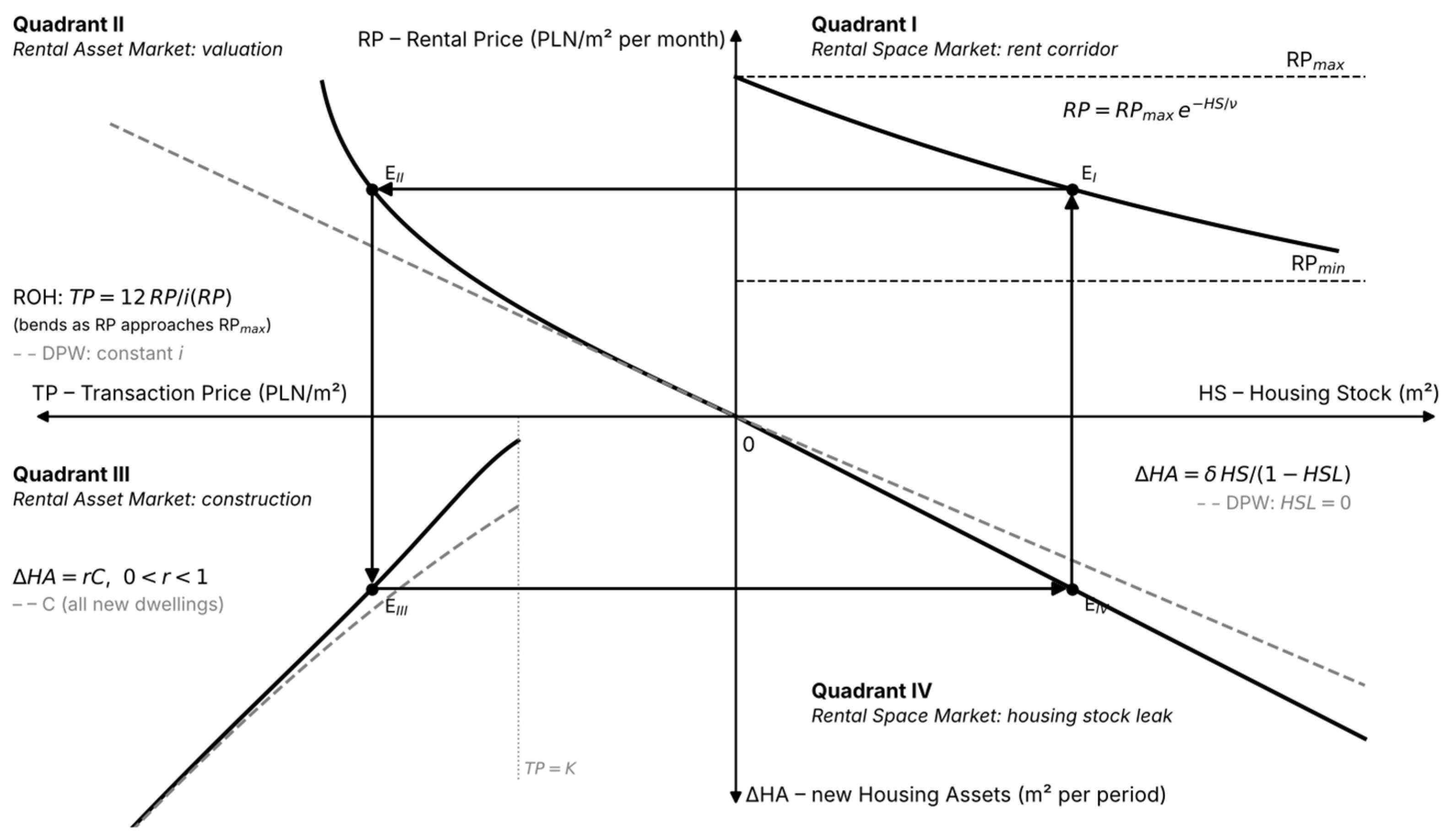
Table 2.
Axes of Figure 2.
4.1. Quadrant I: The Rental Space Market
Quadrant I, located in the upper right section of the model, describes the tenant-user market where rental rates form through the clash of pure consumption demand with the genuinely available rental housing stock. Unlike the classical DiPasquale–Wheaton model, where the space demand curve is continuous and unconstrained, the ROH model introduces the concept of a closed “rent corridor” bounded by two equilibrium thresholds: the upper limit RPmax and the lower limit RPmin.
The upper corridor limit represents the maximum rent level acceptable to consumption demand without triggering abrupt structural adjustments. It is determined by household purchasing power and the alternative cost of servicing mortgage debt in the owner-occupied housing market. When a demand shock pushes rent rates close to RPmax, demand becomes perfectly elastic. Formally, the absolute value of the price elasticity of demand equals and tends to infinity as RP approaches RPmax (Equation (1)). Further rent increases become impossible because, beyond this barrier, tenants are forced into alternatives that are less favourable for them: a transition to OOH, or being pushed into social housing (SOH) or overcrowded dwellings. Rental rates thus encounter a rigid income “ceiling”.
Conversely, the lower corridor limit RPmin establishes the minimum profitability threshold accepted by owner-investors. It covers fixed property maintenance costs, depreciation, transaction costs, and the risk premium against non-payment or vacancy. If a drop in demand forces rents toward RPmin, owners stop offering properties on the pure consumption market. Rather than accepting rates below the profitability threshold, investors choose to withhold properties from the rental market and generate speculative vacancies or liquidate the asset by transferring it to the OOH market.
In formal-functional terms, the mechanism of Quadrant I relies on the collision between the genuinely available stock volume and the pure consumption demand function. The equilibrium point is the rent rate RP where effective demand balances the existing stock HS, subject to the condition that this solution must lie within the open interval (RPmin, RPmax). If an analytically derived rent exceeds RPmax, demand collapses through household allocation to alternative markets, flattening the effective demand curve into a horizontal line. The resulting RP rate serves as an output variable (value input) transmitted via a horizontal relationship vector straight into the upper-left quadrant (Quadrant II), determining the basis for asset capitalisation.
4.2. Quadrant II: The Rental Asset Market (Valuation)
Quadrant II, situated in the upper-left side of the model, shifts the analysis to the owner-investor market. It describes the residential asset valuation mechanism, serving as a value bridge between the rental income stream (RP) and the capital market. The basic valuation relationship takes the form , but in the ROH model, the capitalisation rate (i) ceases to be an exogenous variable imposed exclusively by macroeconomic financial market returns.
The capitalisation rate in the ROH model becomes endogenous and links directly to conditions within the rental asset market. As the rent rate RP approaches RPmax, investors discount higher risks of being unable to raise rates further, rising tenant credit risk, and extended vacancy periods. This increases the rental risk premium, which raises the capitalisation rate i and mitigates further transaction price growth. Additionally, asset valuation on the left side of the model faces continuous pressure from inter-system competition for the exact same physical housing stock between investment demand (for rental purposes) and household consumption demand purchasing dwellings for personal occupancy.
The analytical mechanism of Quadrant II converts the rental income stream transmitted from Quadrant I into asset capital value using a capitalisation ray corresponding to the equation . The key functional relationship of this quadrant is the change in the slope angle of the capitalisation ray depending on the risk level determined in Quadrant I. As RP approaches the upper limit RPmax, it triggers an endogenous increase in rate i, which graphically corresponds to a deflection of the ray and a flattening of the transaction price response TP to rent increases. The resulting transaction price serves as an output signal (Quadrant II output), projected downward via a vertical transmission vector to Quadrant III, triggering an investment impulse on the construction supply side.
4.3. Quadrant III: The Rental Asset Market (Construction for Rent)
Quadrant III, placed in the lower-left side of the model, continues the owner-investor market logic and describes the creation of new construction supply. The asset transaction price level formed in Quadrant II determines the profitability of new development and investment projects, initiating building activity. In the ROH model, however, new supply does not flow entirely into the rental market, distinguishing it from the aggregate treatment in the DiPasquale–Wheaton model.
Due to volume competition with the owner-occupied housing market, the ROH model introduces parameter r, defining the fraction of new supply directed straight and exclusively to the rental asset stock. The r index depends on the institutional structure of the market (e.g., the share of Build-to-Rent institutional investors) and the relative rental yield compared to the margin from selling dwellings on the owner-occupied (OOH) market. Consequently, the elasticity of new rental asset supply is structurally lower than the overall elasticity of the construction market, and transaction price growth only partially translates into an actual expansion of the asset base for the rental market.
Because HA is a stock and C is a flow, the relation between them is one of accumulation, not an identity. New rental assets are a flow, , and the stock evolves as , where is the depreciation rate. In the diagram the lower vertical axis therefore measures the flow , and in a stationary equilibrium (Table 2).
4.4. Quadrant IV: The Rental Space Market (Housing Stock Leak)
Quadrant IV, located in the lower-right section of the model, closes the entire system by returning to the tenant-user market. It describes the mechanism transforming the cumulative volume of residential assets (HA) into genuinely available rental housing stock (HS). Instead of the traditional assumption of simple, linear physical depreciation, the ROH model introduces the Housing Stock Leak (HSL) index.
The HSL mechanism operationalises the phenomenon where physically existing housing assets are not fully accessible to pure consumption demand. Stock leakage includes structural and frictional vacancies, the conversion of long-term rental units to short-term rentals, loss of capital value and technical degradation of dwellings below acceptance thresholds, or owners withdrawing properties in response to unfavourable regulations. Consequently, the genuinely available rental stock equals . Stock leakage rigidifies supply on the right side of the model, directly driving a resurgence of rent pressure in Quadrant I and closing the loop of market dynamics.
4.5. Formal Representation, Equilibrium and Comparative Statics
The four quadrants are represented by four relations with the minimum number of parameters needed to express the mechanisms described above. The relations are one admissible parametrisation, not the only one: any monotone functions with the same properties lead to the same qualitative results. Stocks are measured in m2, RP in PLN/m2 per month and TP in PLN/m2, and is the logistic function (Table 1). The relations follow the sequence of transmission in Figure 2: the stock of assets determines the available stock (Quadrant IV), the available stock and demand determine the rent (Quadrant I), the rent determines the transaction price (Quadrant II), and the transaction price determines new rental assets (Quadrant III), which add to the stock of assets.
Equation (1) describes demand in Quadrant I. Rent falls from the ceiling RPmax as the available stock grows relative to the demand scale , so that as . The absolute value of the price elasticity of demand is , which tends to infinity as : demand is perfectly elastic at the ceiling. The lower limit RPmin does not enter Equation (1); owners respond to rents approaching RPmin by withdrawing dwellings, which is captured by HSL in Equation (4c).
Equation (2a,b) describe Quadrant II. The capitalisation rate equals the base rate ib, determined by financial markets, plus a rental risk premium that rises more than proportionally as the rent approaches the ceiling. For the valuation ray is the constant-rate ray of the DPW model.
Equation (3a–c) describe Quadrant III. Completions react to the transaction price relative to the cost level K, and the fraction r of completions that becomes rental assets depends on the relative profitability of rental assets and on financing costs.
Equation (4a–c) describe Quadrant IV. The leak HSL rises as the rent falls towards the profitability threshold and as financing costs rise. The model nests the DPW model for , and together with a linear demand curve, which is obtained from Equation (1) in the limit with fixed. In that case the system collapses to a single homogeneous demand, a constant capitalisation rate and full transmission of new construction into the available stock.
Equilibrium. A stationary equilibrium is a vector that satisfies Equations (1)–(4) with , i.e., . Substituting Equations (2)–(4) shows that the stationary available stock is a function of the rent alone, , so that the equilibrium rent is a fixed point of . The four-quadrant representation is meaningful in the following sense: the loop of Figure 2 closes at a point E at which the rent implied by demand for the stock, the transaction price implied by the rent, the new assets implied by the price and the stock implied by the assets are mutually consistent. Three propositions describe when such a point exists, when it is unique and when it is stable; the proofs are given in Appendix A.
Proposition 1 (existence).
If , a stationary equilibrium with exists. Otherwise the stock exceeds what demand absorbs at the floor, and (under Proposition 2) the rent settles at RPmin with unlet surplus stock.
Proposition 2 (uniqueness).
The equilibrium is unique if is non-decreasing in RP. A sufficient condition is , together with : a higher rent raises the transaction price, hence completions and the share allocated to rental, and lowers the leak.
Proposition 3 (stability).
Let denote new rental assets implied by the stock HA through Quadrants IV, I, II and III. Under the conditions of Proposition 2, and the stock follows . The equilibrium is locally stable if and converges monotonically if . Delivery lags between the transaction price and completions add dynamics of higher order; cyclical behaviour is then possible, but it is not analysed here.
Table 3 gives the comparative statics of the stationary equilibrium. The sign of the response of RP and HS to most parameters follows from the position of the fixed point (Appendix A); the response of TP combines the movement of RP and of i and is determined numerically for an illustrative calibration (Appendix A.5), as marked by an asterisk.
Table 3.
Comparative statics of the stationary equilibrium: direction of change in the equilibrium value after an increase in the parameter.
The signs show the main logic of the model. An increase in the number of tenants or in incomes raises the rent and the stock, because higher rents induce more construction and a smaller leak. An increase in the cost of capital or in the leak lowers the available stock and raises the rent. An increase in the base capitalisation rate lowers the transaction price and construction and, through a smaller stock, raises the rent.
Predictions that distinguish the ROH model from the DPW model. Three predictions follow from Equations (1)–(4) and differ from those of the DPW model. First, the elasticity of the transaction price with respect to the rent is , which is below one and falls as RP approaches RPmax, whereas the DPW model with a constant capitalisation rate implies . Second, the response of the rent to a demand shock, , where and is the elasticity of the stationary stock with respect to the rent, tends to zero as the rent approaches the ceiling, whereas in the DPW model the response is bounded away from zero. Third, new construction raises the available stock only by the fraction , whereas in the DPW model the fraction is one. Section 5 confronts the first two predictions with the data; r and HSL are not observed in the available series, so the third prediction is not tested.
5. Confronting the Model Predictions with Polish Metropolitan Data
This section confronts the predictions of Section 4.5 with Polish metropolitan data. The aim is limited. The evidence is descriptive: it rests on a single event, has no control group and does not identify causal effects, so it can show that the observed patterns are consistent with the predictions, not that the mechanisms of the ROH model are the only possible explanation. The same event was studied with a difference-in-differences design by Głuszak and Trojanek [39].
Three features of the data matter for interpretation. First, the stock HS is not observed; the available series counts new rental offers, which is a flow originating in the hidden housing stock HSH and serves as an indicator of the short-run availability of dwellings. Second, the capitalisation rate is not observed independently: the gross rate is a definitional ratio of the rent to the price, not an independent measure of the capitalisation rate, so its movements describe the relative movement of rents and prices. Third, the ceiling RPmax is not measured: no series of tenants’ incomes is used, and no parameter of any trend line fitted to the rent series is interpreted as RPmax. A rigorous test of the income ceiling with an independent measure of the ceiling is left for further research.
The data cover Warsaw and the aggregates of the five and ten largest cities: monthly asking rents and new offers for 2021–2025 (60 observations; Otodom Analytics), quarterly transaction prices, rents and completions for 2007–2025 (NBP and Statistics Poland), and annual housing stock for 2009–2025 (Statistics Poland). The first prediction of Section 4.5 (the elasticity of the price with respect to the rent) is examined in Section 5.2 and the second (the weakening response of rents near the ceiling) in Section 5.1. Quadrants III and IV are discussed qualitatively, because r and HSL are not observed in the available series. Regressions use log differences, to avoid spurious relationships between trending series, and Newey–West standard errors (3 lags for monthly and 4 lags for quarterly data). Augmented Dickey–Fuller and KPSS tests (not reported) show that the logarithms of monthly rents and offers are persistent in levels (the ADF test does not reject a unit root) and stationary in first differences (ADF p < 0.001; KPSS does not reject at the 5% level), so the monthly regressions are not exposed to spurious regression. The four-quarter log changes in quarterly prices are not stationary (ADF p = 0.42–0.85; KPSS p ≤ 0.01), so the estimates of Section 5.2 are descriptive.
5.1. Rents and New Offers Around the March 2022 Demand Shock (Quadrant I)
The monthly series cover January 2021 to December 2025: 14 observations before the shock (until February 2022) and 46 from March 2022. Rents are asking rents in PLN/m2. The second variable is the number of new offers, in thousands, an indicator of the flow of dwellings from HSH into the let stock (Section 3.2). Equation (1) implies that, away from the ceiling, a larger availability of dwellings lowers the rent, and that the elasticity of the rent with respect to HS, equal to , tends to zero as the rent approaches RPmax. The second prediction of Section 4.5 is the corresponding weakening of the response of rents to demand shocks.
Figure 3 plots rents against new offers. The plot is a time path, not a demand curve: each point is a month, and the two phases (before March 2022 and from March 2022) are fitted with quadratic trend lines for description only. No parameter of the trend lines is interpreted as RPmax.
Figure 3.
Monthly asking rents (RP, PLN/m2) and new rental offers (thousands; an indicator of the flow of dwellings from HSH) in Warsaw, the five and the ten largest cities, January 2021 to December 2025. Each point is a month; the lines are quadratic trend lines fitted separately for the phases before March 2022 and from March 2022 and are descriptive only. Source: own calculations based on Otodom Analytics.
Before the shock, rents and offers are strongly and negatively related (correlation −0.98 in Warsaw, −0.92 in the five cities and −0.68 in the ten cities), as Equation (1) implies. From March 2022 the correlation is positive (0.74, 0.54 and 0.48): rents stabilise at a higher level while offers recover. This is the pattern of a shift followed by stabilisation, not of movement along a single curve (Table 4). These are correlations of levels in short samples of trending series; they describe the pattern but do not test it, which is why the tests of Table 5 use log differences. The shock appears as a one-off adjustment. In Warsaw the rent rose from 64.73 to 74.62 PLN/m2 within one month (14 log points) while new offers fell from 2.38 to 1.06 thousand (by 56%). In the five cities the rent rose from 49.69 to 58.44 PLN/m2 and offers fell from 2.84 to 1.05 thousand (by 63%); in the ten cities the rent rose from 40.52 to 45.80 PLN/m2 and offers fell from 1.33 to 0.68 thousand (by 49%). The monthly rent changes of 12–16 log points compare with standard deviations of monthly changes of 0.7–1.5 log points before the shock. After allowing for a pre-shock trend, the level shift in the log rent is 0.27 in Warsaw (about 31%), 0.37 in the five cities (44%) and 0.21 in the ten cities (23%) (Table 5). After the shock, nominal rents stabilise. Between 2023 and 2025 they grew by 1.0% per year on average in Warsaw and in the five cities, and by 3.3% in the ten cities, although new offers returned to their pre-shock range (in Warsaw, 2.33–4.29 thousand per month in 2023–2025, compared with 2.05–4.46 thousand before the shock).
Table 4.
Rents and new offers by phase: correlation and fit of the trend lines in Figure 3.
Table 5.
Level shift in rents at March 2022, later rent growth and the response of monthly rent changes to monthly changes in new offers.
The second prediction can be examined by comparing the response of monthly rent changes to monthly changes in new offers before and after the shock (Table 5). Before the shock the response is negative and precisely estimated in all three markets (−0.07 in Warsaw, −0.04 in the five cities and −0.01 in the ten cities). After the shock it is weaker in all three: −0.04 in Warsaw, and close to zero and insignificant in the five cities (−0.003) and in the ten cities (−0.005). The difference between the phases is statistically significant in Warsaw, borderline in the five cities and insignificant in the ten cities. The pattern is consistent with the prediction: after a rise in rents of 23–44%, the rents remain on a high plateau, and their response to the availability of dwellings is weaker than before. The data cannot show that the plateau is an income ceiling. At least three other explanations are consistent with it: the end of the refugee inflow, and the return of some of the newcomers, which would reduce demand without any ceiling; a slow adjustment of asking rents; and a supply response, in which dwellings return from HSH to the let stock. Distinguishing between these explanations requires an independent measure of tenants’ income, which is not used in this paper.
5.2. Capitalisation Rates and Valuation Lags (Quadrant II)
Quadrant II predicts that the capitalisation rate rises with RP/RPmax, so that the price responds less than proportionally to the rent: , and the elasticity falls as the rent approaches the ceiling (Section 4.5). The data are quarterly average secondary-market transaction prices and average rents for 2007–2025 (76 quarters; Figure 4). The capitalisation rate is not observed independently. The gross rate is used, which is a definitional ratio of the rent to the price, so the question is whether prices lagged behind rents after the shock.
Figure 4.
Average rents (RP, PLN/m2 per month) and average secondary-market transaction prices (TP, thousand PLN/m2), quarterly, 2007Q1 to 2025Q4, in Warsaw, the five and the ten largest cities. The lines are quadratic trend lines and are descriptive only; the gross capitalisation rate is . Source: own calculations based on NBP BaRN.
In all three markets the gross rate rose after the shock: in Warsaw from 5.3% in 2021Q4 to 6.1% in 2022Q4 and 6.5% in 2023Q4, and in the five and ten cities to 7.5% and 7.3% in 2022Q4 (Table 6). During 2022 rents rose by 26% in Warsaw, 31% in the five cities and 23% in the ten cities, whereas transaction prices rose by about 10% in all three markets. From 2023 the rate declined, to 5.9%, 6.7% and 6.6% in 2025Q4, as prices grew faster than rents (in Warsaw by 18% against 8% between 2023Q4 and 2025Q4). Prices thus lagged behind rents after the shock and caught up later, as the model’s valuation ray implies. This evidence does not separate a rental risk premium from the cost of financing. The reference rate of the NBP was raised in a series of steps from October 2021 to 6.75% in September 2022 [59], so higher interest rates are an obvious alternative explanation for the increase in the gross rate and for the slowdown in price growth. The paper does not control for interest rates and does not claim that the increase in the gross rate reflects a risk premium related to the ceiling.
Table 6.
Gross capitalisation rate, 12 × rent/price (% per year), selected quarters.
Table 7 reports the pass-through of rent changes to prices in four-quarter log differences. The pass-through is statistically indistinguishable from zero in all but one case, before as well as after the shock (the exception is the five cities before 2022, 0.28, with a standard error of 0.11), and it is clearly below one, as the prediction requires. However, this is not specific to the vicinity of the ceiling: it is observed in 2007–2021, when rents were far from any ceiling. The cumulative ratio of price growth to rent growth was 1.26 in Warsaw in 2007–2021 and 0.77 in 2021Q4–2025Q4; in the five cities it was 0.91 and 0.86, and in the ten cities 0.66 and 0.96. The ratio fell after the shock in Warsaw and, marginally, in the five cities, and rose in the ten cities. The data therefore do not provide robust evidence that the elasticity falls as rents approach the ceiling: the post-shock sample has 16 quarters and the standard errors are 0.14–0.29. In addition, the four-quarter log changes in prices are not stationary, so the estimates in Table 7 describe the data and do not test the prediction. The evidence for Quadrant II is limited to a lag of prices behind rents after the shock, which is compatible with the model but also with the response of the capitalisation rate to interest rates.
Table 7.
Pass-through of rent changes to transaction prices.
5.3. New Construction and Its Allocation to Rental Assets (Quadrant III)
Quadrant III predicts that new rental assets are a fraction r < 1 of the completions that respond to the transaction price, (Equation (3c)). The data are quarterly average primary-market transaction prices and the four-quarter moving average of dwellings completed for sale or rent, 2009–2025 (Figure 5). The completions series is not split between ownership and rental, so r is not observed and the prediction r < 1 is not tested. The series can only show whether completions are related to prices.
Figure 5.
Average primary-market transaction prices (TP, PLN/m2) and the four-quarter moving average of completed dwellings (C, thousands), quarterly, 2009Q4 to 2025Q4, in Warsaw, the five and the ten largest cities. The lines are quadratic trend lines and are descriptive only. Completions are not split between ownership and rental, so r is not observed. Source: own calculations based on NBP BaRN and Statistics Poland.
Completions and prices are positively related in levels: the correlation of the logarithms is 0.80 in the ten cities, 0.66 in the five cities and 0.31 in Warsaw. The correlation does not rise when prices are lagged by two to eight quarters (for example, in the ten cities it falls from 0.80 to 0.69 at eight quarters), so the data do not show the lagged response of completions to prices that is assumed in Section 4.3. These are correlations of trending series, and no conclusion about the elasticity of supply should be drawn from them. The series therefore offers no test of Quadrant III; it only shows that completions and prices move together in the metropolitan markets, in a stronger way in the ten and five cities than in Warsaw.
5.4. Housing Stock and Available Offers (Quadrant IV)
Quadrant IV predicts that the stock available to tenants is a fraction of the housing assets, , and that the leak HSL varies with the rent and financing costs (Equation (4)). The data are annual housing stock and completions for 2009–2025 (Statistics Poland; Figure 6) and the monthly number of new offers used in Section 5.1. Neither HS nor HSL is observed, so this section only places the available series in relation to the model.
Figure 6.
Housing stock (million dwellings, all tenures; horizontal axis) and annual completions (thousand dwellings, an upper bound for the flow ; vertical axis), 2009–2025, in Warsaw, the five and the ten largest cities. The lines are quadratic trend lines and are descriptive only. Neither HS nor HSL is observed. Source: own calculations based on Statistics Poland.
The recorded housing stock grew between 2009 and 2025 from 0.819 to 1.112 million dwellings in Warsaw (36%), from 1.144 to 1.638 million in the five cities (43%) and from 1.197 to 1.482 million in the ten cities (24%). New offers, the only series related to the availability of dwellings, averaged 2.9 thousand per month in Warsaw, 3.8 thousand in the five cities and 1.4 thousand in the ten cities in 2021–2025, that is, about 0.1–0.3% of the stock per month, and they were volatile, as in the March 2022 episode. This is consistent with the view that the stock available to tenants is a small and variable part of the stock, but it does not measure HSL: offers are a flow from HSH and the stock is not observed. The two statistical series are also not reconciled. Cumulative completions reported for 2010–2025 are about twice the increase in the recorded stock (577 against 293 thousand in Warsaw, 1014 against 494 thousand in the five cities and 504 against 284 thousand in the ten cities). The difference reflects differences in coverage and definitions that are not documented in the dataset, and it should not be interpreted as the leak. Estimating HSL and r requires data that separate rental from owner-occupied dwellings and the let stock from vacant dwellings; this is left for further research.
6. Discussion and Implications for Housing Policy
6.1. Synthesis of Results and Confrontation with Literature
The paper proposes that the renter-occupied housing market is a dual system in which tenants’ consumption demand, bounded by income, meets owner-investors’ decisions governed by returns. It shows that this separation can be formalised in a four-quadrant system with a rent corridor, an endogenous capitalisation rate and a housing stock leak, and that the equilibrium of the system exists and, under stated conditions, is unique and stable (Section 4.5). The formalisation differs from the extensions of the DPW model [9,10,11,12,13], which repair technical shortcomings but retain a homogeneous demand curve, in three respects: demand has an income-bound ceiling, the capitalisation rate depends on the rent relative to the ceiling, and new construction reaches the available stock only through the allocation ratio and the leak. It is consistent with the literature that separates the objective functions of investors and owner-occupiers [1,7,8,14,15,16,17], for example the price differences between investor and owner-occupier purchases of the same asset documented by Turnbull and van der Vlist [7] and the two-agent model of Loewenstein and Willen [8].
Quadrant I formalises the rent burden literature [4,5,18,19,20,21,22,23]. The rent-to-income thresholds and the non-linear responses documented by Dewilde [5], Lens [20] and van Vuuren [21] appear in the model as an upper limit RPmax at which the demand for rental housing is perfectly elastic. In contrast to linear and logarithmic demand specifications, Equation (1) has the ceiling as its intercept. The Polish evidence (Section 5.1) is consistent with a weakening response of rents to the availability of dwellings after the shock of March 2022. It does not identify the ceiling, and it does not exclude alternative explanations, namely the end of the refugee inflow, a slow adjustment of asking rents and a supply response. The difference-in-differences study of the same event by Głuszak and Trojanek [39] is complementary, because it addresses causal identification, which this paper does not.
Quadrant II relates to the literature in which the capitalisation rate depends on the risk premium and on expectations of rent growth [50,51], and in which prices respond to rents with a lag [42,54]. The ROH model adds the dependence of the premium on the rent relative to the ceiling. The Polish data show that prices lagged behind rents after the shock, in line with the literature on transmission lags, but they do not show that the pass-through falls near the ceiling, and the increase in the gross capitalisation rate coincides with the increase in the NBP reference rate (Section 5.2). The endogeneity of the capitalisation rate is therefore an assumption of the model, supported by the literature [49], with which the Polish data are consistent but which they do not test.
Quadrants III and IV relate to the literature on leakage through short-term rental conversion [28,29,30,31], financialisation [2,3,24,32] and the limits of filtration [36,37,38]. The allocation ratio r and the leak HSL summarise these channels in two parameters. The literature shows both that the growth of the gross stock does not translate proportionally into long-term rental supply and that filtration operates, albeit with delays [36,37,38]. The ROH model is consistent with both, because the leak is allowed to vary. The Polish data do not measure r or HSL (Section 5.3 and Section 5.4), so the contribution of the paper in these quadrants is the formal structure, not estimates.
6.2. General Implications for Housing Policy
The implications below are conditional on the model and on the descriptive evidence of Section 5. They are hypotheses for the design of policy, not tested conclusions. They are organised by the channel of the model through which an instrument acts, because the four channels respond to different instruments and the model predicts different effects for each.
Tenants’ income and the rent ceiling (Quadrant I). Housing allowances and other support for tenants’ incomes act on the ceiling RPmax. They raise the rent that tenants can afford, but in Equation (1) a higher ceiling also raises the rent at a given stock. If the available stock does not grow, part of the gain may therefore be capitalised in higher rents. The incidence of such support between tenants and owners is not known for Poland. Its effect should be assessed with the rent-to-income ratio RP/HI, where HI denotes average wages, a proxy for tenants’ income.
Cost of capital and valuation (Quadrant II). Preferential mortgages, investor tax reliefs and interest rate subsidies change the investors’ cost of capital or the base capitalisation rate (Table 3, ib and rf). They move transaction prices and construction but do not move the income-bound ceiling, so they affect rents only indirectly, through the stock. A measure aimed at affordability should therefore be evaluated for its effect on the rent corridor, and not only on prices and construction.
Allocation of new construction (Quadrant III). New construction adds to the stock of assets. Instruments that raise the allocation ratio r, such as support conditional on long-term letting or the development of institutional rental, raise ΔHA for a given volume of completions. The tenure split of completions is not observed, so neither r nor the fiscal cost of such instruments can be assessed.
Housing stock leak (Quadrant IV). Only the fraction of completions reaches tenants. Reducing the leak HSL raises the available stock without construction: by limiting the conversion of long-term lettings to short-term rentals, whose effects on rents and prices are documented in the literature [28,29,30], by making the legal framework for long-term lettings more predictable, which reduces owners’ risk, or by incentives to let vacant dwellings. The literature also shows that regulation may change owners’ investment incentives [57], which in the model would appear as a change in HSL or r, so the net effect of a regulatory measure is not determined a priori. The size of HSL in Poland is not estimated, and the compliance and administrative costs of these instruments have not been assessed.
The channels also interact. Because of the capitalisation of income support described above, support for tenants’ incomes should be assessed together with measures that raise the available stock, and not in isolation.
The model also suggests a monitoring system for affordability stress based on the ratio of the rent to the income-based ceiling. Because the ceiling is not observed and may differ between cities, the indicator is RP/HI, and the thresholds are percentiles of the city’s own history, set before the data are analysed. The system has two levels (Table 8). The first level is a rent-to-income ratio that is persistently high. The second level combines this with a sharp fall in new offers, the signal observed in March 2022, when new offers fell by 49–63% within a month (Section 5.1). The thresholds in Table 8 are illustrative; they have not been calibrated or validated, and their false-alarm rate is unknown. Before use, they should be tested on historical data for several cities.
Table 8.
Illustrative early-warning system for affordability stress.
Moving from these hypotheses to recommendations requires three kinds of data: a split of completions and of the stock between rental and owner-occupied dwellings, a split of the stock between let and vacant dwellings, and an independent measure of tenants’ income.
6.3. Study Limitations and Directions for Future Research
The study has several limitations that determine how its results should be read. First, the confrontation with data is descriptive: it rests on one event, has no control group and does not identify causal effects. Second, the stock HS is not observed, and the number of new offers, a flow originating in HSH, is used as an indicator of availability. Third, the capitalisation rate is measured as the definitional ratio 12 RP/TP and cannot be separated from the cost of financing, so the Polish data cannot be used to test the dependence of the capitalisation rate on the rent relative to the ceiling. Fourth, no measure of tenants’ income is used and the ceiling RPmax is not measured, so the existence of an income ceiling is not tested; the stabilisation of nominal rents after 2022 is consistent with a ceiling but also with other explanations. Fifth, r and HSL are not identified, because the available series do not separate rental from owner-occupied dwellings or the let stock from vacant dwellings, and the series of completions and of the housing stock are not reconciled. Sixth, the equations of Section 4.5 are one admissible parametrisation, and the calibration in Appendix A.5 is illustrative and not estimated. Finally, the institutional specificity of the Polish market, with a high share of private ownership and a small institutional rental market, calls for caution when the results are transferred to markets with different structures.
Directions for future research follow from these limitations. The most important is a rigorous test of the income ceiling and of the rent corridor, with a measure of the ceiling that is independent of the series being tested, pre-specified predictions and a design that addresses the common shocks to rents and prices; it is planned as a separate study. Further directions are the estimation of HSL and r with data that separate rental, owner-occupied and vacant dwellings, the analysis of delivery lags between prices and completions, and panel estimation of the model for several countries.
7. Conclusions
This paper addresses a limitation of the four-quadrant DiPasquale–Wheaton model, which assumes that the motivations of the users and owners of space are homogeneous. The ROH model separates the consumption demand of tenants, bounded by income, from the investment demand of owners, driven by returns on capital. It expresses this separation in a four-quadrant system with a rent corridor, an endogenous capitalisation rate, an allocation ratio of new supply and a housing stock leak. The stationary equilibrium of the system exists, and it is unique and stable under the conditions stated in Propositions 1–3. Three predictions distinguish the model from the DPW model: the elasticity of the price with respect to the rent is below one and falls near the ceiling, the response of rents to demand shocks vanishes near the ceiling, and new construction reaches the available stock only in part.
The predictions were confronted with Polish metropolitan data for 2007–2025, using the demand shock of March 2022 as a case study. The evidence is descriptive. After the shock, rents rose by 23–44% beyond the pre-shock trend while new offers fell by 49–63% in a month; from 2023, nominal rents grew by 1.0–3.3% a year although offers returned to their earlier range, and the response of rents to offers weakened in Warsaw and in the five cities. These results are consistent with the prediction for Quadrant I, but they do not identify an income ceiling. Prices lagged behind rents after the shock, and the gross capitalisation rate in Warsaw rose from 5.3% to 6.5% in two years and then fell to 5.9%; this is compatible with the model but also with the rise in interest rates, and there is no robust evidence that the pass-through of rents to prices falls near the ceiling. The allocation ratio and the leak are not identified in the available data.
The model has three implications for the analysis of housing policy, which are conditional on the model. The tenant side and the investor side of the rental market respond to different instruments and should be assessed separately. Support for tenants’ incomes may be partly capitalised in rents unless the stock available to tenants increases at the same time, and this stock can be increased by reducing the leak as well as by construction. The rent-to-income ratio, together with a fall in new offers, is a candidate signal for monitoring affordability stress; its thresholds need to be calibrated. A rigorous test of the income ceiling, with an independent measure of the ceiling, is the main task for further research and is planned as a separate study.
Declaration of Generative AI and AI-Assisted Technologies in the Writing Process
During the preparation of this paper, the author used Perplexity Pro in order to assist with the preliminary literature review and identification of key sources. Furthermore, Gemini Pro was used to assist with the graphical abstract generation as well as advanced English language proofreading and stylistic refinement. Claude (Anthropic) supported the analytical work, including formal derivations, numerical checks and descriptive statistics. After using these tools, the author reviewed and edited the content as needed and takes full responsibility for the content of the publication.
Funding
This research received no external funding.
Data Availability Statement
The raw data supporting the conclusions of this article will be made available by the author on request.
Conflicts of Interest
The author declares no conflict of interest.
Appendix A. Formal Results and Proofs
Appendix A.1
Preliminaries. Define , where and is obtained from the stationary condition and Equations (2)–(4). All functions are continuous in RP. From Equation (1), , so that and the absolute value of the elasticity of demand equals .
Appendix A.2
Proof of Proposition 1.
At the ceiling, whenever . At the floor, if and only if , i.e., . As F is continuous, the intermediate value theorem gives a root in . If and F is decreasing (Proposition 2), there is no root in the corridor and the rent is at the floor. □
Appendix A.3
Proof of Proposition 2.
If is non-decreasing, is non-increasing and F is strictly decreasing, so F has at most one root. For the sufficient condition, let . From Equations (2a,b), , which is positive if and only if . Then TP is increasing in , so is increasing by (3a) and is non-decreasing by (3b) for . By (4c) with , is non-increasing in . Hence , a product of non-negative non-decreasing functions, is non-decreasing. If the condition fails near the ceiling, may decline there and multiple equilibria cannot be excluded analytically; the condition is sufficient, not necessary. □
Appendix A.4
Proof of Proposition 3 and comparative statics.
Given the stock HA, the rent solves . Under the conditions of Proposition 2 the right-hand side is decreasing in RP and in HA, so the solution exists, is unique and decreasing in HA. New assets are increasing in RP, hence . The map has . The fixed point is locally stable if , i.e., , which for reduces to ; convergence is monotone if , i.e., . For comparative statics, let be a parameter of . By the implicit function theorem , and under Proposition 2, so the sign of the response of the rent equals the sign of (taking at fixed RP). A parameter that lowers (, , , , ) raises and thus the rent; a parameter that raises () lowers it; an increase in raises . The response of HS follows from (1), , except for and RPmax, where it follows from the monotonicity of and, for RPmax, from the numerical solution. Because does not depend on , differentiating with respect to gives with , which tends to zero as . □
Appendix A.5
Illustrative calibration. The signs marked with an asterisk in Table 3 and the curves of Figure 2 were obtained for the following values, which are chosen for illustration and are not estimates: , , , , , , , , , , , , , (the effect of was evaluated as a joint change of and ). Since , the sufficient condition of Proposition 2 holds on the whole corridor, so that is increasing in throughout. The solution is , , , , and , so that the equilibrium is stable and converges monotonically, and F is strictly decreasing on the corridor. Comparative statics were computed by re-solving the system after an increase of 10–20% in each parameter (or of 0.5 in , ).
References
- Christophers, B. How and Why U.S. Single-Family Housing Became an Investor Asset Class. J. Urban Hist. 2023, 49, 430–449. [Google Scholar] [CrossRef] [Scilit]
- August, M. The financialization of Canadian multi-family rental housing: From trailer to tower. J. Urban Aff. 2020, 42, 975–997. [Google Scholar] [CrossRef] [Scilit]
- Wijburg, G.; Aalbers, M.B.; Heeg, S. The Financialisation of Rental Housing 2.0: Releasing Housing into the Privatised Mainstream of Capital Accumulation. Antipode 2018, 50, 1098–1119. [Google Scholar] [CrossRef] [Scilit]
- Hick, R.; Pomati, M.; Stephens, M. Housing affordability and poverty in Europe: On the deteriorating position of market renters. J. Soc. Policy 2025, 54, 1072–1095. [Google Scholar] [CrossRef] [Scilit]
- Dewilde, C. Explaining the declined affordability of housing for low-income private renters across Western Europe. Urban Stud. 2018, 55, 2618–2639. [Google Scholar] [CrossRef] [Scilit]
- DiPasquale, D.; Wheaton, W.C. The Markets for Real Estate Assets and Space: A Conceptual Framework. Real Estate Econ. 1992, 20, 181–198. [Google Scholar] [CrossRef] [Scilit]
- Turnbull, G.K.; Van Der Vlist, A.J. Bargaining power and segmented markets: Evidence from rental and owner-occupied housing. Real Estate Econ. 2022, 50, 1307–1333. [Google Scholar] [CrossRef] [Scilit]
- Loewenstein, L.; Willen, P. House Prices and Rents in the 21st Century; Social Science Research Network; National Bureau of Economic Research: Cambridge, MA, USA, 2023; Available online: https://www.nber.org/papers/w31013 (accessed on 1 November 2026).
- Colwell, P.F. Tweaking the DiPasquale-Wheaton Model. J. Hous. Econ. 2002, 11, 24–39. [Google Scholar] [CrossRef] [Scilit]
- Lisi, G. Real Estate Macroeconomics and the Four-Quadrant Model: DiPasquale-Wheaton-Colwell Meet Mortensen-Pissarides. J. Real Estate Pract. Educ. 2015, 18, 87–106. [Google Scholar] [CrossRef] [Scilit]
- Lisi, G. Tweaking the DiPasquale–Wheaton–Colwell model. Lett. Spat. Resour. Sci. 2020, 13, 201–208. [Google Scholar] [CrossRef] [Scilit]
- Łaszek, J. The Contemporary DPW Model for the Commercial Real Estate Sector and Its Analytical Capabilities. Real Estate Manag. Valuat. 2025, 33, 87–100. [Google Scholar] [CrossRef] [Scilit]
- Borgersen, T.-A.; Emblem, A.W. Mortgage market induced booms and busts in the housing market in a modified DiPasquale-Wheaton Model. Int. Real Estate Rev. 2022, 25, 281–306. [Google Scholar]
- Peng, C.-W.; Yang, J.T.; Yang, T.T. Determinant of Allocation of Housing Inventory: Competition Between Households and Investors. Int. Real Estate Rev. 2020, 23, 963–991. [Google Scholar]
- Halket, J.; Nesheim, L.; Oswald, F. The Housing Stock, Housing Prices, and User Costs: The Roles of Location, Structure, and Unobserved Quality. Int. Econ. Rev. 2020, 61, 1777–1814. [Google Scholar] [CrossRef] [Scilit]
- Cook, T.M.; Rongerude, J.; Mueller, E.; Kuhlmann, D. Providing Rental Housing: A Systematic Literature Review of Residential Rental Property Owner Decision Making. J. Plan. Lit. 2024, 39, 535–547. [Google Scholar] [CrossRef] [Scilit]
- Stirling, P.; Brill, F.; Purves, A. Conceptualising ‘residential investment’: Separating the inseparable in asset-based economies. Int. J. Hous. Policy 2024, 24, 569–595. [Google Scholar] [CrossRef] [Scilit]
- Desmond, M.; Kimbro, R.T. Eviction’s Fallout: Housing, Hardship, and Health. Soc. Forces 2015, 94, 295–324. [Google Scholar] [CrossRef] [Scilit]
- Samarin, M.; Sharma, M. A typology of U.S. metropolises by rent burden and its major drivers. GeoJournal 2023, 88, 4887–4906. [Google Scholar] [CrossRef] [Scilit]
- Lens, M.C. Extremely low-income households, housing affordability and the Great Recession. Urban Stud. 2018, 55, 1615–1635. [Google Scholar] [CrossRef] [Scilit]
- van Vuuren, A. Is there a diminishing willingness to pay for consumption amenities as a result of the COVID-19 pandemic? Reg. Sci. Urban Econ. 2023, 98, 103858. [Google Scholar] [CrossRef] [Scilit]
- Manville, M.; Monkkonen, P.; Lens, M.C.; Green, R. Renter Nonpayment and Landlord Response: Evidence from COVID-19. Hous. Policy Debate 2023, 33, 1333–1367. [Google Scholar] [CrossRef] [Scilit]
- Reina, V.J.; de la Campa, E.A. Landlords’ rental businesses before and after the COVID-19 pandemic: Evidence from a National Cross-Site Survey. J. Hous. Econ. 2023, 59, 101904. [Google Scholar] [CrossRef] [Scilit]
- Fernandez, R.; Hofman, A.; Aalbers, M.B. London and New York as a safe deposit box for the transnational wealth elite. Environ. Plan. A 2016, 48, 2443–2461. [Google Scholar] [CrossRef] [Scilit]
- Atkinson, R. Necrotecture: Lifeless Dwellings and London’s Super-Rich. Int. J. Urban Reg. Res. 2019, 43, 2–13. [Google Scholar] [CrossRef] [Scilit]
- McKenzie, R.; Atkinson, R. Anchoring capital in place: The grounded impact of international wealth chains on housing markets in London. Urban Stud. 2020, 57, 21–38. [Google Scholar] [CrossRef] [Scilit]
- Wind, B.; Dewilde, C.; Doling, J. Secondary property ownership in Europe: Contributing to asset-based welfare strategies and the ‘really big trade-off’. Int. J. Hous. Policy 2020, 20, 25–52. [Google Scholar] [CrossRef] [Scilit]
- Barron, K.; Kung, E.; Proserpio, D. The Effect of Home-Sharing on House Prices and Rents: Evidence from Airbnb. Mark. Sci. 2021, 40, 23–47. [Google Scholar] [CrossRef] [Scilit]
- Koster, H.R.A.; van Ommeren, J.; Volkhausen, N. Short-term rentals and the housing market: Quasi-experimental evidence from Airbnb in Los Angeles. J. Urban Econ. 2021, 124, 103356. [Google Scholar] [CrossRef] [Scilit]
- Garcia-López, M.-À.; Jofre-Monseny, J.; Martínez-Mazza, R.; Segú, M. Do short-term rental platforms affect housing markets? Evidence from Airbnb in Barcelona. J. Urban Econ. 2020, 119, 103278. [Google Scholar] [CrossRef] [Scilit]
- Wachsmuth, D.; Weisler, A. Airbnb and the rent gap: Gentrification through the sharing economy. Environ. Plan. A 2018, 50, 1147–1170. [Google Scholar] [CrossRef] [Scilit]
- Kohl, S. Too much mortgage debt? The effect of housing financialization on housing supply and residential capital formation. Socio-Econ. Rev. 2021, 19, 413–440. [Google Scholar] [CrossRef] [Scilit]
- Fields, D. Automated landlord: Digital technologies and post-crisis financial accumulation. Environ. Plan. A 2022, 54, 160–181. [Google Scholar] [CrossRef] [Scilit]
- Hochstenbach, C. Networked geographies of private landlordism: Mapping flows of capital accumulation and rent extraction. Hous. Stud. 2023, 39, 2234–2259. [Google Scholar] [CrossRef] [Scilit]
- Beswick, J.; Penny, J. Demolishing the Present to Sell off the Future? The Emergence of ‘Financialized Municipal Entrepreneurialism’ in London. Int. J. Urban Reg. Res. 2018, 42, 612–632. [Google Scholar] [CrossRef] [Scilit]
- Mast, E. JUE Insight: The effect of new market-rate housing construction on the low-income housing market. J. Urban Econ. 2023, 133, 103383. [Google Scholar] [CrossRef] [Scilit]
- Asquith, B.J.; Mast, E.; Reed, D. Local Effects of Large New Apartment Buildings in Low-Income Areas. Rev. Econ. Stat. 2023, 105, 359–375. [Google Scholar] [CrossRef] [Scilit]
- Bratu, C.; Harjunen, O.; Saarimaa, T. JUE Insight: City-wide effects of new housing supply: Evidence from moving chains. J. Urban Econ. 2023, 133, 103528. [Google Scholar] [CrossRef] [Scilit]
- Głuszak, M.; Trojanek, R. War in Ukraine, the refugee crisis, and the Polish housing market. Hous. Stud. 2025, 40, 1043–1065. [Google Scholar] [CrossRef] [Scilit]
- Poterba, J.M. Tax subsidies to owner-occupied housing: An asset-market approach. Q. J. Econ. 1984, 99, 729–752. [Google Scholar] [CrossRef] [Scilit]
- Himmelberg, C.; Mayer, C.; Sinai, T. Assessing High House Prices: Bubbles, Fundamentals and Misperceptions. J. Econ. Perspect. 2005, 19, 67–92. [Google Scholar] [CrossRef] [Scilit]
- Gallin, J. The Long-Run Relationship Between House Prices and Rents. Real Estate Econ. 2008, 36, 635–658. [Google Scholar] [CrossRef] [Scilit]
- Henderson, J.V.; Ioannides, Y.M. A Model of Housing Tenure Choice. Am. Econ. Rev. 1983, 73, 98–113. [Google Scholar]
- Henderson, J.V.; Ioannides, Y.M. Owner occupancy: Investment vs consumption demand. J. Urban Econ. 1987, 21, 228–241. [Google Scholar] [CrossRef] [Scilit]
- Hung, C.-H.; Tzang, S.-W. Consumption and investment values in housing price: A real options approach. Int. J. Strateg. Prop. Manag. 2021, 25, 278–290. [Google Scholar] [CrossRef] [Scilit]
- Łaszek, J. Housing in Consumer’s Theory; MunichPersonal RePEc: Munich, Germany, 2013; Available online: https://ideas.repec.org/p/pra/mprapa/52365.html (accessed on 22 October 2026).
- Coşkun, Y.; Apergis, N.; Coskun, E.A. Nonlinear responses of consumption to wealth, income, and interest rate shocks. Empir. Econ. 2022, 63, 1293–1335. [Google Scholar] [CrossRef] [Scilit]
- Gromis, A.; Fellows, I.; Hendrickson, J.R.; Edmonds, L.; Leung, L.; Porton, A.; Desmond, M. Estimating eviction prevalence across the United States. Proc. Natl. Acad. Sci. USA 2022, 119, e2116169119. [Google Scholar] [CrossRef] [Scilit]
- Büchler, S.; Ehrlich, M.V.; Schöni, O. The amplifying effect of capitalization rates on housing supply. J. Urban Econ. 2021, 126, 103370. [Google Scholar] [CrossRef] [Scilit]
- Ayuso, J.; Restoy, F. House prices and rents: An equilibrium asset pricing approach. J. Empir. Financ. 2006, 13, 371–388. [Google Scholar] [CrossRef] [Scilit]
- Kishor, N.K.; Morley, J. What factors drive the price–rent ratio for the housing market? A modified present-value analysis. J. Econ. Dyn. Control 2015, 58, 235–249. [Google Scholar] [CrossRef] [Scilit]
- Hendershott, P.H.; MacGregor, B.D. Investor Rationality: Evidence from U.K. Property Capitalization Rates. Real Estate Econ. 2005, 33, 299–322. [Google Scholar] [CrossRef] [Scilit]
- Baltagi, B.H.; Li, J. Cointegration of matched home purchases and rental price indexes—Evidence from Singapore. Reg. Sci. Urban Econ. 2015, 55, 80–88. [Google Scholar] [CrossRef] [Scilit]
- Ambrose, B.W.; Eichholtz, P.; Lindenthal, T. House Prices and Fundamentals: 355 Years of Evidence. J. Money Credit Bank. 2013, 45, 477–491. [Google Scholar] [CrossRef] [Scilit]
- Hill, R.J.; Syed, I.A. Hedonic price–rent ratios, user cost, and departures from equilibrium in the housing market. Reg. Sci. Urban Econ. 2016, 56, 60–72. [Google Scholar] [CrossRef] [Scilit]
- Larriva, M. Cap rates as a function of real economic growth. J. Risk Financ. Manag. 2022, 15, 324. [Google Scholar] [CrossRef] [Scilit]
- Baye, V.; Dinger, V. Investment incentives of rent controls and gentrification: Evidence from German micro data. Real Estate Econ. 2024, 52, 843–884. [Google Scholar] [CrossRef] [Scilit]
- Cotton, C.D. Understanding CPI shelter inflation: The importance of the new-tenant/all-tenant rent gap. J. Hous. Econ. 2026, 71, 102117. [Google Scholar] [CrossRef] [Scilit]
- National Bank of Poland (NBP). Press Release from the Meeting of the Monetary Policy Council Held on 7 September 2022. Available online: https://nbp.pl/en/press-release-from-the-meeting-of-the-monetary-policy-council-held-on-7-september-2022 (accessed on 22 October 2026).
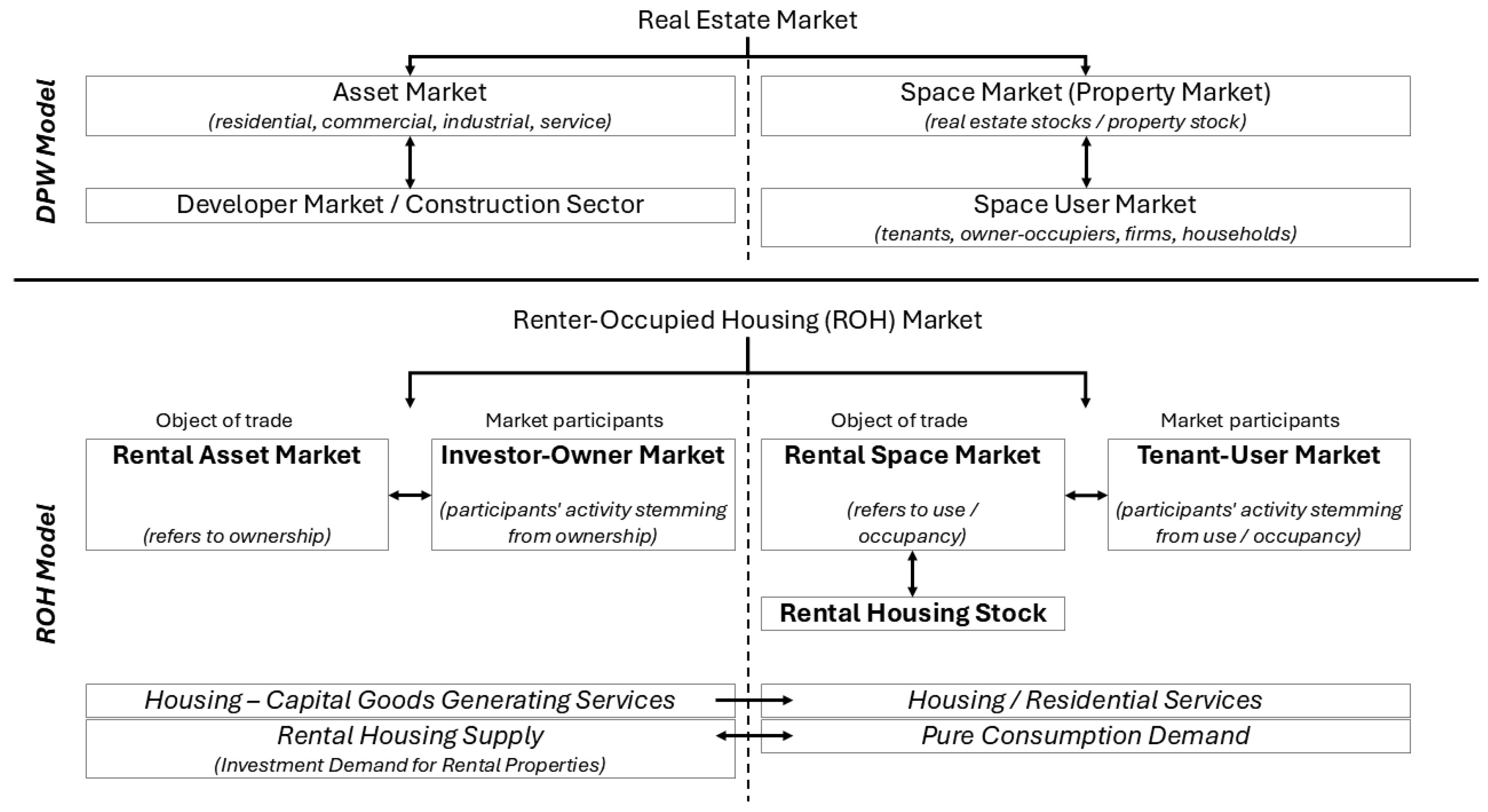
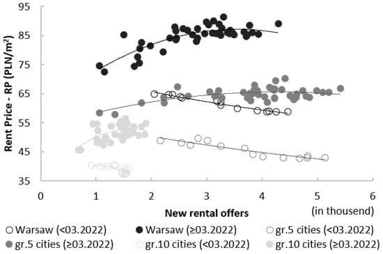
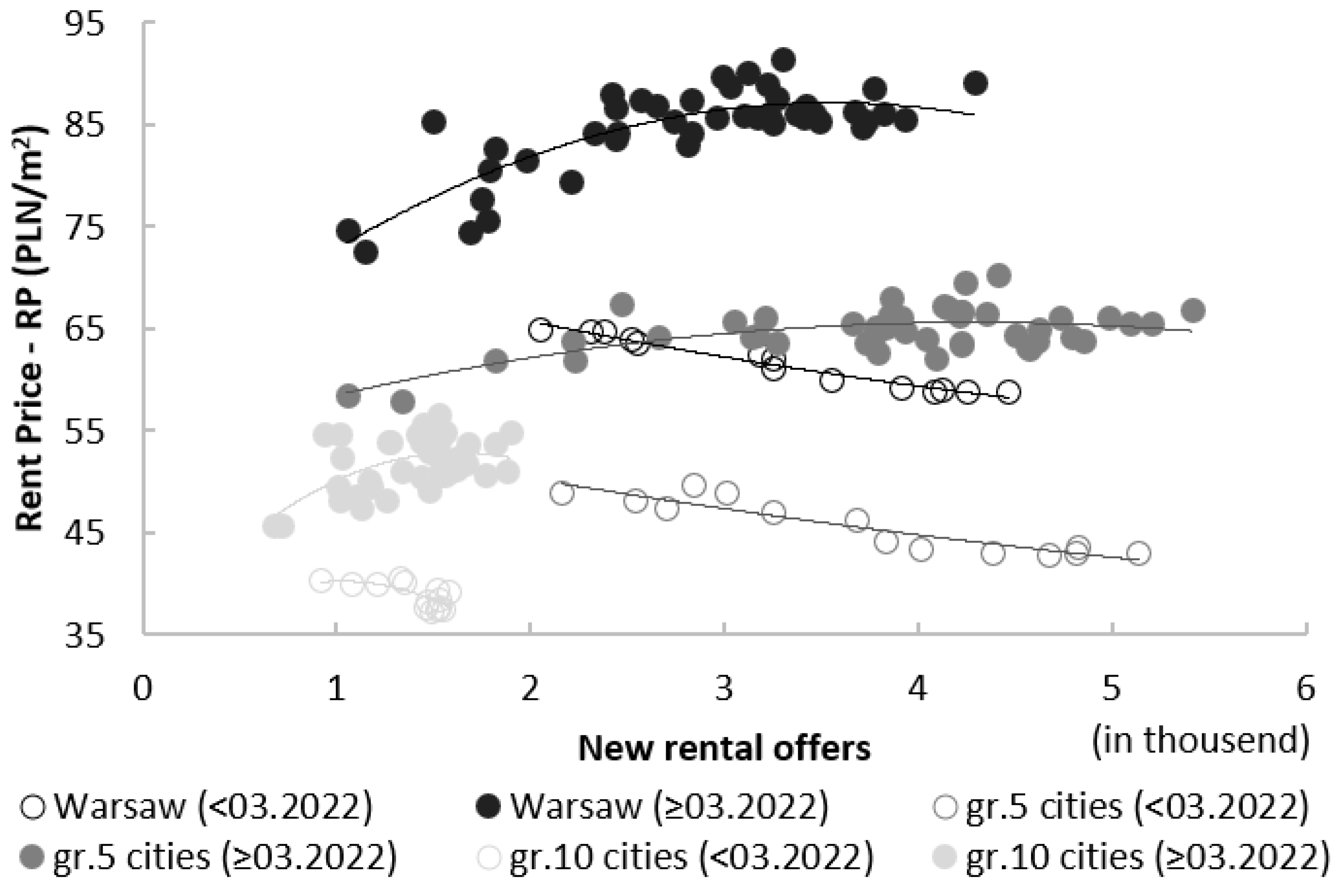
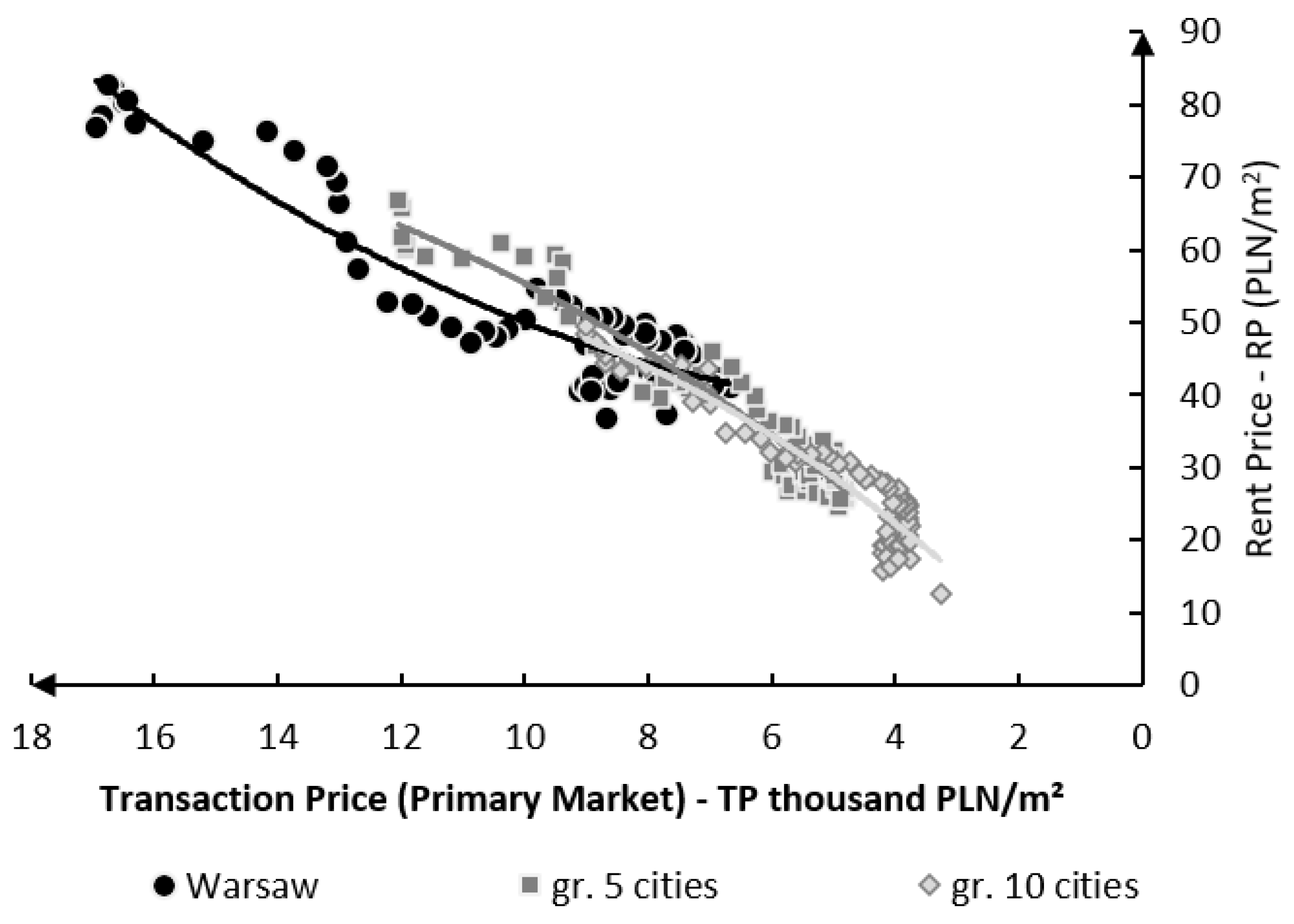
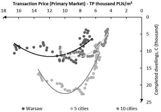
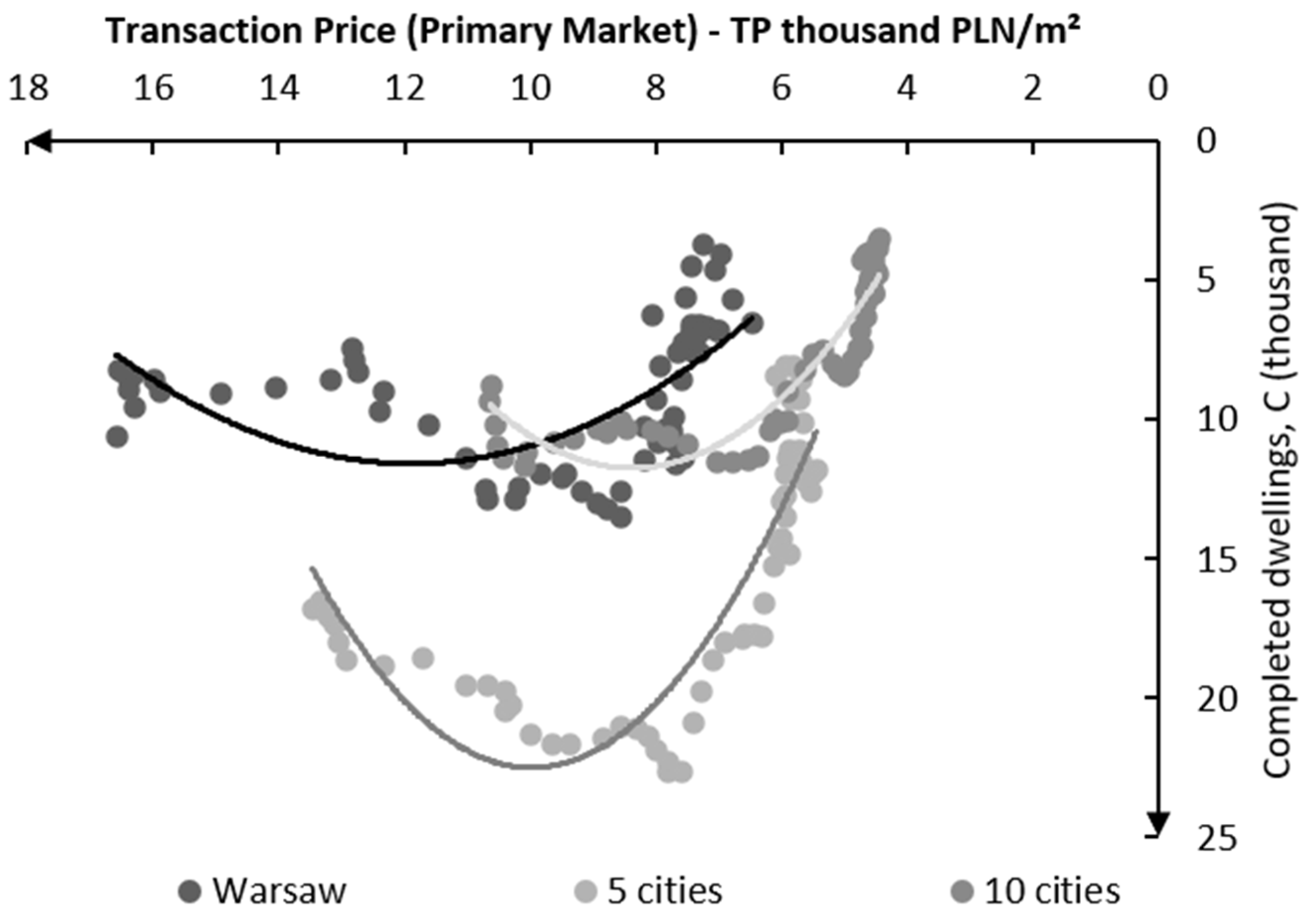
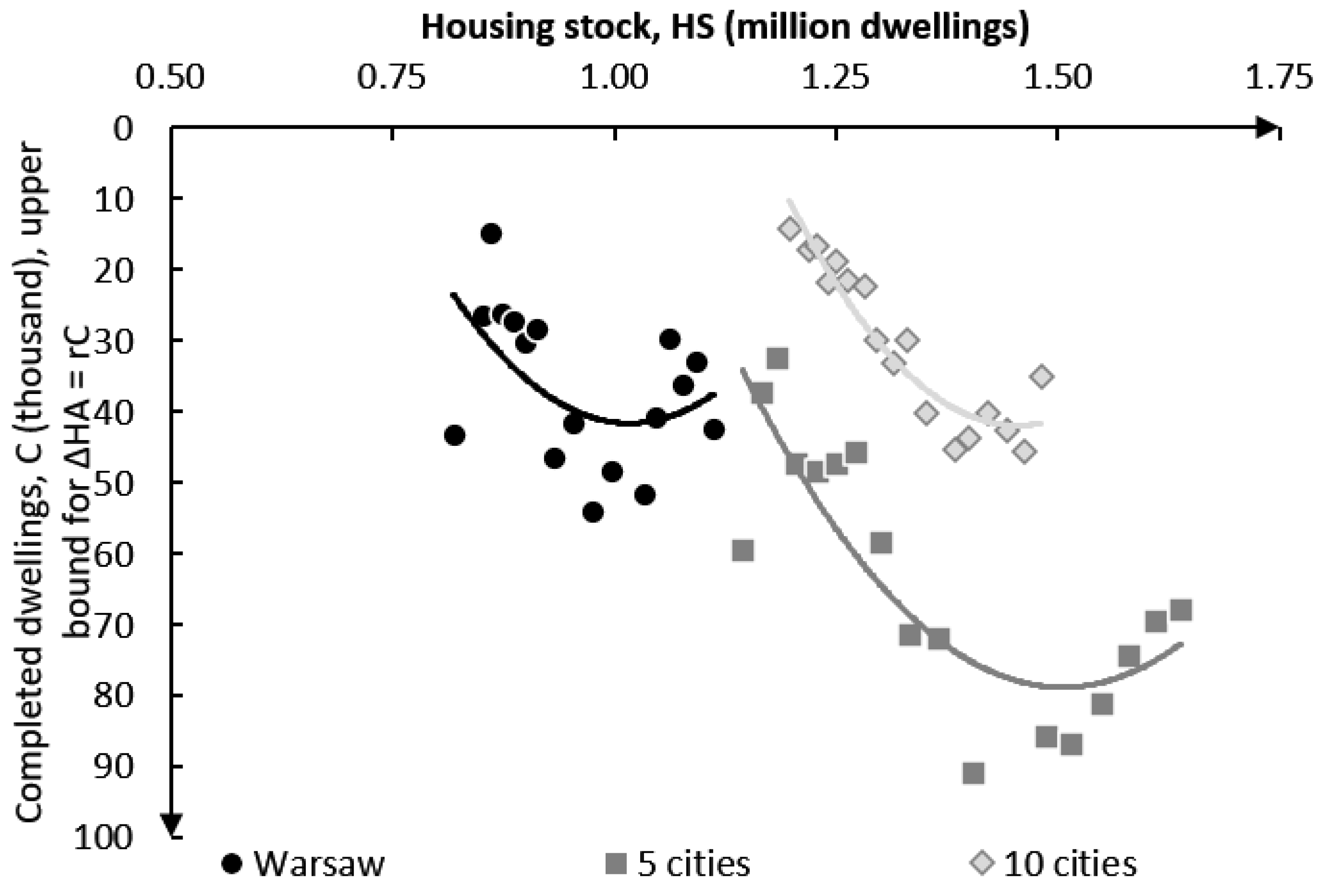

Disclaimer/Publisher’s Note: The statements, opinions and data contained in all publications are solely those of the individual author(s) and contributor(s) and not of MDPI and/or the editor(s). MDPI and/or the editor(s) disclaim responsibility for any injury to people or property resulting from any ideas, methods, instructions or products referred to in the content. |
© 2026 by the author. Licensee MDPI, Basel, Switzerland. This article is an open access article distributed under the terms and conditions of the Creative Commons Attribution (CC BY) license.