


Abstract
Time series analysis faces fundamental challenges when series contain trends, structural breaks, volatility, or anomalies that violate stationarity assumptions. Existing statistical tests produce inconsistent results on complex real-world patterns, while LLM and deep learning approaches lack comprehensive benchmarks for evaluating their understanding of diverse time series properties. We present BeTiSe, a large-scale synthetic benchmark that addresses these limitations through the controlled generation of series with well-documented characteristics. BeTiSe contains thousands of univariate time series across three length categories (short: 50–100, medium: 300–500, long: 1000–10,000 observations), generated to exhibit combinations of six fundamental properties: stationarity/non-stationarity, trends, seasonality, volatility dynamics, anomalies, and structural breaks. Each series is generated with explicit control over these characteristics and is accompanied by comprehensive metadata, including binary flags and detailed parameters for all applied transformations. We demonstrate BeTiSe’s utility through three applications: (1) neural network classifiers outperforming traditional tests (ADF, KPSS) in stationarity detection; (2) machine learning pipelines for the detection of trends, breaks, anomalies, and volatility; and (3) evaluation of the quality of the generated characteristics via visualization and statistical tests. BeTiSe is publicly available with complete documentation, generation code, and baseline results, supporting reproducible research across finance, economics, engineering, and the natural sciences.
1. Introduction
Time series data represents one of the most fundamental data types for capturing temporal changes in natural phenomena and economic, financial, or engineering processes. These data typically show some patterns of behavior, but in the presence of characteristics such as trends, seasonality, volatility, or structural breaks, the statistical properties can update over time. In such cases, even the most fundamental moments such as the mean and variance do not remain constant, making it hard to produce accurate forecasts with traditional means. Therefore, one of the most important steps in time series analysis is determining the properties of a series. Once they are clearly known, this information can be provided to forecasting models or Large Language Models (LLMs) to improve their performance. This study builds a generalized benchmark for time series datasets which consist of a large amount of resources covering a mixture of characteristics observed over time and synthetically produces short, medium, and long series to produce a common large-scale unified database for use under different controlled scenarios. With BeTiSe we offer a common framework that encapsulates the structural and statistical nature of each series through detailed metadata. This infrastructure is supposed to bridge the gap between traditional statistical foundations and the requirements of contemporary deep learning, also being a pivotal resource for training and verifying the development of new time-series-based foundation models (TSFMs).
Deciding to utilize synthetically generated data in BeTiSe comes from multiple methodological advantages that real-world datasets cannot provide. First, synthetic generation means an absolute ground truth for statistical properties that are usually impossible to track or ambiguous in empirical series. For instance, precisely knowing the exact point of a structural break or distinguishing between a collective and a contextual anomaly in real data is often subject to labeling bias. In addition, synthetic frameworks make isolation possible for different types of data, enabling researchers to better understand how individual characteristics, such as a cubic trend compared to a change in variance, affect model behavior in a controlled environment free from the noise of overlapping real-world phenomena. This degree of control is required for building a sound foundation for training and validating TSFMs. Moreover, this method effectively addresses the class imbalance challenges associated with practical anomaly detection by guaranteeing a balanced, broad, and diversified representation of all the scenarios found, thereby enabling more robust and generalizable temporal analysis.
In this work, we introduce BeTiSe, a large-scale, analytically grounded benchmark designed to enable rigorous evaluation of time-series structural and statistical properties that are fundamentally undetectable in real-world data. BeTiSe provides thousands of synthetically generated univariate time series with an explicit ground truth for stationarity, deterministic and stochastic trends, structural breaks, volatility dynamics, and diverse anomaly types, supported by a principled taxonomy and a controlled generation framework that allows systematic composition of complex temporal behaviors. Each series is accompanied by comprehensive metadata, including precise locations and parameters of anomalies and structural shifts, enabling fine-grained, property-aware evaluation across tasks such as stationarity testing, break localization, anomaly detection, and feature-based classification. Through extensive empirical studies, we demonstrate that BeTiSe exposes critical limitations of both classical statistical tests and modern learning-based models under non-stationary conditions, while also revealing substantial gaps in the temporal reasoning capabilities of contemporary LLMs in zero-shot settings. By providing a high-fidelity ground truth and a reusable evaluation infrastructure, BeTiSe establishes a foundation for the development, auditing, and benchmarking of next-generation time-series models beyond predictive accuracy alone.
2. Related Work
Benchmark datasets are crucial for identifying time series properties and evaluating forecasting models on real data. Many of the established databases combine real-world and synthetic data, enabling the training of contemporary time series foundation models.
2.1. Widely Used Benchmarks
Historically, the UCR and UEA Archives [1] provided the first standardized foundation for classification. For forecasting, the M-Competitions [2,3] and the Monash Repository [4] shifted the focus toward large-scale empirical data. More recently, initiatives such as the TS-Benchmark [5] have attempted to unify these tasks. However, these observational datasets often suffer from labeling ambiguity and a lack of precise control over underlying non-stationary shifts.
2.2. Statistical Foundations
Unit root tests such as Augmented Dickey–Fuller (ADF) [6], Phillips–Perron (PP) [7], and KPSS [8] are mainly used for classical stationarity analysis. Nevertheless, a large body of research indicates severe power and size issues with these tests. DeJong et al. [9] showed that the ADF and PP tests suffer from low power, where the null hypothesis of a unit root is often found when the series is stationary and highly autocorrelated but cannot be rejected. On the other hand, the KPSS test is prone to size distortion and often rejects stationarity in finite and high-frequency data. In addition, typical tests are often sensitive to structural breaks. Perron [10] demonstrated that stationary series with deterministic level shifts are often spuriously described as non-stationary using ADF-type tests. Although dedicated methods such as the Bai–Perron test [11] or Fourier-based unit root tests [12] attempt to deal with these shifts, they frequently require prior knowledge about break locations or involve high computational cost. BeTiSe fills these gaps with a mathematically oriented environment that contains the absolute ground truth for these characteristics. By providing time series with precisely controlled and fully documented statistical properties, BeTiSe enables researchers to rigorously evaluate and validate new detection, testing, and modeling methodologies against the known ground truth, something that is rarely achievable with real-world datasets where the true underlying structure remains unobservable.
2.3. Time Series Anomaly Detection (TSAD) Benchmarks
Many existing works aim to establish a unified, standardized, and scalable benchmarking environment for Time Series Anomaly Detection (TSAD) to address the “evaluation crisis” resulting from arbitrary metrics and inconsistent data. Schemes like TimeEval [13] and TSB-UAD [14] serve as automation pipelines for standardized testing, while Numenta Anomaly Benchmark (NAB) [15] and TSB-AD [16] present reliable scoring protocols. Reproducible learning is further promoted by integrated libraries such as Merlion [17] and specialized deep learning benchmarks such as TimeSeAD [18], Exathlon [19], and TSGBench [20]. To bridge the gap in evaluation consistency, Qiu et al. [21] recently introduced a unified framework. Within this ecosystem, deep generative and attention-based models have set new baselines, including stochastic recurrent networks such as OmniAnomaly [22], graph-based approaches such as Series2Graph [23], and the Anomaly Transformer [24]. Furthermore, unsupervised frameworks like DAGMM [25] have demonstrated the necessity of robust latent representations for identifying complex anomalies by jointly optimizing the parameters of the deep autoencoder and the mixture model.
2.4. Modern Time Series Architectures
In addition to recurrent and convolutional models like OmniAnomaly [22], which employs stochastic recurrent neural networks to model normal behavior and flag deviations in multivariate streams, and MSCRED [26], which builds multi-scale inter-sensor correlation matrices decoded via ConvLSTM to simultaneously detect and diagnose anomalies, recent architectures have set new performance standards by combining richer temporal representations with more principled uncertainty quantification. PatchTST [27] utilizes patching to capture local and global temporal contexts, while iTransformer [28] inverts the conventional Transformer architecture by applying self-attention across variates rather than time steps, enabling the model to capture multivariate correlations that are typically lost when attention is computed along the temporal dimension. TimesNet [29] addresses general time series analysis by reshaping 1D temporal sequences into 2D representations based on detected dominant periods, allowing 2D convolutional kernels to simultaneously capture both intraperiod (within-cycle) and interperiod (across-cycle) variations that a standard 1D treatment would conflate. More recently, diffusion-based models have emerged to tackle the unpredictability of non-stationary data, with NsDiff [30] providing a probabilistic approach to model distribution shifts over time. BeTiSe enables a rigorous evaluation of how these high-performance models recognize underlying statistical transitions beyond simple predictive accuracy.
2.5. Foundation Models and LLM-Based Time Series Analysis
Recent TSFMs such as Chronos [31], Moirai 2.0 [32], Sundial [33], TimesFM [34], and Lag-Llama [35] are trained on massive corpora that combine real-world data with synthetically generated series (e.g., via KernelSynth or TSMixup) to enhance generalization, underscoring the growing role of controlled synthetic data in model development. At the same time, recent empirical evaluations question their efficacy: single-layer linear models can surpass sophisticated Transformers in long-term forecasting [36], and TSFMs often fail to outperform traditional statistical methods or basic deep learning models in anomaly detection and zero-shot settings while incurring substantially higher computational costs [37,38]. Moreover, existing general-domain benchmarks are becoming saturated and fail to represent the diverse, labeled characteristics required to rigorously evaluate model robustness in real-world applications [37,39].
Closer to our focus, several recent works evaluate LLMs specifically on their ability to detect statistical characteristics of time series. Fons et al. [40] benchmark GPT-4 and related models on a taxonomy covering trends, structural breaks, volatility, and stationarity, finding that structural break and stationarity detection remain challenging across all models. Xie et al. [41] propose ChatTS, a multimodal LLM fine-tuned on synthetic time series with explicit attribute labels, demonstrating that targeted synthetic training substantially improves LLM understanding of such properties, while ReasonTSC [42] shows that LLMs can be steered to reason about fundamental time series characteristics to improve classification performance. However, these taxonomies remain descriptive and classification-oriented, and crucially provide no ground truth for the location or magnitude of the identified properties. Consistently, as shown in our zero-shot analysis of Qwen2.5, LLM-based models like Time-LLM [43] still struggle with core statistical constructs like structural breaks. BeTiSe directly addresses these gaps: it provides a precise, parameter-level ground truth for six statistically grounded properties, including GARCH-type volatility, mean/variance/trend shifts with exact change-point indices, and contextual anomalies, enabling evaluation at a level of rigor that descriptive taxonomies cannot support.
2.6. Taxonomy-Based Generation
Fons et al. [40] introduced a synthetic framework based on a taxonomy of features. However, there are remaining gaps in the literature. For instance, trends tend to be limited to standard up/down processes without regard for non-linear dynamics, and anomalies are often captured without the differentiation between contextual and collective types. Importantly, real-world data often contain overlapping characteristics, including non-linear trends, volatility, and point anomalies simultaneously, which are frequently absent in labeled datasets. BeTiSe bridges this crucial gap, providing a mathematically grounded environment in which these intricate behaviors are controlled precisely. Table 1 provides a feature-based comparison of BeTiSe with prominent time-series benchmarks.
Table 1.
Feature-based comparison of BeTiSe with prominent time-series benchmarks.
3. BeTiSe Framework
Our proposed framework generates synthetic univariate time series with various structural and statistical characteristics. The generator simulates behaviors by combining base processes, characteristics, and break types under controlled randomness. The taxonomy can be found in Table 2.
Table 2.
Taxonomy for the data generation plan.
3.1. Stationary Base Series
Stationary base series form the foundation upon which components are added. We utilize four types: White Noise (WN), Autoregressive (AR), Moving Average (MA), Autoregressive Moving Average (ARMA). The models used in time series generation can be observed in Table 3. The base series coefficients are sampled to ensure stationarity and invertibility; for example, AR coefficients are typically sampled from with the exclusion of the range to ensure statistically significant patterns.
Table 3.
Stationary series generation model.
3.2. Trend Components
To model long-term behavior, we implement several deterministic structures, each combined with random noise. Linear trends are generated with a randomly assigned direction and a slope adjusted to the series length, while quadratic trends exhibit parabolic growth controlled by curvature coefficients. Cubic trends produce S-shaped dynamics based on , and exponential trends capture growth or decline patterns shaped by vertical scale and rate parameters. Finally, damped trends represent directional patterns that gradually fade according to the formula given in Equation (1)
In addition to these deterministic forms, stochastic trends are created via the integration of stationary processes, using Random Walk (RW), RW with Drift, ARI, IMA, and ARIMA models. All trends are scaled relative to the series length L to maintain visual and statistical consistency across short (), medium (), and long () series.
3.3. Seasonality and Volatility
Seasonal behavior is generated via single-frequency sine waves, multi-frequency components, or seasonal models (SARIMA/SARMA). Volatility, in turn, is modeled using ARCH, GARCH, EGARCH, and APARCH frameworks to simulate time-varying variance clusters.
3.4. Anomalies and Structural Breaks
The framework distinguishes between transient anomalies and permanent behavioral changes (structural breaks). Anomalies include point anomalies (single or multiple isolated deviations), collective anomalies (consecutive deviations), and contextual anomalies (waveform inversions in seasonal patterns). Structural breaks, by contrast, comprise mean shifts (a permanent change in the average level), variance shifts (a change in the scale of fluctuations), and trend shifts (a sudden change in trajectory, magnitude, or both).
3.5. Experimental Setup
In the experiments, the samples are categorized by length: short (50–100), medium (300–500), and long (1000–10,000). Characteristics are generated in isolation or in complex n-tuple combinations. To ensure balance, stationary series are generated in equal proportion to non-stationary series, with each configuration resulting in 1000 samples.
4. Metadata and Data Management
The generated metadata captures the structural and statistical essence of each series to facilitate supervised learning. Specifically, the metadata include the following information:
- General Identifiers: Filename, series length, and global labels;
- Base Process Information: Underlying series type (e.g., AR, MA, White Noise), model order, and coefficient values;
- Deterministic Trends: Binary flags for linear (upward/downward), quadratic, cubic, exponential, and damped trends;
- Stochastic Trends: A single indicator for integrated processes;
- Seasonality: Indicators for presence, multiplicity, base model origin (e.g., SARMA/SAR-IMA), and frequency;
- Volatility: Flags for conditional heteroskedasticity processes such as ARCH or GARCH;
- Structural Breaks: Detailed fields for shifts in mean, variance, and trend, including the direction and support for multiple shift occurrences;
- Anomalies: Classification of point, collective, and contextual anomalies;
- Spatiotemporal Details: Storage of exact locations (indices) and magnitudes for every anomaly or structural break.
The full metadata column schema is documented in the project repository.
Beyond isolated properties, BeTiSe incorporates complex n-tuple combinations to reflect the multi-faceted nature of real-world observations. For instance, a single series may simultaneously exhibit a stochastic trend, structural breaks, and point anomalies, allowing models to learn and disentangle overlapping non-stationary characteristics effectively. The representative data generation templates for BeTiSe configuration, together with example figures of series generated with one and two characteristics, are provided in the project repository.
All numeric values are processed via a make_json_serializable utility to ensure compatibility. The generation framework is released as the open-source Python 3.11 package betise, available on PyPI (https://pypi.org/project/betise/ (accessed on 24 September 2026)), with the source code hosted on the project’s GitHub page (https://github.com/ismailguzel/betise (accessed on 24 September 2026)). The generation process produces data in Apache Parquet format, chosen for its efficiency and seamless mapping to CSV when required. The experiments detailed in the following sections were conducted using a collection generated by this script. To support research repeatability and provide a ready-to-use resource, the generated dataset is publicly available in CSV format via Zenodo (https://doi.org/10.5281/zenodo.18513505).
5. Quality Analysis of Generated Data
In order to validate the unique nature of the generated series, we conducted clustering and t-Distributed Stochastic Neighbor Embedding (t-SNE) analysis.
5.1. Clustering and Separability
We identified over 4200 short and 700 medium-length time series across 14 categories. All intervals were z-normalized prior to analysis. We used TimeSeriesKMeans created in the tslearn library and made use of Dynamic Time Warping (DTW) as the distance metric to consider temporal shifts. For the initial assessment, the number of clusters was set to k = 14. The clustering performance was assessed by three standard criteria metrics, yielding a Davies–Bouldin index of , a Calinski–Harabasz index of , and a silhouette score of on the constructed collection. This initial analysis suggests that while some meaningful groupings can be obtained, there are still significant overlaps, which hints at the difficulty of identifying such structures.
5.2. Visual Analysis via t-SNE
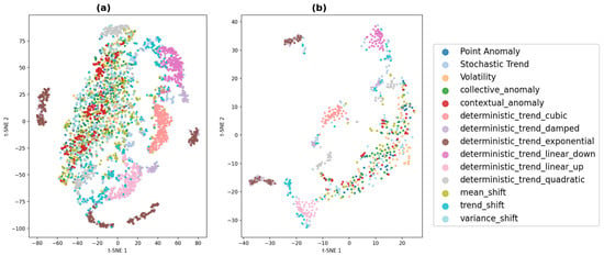
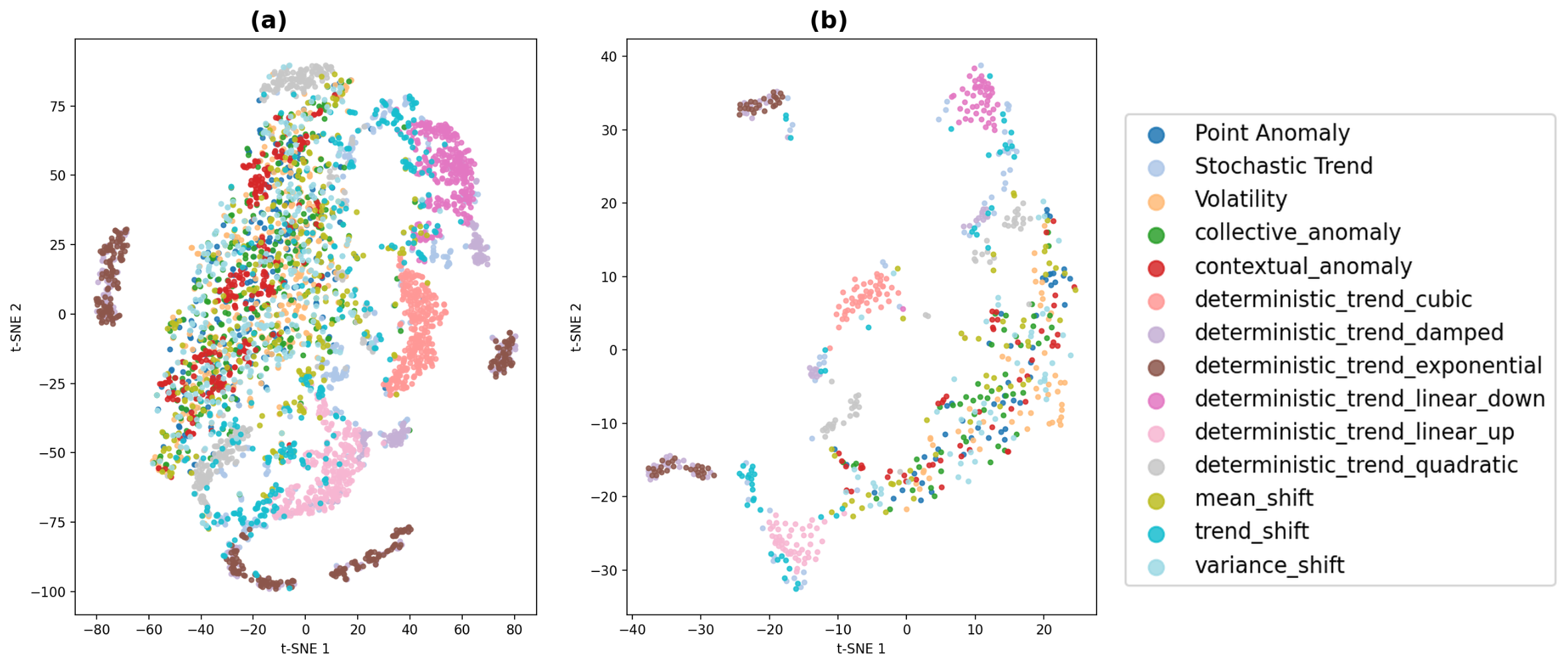
We used t-SNE to investigate the relationship in the DTW distance matrix. Anomaly types cluster in a two-dimensional space. Perplexity values around 10 and 20 produced the most interpretable results.
- Structural Shifts: Trend shift cases (represented in cyan) formed distinct clusters, providing evidence that the DTW metric effectively captures and distinguishes structural trajectory transitions.
- Deterministic Trends: While cubic trends (salmon pink) form well-defined clusters, damped and exponential patterns (gray and brown) cluster more closely due to similar global temporal behaviors. Despite these overlaps, deterministic trend categories remain largely distinguishable within the embedding space.
- Point Anomalies: These instances (blue) appeared scattered throughout the space rather than forming a single cluster. This indicates that localized anomalies do not form cohesive groups when evaluated using global distance metrics like DTW, highlighting a significant detection challenge for traditional proximity-based methods.
For medium-length series, the separation became more pronounced, achieving a silhouette score of 0.262 and a Calinski–Harabasz index of 251,096.0. This indicates that longer temporal contexts allow for better differentiation between statistical shifts (e.g., mean and variance) and deterministic trends. The results for short and medium series are illustrated in Figure 1a, b, respectively.
Figure 1.
t-SNE embeddings computed using DTW distances, colored by true label: (a) short series (perplexity = 10); (b) medium series (perplexity = 20).
6. Distributional Similarity Analysis
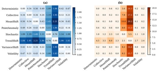
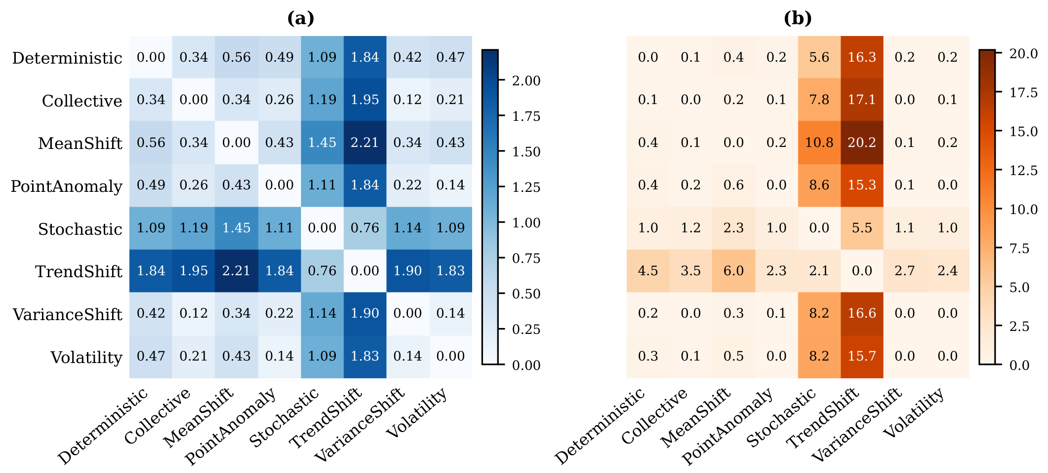
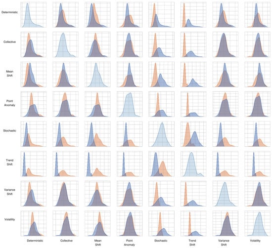
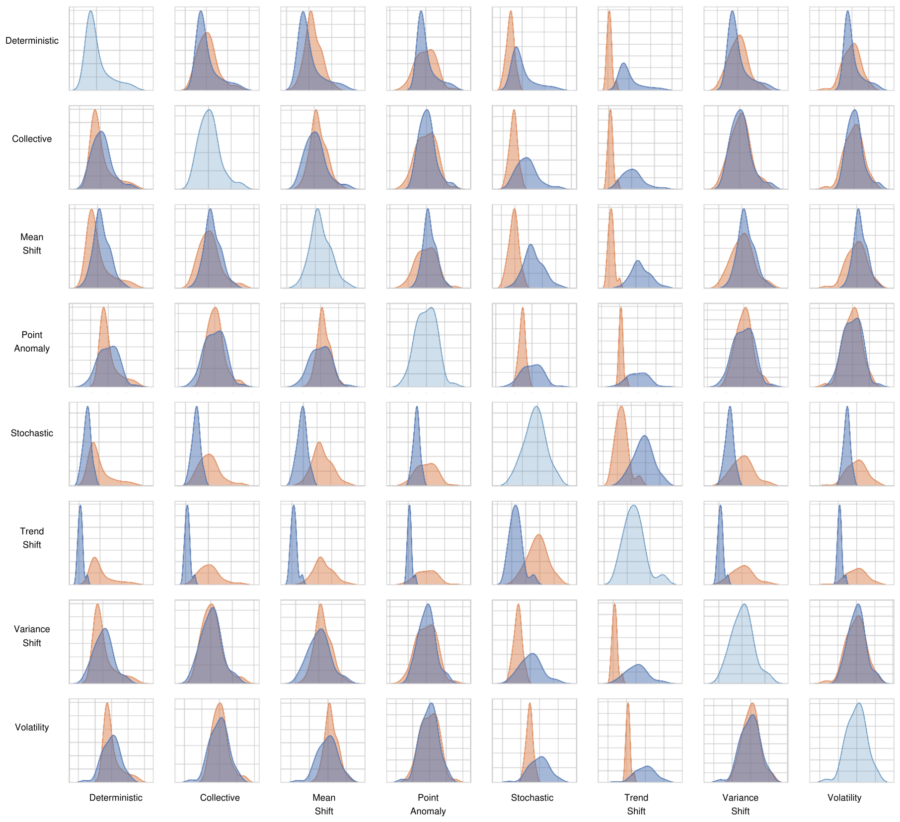
We further quantified these differences using the Wasserstein distance and the Kullback–Leibler (KL) divergence. According to pairwise Wasserstein distances, trend-based shifts are outliers to other classes, whereas variance and volatility distances are quite small (see Figure 2a). The KL divergence was used as an asymmetric measure to determine how well one class distribution represents another; small epsilon values were added to prevent calculation errors in regions with zero probability. The pairwise KL divergence heatmap for the representative eight classes is shown in Figure 2b. Finally, an kernel density estimation (KDE) matrix, as shown in Figure 3, was constructed to compare class distributions. The analysis revealed that while “trend shift” is easily distinguishable, classes like “variance shift”, “volatility”, and “collective anomaly” exhibit significant overlap. This difficulty in separation is consistent with the theoretical definitions of these processes.
Figure 2.
Distributional similarity analysis for the selected eight classes: (a) pairwise Wasserstein distance heatmap; (b) pairwise KL divergence heatmap.
Figure 3.
Pairwise KDE comparisons. Blue and orange curves represent the KDEs of the row and column classes, respectively.
The structural integrity and reliability of the generated series are validated through a robust, multi-faceted quality assessment. Clustering analysis using DTW and t-SNE visualizations shows clear separability for structural shifts and deterministic trends, while overlaps among closely related classes remain, consistent with the moderate clustering scores reported above. Furthermore, distributional similarity checks using Wasserstein distance and KL divergence confirm the distinctiveness of the generated classes, verifying that the series are both mathematically sound and theoretically consistent. Finally, the exceptional performance of baseline machine learning models, achieving F1-scores of up to 0.9410 for stationarity detection (see Section 7), provides conclusive evidence of the dataset’s superior labeling quality and its capacity to serve as a high-fidelity benchmark for complex temporal analysis.
7. Baseline Classification Performance
To evaluate the discriminatory power and label quality of the BeTiSe dataset, we conducted a rigorous baseline analysis using nine distinct machine learning algorithms. These models, ranging from traditional ensemble methods including Random Forest, XGBoost, and Extra Trees to neural network architectures such as the Multi-Layer Perceptron (MLP), were evaluated on a comprehensive test set of 119,123 samples. The primary objective of this investigation is to establish a performance benchmark for identifying stationarity and local structural breaks within complex temporal sequences.
7.1. Feature Engineering
The features were extracted using a sliding window approach with three scales: , , and (where L is the series length). The extracted features comprise statistical descriptors (mean, standard deviation, and quantiles), temporal characteristics (autocorrelation and seasonality components), and frequency-domain information (Fast Fourier Transform (FFT) coefficients).
7.2. Results
For stationarity detection, the MLP model achieved the highest -score of using the window size, as seen in Table 4. For mean shift detection, LightGBM outperformed the other models with an -score of on a balanced dataset of 96,000 samples; the results can be seen in Table 5.
Table 4.
Model performances for stationarity detection with window size and hyperparameter optimization (: Cohen’s kappa; MCC: Matthews correlation coefficient).
Table 5.
Model performances of mean shift detection with window size. Computation times were measured on a 2022 Apple MacBook Pro (Apple Inc., Cupertino, CA, USA).
7.3. Comparison with Classical Stationarity Tests
To contextualize the learning-based results, we also applied the ADF and KPSS tests to balanced sets of stationary and non-stationary BeTiSe series. The ADF test attains an overall accuracy of (): while it correctly flags of the non-stationary series, it misclassifies of the truly stationary series as non-stationary. The KPSS test performs slightly better, with an accuracy of (), yet it still mislabels more than half of the stationary series ( specificity). These results empirically confirm the power and size issues of classical tests discussed in Section 2.2, and contrast sharply with the learning-based classifiers in Table 4, demonstrating the value of BeTiSe’s exact ground truth for quantifying such failure modes.
7.4. Assessment of Label Discriminatory Power via High-Dimensional Feature Extraction
To thoroughly validate the quality of the BeTiSe dataset, we developed a specialized machine learning pipeline to detect eight distinct characteristic categories under non-stationary conditions—namely, trend: (1) deterministic and (2) stochastic; structural break: (3) mean shift, (4) variance shift, and (5) trend shift; (6) volatility; anomalies: (7) point anomaly and (8) collective anomaly. Due to the distinct nature of seasonality and the inclusion of contextual anomalies within its structure, these cases were omitted from the current analysis. We generated 10 sub-datasets by repeatedly sampling from our main data. Each set was tested for stationarity using ADF and KPSS tests. If a set was non-stationary, we applied the same tests to identify whether its trend was deterministic or stochastic. Unlike traditional sliding-window algorithms, this framework treats each time series as an entire sequence, extracting 777 statistical, spectral, and temporal features using the tsfresh “Efficient” parameter set.
This high-dimensional feature space enables models to capture the distinct underlying characteristics of each class. We employed an Ensemble One-vs-Rest (OvR) strategy, training eight binary classifiers. For each category, the optimal model was dynamically selected from a pool of LightGBM, XGBoost, and MLP architectures based on F1-score performance. Including all eight categories degraded the model’s performance; consequently, some sub-categories were consolidated into a single main category. The resulting LightGBM model (configured with n_estimators = 300 and class_weight = ’balanced’) consistently outperformed other architectures.
As shown in Table 6, the results demonstrate near-perfect separability for classes such as deterministic trend, while providing a challenging but robust benchmark for more complex structures, such as point and collective anomalies. These findings confirm that the synthetic generation process exhibits high inter-class variance and strong internal consistency.
Table 6.
Class-wise performance metrics for characteristic detection (LightGBM OvR pipeline), sorted by -score within each category.
7.5. Zero-Shot Evaluation of Large Language Models (LLMs)
To evaluate contemporary foundation models for performance when it comes to temporal dynamics, we evaluated the open-weight Qwen2.5 model (7B parameters, executed locally via Ollama) on two zero-shot classification problems based on BeTiSe samples. This model was deliberately chosen as a small, widely accessible baseline so that the evaluation can be reproduced on commodity hardware without relying on proprietary APIs. The full prompt templates used in this analysis are available in the project repository.
7.5.1. Binary Stationarity Detection
Using a balanced test set of 3000 series, the LLM achieved an overall accuracy of 52.53%. The model demonstrated high sensitivity to non-stationary patterns (0.78 recall); however, it exhibited a strong bias, with stationary series frequently classified as non-stationary (0.27 recall).
7.5.2. Multi-Class Feature Identification
We set a more advanced problem that enabled the model to recognize the most salient characteristic of the five classes, such as deterministic trend, stochastic trend, structural break, volatility, and anomaly. The proposed model attained an accuracy of only 31.36% from 7500 series. The findings illustrate a fundamental shortcoming: although LLMs achieve some degree of success with semantically based temporal terms such as anomalies (0.88 recall), they fail to identify statistical expressions like structural breaks (0% recall) and show poor ability to detect volatility. The findings indicate that existing TSFMs need the high fidelity of ground truth of BeTiSe to tailor for the relevant fine-tuning.
8. Limitations
BeTiSe does present a stable and controlled environment for evaluating time series characteristics, but a few shortcomings persist that present avenues for future inquiry.
8.1. The Synthetic-to-Real Domain Gap
The primary methodological limitation of BeTiSe is the inherent nature of its analytically generated datasets. Synthetic generation guarantees ground truth for typically undetectable properties such as structural breaks and precise anomaly locations and may not capture the latent complexities, noise-to-signal ratios, or irregular sampling intervals common in naturalistic settings. Models that achieve high performance on BeTiSe will need more domain adaptation to remain efficient on noisy and empirical data when valid underlying properties frequently overlap and become less distinct.
8.2. Univariate Scope
BeTiSe is limited to univariate time series at present. While this enables the isolation and precise study of fundamental properties such as stationarity and specific trend types, it does not address the cross-correlations and inter-variable dependencies that are inherent to multivariate systems. Therefore, the benchmark cannot at present assess models tailored for high-dimensional sensor networks or multi-agent systems where anomalies can only present themselves through inter-channel relationships.
9. Conclusions and Future Work
In this work, we introduced BeTiSe, a novel, large-scale synthetic benchmarking framework designed to establish a new gold standard of methodological robustness, rigor, and transparency in time-series research. Providing an analytically deep, detailed taxonomy of several basic properties (including non-stationarity, complex volatility clusters, and contextual anomalies), BeTiSe fills the gap between classical statistical rigor and the demands of contemporary deep learning. Rather than relying on task-specific datasets, our benchmark offers a high-fidelity ground truth over undetectable characteristics, and therefore, a standard which allows for a more accurate evaluation of models for detecting temporal dynamics based not just on their prediction accuracy, but also on their basic knowledge of the temporal dynamics of the system.
The usefulness of BeTiSe is not limited to traditional machine learning; our zero-shot analyses in LLMs clearly expose a key capability gap in temporal reasoning. While models like Qwen2.5 exhibit moderate sensitivity to semantic ideas like anomalies, they inherently have difficulties with significant statistical constructs, such as the fact that they fail to recall structural breaks (0.00 recall) and show poor ability to detect volatility, versus the exceptional performance of dedicated neural classification methods. This validates that BeTiSe provides the necessary infrastructure to audit and calibrate subsequent TSFMs.
Future research will expand this framework to multivariate systems, focusing on deep learning solutions for disentangling overlapping anomalies, such as concurrent point and collective shifts. BeTiSe establishes the transparency and reproducibility required to advance the state-of-the-art in robust and generalizable temporal AI.
Author Contributions
Conceptualization, C.Y., İ.G. and P.K.; methodology, İ.G., P.K. and C.Y.; software, K.G., P.Y., P.E., Y.T. and B.B.; validation, İ.G. and P.K.; formal analysis, K.G., P.Y., P.E., Y.T. and B.B.; investigation, K.G., P.Y., P.E., Y.T. and B.B.; data curation, K.G., P.Y., P.E., Y.T. and B.B.; writing—original draft preparation, K.G., P.Y., P.E., Y.T. and B.B.; writing—review and editing, İ.G., P.K. and C.Y.; visualization, K.G., P.Y., P.E., Y.T. and B.B.; supervision, C.Y., İ.G. and P.K.; project administration, C.Y.; funding acquisition, C.Y. All authors have read and agreed to the published version of the manuscript.
Funding
This research was funded by the Scientific and Technological Research Council of Türkiye (TÜBİTAK) grant number 124F095 and the Middle East Technical University (METU) Scientific Research Projects Coordination Unit grant number GAP-109-2023-11361.
Institutional Review Board Statement
Not applicable.
Informed Consent Statement
Not applicable.
Data Availability Statement
The dataset generated in this study is publicly available in CSV format via Zenodo at https://doi.org/10.5281/zenodo.18513505. The generation code is available as the betise Python package on PyPI (https://pypi.org/project/betise/ (accessed on 24 September 2026)) and on GitHub (https://github.com/ismailguzel/betise (accessed on 24 September 2026)).
Acknowledgments
During the preparation of this manuscript, the authors used Claude 3.7 Sonnet (Anthropic) for the purposes of English language and grammar editing. The authors have reviewed and edited the output and take full responsibility for the content of this publication.
Conflicts of Interest
The authors declare no conflicts of interest.
Abbreviations
The following abbreviations are used in this manuscript:
| ADF | Augmented Dickey–Fuller |
| AR | Autoregressive |
| ARCH | Autoregressive Conditional Heteroskedasticity |
| ARIMA | Autoregressive Integrated Moving Average |
| ARMA | Autoregressive Moving Average |
| DTW | Dynamic Time Warping |
| FFT | Fast Fourier Transform |
| GARCH | Generalized Autoregressive Conditional Heteroskedasticity |
| KDE | Kernel Density Estimation |
| KL | Kullback–Leibler |
| KPSS | Kwiatkowski–Phillips–Schmidt–Shin |
| LLM | Large Language Model |
| MA | Moving Average |
| MCC | Matthews Correlation Coefficient |
| MLP | Multi-Layer Perceptron |
| OvR | One-vs-Rest |
| PP | Phillips–Perron |
| RW | Random Walk |
| SARIMA | Seasonal ARIMA |
| TSAD | Time Series Anomaly Detection |
| TSFM | Time Series Foundation Model |
| t-SNE | t-Distributed Stochastic Neighbor Embedding |
| WN | White Noise |
References
- Dau, H.A.; Bagnall, A.; Kamgar, K.; Yeh, C.C.M.; Zhu, Y.; Gharghabi, S.; Ratanamahatana, C.A.; Keogh, E. The UCR Time Series Archive. IEEE/CAA J. Autom. Sin. 2019, 6, 1293–1305. [Google Scholar] [CrossRef] [Scilit]
- Makridakis, S.; Spiliotis, E.; Assimakopoulos, V. The M4 Competition: Results, findings, conclusion and way forward. Int. J. Forecast. 2018, 34, 802–808, Erratum in Int. J. Forecast. 2021, 37, 1308–1309. [Google Scholar] [CrossRef] [Scilit]
- Makridakis, S.; Spiliotis, E.; Assimakopoulos, V. The M5 accuracy competition: Results, findings, and conclusions. Int. J. Forecast. 2022, 38, 1346–1364. [Google Scholar] [CrossRef] [Scilit]
- Godahewa, R.; Bergmeir, C.; Webb, G.I.; Hyndman, R.J.; Montero-Manso, P. Monash Time Series Forecasting Archive. In Proceedings of the 35th Conference on Neural Information Processing Systems (NeurIPS 2021), Datasets and Benchmarks Track, Virtual, 6–14 December 2021. [Google Scholar]
- Hao, Y.; Qin, X.; Chen, Y.; Li, Y.; Sun, X.; Tao, Y.; Zhang, X.; Du, X. TS-Benchmark: A Benchmark for Time Series Databases. In Proceedings of the 2021 IEEE 37th International Conference on Data Engineering (ICDE), Chania, Greece, 19–22 April 2021; pp. 588–599. [Google Scholar] [CrossRef] [Scilit]
- Dickey, D.A.; Fuller, W.A. Likelihood Ratio Statistics for Autoregressive Time Series with a Unit Root. Econometrica 1981, 49, 1057–1072. [Google Scholar] [CrossRef] [Scilit]
- Phillips, P.C.B.; Perron, P. Testing for a unit root in time series regression. Biometrika 1988, 75, 335–346. [Google Scholar] [CrossRef]
- Kwiatkowski, D.; Phillips, P.C.B.; Schmidt, P.; Shin, Y. Testing the null hypothesis of stationarity against the alternative of a unit root. J. Econom. 1992, 54, 159–178. [Google Scholar] [CrossRef] [Scilit]
- DeJong, D.N.; Nankervis, J.C.; Savin, N.E.; Whiteman, C.H. The power problems of unit root test in time series with autoregressive errors. J. Econom. 1992, 53, 323–343. [Google Scholar] [CrossRef] [Scilit]
- Perron, P. The Great Crash, the Oil Price Shock, and the Unit Root Hypothesis. Econometrica 1989, 57, 1361–1401. [Google Scholar] [CrossRef] [Scilit]
- Bai, J.; Perron, P. Estimating and Testing Linear Models with Multiple Structural Changes. Econometrica 1998, 66, 47–78. [Google Scholar] [CrossRef] [Scilit]
- Becker, R.; Enders, W.; Lee, J. A stationarity test in the presence of an unknown number of smooth breaks. J. Time Ser. Anal. 2006, 27, 381–409. [Google Scholar] [CrossRef] [Scilit]
- Wenig, P.; Schmidl, S.; Papenbrock, T. TimeEval: A Benchmarking Toolkit for Time Series Anomaly Detection Algorithms. Proc. VLDB Endow. 2022, 15, 3678–3681. [Google Scholar] [CrossRef] [Scilit]
- Paparrizos, J.; Kang, Y.; Boniol, P.; Tsay, R.S.; Palpanas, T.; Franklin, M.J. TSB-UAD: An end-to-end benchmark suite for univariate time-series anomaly detection. Proc. VLDB Endow. 2022, 15, 1697–1711. [Google Scholar]
- Ahmad, S.; Lavin, A.; Purdy, S.; Agha, Z. Unsupervised real-time anomaly detection for streaming data. Neurocomputing 2017, 262, 134–147. [Google Scholar] [CrossRef] [Scilit]
- Liu, Q.; Paparrizos, J. The Elephant in the Room: Towards A Reliable Time-Series Anomaly Detection Benchmark. In Proceedings of the Advances in Neural Information Processing Systems (NeurIPS), Vancouver, BC, Canada, 10–15 December 2024; Volume 37, pp. 108231–108261. [Google Scholar]
- Bhatnagar, A.; Kassianik, P.; Liu, C.; Lan, T.; Yang, W.; Cassius, R.; Sahoo, D.; Arpit, D.; Subramanian, S.; Woo, G.; et al. Merlion: A Machine Learning Library for Time Series. arXiv 2021, arXiv:2109.09265. [Google Scholar]
- Wagner, D.; Michels, T.; Schulz, F.C.F.; Nair, A.; Rudolph, M.; Kloft, M. TimeSeAD: Benchmarking Deep Multivariate Time-Series Anomaly Detection. Trans. Mach. Learn. Res. 2023. Available online: https://openreview.net/forum?id=iMmsCI0JsS (accessed on 6 September 2026).
- Jacob, V.; Song, F.; Stiegler, A.; Rad, B.; Diao, Y.; Tatbul, N. Exathlon: A Benchmark for Explainable Anomaly Detection over Time Series. Proc. VLDB Endow. 2021, 14, 2613–2626. [Google Scholar] [CrossRef] [Scilit]
- Ang, Y.; Huang, Q.; Bao, Y.; Tung, A.K.H.; Huang, Z. TSGBench: Time Series Generation Benchmark. Proc. VLDB Endow. 2023, 17, 305–318. [Google Scholar] [CrossRef] [Scilit]
- Qiu, X.; Li, Z.; Qiu, W.; Hu, S.; Zhou, L.; Wu, X.; Li, Z.; Guo, C.; Zhou, A.; Sheng, Z.; et al. TAB: Unified Benchmarking of Time Series Anomaly Detection Methods. Proc. VLDB Endow. 2025, 18, 1–14. [Google Scholar] [CrossRef] [Scilit]
- Su, Y.; Zhao, Y.; Niu, C.; Liu, R.; Sun, W.; Pei, D. Robust Anomaly Detection for Multivariate Time Series through Stochastic Recurrent Neural Network. In Proceedings of the 25th ACM SIGKDD International Conference on Knowledge Discovery & Data Mining, Anchorage, AK, USA, 4–8 August 2019; pp. 2828–2837. [Google Scholar]
- Boniol, P.; Palpanas, T. Series2Graph: Graph-based Subsequence Anomaly Detection for Time Series. Proc. VLDB Endow. 2020, 13, 1821–1834. [Google Scholar]
- Xu, J.; Wu, H.; Wang, J.; Long, M. Anomaly Transformer: Time Series Anomaly Detection with Association Discrepancy. In Proceedings of the International Conference on Learning Representations (ICLR), Virtual, 25–29 April 2022. [Google Scholar]
- Zong, B.; Song, Q.; Min, M.R.; Cheng, W.; Lumezanu, C.; Cho, D.k.; Chen, H. Deep Autoencoding Gaussian Mixture Model for Unsupervised Anomaly Detection. In Proceedings of the International Conference on Learning Representations, Vancouver, BC, Canada, 30 April–3 May 2018. [Google Scholar]
- Zhang, C.; Song, D.; Chen, Y.; Feng, X.; Lumezanu, C.; Cheng, W.; Ni, J.; Zong, B.; Chen, H.; Chawla, N.V. A Deep Neural Network for Unsupervised Anomaly Detection and Diagnosis in Multivariate Time Series Data. In Proceedings of the AAAI Conference on Artificial Intelligence, Honolulu, HI, USA, 27 January–1 February 2019; Volume 33, pp. 1409–1416. [Google Scholar]
- Nie, Y.; Nguyen, N.H.; Sinthong, P.; Kalagnanam, J. A Time Series is Worth 64 Words: Long-term Forecasting with Transformers. In Proceedings of the International Conference on Learning Representations (ICLR), Kigali, Rwanda, 1–5 May 2023. [Google Scholar]
- Liu, Y.; Hu, T.; Zhang, H.; Wu, H.; Wang, S.; Ma, L.; Long, M. iTransformer: Inverted Transformers are Effective for Time Series Forecasting. In Proceedings of the International Conference on Learning Representations (ICLR), Vienna, Austria, 7–11 May 2024. [Google Scholar]
- Wu, H.; Hu, T.; Liu, Y.; Zhou, H.; Wang, J.; Long, M. TimesNet: Temporal 2D-Variation Modeling for General Time Series Analysis. In Proceedings of the International Conference on Learning Representations (ICLR), Kigali, Rwanda, 1–5 May 2023. [Google Scholar]
- Ye, W.; Xu, Z.; Gui, N. Non-stationary Diffusion for Probabilistic Time Series Forecasting. In Proceedings of the 42nd International Conference on Machine Learning (ICML), Vancouver, BC, Canada, 13–19 July 2025. [Google Scholar]
- Ansari, A.F.; Stella, L.; Turkmen, C.; Zhang, X.; Mercado, P.; Shen, H.; Shchur, O.; Rangapuram, S.S.; Arango, S.P.; Kapoor, S.; et al. Chronos: Learning the Language of Time Series. arXiv 2024, arXiv:2403.07815. [Google Scholar]
- Liu, C.; Aksu, T.; Liu, J.; Liu, X.; Yan, H.; Pham, Q.; Savarese, S.; Sahoo, D.; Xiong, C.; Li, J. Moirai 2.0: When Less Is More for Time Series Forecasting. arXiv 2026, arXiv:2511.11698. [Google Scholar]
- Liu, Y.; Qin, G.; Shi, Z.; Chen, Z.; Yang, C.; Huang, X.; Wang, J.; Long, M. Sundial: A Family of Highly Capable Time Series Foundation Models. arXiv 2025, arXiv:2502.00816. [Google Scholar] [CrossRef] [Scilit]
- Das, A.; Kong, W.; Sen, R.; Zhou, Y. A decoder-only foundation model for time-series forecasting. arXiv 2024, arXiv:2310.10688. [Google Scholar] [CrossRef] [Scilit]
- Rasul, K.; Ashok, A.; Williams, A.R.; Ghonia, H.; Bhagwatkar, R.; Khorasani, A.; Darvishi Bayazi, M.J.; Adamopoulos, G.; Riachi, R.; Hassen, N.; et al. Lag-Llama: Towards Foundation Models for Probabilistic Time Series Forecasting. arXiv 2024, arXiv:2310.08278. [Google Scholar]
- Zeng, A.; Chen, M.; Zhang, L.; Xu, Q. Are Transformers Effective for Time Series Forecasting? arXiv 2022, arXiv:2205.13504. [Google Scholar]
- Shyalika, C.; Bagga, H.K.; Bhatt, A.; Prasad, R.; Al Ghazo, A.; Sheth, A. Time Series Foundational Models: Their Role in Anomaly Detection and Prediction. arXiv 2024, arXiv:2412.19286. [Google Scholar]
- Toner, W.; Lee, T.L.; Joosen, A.; Singh, R.; Asenov, M. Performance of Zero-Shot Time Series Foundation Models on Cloud Data. arXiv 2025, arXiv:2502.12944. [Google Scholar]
- Ma, Q.; Shi, J.; Qiu, J.; Yang, Z. Position: The Inevitable End of One-Architecture-Fits-All-Domains in Time Series Forecasting. arXiv 2026, arXiv:2602.01736. [Google Scholar]
- Fons, E.; Kaur, R.; Palande, S.; Zeng, Z.; Balch, T.; Veloso, M.; Vyetrenko, S. Evaluating Large Language Models on Time Series Feature Understanding: A Comprehensive Taxonomy and Benchmark. In Proceedings of the 2024 Conference on Empirical Methods in Natural Language Processing, Miami, FL, USA, 12–16 November 2024; pp. 21598–21634. [Google Scholar]
- Xie, Z.; Li, Z.; He, X.; Xu, L.; Wen, X.; Zhang, T.; Chen, J.; Pei, D. ChatTS: Aligning Time Series with LLMs via Synthetic Data for Enhanced Understanding and Reasoning. Proc. VLDB Endow. 2025, 18, 2385–2398. [Google Scholar] [CrossRef] [Scilit]
- Zhou, J.; Li, D.; Li, L.; Chen, Z.; Wu, S.; Ye, H.; Lou, J.; Spanos, C.J. Enhancing LLM Reasoning for Time Series Classification by Tailored Thinking and Fused Decision. arXiv 2025, arXiv:2506.00807. [Google Scholar]
- Jin, M.; Wang, S.; Ma, L.; Chu, Z.; Zhang, J.Y.; Shi, X.; Chen, P.Y.; Liang, Y.; Li, Y.F.; Pan, S.; et al. Time-LLM: Time Series Forecasting by Reprogramming Large Language Models. In Proceedings of the International Conference on Learning Representations (ICLR), Vienna, Austria, 7–11 May 2024. [Google Scholar]

Disclaimer/Publisher’s Note: The statements, opinions and data contained in all publications are solely those of the individual author(s) and contributor(s) and not of MDPI and/or the editor(s). MDPI and/or the editor(s) disclaim responsibility for any injury to people or property resulting from any ideas, methods, instructions or products referred to in the content. |
© 2026 by the authors. Licensee MDPI, Basel, Switzerland. This article is an open access article distributed under the terms and conditions of the Creative Commons Attribution (CC BY) license.