Optimization Sensitivity in ARFIMA and FIGARCH Models for Precious Metals ^†

Abstract

This study evaluates parameter estimation sensitivity in long-memory time series models, focusing on the Autoregressive Fractionally Integrated Moving Average (ARFIMA) and the Fractionally Integrated Generalized Autoregressive Conditional Heteroskedasticity (FIGARCH) models. The optimization techniques applied in the models utilized the daily logarithmic returns of four precious metals traded on the Johannesburg Stock Exchange (JSE), namely Gold, Rhodium, Platinum and Palladium. We compare four optimization algorithms given by Broyden–Fletcher–Goldfarb–Shanno (BFGS), Conjugate Gradient (CG), Limited-Memory-Broyden–Fletcher–Goldfarb–Shanno (L-BFGS) and Adam against benchmark implementations in R packages given by arfima and rugarch. The results obtained indicate that ARFIMA estimates remain consistent across optimizers, while FIGARCH exhibits strong sensitivity to algorithm choice. BFGS provides stable and robust estimates, whereas CG often fails to converge and L-BFGS and Adam yield inconsistent outcomes. These findings highlight the crucial role of optimization in ensuring reliable volatility forecasts, with practical implications for risk management and financial decision-making.

1. Introduction

Volatility forecasting serves as the fundamental pillar of financial econometrics, providing critical inputs for risk management frameworks such as Value-at-Risk (VaR) and Expected Shortfall (ES) [1]. Accurate predictions of financial asset log-returns and their volatility are essential for market participants, including investors and risk managers [2]. Financial time series often exhibit stylized facts, such as volatility clustering, heavy tails and long-range dependence, commonly referred to as long-memory [1]. This long-memory is characterized by autocorrelations that decay hyperbolically rather than exponentially, implying persistent effects of past shocks on future volatility [3,4]. Traditional short-memory models, such as the Autoregressive Moving Average (ARMA) and Generalized Autoregressive Conditional Heteroskedasticity (GARCH) models [5], often fail to capture this persistence adequately. To address this, long-memory models like the Autoregressive Fractionally Integrated Moving Average (ARFIMA) and Fractionally Integrated GARCH (FIGARCH) have been developed [3,4,6]. The ARFIMA model extends ARMA by allowing a fractional differencing parameter d, enabling the modeling of long-memory in the conditional mean [7]. Similarly, the FIGARCH model incorporates fractional integration into the conditional variance, capturing the slow hyperbolic decay of volatility shocks observed in financial markets [3]. Despite their theoretical advantages, the practical implementation of ARFIMA and FIGARCH models depends on the accurate estimation of their parameters, typically via Maximum-Likelihood Estimation (MLE) [8]. This process introduces a significant source of uncertainty known as parameter estimation risk, which can vary depending on the optimization algorithm used [2]. Different methods, such as BFGS, CG, L-BFGS and Adam, may yield divergent parameter estimates, affecting the reliability of volatility forecasts and risk metrics [9]. The remainder of this paper is organized as follows: Section 2 presents the data and methodology. Section 3 reports the empirical results. Section 4 discusses and interprets the findings with emphasis on the performance of different optimization algorithms. Section 5 conducts an out-of-sample validation. Finally, Section 6 concludes the paper with limitations and future research directions.

2. Materials and Methods

2.1. Time Series Description

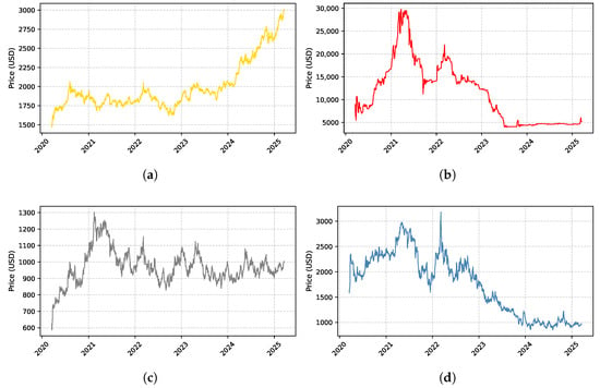
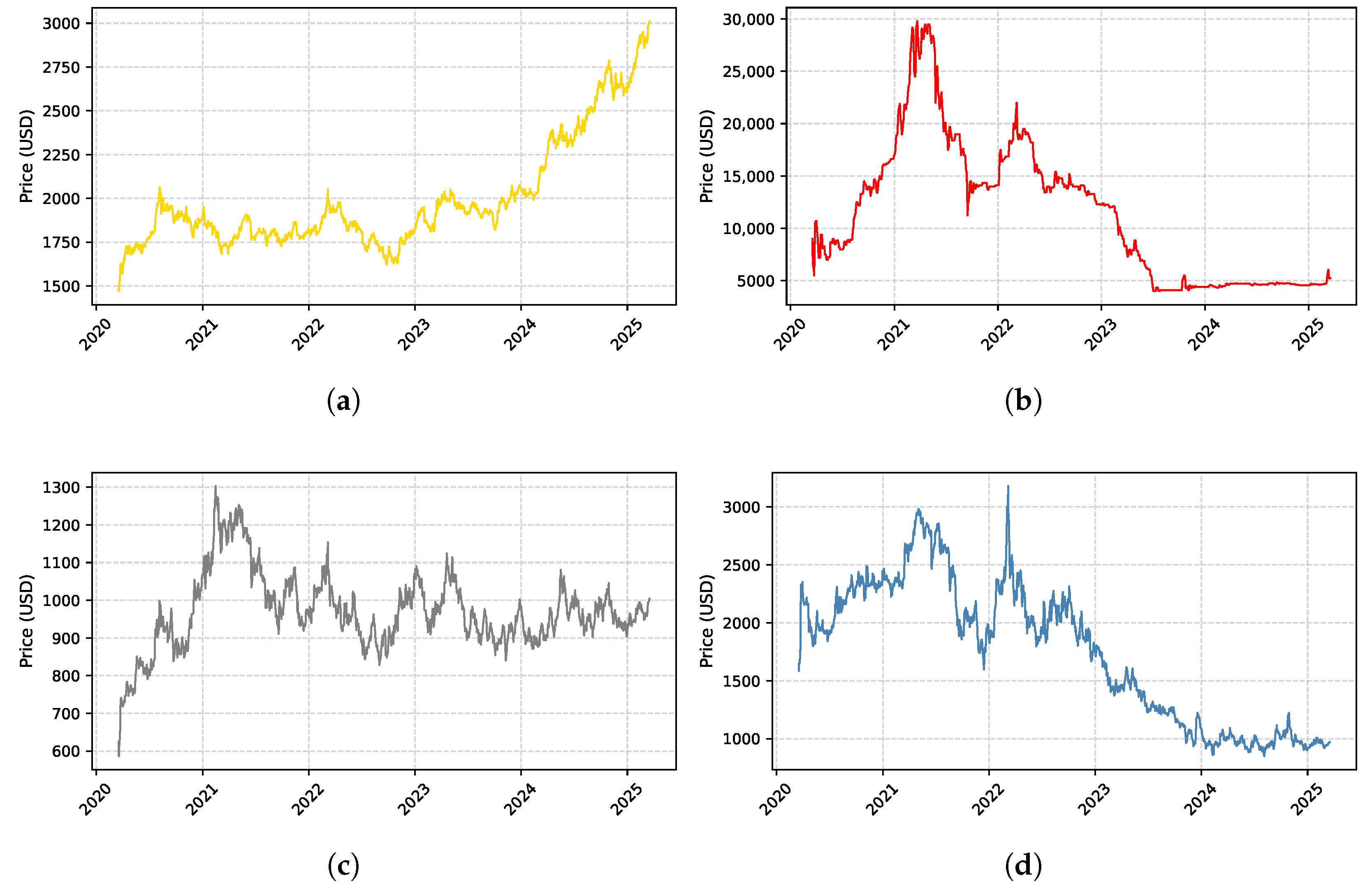
This study utilizes daily closing price data (in USD) for four precious metals, given in Figure 1. Specifically, the yellow line in subfigure (a) tracks Gold (XAU), the red line in subfigure (b) shows Rhodium (RHOD_LON), the grey line in subfigure (c) depicts Platinum (XPT) and the blue line in subfigure (d) represents Palladium (XPD), sourced from the JSE via Bloomberg. The dataset spans from 18 March 2020 to 18 March 2025, comprising 1299 observations.

Figure 1. The four time series plots are given as daily closing prices for: (a) Gold, (b) Rhodium, (c) Platinum and (d) Palladium.

2.2. Time Series Transformation

Logarithmic returns $r_t=ln\left(P_t\right)-ln\left(P_{t-1}\right)$ are computed, where $P_t$ and $P_{t-1}$ represent the closing prices at times t and $t-1$, respectively, to stabilize variance and ensure stationarity, a prerequisite for ARFIMA and FIGARCH modeling [10]. Stationarity of the log-return series is verified using the Augmented Dickey–Fuller (ADF) and Kwiatkowski–Phillips–Schmidt–Shin (KPSS) tests. The presence of conditional heteroskedasticity is confirmed via the Lagrange Multiplier (LM) test for ARCH effects.

The p-values, in Table 1, for the raw series and for the log-return are all below 0.05, indicating significant ARCH effects in the time series across all cases.

Table 1. ARCH LM test p-values for raw prices series and daily log-returns of precious metals.

Series	p-Value (Closing Prices)	p-Value (Log-Returns)
Gold	<$2.2\times {10}^{-16}$	$4.032\times {10}^{-6}$
Rhodium	<$2.2\times {10}^{-16}$	<$2.2\times {10}^{-16}$
Platinum	<$2.2\times {10}^{-16}$	$5.373\times {10}^{-11}$
Palladium	<$2.2\times {10}^{-16}$	$1.794\times {10}^{-6}$

2.3. Model Specification

To capture the dual stylized facts of persistent dependence in returns and long-memory persistence in volatility, we employ a unified fractionally integrated modeling framework utilizing the conditional mean ARFIMA(1,d,1) and conditional variance FIGARCH(1,d,1) processes. The ARFIMA(1,d,1) model is specified as $(1-{\varphi }_{1}L){(1-L)}^d{r}_t=(1+{\theta }_{1}L){ϵ}_t$, where ${\varphi }_1$ and ${\theta }_1$ are the autoregressive and moving average parameters, d is the fractional differencing parameter, and ${ϵ}_t\sim \mathcal{N}(0,{\sigma }^2)$ is white noise [4]. The fractional differencing parameter $d\in (-0.5,0.5)$ governs and captures long-memory effects in volatility [3]. To accommodate the slow, hyperbolic decay of volatility shocks observed across precious metal returns, the conditional variance ${\sigma }_t^2$ is specified through the FIGARCH(1,d,1) model as $[1-{\beta }_{1}L]{\sigma }_t^2=\omega +[1-(1-{\varphi }_{1}L){(1-L)}^d]{ϵ}_t^2$, where $\omega >0$ is the intercept, $d\in (0,1)$ parameterizes the fractional integration of volatility shocks, ${\beta }_1$ is the GARCH persistence parameter and ${\varphi }_1$ is the ARCH parameter of the model. The FIGARCH(1,d,1) model can be reparameterized in ARCH(∞) representation as ${\sigma }_t^2={\displaystyle \frac{\omega }{1-{\beta }_1}}+\lambda \left(L\right){ϵ}_t^2={\displaystyle \frac{\omega }{1-{\beta }_1}}+{\sum }_{k=1}^{\infty }{\lambda }_k{ϵ}_{t-k}^2$ where $\lambda \left(L\right)=1-{\displaystyle \frac{(1-{\varphi }_{1}L){(1-L)}^d}{1-{\beta }_{1}L}}$. To ensure strictly positive conditional variances (${\sigma }_t^2>0,\forall t$), the parameters must satisfy structural non-negativity inequality constraints: $\omega >0$, $0\le d\le 1-2{\varphi }_1$, and ${\beta }_1-d\le {\varphi }_1\le {\displaystyle \frac{2-d}{3}}$.

2.4. Optimization Methods

The estimation of ARFIMA and FIGARCH models relies on numerical optimization methods to maximize the log-likelihood function. We consider four algorithms widely used in econometrics and machine learning. The BFGS method is a quasi-Newton approach that approximates the Hessian matrix and provides robust convergence in many nonlinear problems [9]. The CG method is a first-order technique that requires little memory but often converges slowly or fails on ill-conditioned likelihood surfaces [11]. The L-BFGS algorithm extends BFGS by reducing memory requirements, making it suitable for higher-dimensional settings [9]. Finally, the Adam optimizer combines ideas from momentum and adaptive learning rates, and is particularly popular in machine learning applications for large datasets [12].

2.5. Model Evaluation Metrics

Parameter estimation is performed by maximizing the log-likelihood function, defined as $\mathcal{LL}(\Theta )=-{\displaystyle \frac{1}{2}}{\sum }_{t=1}^T\left(ln\left(2\pi \right)+ln\left({\sigma }_t^2\right)+{\displaystyle \frac{{ϵ}_t^2}{{\sigma }_t^2}}\right)$, where $\Theta$ is the parameter vector. Maximizing this log-likelihood function yields the optimum parameters, which are then used to evaluate and compare the efficiency of different numerical optimization methods, such as BFGS, CG, L-BFGS or Adam algorithms. In addition to the log-likelihood value, we also consider the number of iterations required for convergence. This metric provides insight into the computational efficiency and stability of each algorithm. While a higher log-likelihood indicates better fit, a smaller iteration count reflects faster convergence and reduced computational cost. Taken together, these measures give a clearer and more balanced view of both the accuracy and efficiency of the optimization methods.

2.6. Model Estimation and Performance Evaluation

Two long-memory models, ARFIMA(1,d,1) and FIGARCH(1,d,1), were fitted to the logarithmic return series of Gold, Rhodium, Platinum, and Palladium. Parameter estimation was carried out using several numerical optimization methods, namely BFGS, CG, L-BFGS, and Adam. The BFGS, CG, and L-BFGS approaches were implemented via the optim() function in R. For Adam, a custom implementation was developed to adapt the stochastic optimization framework with adaptive moments to the specific likelihood functions considered.

Four optimization algorithms were implemented to estimate model parameters. These were benchmarked against the R version 5.4.2 packages arfima and rugarch [13,14]. The analysis evaluates convergence stability, parameter consistency, and computational efficiency. To ensure fairness and avoid convergence to poor local optima, a principled and consistent initialization strategy was adopted, with starting values derived from OLS estimates. This approach aims to quantify parameter estimation risk and identify the most reliable optimization method for long-memory models [9].

To compare performance across methods, several evaluation metrics were used. The log-likelihood value served as a primary indicator of model fit, and the number of iterations required for convergence was considered as a practical measure of computational efficiency and stability.

Together, these criteria provide a comprehensive framework for assessing both the statistical accuracy and the practical feasibility of different optimization methods in estimating long-memory volatility models.

3. Results

3.1. ARFIMA Model Estimation

The estimation of the ARFIMA(1,d,1) model demonstrates remarkable stability across all optimization methods for the four precious metals. Table 2 presents the parameter estimates and log-likelihood values for Gold, Rhodium, Platinum and Palladium. The parameters ${\varphi }_1$, ${\theta }_1$, and d show minimal variation across BFGS, CG, L-BFGS, Adam and the arfima package, with log-likelihood values remaining nearly identical.

Table 2. In-sample parameter estimates, log-likelihood values and iteration counts for the ARFIMA(1,d,1) model across optimization methods.

Asset	Method	${\mathit{\varphi }}_1$	${\mathit{\theta }}_1$	d	Log-Likelihood	Iter
	BFGS	−0.4612	−0.5018	0.0310	6065.386	123
	CG	−0.4610	−0.5016	0.0310	6065.386	1693
Gold	L-BFGS	−0.4613	−0.5019	0.0309	6065.386	146
	Adam	−0.4596	−0.5003	0.0310	6065.386	432
	arfima	−0.4620	−0.5026	0.0310	6056.390	–
	BFGS	0.4934	−0.2796	0.1500	4993.194	12
	CG	0.4934	−0.2796	0.1500	4993.194	36
Rhodium	Adam	0.4933	−0.2799	0.1500	4993.194	146
	arfima	0.4934	−0.2797	0.1501	4993.190	–
	BFGS	0.3825	0.2351	0.1397	5261.868	13
	CG	0.3825	0.2351	0.1397	5261.868	640
Platinum	L-BFGS	0.3826	0.2352	0.1397	5261.868	23
	Adam	0.3825	0.2352	0.1397	5261.868	165
	arfima	0.3742	0.2295	0.1373	5261.870	–
	BFGS	0.4658	0.1865	0.1985	4792.083	13
	CG	0.4658	0.1865	0.1985	4792.083	292
Palladium	L-BFGS	0.4658	0.1865	0.1985	4792.083	19
	Adam	0.4651	0.1862	0.1981	4792.083	126
	arfima	0.4643	0.1861	0.1974	4792.080	–

The ARFIMA model demonstrates strong robustness across different optimization methods. Even though the estimation accuracy is consistent, the convergence speed varies. BFGS offers the best balance between stability and computational efficiency. The close results with the R package estimation support the validity of the implementation.

3.2. FIGARCH Model Estimation

In contrast, the FIGARCH(1,d,1) model exhibits significant sensitivity to the choice of optimization algorithm. Table 3 summarizes the results for all four metals, highlighting variations in parameter estimates ($\omega$, ${\varphi }_1$, ${\beta }_1$, d) and log-likelihood values. The FIGARCH model exhibits high sensitivity to the optimization algorithm. BFGS provides stable and interpretable estimates with reasonable computational effort. Adam often requires much more time to converge and may produce unstable estimates if not properly configured. L-BFGS sometimes leads to suboptimal solutions or fails to fully capture the model structure. The CG method performs poorly in this context, failing to converge for the majority of the financial series. Consequently, the parameter values for most metals under the FIGARCH model are omitted in the CG row, as the algorithm failed to satisfy the convergence criteria required for stable estimation. Its instability makes it less suitable for estimating FIGARCH models, which involve complex likelihood surfaces.

Table 3. In-sample parameter estimates, log-likelihood values, and iteration counts for the FIGARCH(1,d,1) model across optimization methods.

Asset	Method	$\mathit{\omega }(\times {10}^{-5})$	${\mathit{\varphi }}_1$	${\mathit{\beta }}_1$	d	Log-Likelihood	Iter
	BFGS	4.772	0.1240	0.0001	0.709	4129.49	154
	CG	-	-	-	-	-	-
Gold	L-BFGS	7.290	0.1983	0.0001	0.635	4102.93	92
	Adam	3.233	0.0707	0.0516	0.651	4135.01	398
	rugarch	0.097	0.0000	0.9216	0.999	4231.49	–
	BFGS	2.751	0.1524	0.0349	0.605	3564.08	211
	CG	-	-	-	-	-	-
Rhodium	L-BFGS	27.58	0.4797	0.0006	0.276	1897.08	113
	Adam	26.57	0.1356	0.0519	0.599	3564.03	2621
	rugarch	0.426	0.0000	-0.1684	0.431	3617.56	–
	BFGS	23.15	0.3037	0.0007	0.442	3287.03	123
	CG	23.90	0.2643	0.0006	0.491	3276.27	144
Platinum	L-BFGS	23.95	0.2632	0.0002	0.498	3290.08	118
	Adam	16.17	0.1464	0.0523	0.759	3341.88	2164
	rugarch	0.030	0.1149	0.9912	0.997	3437.11	–
	BFGS	53.33	0.1598	0.0008	0.327	2732.03	67
	CG	-	-	-	-	-	-
Palladium	L-BFGS	53.38	0.1609	0.0008	0.334	2726.43	66
	Adam	14.05	0.1749	0.0556	0.556	2920.49	7168
	rugarch	0.021	0.1730	0.9680	0.999	2984.97	–

Compared to the manual methods, the estimates obtained with the rugarch package differ significantly, especially for the long-memory parameter d, often producing values near the upper boundary.

3.3. Predictive Performance Evaluation

We evaluated the predictive performance of each optimization method using MSE and RMSE. It indicates how precise the models are in predicting future volatility.

Table 4 shows that both models achieve low MSE and RMSE values, indicating good forecasting performance. This suggests that ARFIMA(1,d,1) captures long-term return dynamics effectively, while FIGARCH provides a better fit for volatility clustering.

Table 4. In-sample predictive performance (MSE and RMSE) of the ARFIMA(1,d,1) and FIGARCH(1,d,1) models estimated using BFGS for the precious metals.

Series	MSE (ARFIMA)	MSE (FIGARCH)	RMSE (ARFIMA)	RMSE (FIGARCH)
Gold	$3.110\times {10}^{-8}$	$4.333\times {10}^{-8}$	0.000176	0.000208
Rhodium	$2.767\times {10}^{-6}$	$1.210\times {10}^{-5}$	0.001663	0.003479
Platinum	$3.283\times {10}^{-8}$	$3.832\times {10}^{-7}$	0.000181	0.000619
Palladium	$1.658\times {10}^{-7}$	$3.165\times {10}^{-6}$	0.000407	0.001779

BFGS appears to be the most robust and efficient optimization method for estimating both ARFIMA and FIGARCH models. It consistently produces stable parameter estimates, shows good results in residual diagnostics, and achieves good forecasting accuracy. These results support the use of BFGS in practical applications involving long-memory time series and volatility modeling.

4. Discussion

The results show a big difference in how stable the ARFIMA and FIGARCH models are when estimating parameters. For ARFIMA(1,d,1), the parameters are almost the same across all optimization methods. This consistency stems from utilizing the established “arfima” R package for likelihood evaluations. The package gives good starting values and uses tools like Fast Fourier Transform (FFT) to handle the calculations reliably [13]. Because of this, methods like BFGS, CG, L-BFGS, and Adam all find similar parameters. The main difference is speed. CG is slower and needs more iterations. We did not implement the likelihood function manually for ARFIMA, which keeps the results consistent. The model’s simple focus on long-memory in the mean also helps. However, studies show that estimation of the fractional parameter d can vary with different methods or software, explaining why consistency depends on reliable tools like the “arfima” package.

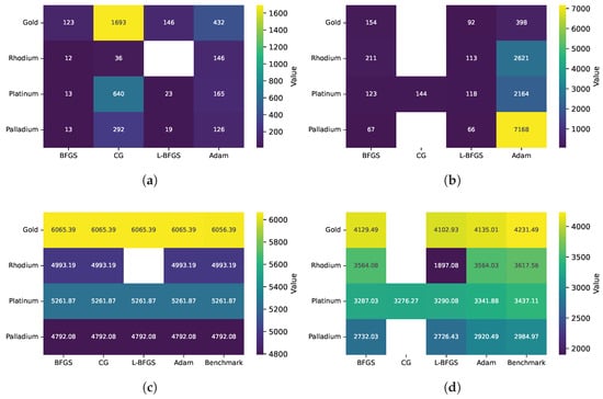
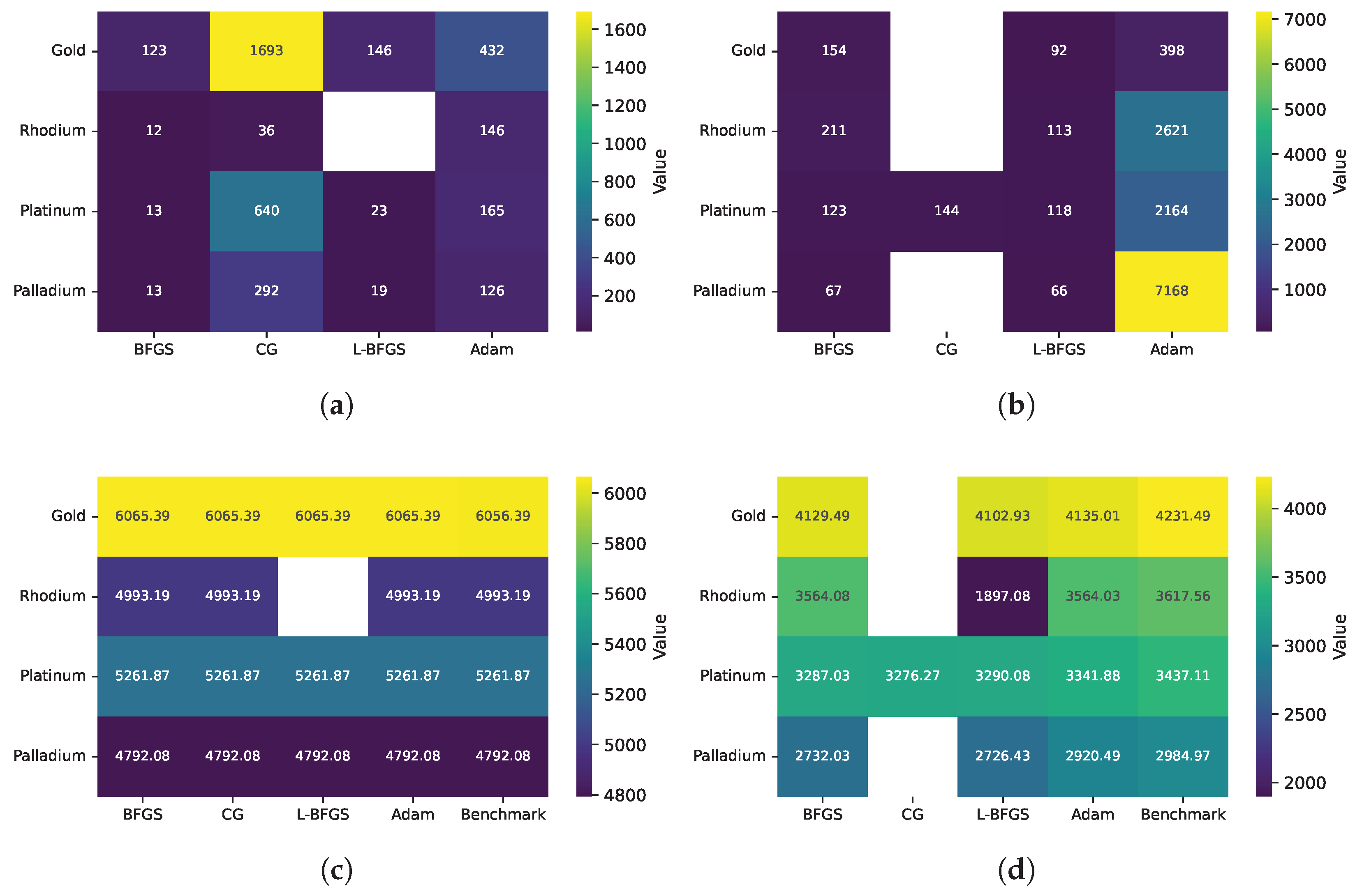
In contrast, FIGARCH(1,d,1) estimates exhibit substantial variability across optimizers due to the manual implementation of its highly non-convex likelihood surface. The fractional differencing parameter d and GARCH parameters (${\varphi }_1$, ${\beta }_1$) are closely linked, making optimization hard. BFGS works best because it uses second-order information to handle the tricky likelihood surface [9]. CG often fails to converge since it only uses first-order gradients, which is not enough for ill-conditioned problems like FIGARCH’s variance dynamics [15]. L-BFGS and Adam give inconsistent results, like the bad log-likelihood for Rhodium (−1897.08), because memory-efficient or adaptive methods struggle with high-dimensional spaces in complex models [16]. Compared to our manual methods, the rugarch package gives different estimates, often with d close to 1, because of its internal rules. The differences with rugarch estimates (e.g., $d\approx 1$) come from software choices, adding more risk. This needs more study. Overall, choosing the right optimizer is important for good volatility modeling in precious metals markets. Figure 2a–d show the heatmaps of log-likelihoods and iteration counts for ARFIMA(1,d,1) and FIGARCH(1,d,1) models across different precious metals and optimization methods. White or empty cells indicate failed convergence or unavailable iteration data.

Figure 2. The iteration counts for the two models are presented in the (a) iterations for ARFIMA(1,d,1) and (b) iterations for FIGARCH(1,d,1). The log-likelihood values for the two models are revealed in the (c) log-likelihood for ARFIMA(1,d,1) and (d) log-likelihood for FIGARCH(1,d,1).

5. Out-of-Sample Validation

In time series analysis, obtaining high-quality in-sample results is a necessary but insufficient condition for comprehensive model validation. To demonstrate that the goodness of fit and the quality of parameter estimation are not products of overfitting or numerical artifacts, it is crucial to perform an out-of-sample validation. Assessing the reliability of estimated parameters on unseen data is fundamental for practical risk management and financial forecasting. In this section, we evaluate the predictive performance of the previously estimated parameters of ARFIMA and FIGARCH models using an independent dataset.

5.1. Data and Methodology

The validation dataset consists of 325 daily observations for Gold, Rhodium, Platinum, and Palladium, spanning from 1 January 2025 to 31 March 2026. This period remains independent of the in-sample data used for initial model fitting. To ensure consistency with the modeling requirements and stabilize the variance, the raw price series were transformed into daily log-returns. Unlike the estimation phase, the out-of-sample validation employs the fixed parameters obtained in Table 2 and Table 3. The forecasting performance of the ARFIMA(1,d,1) and FIGARCH(1,d,1) models was evaluated using four key metrics: Mean Squared Error (MSE), Root Mean Squared Error (RMSE), Mean Absolute Error (MAE), and log-likelihood.

5.2. Analysis of Results

Table 5 and Table 6 show the results of the validation. For the ARFIMA(1,d,1) model, the predictive performance remained remarkably consistent across all optimizers, with MSE and RMSE values showing minimal variance. This consistency is attributed to the use of the arfima package in R, which provides a highly stable environment for computing the likelihood function.

Table 5. Out-of-sample predictive performance metrics (MSE, RMSE, MAE, and log-likelihood) for the ARFIMA(1,d,1) model across optimization methods.

Asset	Method	MSE	RMSE	MAE	Log-Likelihood
Gold	BFGS	0.00023	0.01532	0.01057	1353.932
	CG	0.00023	0.01532	0.01057	1353.932
	L-BFGS	0.00023	0.01532	0.01057	1353.936
	Adam	0.00023	0.01532	0.01057	1353.932
	arfima package	0.00023	0.01531	0.01054	1357.368
Rhodium	BFGS	0.00030	0.01737	0.01045	1318.517
	CG	0.00030	0.01737	0.01045	1318.517
	Adam	0.00030	0.01737	0.01045	1318.497
	arfima package	0.00030	0.01718	0.01074	1351.799
Platinum	BFGS	0.00077	0.02776	0.01794	1141.201
	CG	0.00077	0.02776	0.01794	1141.201
	L-BFGS	0.00077	0.02776	0.01794	1141.201
	Adam	0.00077	0.02776	0.01794	1141.211
	arfima package	0.00077	0.02778	0.01798	1161.978
Palladium	BFGS	0.00074	0.02723	0.01808	1118.244
	CG	0.00074	0.02723	0.01808	1118.244
	L-BFGS	0.00074	0.02723	0.01808	1118.244
	Adam	0.00074	0.02723	0.01808	1118.360
	arfima package	0.00074	0.02721	0.01804	1171.429

Table 6. Out-of-sample predictive performance metrics (MSE, RMSE, MAE, and log-likelihood) for the FIGARCH(1,d,1) model across optimization methods.

Asset	Method	MSE	RMSE	MAE	Log-Likelihood
Gold	BFGS	0.00024	0.01547	0.01072	902.694
	L-BFGS	0.00024	0.01546	0.01072	900.820
	Adam	0.00024	0.01546	0.01072	911.246
	rugarch package	0.00024	0.01541	0.01072	946.504
Rhodium	BFGS	0.00030	0.01728	0.00991	859.287
	L-BFGS	0.00030	0.01723	0.01000	−12,750.473
	Adam	0.00030	0.01725	0.01000	838.685
	rugarch package	0.00030	0.01729	0.00988	934.705
Platinum	BFGS	0.00078	0.02796	0.01803	750.060
	CG	0.00078	0.02796	0.01803	750.065
	L-BFGS	0.00078	0.02796	0.01803	750.066
	Adam	0.00078	0.02795	0.01805	734.568
	rugarch package	0.00078	0.02788	0.01807	779.100
Palladium	BFGS	0.00076	0.02765	0.01818	689.968
	L-BFGS	0.00076	0.02765	0.01818	690.866
	Adam	0.00076	0.02760	0.01815	730.577
	rugarch package	0.00074	0.02729	0.01801	753.850

In contrast, for the FIGARCH(1,d,1) model, the sensitivity observed in-sample persisted in the validation phase. Due to the manual implementation of the FIGARCH likelihood function, the choice of the optimizer played a critical role. The BFGS algorithm consistently achieved the most robust results, providing stable updates even for the most volatile series. While methods like Adam and L-BFGS may occasionally yield higher log-likelihood scores on specific assets, they demonstrate inconsistency and convergence failures, reinforcing the conclusion that second-order optimization for BFGS is essential for the complex likelihood surfaces of long-memory volatility models.

6. Conclusions

This study provides a comprehensive evaluation of parameter estimation risk in ARFIMA(1,d,1) and FIGARCH(1,d,1) models applied to daily log-returns of four precious metals, namely Gold, Rhodium, Platinum, and Palladium, sourced from the JSE over the period from 18 March 2020 to 18 March 2025. Our findings reveal a clear difference in estimation stability: the ARFIMA model shows robust convergence across optimization methods, including BFGS, CG, L-BFGS, Adam and the arfima package, with minimal estimation risk. This stability stems from the arfima package’s reliable likelihood computation and internal setting, though convergence speed varies: CG is notably slower. In contrast, the FIGARCH model exhibits significant sensitivity to the choice of optimizer, with BFGS providing the most stable and reliable estimates, while CG often fails to converge, and L-BFGS and Adam yield inconsistent results.

Crucially, the out-of-sample validation phase conducted on an independent dataset from January 2025 to March 2026 using fixed parameters corroborates these findings. By applying the previously estimated parameters directly to the log-returns of unseen price data, we confirmed that the predictive performance and model stability are intrinsically linked to the initial optimization quality. Even in instances where adaptive methods like Adam occasionally achieved higher local log-likelihood values, they exhibited significant numerical instability compared to second-order approaches. Our findings confirm that the superiority of the BFGS algorithm stems from its use of Hessian-based information, which provides a more robust curvature approximation than the momentum-based updates of Adam, ensuring more reliable convergence in the presence of long-memory parameters. Consequently, robust quasi-Newton methods should be prioritized in practice to ensure accurate and stable volatility forecasts.

These results underscore the critical role of optimization method selection in long-memory volatility modeling, particularly for complex models like FIGARCH. The observed variability in parameter estimates, especially for volatile assets like Rhodium, highlights a potential source of model risk that could impact financial decision-making, such as risk assessment and portfolio optimization [2].

Limitations of this study include the focus on a specific model specification (1,d,1) and a single dataset, which may not generalize to other financial assets or time periods. Future research could explore higher-order ARFIMA and FIGARCH variants, such as FIAPARCH or HYGARCH, and extend the analysis to diverse markets or higher-frequency data [17]. Additionally, incorporating advanced optimization techniques, such as stochastic gradient methods, could further refine estimation accuracy. These directions would enhance the robustness and applicability of long-memory models in financial econometrics.

References

- Cont, R. Empirical Properties of Asset Returns: Stylized Facts and Statistical Issues. Quant. Financ. 2001, 1, 223–236. [Google Scholar] [CrossRef] [Scilit]
- Glasserman, P.; Xu, X. Robust Risk Measurement and Model Risk. Quant. Financ. 2014, 14, 29–58. [Google Scholar] [CrossRef] [Scilit]
- Baillie, R.T.; Bollerslev, T.; Mikkelsen, H.O. Fractionally Integrated Generalized Autoregressive Conditional Heteroskedasticity. J. Econom. 1996, 74, 3–30. [Google Scholar] [CrossRef] [Scilit]
- Granger, C.W.J.; Joyeux, R. An Introduction to Long-Memory Time Series Models and Fractional Differencing. J. Time Ser. Anal. 1980, 1, 15–29. [Google Scholar] [CrossRef] [Scilit]
- Bollerslev, T. Generalized Autoregressive Conditional Heteroskedasticity. J. Econom. 1986, 31, 307–327. [Google Scholar] [CrossRef] [Scilit]
- Boateng, A.; Gil-Alana, L.; Siweya, H.; Belete, A. Long Memory and ARFIMA Modelling: The Case of CPI Inflation Rate in Ghana. J. Dev. Areas 2016, 50, 287–304. [Google Scholar] [CrossRef] [Scilit]
- Beran, J. Maximum Likelihood Estimation of the Differencing Parameter for Invertible Short and Long Memory Autoregressive Integrated Moving Average Models. J. R. Stat. Soc. Ser. B Methodol. 1995, 57, 659–672. [Google Scholar] [CrossRef] [Scilit]
- Seitshiro, M.B.; Mashele, H.P. Assessment of Model Risk due to the use of an Inappropriate Parameter Estimator. Cogent Econ. Financ. 2020, 8, 1710970. [Google Scholar] [CrossRef] [Scilit]
- Nocedal, J.; Wright, S.J. Numerical Optimization, 2nd ed.; Springer: New York, NY, USA, 2006. [Google Scholar]
- Hamilton, J.D. Time Series Analysis; Princeton University Press: Princeton, NJ, USA, 1994. [Google Scholar]
- Hestenes, M.R.; Stiefel, E. Methods of Conjugate Gradients for Solving Linear Systems. J. Res. Natl. Bur. Stand. 1952, 49, 409–436. [Google Scholar] [CrossRef] [Scilit]
- Kingma, D.P.; Ba, J. Adam: A Method for Stochastic Optimization. In Proceedings of the International Conference on Learning Representations (ICLR), San Diego, CA, USA, 7–9 May 2015. [Google Scholar]
- Veenstra, J.Q.; McLeod, A.I. The arfima Package: ARFIMA Models in R. J. Stat. Softw. 2015, 66, 1–36. [Google Scholar]
- Ghalanos, A. rugarch: Univariate GARCH Models. 2020. Available online: https://cran.r-project.org/web/packages/rugarch/index.html (accessed on 24 May 2025).
- Tayefi, M.; Ramanathan, T.V. An overview of FIGARCH and related time series models. Int. J. Econ. Financ 2012, 4, 97–110. [Google Scholar] [CrossRef] [Scilit]
- Brunetti, C.; Gilbert, C.L. Bivariate FIGARCH and Fractional Cointegration. J. Empir. Financ. 2000, 7, 509–530. [Google Scholar] [CrossRef] [Scilit]
- Khumalo, M.; Mashele, H.; Seitshiro, M. Quantification of the Stock Market Value at Risk by using FIAPARCH, HYGARCH and FIGARCH Models. Data Sci. Financ. Econ. 2023, 3, 380–400. [Google Scholar] [CrossRef] [Scilit]
Disclaimer/Publisher’s Note: The statements, opinions and data contained in all publications are solely those of the individual author(s) and contributor(s) and not of MDPI and/or the editor(s). MDPI and/or the editor(s) disclaim responsibility for any injury to people or property resulting from any ideas, methods, instructions or products referred to in the content. |
© 2026 by the authors. Licensee MDPI, Basel, Switzerland. This article is an open access article distributed under the terms and conditions of the Creative Commons Attribution (CC BY) license.