A Simulation Study of Stabilized Logistic Predictions Under Separation ^†

Abstract

Logistic regression is widely used for binary risk prediction, but complete or quasi-separation can make maximum-likelihood fitting unstable and drive coefficients and fitted probabilities to extreme values. We present a stabilization idea based on suppressing weak-curvature directions in the local likelihood geometry and estimating only on the stable subspace. Using a simple exact-separation example and repeated train/test simulations with perturbed test sets, we show that stabilization yields less saturated probability estimates and substantially improves out-of-sample prediction once the test setting departs from exact separation.

1. Introduction

Logistic regression remains a standard tool for binary risk modeling, but in sparse or highly imbalanced data is vulnerable to complete or quasi-separation. It is known that in this case, maximum-likelihood estimates may diverge even when in-sample classification appears nearly perfect; see [1,2,3] as well as [4]. Separation is especially relevant when the binary response records whether an event occurs within a follow-up window or fixed period. Examples include adverse events during clinical-trial follow-up, onset of disease within a given time horizon in epidemiologic studies, severe car crashes at a location over a specified period, and customer churn or return purchasing after an advertising campaign [5,6,7]. In such settings the practical target is usually not perfect retrospective classification, but a stable probability model that can be transported to the next sample. This paper is intentionally narrow. We use a geometric stabilization idea to argue that when the likelihood becomes nearly singular, one should estimate and predict only in directions supported by adequate local information. The goal is a short applied note showing why ordinary logistic fits can look excellent under exact separation and yet behave poorly under mild perturbation, while stabilized fitting yields more credible probabilities and more robust predictive summaries. The motivating applied picture is therefore predictive rather than purely geometric. A strong biomarker, a screening rule, a road feature, or a high-intent customer signal may nearly determine the observed outcome in a small sample, but that does not guarantee that the fitted probabilities remain useful when the next cohort, road period, or advertising campaign is slightly different. This predictive perspective guides both the example and the simulation design.

2. Separation and Stabilization

Separation occurs when a linear combination of the predictors perfectly classifies events and non-events, or does so up to ties. The existence of the logistic MLE depends on the geometric configuration of data, as established by [1]. Under separation, some coefficients diverge and the corresponding fitted probabilities approach 0 or 1. For prediction, this creates a trap. On the same (or a nearly identical) separated sample, a standard logistic fit can achieve excellent scores because extreme probabilities are rewarded when the labels follow the same separating rule. Yet the fitted model is brittle: small covariate perturbations, small label noise, or modest departures from the exact separating geometry can lead to much larger losses. The central distinction in this paper is therefore between apparent success on an exactly separated sample and robust predictive performance under repeated resampling and perturbed test settings. Let $\ell \left(\beta \right)$ be the logistic log-likelihood, $U\left(\beta \right)$ its score, and $I\left(\beta \right)$ the local information matrix. In regular regimes, Newton or Fisher scoring updates $\beta$ by applying $I{\left(\beta \right)}^{-1}$ to the score. Under separation or near-separation, however, $I\left(\beta \right)$ becomes poorly conditioned and the update can be dominated by directions with little curvature support. Our stabilization device is deliberately simple. Writing the eigendecomposition

$$I\left(\beta \right)=V\mathrm{\Lambda }{V}^{\top },$$

we identify a stable subset of eigendirections and suppress the unstable ones. Moreover, let $\mathrm{\Lambda }=diag({\lambda }_1,\dots ,{\lambda }_p)$, with ${\lambda }_{max}={max}_j\left\{{\lambda }_j\right\}$. We define the stable subspace through the data-driven floor

$$\epsilon =max\{{\epsilon }_{\mathrm{num}},\tau {\lambda }_{max}/n\},\tau >0,$$

where ${\epsilon }_{\mathrm{num}}$ is a small numerical safeguard and $\tau$ is a tuning constant. The stable subspace is then the span of eigenvectors whose eigenvalues satisfy ${\lambda }_j\ge \epsilon$. Equivalently, we have ${\lambda }_j/{\lambda }_{max}\ge \tau /n$, while the complementary directions are treated as locally weakly identified and are not followed by the update. In practice, the stabilized step is obtained by projecting the score onto this stable subspace, so that directions with sufficiently strong curvature are retained and directions with collapsing curvature are suppressed. This changes not only the direction of the update but also its effective size, because removing unstable score components typically shortens the step and yields more conservative movement near separation. The rule is scale-adaptive, also works in very low dimensions, and reduces to ordinary logistic regression when all eigenvalues remain well above the threshold. In the experiments below we use $\tau =0.3$ as a practical default, with qualitatively similar behavior over the range $\tau \in [0.2,0.8]$. If $V_S$ and ${\mathrm{\Lambda }}_S$ denote the eigenvectors and eigenvalues associated with the stable directions, and if $U_S\left(\beta \right)=V_S{V}_S^{\top }U\left(\beta \right)$ is the score projected onto the stable subspace, the stabilized update is

$$\Delta {\beta }_{\mathrm{stab}}=V_S{\mathrm{\Lambda }}_S^{-1}{V}_S^{\top }U\left(\beta \right)=V_S{\mathrm{\Lambda }}_S^{-1}{V}_S^{\top }{U}_S\left(\beta \right).$$

Thus only the score components supported by adequate local curvature contribute to the update, while score components in unstable directions are discarded rather than amplified. This affects both the direction and the effective size of the step, since removing unstable components typically yields a shorter and more conservative move near separation. Therefore, when separation destroys effective curvature, estimation proceeds on the stable subspace only. If the ordinary MLE exists, the stabilized fit remains close to it; if the ordinary MLE does not exist, the same construction still yields a finite pseudo-solution and hence finite fitted probabilities. This viewpoint is intentionally geometric rather than fully penalized or prior-based. The problem is not merely that coefficients are large; it is that some local directions are effectively unsupported by curvature and so should not be allowed to dominate the update. It is also worth noting that while separation in logistic regression is usually addressed through penalization or bias reduction [4], the present construction is also related, at a numerical level, to projected and iterative regularization for ill-posed problems, where updates are stabilized by restricting attention to well-supported directions [8].

3. Why Stabilization Helps Prediction

In exact separation, a conventional logistic fit can produce huge coefficients and nearly perfect classification on the same separating geometry. That does not make it a good probability model; it means only that the fitted logits are so extreme that the implied probabilities are practically binary. A stabilized fit targets a different object: a finite probability map supported by the informative part of the local geometry. Accordingly, we evaluate the methods not only by discrimination but also by proper scoring rules and direct summaries of saturation and instability [9,10,11,12]. For binary outcomes $y_i\in \{0,1\}$ with predicted probabilities $p_i$, the log-loss is

$$\mathrm{LogLoss}=-{\displaystyle \frac{1}{n}}{\displaystyle \sum _{i=1}^n}\left\{y_{i}log{p}_i+(1-y_i)log(1-p_i)\right\},$$

so smaller values indicate better calibrated and less overconfident probabilities. The Brier score is

$$\mathrm{Brier}={\displaystyle \frac{1}{n}}{\displaystyle \sum _{i=1}^n}{(y_i-p_i)}^2,$$

and again smaller is better. The AUC is defined empirically as

$$\mathrm{AUC}={\displaystyle \frac{1}{n_1{n}_0}}\sum _{i:Y_i=1}\sum _{j:Y_j=0}\left[\mathbf{1}\{{\widehat{p}}_i>{\widehat{p}}_j\}+{\displaystyle \frac{1}{2}}\mathbf{1}\{{\widehat{p}}_i={\widehat{p}}_j\}\right],$$

where $n_1={\sum }_i\mathbf{1}\{Y_i=1\}$ and $n_0={\sum }_i\mathbf{1}\{Y_i=0\}$ denote the numbers of events and non-events, respectively. The AUC can be interpreted as the probability that a randomly chosen event receives a higher score than a randomly chosen non-event, so larger values indicate better discrimination. The distinction between ranking and probability estimation is important for the results that follow. Under exact separation, both standard and stabilized fits can rank observations almost perfectly, so AUC alone cannot diagnose the pathology. Proper scoring rules are more informative because they penalize overconfident wrong predictions once the test set departs from the training geometry. The saturation summaries then explain why one method deteriorates faster than the other.

4. A Simple Exact-Separation Simulation Example

We consider the stylized example

$$Y_i=\mathbf{1}(X_i>0),X_i\sim N(0,1),$$

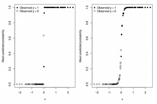
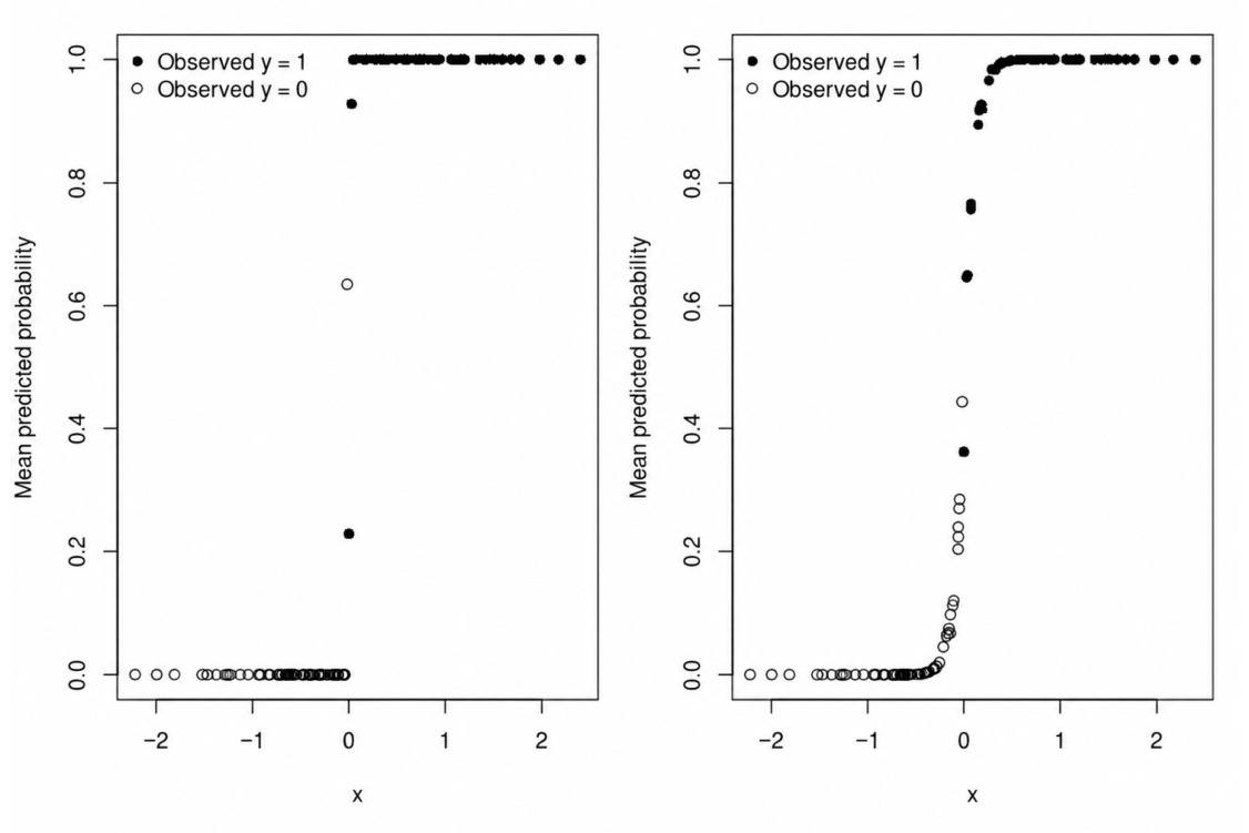
which yields exact separation by construction. The example is intentionally simple: it isolates the geometry of separation and makes the predictive consequences visible. In this design, the classical logistic fit drives the slope toward very large values and produces fitted probabilities essentially equal to 0 or 1, whereas the stabilized fit remains finite and retains a wider transition zone; see Figure 1. We therefore interpret the stabilized curve not as automatically being more accurate from the plot alone, but as less saturated and more credible as a probability model under separation.

Figure 1. Predicted probabilities in the exact-separation example, averaged over repeated resamples. The conventional fit (left panel) collapses toward near-binary probabilities, whereas the stabilized fit (right panel) preserves a wider transition zone. Filled points denote events and open points denote non-events.

In our simulations we use repeated 70%/30% train/test resampling from the exact-separation design with a total of $n=120$ observations. Two benchmark scenarios are reported throughout: exact separation on both training and test sets, and perturbed test sets in which the training split is unchanged but the test side is modified by added noise and/or label flips. Each benchmark uses 50 resamples. We also run a 12-scenario suite combining test-noise levels 0, $0.1$, $0.25$, and $0.5$ with label-flip rates 0, $0.02$, and $0.05$. Here noise denotes the standard deviation of an independent Gaussian perturbation added to the test covariate and flip denotes the probability of independently reversing the binary test label. The main metrics are mean log-loss, mean Brier score, and mean AUC, interpreted as defined in Section 3, together with coefficient and saturation summaries. We do not emphasize response-scale interval coverage for Bernoulli outcomes, because it concerns the mean probability rather than the realized $0/1$ outcome and can be misleading in separated settings.

5. Simulation Results

Table 1 shows that in exact separation, both methods attain an AUC equal to one, so discrimination is not the relevant distinction. The stabilized fit has slightly lower mean log-loss (0.0539 versus 0.0637), whereas the conventional fit has a slightly better mean Brier score (0.0129 versus 0.0150).

Table 1. Benchmark repeated-split summaries for the exact-separation and perturbed test scenarios (50 resamples). Lower log-loss and Brier are better; higher AUC is better.

Scenario	Method	Log-Loss	Brier	AUC
Exact	Standard logistic	0.0637	0.0129	1.0000
Exact	Stabilized logistic	0.0539	0.0150	1.0000
Perturbed	Standard logistic	2.3573	0.0912	0.9171
Perturbed	Stabilized logistic	0.8433	0.0779	0.9541

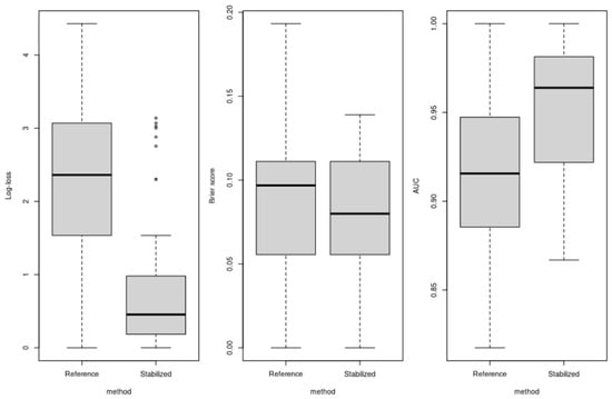
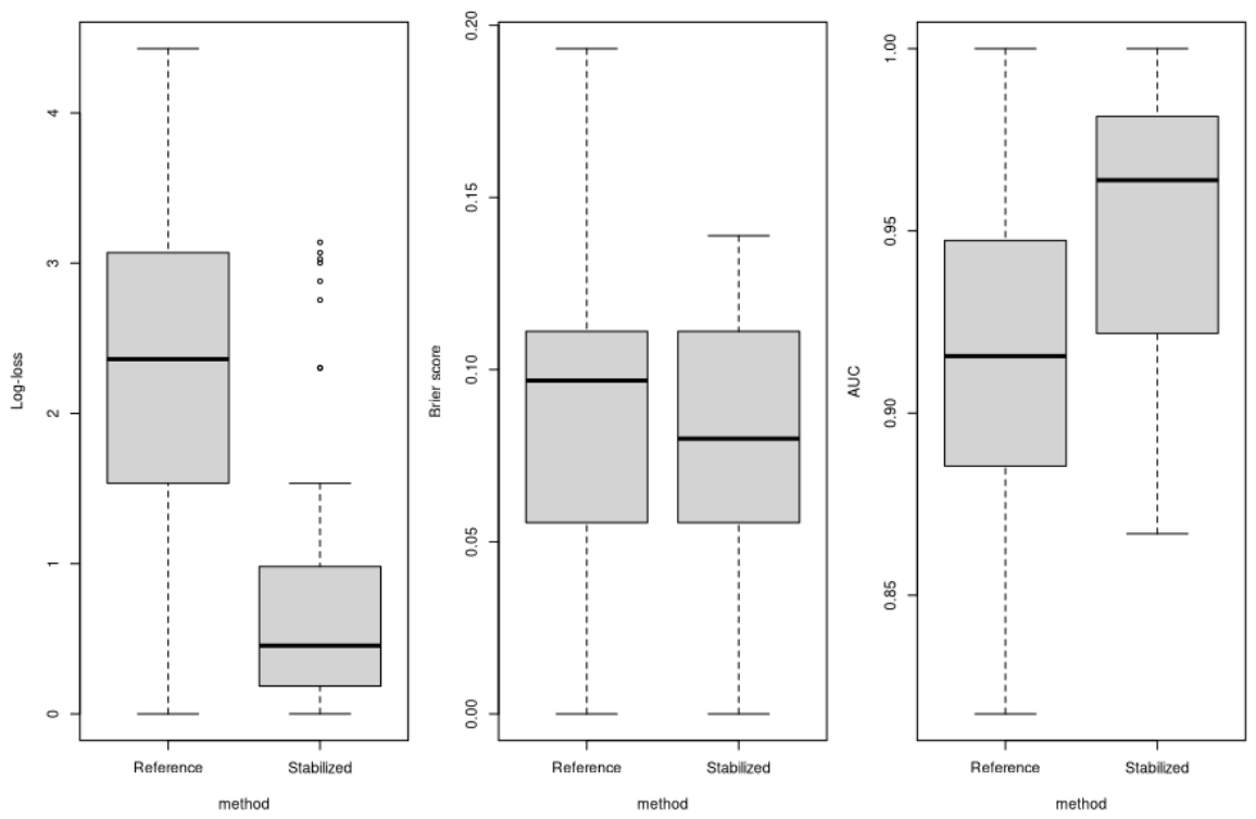
The stabilized fit has a slightly lower mean log-loss (0.0539 versus 0.0637), whereas the conventional fit has a slightly better mean Brier score (0.0129 versus 0.0150). This is the expected ambiguous regime: if the test set follows the same separating rule, extreme probabilities are rewarded. The stability summaries are more informative. The conventional fit shows severe coefficient inflation, whereas the stabilized fit remains much smaller and more stable across resamples. Figure 1 shows the same point graphically: the conventional fit collapses toward the poles and leaves almost no probability mass in the interior, whereas the stabilized fit is distinctly less saturated. Once the test set is perturbed, the advantage of stabilization becomes clear. In the benchmark perturbed test scenario of Table 1, the stabilized fit improves all three principal summaries: mean log-loss drops from 2.3573 to 0.8433, mean Brier score drops from 0.0912 to 0.0779, and mean AUC rises from 0.9171 to 0.9541. The boxplots in Figure 2 show the same uniform shift.

Figure 2. Resampling distributions of log-loss (left panel), Brier score (central panel), and AUC (right panel) under perturbed testing. The stabilized fit dominates on all three metrics.

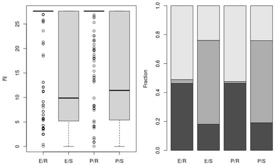
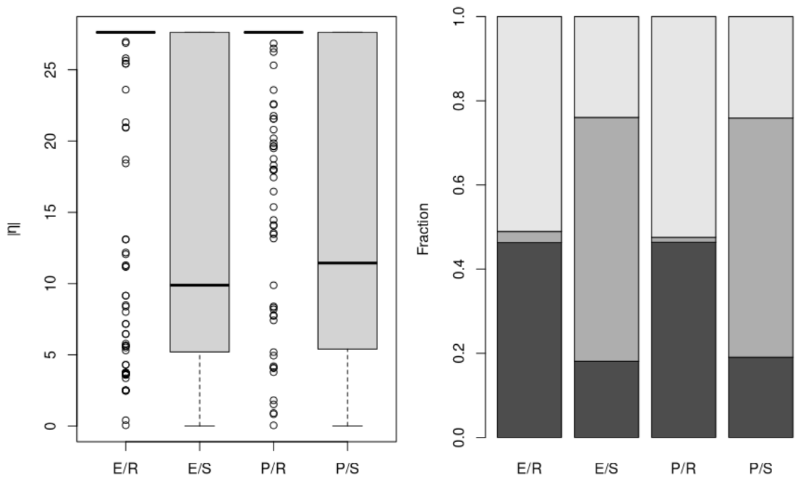
This is the main empirical message of the paper: the conventional fit appears strongest only when the test geometry preserves exact separation, whereas the stabilized fit behaves like a more robust probability model once that geometry is weakened. The broader 12-scenario suite confirms the same pattern. Table 2 reports the mean resampled log-loss and mean AUC for all combinations of test noise and label-flip rates; lower log-loss and higher AUC indicate better predictive performance. As perturbation increases, the conventional fit deteriorates much faster. With zero label flips, for example, mean log-loss rises from 0.0637 to 4.1508, while the corresponding stabilized values rise only from 0.0539 to 1.4329. AUC also increasingly favors stabilization. Figure 3 provides the matching saturation diagnostics. The conventional fit remains highly saturated, while the stabilized fit keeps a much larger proportion of probabilities away from the extremes. Because the perturbation is applied on the test side, these differences reflect how the fitted models react to departures from exact separation rather than a change in the fitted training coefficients.

Table 2. Full perturbation suite. Noise is the test-side covariate perturbation and flip is the test-side label-flip rate. Lower log-loss is better; higher AUC is better.

Noise	Flip	LLstd	AUCstd	LLstab	AUCstab
0	0	0.0637	1.0000	0.0539	1.0000
0	0.02	0.5875	0.9820	0.3052	0.9819
0	0.05	1.2557	0.9579	0.6454	0.9573
0.10	0	0.8663	0.9728	0.2028	0.9945
0.10	0.02	1.3950	0.9529	0.5143	0.9751
0.10	0.05	2.0348	0.9294	0.8913	0.9484
0.25	0	1.9395	0.9332	0.5710	0.9718
0.25	0.02	2.3573	0.9171	0.8433	0.9541
0.25	0.05	2.9239	0.8965	1.2014	0.9287
0.50	0	4.1508	0.8512	1.4329	0.9178
0.50	0.02	4.4885	0.8391	1.6815	0.9020
0.50	0.05	4.9644	0.8222	1.9982	0.8797

Figure 3. Saturation diagnostics for logistic regression. The left panel summarizes the linear predictor and the right panel the distribution of fitted probabilities across the bands Near 0 (light gray), Interior (medium gray), and Near 1 (dark gray). E/R = Exact/standard fit, E/S = exact/stabilized fit, P/R = perturbed/standard fit, P/S = perturbed/stabilized fit. The stabilized fit is less saturated in all settings.

6. Discussion

The main message of this paper is simple. In separated logistic problems, the ordinary MLE can look excellent when the test data preserve the same separating geometry, but that success is driven by saturated probabilities and coefficient inflation rather than by robust probability estimation. Under repeated resampling and perturbed test sets, the stabilized fit behaves much more favorably.

This matters for applications because binary event indicators over fixed periods are common in clinical prediction, epidemiology, traffic safety, and conversion modeling. It also means that predictive summaries should be read together with stability diagnostics. In exact separation, AUC is largely uninformative because both methods can rank perfectly, and the Brier score may even modestly favor the saturated fit. Once the test geometry is perturbed, however, the proper scoring rules become decisive and favor the stabilized fit. The running example is stylized and the perturbations are generic, but they are enough to show that stabilization produces a more finite, less saturated, and more reliable probability model.

References

- Albert, A.; Anderson, J.A. On the existence of maximum likelihood estimates in logistic regression models. Biometrika 1984, 71, 1–10. [Google Scholar] [CrossRef] [Scilit]
- Heinze, G.; Schemper, M. A solution to the problem of separation in logistic regression. Stat. Med. 2002, 21, 2409–2419. [Google Scholar] [CrossRef] [Scilit] [PubMed]
- King, G.; Zeng, L. Logistic regression in rare events data. Political Anal. 2001, 9, 137–163. [Google Scholar] [CrossRef] [Scilit]
- Mansournia, M.A.; Geroldinger, A.; Greenland, S.; Heinze, G. Separation in logistic regression: Causes, consequences, and control. Am. J. Epidemiol. 2018, 187, 864–870. [Google Scholar] [CrossRef] [Scilit] [PubMed]
- Al-Ghamdi, A.S. Using logistic regression to estimate the influence of accident factors on accident severity. Accid. Anal. Prev. 2002, 34, 729–741. [Google Scholar] [CrossRef] [Scilit] [PubMed]
- Neslin, S.A.; Gupta, S.; Kamakura, W.; Lu, J.; Mason, C.H. Defection detection: Measuring and understanding the predictive accuracy of customer churn models. J. Mark. Res. 2006, 43, 204–211. [Google Scholar] [CrossRef] [Scilit]
- Shipe, M.E.; Deppen, S.A.; Farjah, F.; Grogan, E.L. Developing prediction models for clinical use using logistic regression: An overview. J. Thorac. Dis. 2019, 11, S574–S584. [Google Scholar] [CrossRef] [Scilit] [PubMed]
- Kilmer, M.E.; O’Leary, D.P. Choosing regularization parameters in iterative methods for ill-posed problems. SIAM J. Matrix Anal. Appl. 2001, 22, 1204–1221. [Google Scholar] [CrossRef] [Scilit]
- Brier, G.W. Verification of forecasts expressed in terms of probability. Mon. Weather. Rev. 1950, 78, 1–3. [Google Scholar]
- Gneiting, T.; Raftery, A.E. Strictly proper scoring rules, prediction, and estimation. J. Am. Stat. Assoc. 2007, 102, 359–378. [Google Scholar] [CrossRef] [Scilit]
- Hanley, J.A.; McNeil, B.J. The meaning and use of the area under a receiver operating characteristic curve. Radiology 1982, 143, 29–36. [Google Scholar] [CrossRef] [Scilit] [PubMed]
- Steyerberg, E.W.; Vickers, A.J.; Cook, N.R.; Gerds, T.; Gonen, M.; Obuchowski, N.; Pencina, M.J.; Kattan, M.W. Assessing the performance of prediction models: A framework for traditional and novel measures. Epidemiology 2010, 21, 128–138. [Google Scholar] [PubMed]
Disclaimer/Publisher’s Note: The statements, opinions and data contained in all publications are solely those of the individual author(s) and contributor(s) and not of MDPI and/or the editor(s). MDPI and/or the editor(s) disclaim responsibility for any injury to people or property resulting from any ideas, methods, instructions or products referred to in the content. |
© 2026 by the author. Licensee MDPI, Basel, Switzerland. This article is an open access article distributed under the terms and conditions of the Creative Commons Attribution (CC BY) license (https://creativecommons.org/licenses/by/4.0/).