Synthesizable Fixed-Point Model of a Voice Coil Motor Driver for FPGA Emulation

Abstract

As the need for the validation of mixed-signal systems such as Voice Coil Motor (VCM) drivers increases, verifying analog–digital interactions early in the design flow has become essential. Pure analog simulations are often too slow for system-level analysis, and their limitations pose significant challenges for designers. Digital logic models of analog circuits deployed and run on FPGA can provide immediate feedback and enable real-time verification. However, such validation requires synthesizable RTL models, whereas existing behavioral descriptions such as Verilog-A are not synthesizable and therefore unsuitable for FPGA execution. This work presents a fixed-point, synthesizable digital model of a VCM driver manually encoded in RTL, derived from its governing analog equations and deployed onto an FPGA platform for real-time emulation. In particular, the implementation of sub-blocks is discussed in detail to illustrate the translation of key fixed-point principles into hardware. Area results in FPGA are then quantified and compared to a previous implementation of the same functionality with an automated real-number RTL generation flow with the SVREAL library, showing significant area gains.

1. Introduction

In the context of increasingly complex mixed-signal designs, such as modern actuator systems, early verification of such systems can be challenging because of the tight interactions between the analog circuits and the digital control logic. On the one hand, traditional analog simulation tools are accurate but can become too slow for system-level studies. On the other hand, digitally emulated analog behavior enables the real-time verification on platforms such as FPGAs.

When it comes to digital modeling of analog systems, a wide range of behavioral approaches have been explored in the literature. Hardware description languages such as VHDL and VHDL–AMS have long been used to describe analog and mixed-signal circuits at a high level of abstraction, enabling system-level simulation and validation [1,2]. The representative works include the modeling of feedback-driven analog circuits and power stages [3,4], as well as broader studies on non-volatile memories and mixed-signal systems using VHDL–AMS [5]. What is more, additional research work encompasses the behavioral modeling of the analog portion of high-performance ADCs [6], an introduction on the modeling and simulation of Sigma-Delta converters [7] and an analysis of their noise and harmonics contributions [8]. In addition, detailed block-level implementations such as sense amplifiers and filter structures have also been described with these methodologies [9,10], as well as modeling and synthesis flows of RF filters [11]. Further earlier demonstrations of system-level modeling with event-driven HDLs are presented in [12,13]. Similarly, Verilog-A and Verilog–AMS [14] have been extensively adopted for the behavioral modeling of complex device-level and statistical phenomena, as demonstrated in applications such as Phase Locked Loops (PLLs) [15], single-photon avalanche diodes (SPADs) and silicon photomultipliers (SiPMs) [16,17], as well as in comparative studies of analog subsystems such as regulated charge pumps [18]. An interesting comparison between VHDL–AMS and Verilog–AMS is offered by [19]. From a wider perspective, an overview of analog behavioral modeling and the top-down design of complex SoCs across the EDA industry is provided in [20], and a broader, substantial body of work has investigated behavioral modeling addressing both block-level abstraction and system-level verification challenges, as shown in [15,21,22,23,24]. These approaches, despite being primarily targeted at simulation-driven verification, provide powerful tools for fast analog simulation and design-space exploration, and they have become a standard part of the mixed-signal design flow.

More recently, real-number modeling (RNM) techniques based on SystemVerilog [25,26] have emerged as an effective approach for representing analog behavior within digital verification environments. RNM enables the abstraction of analog subsystems into real-valued models that can be integrated with UVM-based verification flows, significantly improving the simulation speed and facilitating early system-level validation. Several recent works have demonstrated the application of RNM to complex analog blocks such as data converters, LDOs, filters and image sensors, achieving substantial reductions in simulation time while preserving functional accuracy [21,27,28,29,30,31]. In addition, automated approaches such as those enabled by the MSDSL/SVREAL framework [32] have further streamlined the translation of high-level mathematical descriptions into synthesizable-style RTL representations. These methods significantly reduce the development effort and allow designers to work at a higher level of abstraction.

However, for application-specific implementations in which area, timing, and numerical behavior must be tightly controlled, a manual RTL approach can offer greater flexibility and implementation efficiency. Moreover, analog driver circuits, such as Voice Coil Motor (VCM) actuation stages, have nonlinear behavior that is not trivial to approximate in digital logic. Such an approximation of analog dynamics would need to factor in bounded error, sufficient numerical dynamics and synthesizability.

In this work, a real-world fixed-point, synthesizable SystemVerilog RTL model of a VCM driver is presented through key architectural optimization strategies and compared against an automated MSDSL/SVREAL implementation in real-number modeling. The model, based on the governing analog equations which incorporate key electrical characteristics, and which were provided by analog designers, is built in a hardware-realistic approximation capable of running in real time on a Xilinx Zynq Ultrascale+ FPGA platform [33].

The main contributions of this work are as follows:

• This is a validated case study demonstrating the translation of an industrial analog VCM driver model from a real-number behavioral description into a hardware-efficient fixed-point RTL implementation for FPGA emulation through well-known fixed-point design and optimization techniques.
• The paper presents representative implementation examples based on key blocks of the VCM driver, illustrating the architectural decisions and the numerical considerations involved in the fixed-point conversion process.
• A quantitative characterization of the trade-off between modeling abstraction and FPGA implementation efficiency through a comparison of a manually optimized fixed-point RTL implementation and a previously developed MSDSL/SVREAL-based implementation is given.
• The experimental FPGA results demonstrate significant reductions in resource utilization obtained through the manual fixed-point methodology. An end-to-end validation of the fixed-point model against the reference analog behavioral model is also provided, highlighting the absolute and RMS errors based on a real-world simulation of a typical use case.

To the best of the authors’ knowledge, the available literature is limited in describing a manual fixed-point RTL implementation of an analog VCM driver model derived from previously validated real-number descriptions, and it also is deficient in providing a quantitative comparison against automatically generated real-number RTL implementations. The contribution of this work is therefore the application of established hardware-aware RTL design practices to a realistic mixed-signal emulation problem and the quantitative evaluation of the resulting trade-offs with respect to an automated real-number modeling flow.

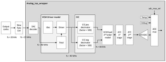
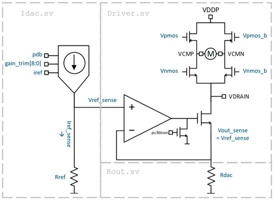
The VCM driver discussed in this paper is located in the broader context of a complete analog signal processing path, as illustrated in Figure 1.

Figure 1. System-level context—analog top wrapper.

Figure 1 shows the key components of the analog signal path, along with the sampling frequency (fs) information across the chain.

• Analog_top_wrapper—Top-level container for all FPGA-based analog behavioral models.
• DAC decoder—(fs = 20 MHz)—Digital interface block translating the control codes into DAC-style signals.
• VCM driver model (fs = 40 MHz)—Behavioral fixed-point model of the VCM output driver.
• Idac—Iref_sense and Vref_sense generation model for the VCM driver.
• Rout—Output RDAC resistance model.
• Driver—Combines the current source and output resistance effects with digital control. It generates differential driver output signals that feed the downstream load and decimation stages.
• CIC block (fs = 40 MHz → 80 kHz)—Cascaded Integrator-Comb (CIC) decimation filters.
• VCM load 2nd order model (fs = 80 kHz)—Fixed-point behavioral model of the VCM electrical load. It is configured with parameterized fixed-point biquad coefficients.
• AFE 1st and 2nd stage—First and second analog front-end stage conditioning the output of the load model with the programmable gain from the digital core.
• SAR ADC (fs = 80 kHz)—Behavioral model of the ADC sampling the VCM load response. It converts the analog equivalent fixed-point load signal into digital output samples for system-level verification. The output of the SAR ADC is mux-ed with temperature and debug information through an auxiliary multiplexer.

Outside the analog_top_wrapper, the blocks “Output codes” and “Slew rate ctrl” are located in the digital top section of the SoC and control the analog signal path through digital binary codes to obtain the desired positioning of the VCM load.

The workflow that leads to the implementation of the digital model includes steps such as collaboration with analog designers to extract the mathematical descriptions of the analog design and the electrical dynamics; conversion of real-number models into fixed-point representations, choosing the word lengths and the scaling based on accuracy requirements; implementation in SystemVerilog with the synthesis constraints in mind (latency, pipelining, area); deployment and verification on FPGA, comparing the results against the analog reference simulations.

The manual RTL fixed-point model discussed in the paper is a redesign of a previous implementation approach designed with an automated high-level RTL generation flow, which makes use of the SVREAL library (referred to as “real-number modeling” in the following sections). The aim of the new manual RTL fixed-point implementation is to reduce the area and timing results obtained with the automated approach by letting the designer explore optimization opportunities such as pipelining and tailored resource utilization. From a system perspective, the new redesign needed to have more efficient area utilization with the goal of replicating the entire analog signal path into multiple independent instances on a new and bigger system, while using the same FPGA platform. Moreover, it was desired to have precise control of the Clock-Domain Crossing (CDC) [34,35] points of the design, since multiple clock sources are used in the final system and the explicit handling of the critical crossing points in RTL was not included in the autogenerated real-number approach. The CDC points are indeed critical for a working design and are subtle sources of failure that can lead to long debug times.

From a project-level perspective, the motivation for this work is to prepare a functioning analog hardware model so that it is ready to be used for firmware development and digital hardware design of the final mixed-signal chip. This approach can reduce risk and anticipate expected behavior after silicon manufacturing.

In general, creating an RTL model manually is advantageous in mixed-signal design practice. In fact, it enables the real-time emulation of analog circuits, which is unfeasible with traditional analog simulation tools; it allows early firmware development, closed-loop controller testing and fault analysis before silicon; and it supports co-simulation for system designers.

In summary, this work presents a quantitative comparison of a manually encoded fixed-point digital model of a VCM driver against an implementation with an automatic approach in real-number modeling, evaluating the trade-offs. The results of the FPGA implementation are finally shown and compared to those of a previous automated real-number implementation. A comparison of the fixed-point model output against the behavioral analog equation is also provided, to quantify the model fidelity.

The remainder of this paper is organized as follows. Section 2 presents the circuit and the methodology used for translating the analog behavioral descriptions into synthesizable fixed-point RTL implementations, including the fixed-point representation strategy and the optimization techniques adopted to improve the FPGA implementation efficiency. The application of the methodology is shown through representative blocks of the VCM driver model. Section 3 presents the FPGA implementation results and compares the manually optimized fixed-point RTL implementation with a previously developed MSDSL/SVREAL-based implementation in terms of resource utilization and quantifies the error of the fixed-point model against the analog behavioral model. Section 4 discusses the observed trade-offs and implications for the FPGA-based analog emulation. Finally, Section 5 concludes the paper.

2. Materials and Methods

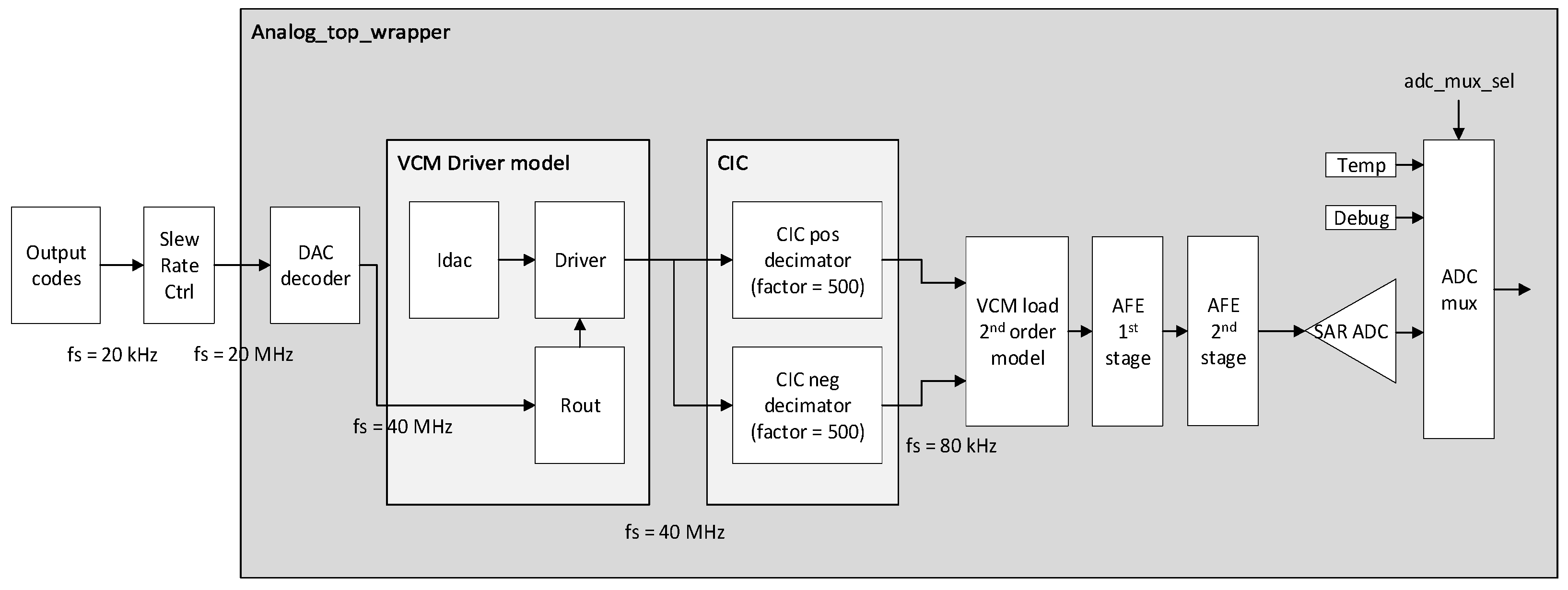
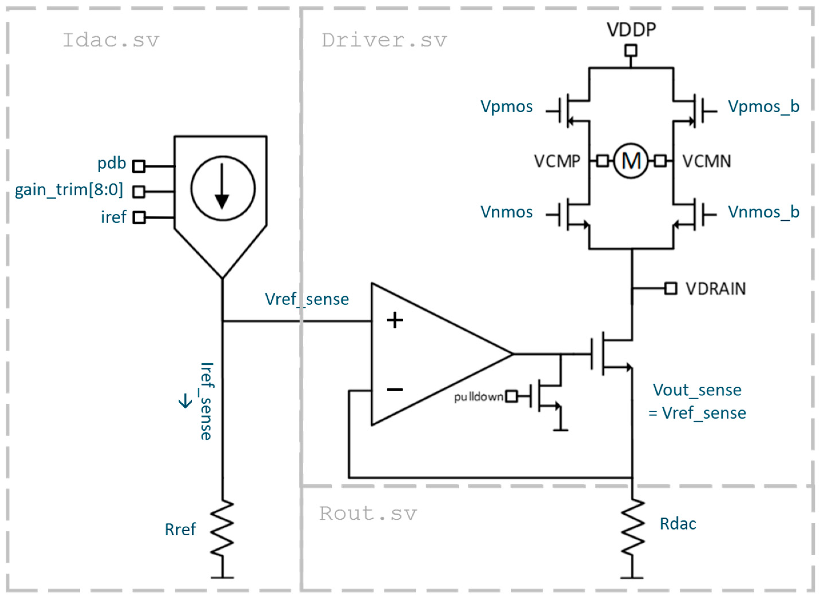
The digital fixed-point model presented in this paper is based on the analog circuit shown in Figure 2, in reference to the system-level analog_top_wrapper module depicted in Figure 1. Encircled in dashed lines are the names of the SystemVerilog digital blocks which implement the underlying analog sub-circuit, which will be explained in the following paragraphs.

Figure 2. VCM driver analog circuit and subdivision in SystemVerilog modules.

The analog circuit in Figure 2 implements a differential Voice Coil Motor (VCM) driver. The circuit is a bi-directional current driver supplied by the VDDP pin.

Inside the block Driver.sv, the circuit is composed of the following:

• A driver loop OTA, which regulates the driver output current;
• An output stage, consisting of ahigh-voltage NMOS and a PMOS for polarity change and an NMOS for output current regulation;
• The actual load M, modeled as a series of inductance and resistance.

The output current is modulated by a monotonic DAC.

Inside the block Rout.sv is an RDAC decoder, which sets the output resistance to generate the output current given an input driver code. The 10-bit driver code is converted to 5-bit binary cell control and 31-bit segmented cell control.

Inside the driver RDAC, a current DAC is used to trim the current reference used to generate the reference voltage of the main driver loop.

Inside the block Idac.sv, the signal gain_trim [8:0] is a trimming control signal used to trim the driver load current to a trimming target.

To aid the transition from analog circuits to digital models, the analog team provided equations which fully characterize the essential behavior of the analog circuit. The equations were used as a source of truth and were approximated with fixed-point representation in RTL to reproduce the analog behavior in digital form.

The aim of the following subsections is to provide the architectural strategies used in the implementation of a subset of blocks to illustrate how the key concepts of manual fixed-point modeling were translated into actual hardware. The Idac and Rout blocks are simple yet detailed enough for this goal and contain sufficient design opportunities to illustrate the general fixed-point design decisions taken.

References [36,37] and Appendix A offer an introduction to the fixed-point concepts and terminology used throughout the following sections.

2.1. Hardware-Efficient Optimization Flow

The manual implementation of the VCM driver leveraged established fixed-point RTL design practices, summarized by the following optimization principles:

• Compile-Time Evaluation

The analog equations to be modeled are evaluated and static parts are extracted; so that they can be evaluated during elaboration and encoded as constants, eliminating unnecessary arithmetic logic. Compile-time functions can be used to refine the constant values to the desired precision.

• Algebraic Reformulation

The analog equations are manipulated to reduce computational complexity and minimize arithmetic depth. The reformulation is also aimed at revealing as many static compile-time encoding opportunities as possible.

• Arithmetic Simplification

Multiplication and division operations are replaced by shifts and additions whenever possible.

• Divider Minimization

Divisions are isolated, precomputed, or reformulated to reduce logic utilization and critical-path delay. Wrapper modules can be used to select a simulation-oriented or an FPGA-optimized divider block, depending on the scenario.

• Bit-Width Optimization

Each signal is assigned the minimum width satisfying dynamic-range and precision requirements across the entire computational chain.

• Pipeline-Aware Mapping

Arithmetic stages are partitioned to improve timing closure and maximize FPGA operating frequency.

In the following subsections, representative blocks Idac and Rout are used as a case study to illustrate the application of the above optimizations.

2.2. Hardware-Efficient Optimization Case Study: Idac Block

The Idac block encapsulates sufficient complexity to benefit from optimization principles such as compile-time evaluation, algebraic reformulation, arithmetic simplification, divider minimization and bit-width optimization. These principles can directly be applied by observing the analog modeling equation.

2.2.1. Reference Equations for the Idac Block

The Idac block provides the current i_ref,sense, from which the v_ref,sense voltage can be calculated, as shown in Figure 2. To calculate the current i_ref,sense, the current nodes of the DAC are modeled as follows:

$$\begin{gathered} D_0=\mathrm{gain}\text{\_}\mathrm{trim}\left[0\right]?{\displaystyle \frac{1}{8}}:0 \\ {D}_1=\mathrm{gain}\text{\_}\mathrm{trim}[1]?{\displaystyle \frac{1}{4}}:0 \\ \dots \\ {D}_8=\mathrm{gain}\text{\_}\mathrm{trim}\left[8\right]?32:0 \end{gathered}$$

(1)

Considering the value of i_ref = 8 µA and including the signal pdb (inverted power-down), the following equations are given to calculate i_ref,sense:

$$\begin{gathered} i_{\mathrm{ref},\mathrm{sense},\mathrm{aux}}=i_{\mathrm{ref}}·\left(66+D_0+D_1+\dots +D_8\right) \\ {i}_{\mathrm{ref},\mathrm{sense}}=\mathrm{pdb}?i_{\mathrm{ref},\mathrm{sense},\mathrm{aux}} :0 \end{gathered}$$

(2)

The final v_ref,sense is then calculated by multiplying

$$v_{\mathrm{ref},\mathrm{sense}}=i_{\mathrm{ref},\mathrm{sense}}·R_{\mathrm{ref}}$$

(3)

where R_ref = 56 Ω in our implementation.

2.2.2. SystemVerilog Implementation and Optimization Flow of the Idac Block

The first step in implementing the equations is range analysis across the VCM driver processing chain. The chosen fixed-point format for the blocks under analysis is Q10.22, with sign included. The reason for this format stems from the analysis of the required dynamic range of the quantities appearing in the modeling equations. The integer width (9 bits excluding sign) is determined by the maximum resistance value in the data-path, corresponding to R_out at minimum DAC code, where only the smallest binary conductance weight ${\displaystyle \frac{1}{8·R_{\mathrm{unit}}}}$ is active, yielding R_out,max = 8 × R_unit = 8 × 28.071 ≈ 224.6 Ω (see Section 2.3 for the Rout block). This requires ⌈log₂(225)⌉ = 8 bits excluding sign, rounded to 9 for headroom. Since a convenient 32-bit total word was selected as the implementation target for consistency across the design, the remaining 22 bits were allocated to the fractional part, therefore yielding the Q10.22 format (1 sign + 9 integer + 22 fractional).

The fractional word length of 22 bits yields a quantization step of 2⁻²² of the represented quantity. Applied to the current quantities modeled in this block, it corresponds to an LSB of approximately 0.238 µA. Considering the external analog requirement to retain precision down to 0.1 ILSB (where ILSB ≈ 195.5 µA with 1023 possible DAC codes), and an internal design target of 1 µA precision, the resulting LSB weight was therefore considered sufficient, as it is approximately 82× smaller than the external specification limit of 19.55 µA and approximately 4.2× smaller than the internal design target of 1 µA. The adequacy of the selected format was subsequently verified through the accuracy analysis presented in Section 3.2, which showed a peak modeling error substantially below the 0.1 ILSB requirement.

Compile-time evaluation and algebraic reformulation: The modeling Equations (1)–(3) could be algebraically manipulated to isolate constant quantities that do not depend on gain_trim [8:0], which is variable. That is, the quantities i_ref × R_ref × 66 and i_ref × R_ref can be separately pre-computed at elaboration time with the desired precision, for instance, using 64-bit integer arithmetic within SystemVerilog constant functions. The results are encoded directly as fixed-point constants (localparams), eliminating two of the three multiplications from the run-time data-path entirely. A code example would be

localparam logic signed [TOTAL_BITS-1:0] Iref_66_Rref_fxp = compute_iref_66_rref();

localparam logic signed [TOTAL_BITS-1:0] Iref_Rref_fxp = compute_iref_rref_hp(); //high-precision

The parameter R_ref is specified in mΩ units (parameter RREF_MOHM = 56,000) to provide sub-Ohm calibration resolution without requiring real-number type evaluation or non-synthesizable constructs such as $rtoi.

Arithmetic simplification: Considering the definition of gain_trim as in Equation (1), the numerical value of gain_trim in the v_ref,sense equation is obtained with a division by 8. The division in the gain_trim term can be implemented as an arithmetic right-shift by 3 bits (>>>3), avoiding a hardware divider. Since the scaling coefficient i_ref × R_ref is pre-computed as fixed-point, multiplication by (gain_trim >>> 3) would still be a fixed-point number multiplied by a scaling factor; therefore, there is no required scaling back to the right by FRAC_BITS. As a result, no run-time division hardware is inferred.

Divider minimization: Since only v_ref,sense is needed for the Rdac block, i_ref,sense can be calculated as an observation-only back-computation. The equation i_ref,sense = v_ref,sense/R_ref is reformulated as a multiplication by the pre-computed reciprocal 1/R_ref, encoded at elaboration time as a fixed-point constant. This eliminates the sole division in the block, replacing it with a single multiplier:

localparam logic signed [TOTAL_BITS-1:0] Rref_rec_fxp = compute_rref_rec_fxp();

assign Iref_sense_tmp = Vref_sense_pdb * Rref_rec_fxp;

Pipeline-aware mapping: The Idac block data-path is purely combinational with a single output register stage, as the computation reduces to one multiplier (gain_trim × constant) and two additions after compile-time evaluation. This single-cycle latency is consistent with the downstream Rout and Driver stages, enabling uniform pipeline alignment across the full driver chain.

To summarize, through the above optimizations, the Idac block reduces from a three-multiplier, one-divider floating-point expression to a single run-time multiplier and two adders, with all remaining parameters resolved as elaboration-time constants.

2.3. Hardware-Efficient Optimization Case Study: Rout Block

The implementation of the Rout block will be discussed in this subsection to illustrate the application of the optimization flow as done for the Idac block.

2.3.1. Reference Equations for the Rout Block

The Rout block implements the R_DAC variable output resistance of the Driver block, driven by the DAC Decoder block with a 5-bit binary code and a 31-bit thermometer code, as shown in Figure 1 and Figure 2. The binary and thermometer codes are input into the Rout block as signals:

data_out_b [30:0]

code_buf_b [4:0].

The _b notation indicates that both signals are to be considered in inverted form. The simplified modeling equations to calculate the R_out value from the binary and thermometer codes are shown below:

$$\begin{gathered} R_{\mathrm{unit}}=28.07112 \mathsf{\Omega } \\ (C_0=8·R_{\mathrm{unit}}, C_1=4·R_{\mathrm{unit}}, \dots , C_4={\displaystyle \frac{1}{2}}·R_{\mathrm{unit}})\&!\mathrm{code}\text{\_}\mathrm{buf}\text{\_}\mathrm{b}[n] \\ {D}_n (\mathrm{f}\mathrm{o}\mathrm{r} \mathrm{a}\mathrm{l}\mathrm{l} n)={\displaystyle \frac{1}{4}}·R_{\mathrm{unit}}\&!\mathrm{data}\text{\_}\mathrm{out}\text{\_}\mathrm{b}[n] \end{gathered}$$

(4)

As an example, if data_out_b [0] == 0, D₀ = ${\displaystyle \frac{1}{4}}·R_{\mathrm{unit}}$; if not, that impedance is not connected. Similarly, this applies for C₀, …, C_n.

The final R_dac output value is obtained by calculating the parallel of the equivalent C_eq and D_eq (code and data) calculated from the equations above.

$$R_{\mathrm{dac}}=C_0//\dots //{\mathrm{C}}_4//D_0//D_1//\dots //D_{30}$$

(5)

A direct implementation of the modeling equations would suggest that 36 + 1 run-time division operators are needed to implement them in hardware (one per segment to compute each conductance, plus the final reciprocal).

2.3.2. SystemVerilog Implementation and Optimization Flow of the Rout Block

Algebraic reformulation: The original expression involves 36 individual resistance-to-conductance conversions followed by a summation. By reformulating in the conductance domain, the computation becomes a pure summation of pre-computed constants gated by the decoder bits, since R_unit is a physical constant of the circuit. We express the parallel resistance calculation in Equation (5) as

$${\displaystyle \frac{1}{R_{\mathrm{eq}}}}=G_{\mathrm{eq}}={\displaystyle \frac{1}{R_1}}+{\displaystyle \frac{1}{R_2}}+\cdots +{\displaystyle \frac{1}{R_n}}$$

(6)

Since each gating factor is a single bit as shown in Equation (4), the multiplications reduce to conditional additions (mux-to-zero), requiring no multiplier hardware.

$$G_{\mathrm{eq}}={\displaystyle \sum _{i=0}^4}\overline{\mathrm{code}\text{\_}\mathrm{buf}\text{\_}\mathrm{b}\left[i\right]}\cdot C_{\mathrm{inv},\mathrm{f}\mathrm{x}\mathrm{p}}\left[i\right]+{\displaystyle \sum _{k=0}^{30}}\overline{\mathrm{data}\text{\_}\mathrm{out}\text{\_}\mathrm{b}\left[k\right]}\cdot D_{\mathrm{inv},\mathrm{f}\mathrm{x}\mathrm{p}}.$$

(7)

The final R_dac value can be obtained by adding the gated inverted C[n] and D[m] addends together and by inverting the result of the addition.

Compile-time evaluation: Since the C_eq and D_eq equivalents are calculated by means of a static R_unit value, all per-segment conductance weights can be fully resolved at elaboration time and pre-calculated with the desired precision. For instance, a single parameterized constant function (compute_cfxp) can be used to evaluate

$$\mathrm{round}\left(M\cdot 2^{\mathrm{FRAC}\text{\_}\mathrm{BITS}}/R_{\mathrm{unit},\mathrm{m}\mathsf{\Omega }}\right)$$

(8)

This is completed using 64-bit integer arithmetic, where M encodes the segment scaling factor in milli-Siemens × 1000 units and R_unit is a parameter encoded in mΩ precision. This produces six fixed-point constants:

$$C_{0,\mathrm{inv},\mathrm{fxp}}={\displaystyle \frac{1}{\left(8\cdot R_{\mathrm{unit}}\right)}},\dots ,C_{4,\mathrm{inv},\mathrm{fxp}}={\displaystyle \frac{2}{R_{\mathrm{unit}}}};D_{\mathrm{inv},\mathrm{fxp}}={\displaystyle \frac{4}{R_{\mathrm{unit}}}}$$

(9)

All 36 per-segment conductance computations reduce to constant lookups, eliminating every division from the conductance summation path.

Divider minimization and optimization: The sole remaining division in the block is the final reciprocal $R_{\mathrm{out}}=1/G_{\mathrm{eq}}$, which converts the accumulated conductance back to resistance for the downstream Driver stage. This division cannot be algebraically eliminated because $G_{\mathrm{eq}}$ is code-dependent and varies across the full DAC range. The division operator can be encapsulated into a wrapper block with different implementations, depending on the scenario (for instance, an optimized Xilinx FPGA divider instance and an inferred sequential model for simulation only, differentiated by an `ifdef condition). The divider represents the only non-trivial arithmetic resource in the block.

Pipeline-aware mapping: The conductance accumulation (36 conditional additions) is purely combinational and completes within a single clock cycle. The sequential divider operates over multiple cycles and signals completion via a done flag, after which the output register captures the result. This partitioning isolates the long-latency division from the combinational summation, enabling the upstream decoder and downstream Driver to operate at full clock rate without back-pressure.

Through conductance-domain reformulation and compile-time constant pre-computation, the R_out block reduces from 36 run-time divisions to zero, replacing them with 36 single-bit conditional additions and one sequential divider for the final reciprocal. The run-time data-path contains no multipliers, and the only division is the irreducible $1/G_{\mathrm{eq}}$ conversion at the output. A divider wrapper block can be useful to hide the details of the division circuit employed and can offer different implementations such as FPGA-optimized, pipelined, inferred or simply different algorithms.

2.4. Translating a Floating-Point SAR ADC Model to Fixed-Point: Step by Step

This Section documents the decisions made when translating the auto-generated floating-point SAR ADC model (produced by MSDSL/SVREAL) into a manually written fixed-point equivalent.

The transfer function being implemented is

$$d_{\mathrm{out}}= \mathrm{clamp}\left({\displaystyle \frac{(V_{\mathrm{in},\mathrm{p}}-V_{\mathrm{in},\mathrm{n}}+V_{\mathrm{ref}})}{(2 · V_{\mathrm{ref}})}} · 65535, 0, 65535 \right)$$

(10)

2.4.1. Choosing the Fixed-Point Format

The first decision, which does not exist in the floating-point version, is selecting the number representation.

• What floating-point does:
  The SVREAL macros declare ports with DECL_REAL/INPUT_REAL, which under VIVADO_FLOAT mode are expanded to 32-bit IEEE-754 single-precision signals. The range is ±3.4 × 10³⁸ with ~7 significant decimal digits. No decision is required from the designer; the format is universal.
• What fixed-point requires:
  The designer must choose a Q-format, the number of integer bits and the number of fractional bits to allocate. For the SAR ADC, Q4.28 was selected. The 28 fractional bits yield a resolution of 2⁻²⁸ ≈ 3.73 nV, far more than the 16-bit ADC output requires. The extra precision was chosen to ensure that rounding errors in intermediate operations do not accumulate enough.

Key difference: In floating-point, the exponent field automatically adjusts the scale of every signal at every stage. In fixed-point, the Q4.28 format is chosen once and applies to all input ports; the designer must verify that no input ever exceeds, or the value wraps silently.

2.4.2. Differential Subtraction: V_in,p − V_in,n

• Floating-point:
  The auto-generated code computes the difference in two steps: negate V_{in_n}, then add to V_{in_p}. Negation is a single-bit operation (flip bit 31); addition is a Vivado IP core. No width management is needed.
• Fixed-point:
  Subtraction of two 32-bit signed values can overflow by 1 bit. The result must be 33 bits to avoid truncation.

Key difference: Floating-point subtraction cannot overflow for values in this range (the exponent adjusts). Fixed-point subtraction requires the designer to add a guard bit and widen the result.

2.4.3. Offset Addition: V_diff + V_ref

• Floating-point:
  Use the ADD_REAL, same IP core, same 32-bit container.
• Fixed-point:
  Adding a 33-bit result to a 32-bit input can again overflow. The result grows to 34 bits.

Key difference: After just two operations (one subtraction, one addition), the fixed-point signal has grown from 32 to 34 bits. In floating-point, the signal is still 32 bits. This width tracking must continue through every subsequent operation, and it compounds.

2.4.4. Computing the Denominator: 2 × V_ref

• Floating-point:
  Multiplying by 2 is a MUL_CONST_REAL; it instantiates a Vivado floating-point multiplier IP core.
• Fixed-point:
  Multiplying by 2 in fixed-point is simply a left shift by 1. No IP core, no multiplier, and no extra resources are needed.

Key difference: This is one case where fixed-point is simpler than floating-point. A constant power-of-two multiply is free in fixed-point; it is just a wire shift. In floating-point, it still instantiates a full multiplier IP core.

2.4.5. Division: V_samp/(2 × V_ref)

This is where the translation becomes fundamentally different.

• Floating-point:
  Division is a single macro that instantiates a Vivado floating-point divider IP. The IP core handles arbitrary operand magnitudes, produces a correctly rounded result, and returns ±∞ on division by zero. It is pipelined internally and signals completion via valid/ready handshake.
• Fixed-point:
  Integer division truncates the fractional part of the result. To preserve precision, the numerator must be pre-scaled by shifting it left by FRAC_BITS positions before dividing. This ensures that the quotient retains 28 fractional bits but creates a wide intermediate value. Without this pre-scaling, dividing two Q4.28 numbers would produce a result with zero fractional bits, essentially a truncated integer.

Key difference: In floating-point, division is a single macro call with one line, no scaling, no width management, and well-defined behavior on edge cases. In fixed-point, it is the most complex part of the design: the designer must pre-scale the numerator, manage the data-path, and handle the quotient extraction.

2.4.6. Scaling by 65,535: Ratio × 65,535

• Floating-point:
  Use the MUL_CONST_REAL, which is the same as any other constant multiplication.
• Fixed-point:
  A general multiplier would require a wide multiplication (32 × 17 bits). Instead, the fixed-point version exploits the algebraic identity:

  $$\begin{gathered} 65535=2^{16}-1 \\ n·65535=(n\ll 16)-n \end{gathered}$$

  (11)

This replaces a multiplier with a shift (free, just wiring) and a subtractor.

Key difference: This is where manual fixed-point design shines. The designer can exploit structure in the constants to eliminate hardware. Floating-point treats 65,535.0 the same as any other constant, it always instantiates a full multiplier IP core.

2.4.7. Clamping to [0, 65,535]

• Floating-point:
  Clamping is expressed as max(value, 0) then min(result, 65,535), using the MAX_REAL and MIN_REAL macros. These instantiate floating-point comparator IPs and muxes, operating on real-valued signals. There is no ambiguity: the comparison is on real-valued numbers, and the result is the larger/smaller of the two.
• Fixed-point:
  Clamping requires comparing the fixed-point value against bounds, then extracting the integer part via right-shifting.

Key difference: In floating-point, clamping is a simple min/max on real values. In fixed-point, the designer must: (a) compute the clamp bounds in the correct fixed-point scale, (b) handle the signedness of the comparison correctly, and (c) extract the integer portion via shifting with the right number of fractional bits.

3. Results

3.1. FPGA Area Comparison: Manual Fixed-Point RTL vs. Automatic SVREAL Generated RTL

The full mixed-signal digital path shown in Figure 1 was synthesized and implemented on a Xilinx ZCU104 Evaluation Kit FPGA platform [38], which features a Zynq UltraScale+ XCZU7EV device with the resources listed in Table 1.

Table 1. Xilinx Zynq FPGA platform used.

Resource	Type/Amount
CPU	Quad ARM A53 Cortex dual ARM R5 Cortex
System Logic Cells (K)	504
Memory	38 Mb
DSP Slices	1728
Maximum I/O Pins	464

To quantify the implementation cost of the manual fixed-point RTL modeling flow, Table 2 shows the FPGA LUT resource utilization results of the manual fixed-point compared against the prior implementation of the same functionality generated using an automated RTL generation flow leveraging the SVREAL library (hereafter, “real-number flow”).

Table 2. FPGA resource utilization comparison: total LUTs.

Name	Fixed-Point Total LUTs	Real Total LUTs	% Diff FxP vs. Real Total LUTs
analog_top_wrapper	3003	18,649	−83.90%
dac_decoder	5	0	/ 1
adc_top	963	1492	−35.46%
cicp	70	279	−74.91%
cicn	34	277	−87.73%
VCMLoad2Order	429	1602	−73.22%
Rout	389	6715	−94.21%
IDac	19	330	−94.24%
Driver	675	6854	−90.15%
AFE_SecondStage	134	171	−21.64%
AFE_FirstStage	95	125	−24.00%

¹ dac_decoder contribution negligible for total LUTs.

The comparison covers the analog_top_wrapper modeling island, which contains the DAC decoder, the Driver, the CIC decimators, the second-order VCM load model, the analog front-end (AFE) blocks, and the SAR ADC model.

The manual fixed-point redesign from the real-number flow brought the following changes in resource utilization:

• Total LUTs reduce from 18,649 (real-number flow) to 3003 (fixed-point), corresponding to −83.9%;
• FFs reduce from 6631 to 2641 (−60.2%);
• CLBs reduce from 3364 to 722 (−78.5%);
• DSP usage reduces from 166 to 87 (−47.6%).

These reductions are consistent with the design choices described in the Methods section: (i) static-quantity pre-encoding as compile-time constants, (ii) algebraic equation rearrangements to replace general arithmetic with shifts/adds, and (iii) minimizing divider instantiations by using reciprocals and a single division point only where strictly required.

A per-block look highlights that the largest contributors to the real-number overhead are exactly the blocks that contain repeated multiplications/divisions and wide dynamic range operations.

RDAC/Rout is the most striking example:

• Total LUTs: 6715 → 389 (−94.2%);
• FFs: 2735 → 208 (−92.4%);
• DSPs: 80 → 12 (−85.0%).

This aligns with the modeling strategy in which the parallel resistance is reformulated to sum reciprocals and perform only one final inversion while exploiting a precomputed reciprocal of R_unit.

Similarly, the Driver block shows a near order-of-magnitude reduction.

The Idac block also exhibits a dramatic reduction. This is consistent with identifying and implementing the constant quantities as compile-time fixed-point parameters and avoiding costly divisions.

For the signal-processing blocks (CIC decimators and second-order VCM load model), the reductions remain substantial.

These results indicate that the fixed-point arithmetic and the explicit width/range design reduce the need for the generic operators that the real-number flow maps to heavy combinational logic or additional DSP-assisted data-paths.

3.2. Accuracy Verification

The fixed-point VCM driver model was validated against the ideal behavioral transfer function

$$I_{\mathrm{out},\mathrm{ideal}}\left(\mathrm{mA}\right)=\mathrm{dac}\text{\_}\mathrm{code}\cdot {\displaystyle \frac{200\mathrm{mA}}{1023}}$$

(12)

This was completed over the full 10-bit code space with the parameters R_ref = 56 Ω, R_unit = 28.071 Ω. The validation was performed with gain_trim [8] asserted (therefore, gain_trim = 9′b100000000). According to Equation (1), this activates the DAC weighting contribution D₈ = ‘d32 units. A simulation sweep covering 513 uniformly spaced codes (0 to 1023, step 2) from a real use-case was performed, with the steady-state output current of the fixed-point chain (Idac → Rout → Driver) compared against the analytical reference at each operating point. Table 3 shows an extract of the code sweep and Table 4 summarizes the error metrics.

Table 3. Fixed-point VCM driver model accuracy—full code sweep.

DAC Code	Iout,fxp (mA)	Iout,ideal (mA)	Abs. Error (µA)	Error (ILSB)
0	0.000000	0.000000	+0.000	+0.00000
1	0.195265	0.195503	−0.239	−0.00122
3	0.586271	0.586510	−0.239	−0.00122
5	0.977516	0.977517	−0.001	−0.00000
9	1.759529	1.759531	−0.002	−0.00001
15	2.932549	2.932551	−0.003	−0.00001
31	6.060600	6.060606	−0.006	−0.00003
63	12.316704	12.316716	−0.012	−0.00006
127	24.828911	24.828935	−0.024	−0.00012
255	49.853563	49.853373	+0.190	+0.00097
511	99.902868	99.902250	+0.618	+0.00316
767	149.951935	149.951130	+0.805	+0.00412
1019	199.219227	199.217990	+1.237	+0.00633
1021	199.610233	199.608997	+1.237	+0.00633
1023	200.001240	200.000003	+1.237	+0.00633

Table 4. Summary error metrics.

Metric	Value	ILSB Fraction
Full-scale range	200 mA	1023 LSBs
LSB step size (ILSB)	195.50 µA	1.000
Peak absolute error	1.252 µA (code 925–963)	0.0064
RMS error	0.662 µA	0.0034
Mean absolute error	0.540 µA	0.0028
External accuracy requirement	19.55 µA	0.1000
Margin to spec	15.6×	-

The peak error of 1.252 µA occurs exclusively in the upper code range (codes 925–963), where the accumulated conductance in the Rout stage is largest and the fixed-point reciprocal division contributes its maximum quantization residual. The error distribution is highly uniform: all ten of the worst-case codes exhibit an identical 1.252 µA deviation, indicating a systematic quantization floor rather than isolated numerical anomalies.

The dominant error source is the mΩ rounding of the unit resistance parameter ($R_{\mathrm{unit},\mathrm{m}\mathsf{\Omega }}=28071$, representing 28.071 Ω versus the ideal 28.07112 Ω), which introduces a 4.3 ppm gain error that scales linearly with the output current. At full scale (200 mA), this contributes approximately 0.86 µA—consistent with the observed peak error when combined with the ±0.5 LSB quantization noise of the 22-bit fractional representation.

The 15.6× margin to the 0.1 ILSB external accuracy requirement confirms that the 32-bit Q10.22 fixed-point format, combined with the compile-time constant pre-computation and the mΩ parameterization strategy, provides adequate numerical fidelity for the intended application without requiring floating-point arithmetic or extended word widths.

4. Discussion

4.1. Trade-Offs and Secondary Effects

While the overall trend strongly favors the manual fixed-point RTL, some blocks show resource redistribution rather than uniform reduction.

• The SAR ADC model (adc_top) reduces the LUTs (1492 → 963, −35.5%) but increases the FFs (788 → 1023, +29.8%) and the DSPs (8 → 19, +137.5%).
  A plausible interpretation is that the manual fixed-point implementation introduces additional pipelining and/or uses DSP blocks more aggressively for deterministic arithmetic, shifting the cost from LUTs to registers/DSPs while still improving the overall LUT footprint.
• The AFE stages show moderate LUT reductions (≈−22% to −24%) but the DSP usage doubles (4 → 8) in both first and second stages.
  In practice, this can be an acceptable trade if the platform is LUT-limited and has DSP headroom, and it reflects how explicit fixed-point multipliers often infer DSPs by construction.

The real-number flow provides the rapid prototyping of analog equations into synthesizable RTL with designer effort involved in the high-level programming language modeling, such as Python, rather than the hardware-specific details in direct RTL. This offers significantly shorter development times in mixed-signal modeling and can be especially advantageous during the initial development and exploration stage. However, substantial hardware costs will need to be factored in, as the generic operators required to support the wide dynamic range, the implicit scaling, and divisions are mapped to LUT heavy combinational logic and frequent DSP instantiations. Designers might therefore be prevented from leveraging optimization and simplification opportunities, such as when the underlying equations contain static coefficients or structurally redundant computations, whose data-path can be optimized with pipelining or other strategies.

On the other hand, the manual fixed-point RTL approach exposes the designer to the analysis and choice of range and fractional parts, as well as scaling and operator intent at design time. Despite this requiring greater effort from the outset, such as understanding the equations to model and the word-length selection, the FPGA resource usage can be significantly reduced. The designer is in control of the RTL implementation of the equations in such a way as to make the hardware implementation more closely reflect the physical intent of the analog model with essential hardware. The large reductions observed in LUTs, CLBs, and DSPs—especially in the computation-intensive blocks such as RDAC/Rout, Driver, and Idac—can be used as an example.

4.2. CDC Considerations in Mixed-Signal FPGA Emulation

Another critical difference between the two approaches is, as mentioned in the Introduction, the explicit identification and handling of the Clock-Domain Crossing (CDC) and Reset-Domain Crossing (RDC) points [34,35,39,40]. Since the Analog_top_wrapper is, by system design, agnostic of the clock domains used in the digital core section and in the DAC decoder block, care must be taken in ensuring that all the parts of the analog paths receive synchronized data with appropriate synchronization structures, such as reset and data synchronizers, qualifiers and FIFOs. The automated approach did not include CDC structures in the RTL generation; therefore, it is of utmost importance that the designer factor this in while developing the analog fixed-point models with a manual approach. Indeed, CDC points, when not properly handled, are the likely cause of the design not working as expected when implemented and deployed onto real silicon, leading to potentially long debug sessions.

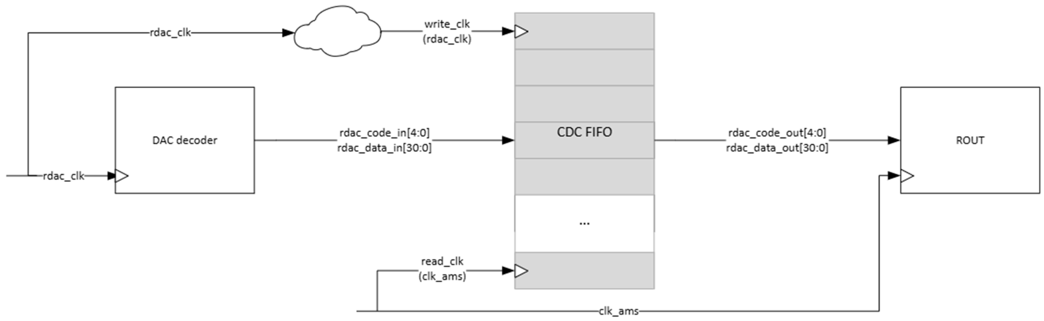
Figure 3 provides a diagram of the CDC handling strategy used between the DAC decoder block and the Rout block in the manual design. The DAC decoder operates in the rdac_clk domain, whereas the analog modeling chain operates in the clk_ams domain, with both domains being unrelated. Consequently, decoder outputs must cross a Clock-Domain boundary before being consumed by the Rout block. In the manually developed RTL implementation, this crossing is explicitly managed through an asynchronous FIFO structure, providing deterministic and elastic synchronization of the multi-bit data and avoiding metastability-related issues.

Figure 3. CDC FIFO between the rdac_clk domain and the clk_ams domain.

4.3. Final Remarks

Overall, the utilization data shows that manual fixed-point RTL modeling can be more area-efficient than a real-number modeling flow for the FPGA implementation of mixed-signal behavioral blocks. Significant savings are concentrated in the blocks that, in their original equation form, rely on repeated division/multiplication and wide dynamic-range computations (notably RDAC/Rout, Driver, and IDac), where optimizations can be leveraged by the designer.

The results support the implementation flow presented in this work—namely, selecting the fixed-point ranges by construction, encoding the static terms at compile time, and restructuring the equations to avoid costly operators—and designers can reap the benefits of a tailored manual RTL approach directly as tangible reductions in LUT, CLB, and DSP usage at both the block and SoC levels, should they opt for a manual RTL encoding approach and provided that the modeling equations lend themselves to optimization and that CDC is properly taken care of.

5. Conclusions

In this work, a validated case study of the FPGA emulation of an analog VCM driver using a manually developed fixed-point RTL implementation has been presented. Representative blocks of the signal chain were used to illustrate how established fixed-point design practices can be applied to translate real-number behavioral descriptions into synthesizable hardware while preserving the accuracy required for mixed-signal verification.

In the second part of the paper, the FPGA resource utilization has been quantified, along with a comparison of the proposed manual RTL approach with a previous implementation of the same functionality, an automated high-level RTL generation flow with the SVREAL real-number library. The model fidelity has also been evaluated by comparing the simulated i_out against the behavioral analog model, showing sufficient precision. The results show an area reduction in favor of the fixed-point approach, and the trade-offs can be identified between abstraction and implementation efficiency, including explicit visibility and control of the CDC and RDC boundaries. Despite the manual approach requiring greater design effort, designers can reap the benefits of the increased architectural control in the form of more efficient and controlled resource utilization.

Appendix A.1. Fixed-Point Basics

Fixed-point arithmetic was chosen to approximate the VCM driver model behavior [36,37]. This section briefly reviews the fundamentals of fixed-point numeric representation as used in FPGA-based digital modeling. The intent is to introduce the terminology and the concepts necessary to understand the modeling choices described in this paper’s sections, rather than to provide an exhaustive treatment.

In the context of FPGA-based emulation, fixed-point arithmetic offers several advantages, such as naturally mapping to FPGA hardware (DSP slices and LUTs), deterministic latency and execution time and lower area and power compared to floating-point while providing more precision than integers only.

As done with decimal numbers, fixed-point arithmetic brings the idea of using a “binary point” to split a binary number into an integer and a fractional part, such as 101.10110, with the point being fixed in position for consistency with all the mathematical operations used in the system. From the hardware point of view, this example number is still an 8-bit integer; what changes is our interpretation of it when converting from and to the real numbers domain. Binary weights are maintained across the digits for both the integer and the fractional part; therefore, in the above example, the digits in the fractional parts will amount to

$$1·{\displaystyle \frac{1}{2}}+0·{\displaystyle \frac{1}{4}}+1·{\displaystyle \frac{1}{8}}+1·{\displaystyle \frac{1}{16}}+0·{\displaystyle \frac{1}{32}}$$

(A1)

This is in real number form, and it will be added to the weights of the integer part, calculated in the same manner.

Throughout this paper, the notation Qx.y will be used consistently, with x being the bit length of the integer part and y being the bit length of the fractional part. As a rule, we will include the sign bit in the integer length. Therefore, with the example notation Q4.28, it is assumed that one bit is used for the sign, the integer part length is 3 bits, and the fractional part length is 28 bits.

As mentioned before, one of the advantages of the fixed-point notation is that binary arithmetic operations can still be used with integer binary numbers, offering a simple and direct mapping to available FPGA resources, such as addition, subtraction and multiplication. While division will need special consideration since direct RTL to FPGA mapping is not trivial, workarounds can be found to obtain divided results and save resources and clock cycles at the same time.

To enter the fixed-point domain from the real domain, the real number we want to convert is scaled up by the fractional amount chosen. For instance, let us consider the real number 512.0. If we were to choose a total length of 32 bits for our binary numbers, split into 1 bit for the sign, 11 bits for the integer part and 20 bits for the fractional part, the fixed-point encoded equivalent would be obtained by multiplying 512.0 by $2^{20}$ and representing the resulting number as a 32-bit integer. To return to the real domain from the fixed-point domain, the reverse operation needs to be done, that is, divide the fixed-point number by $2^{20}$. Note that in SystemVerilog, this is equivalent to performing an arithmetic shift to the left (when multiplying) or to the right (when dividing). In this case, scaling up a real number by the fractional amount is equivalent to writing

32′d512 <<< FRAC_BITS.

Appendix A.2. Math Operations

Appendix A.2.1. Addition

When performing addition and subtraction, both operands must be scaled to have the same number of bits (n) in the fractional part, with m = integer part and n = fractional part. The reason is that fixed-point numbers represent real values as integers, and the fractional bit width tells the binary point position; therefore, adding/subtracting fixed-point numbers with different fractional bit widths will give alignment problems, mixing the integer and fractional parts incorrectly.

For example, let us consider the following numbers:

Q4,2 → xxxx.xx

Q3,4 → xxxx.xxxx

Adding them directly would be meaningless because the fractional bits are not aligned.

The number of bits for the integer part can be different, but if signed values are used, then it will be necessary to sign extend the number with the smallest number of bits to avoid sign errors. Finally, the result of the addition/subtraction will have the same number of fractional bits n, and, since overflow is possible, it will be better to consider an extra bit for the integer part m.

The following numerical example illustrates this concept. Letus consider the numbers (sign included in the integer part):

Signed Q5,3 → A = 5.25 → 0 0101.010

Signed Q4,2 → B = 3.75 → 0 011.11

B has 2 fractional bits, so it needs to be aligned with A, which has 3 fractional bits. We can do so by shifting one bit to the left and keeping the sign consistent:

B <<< 1 = 0 011.11 <<< 1 = 0 011.110

Note:

• Now B is a Q4,3 fixed-point value;
• The symbol <<< in SystemVerilog preserves the sign.

Since we want to do a signed addition, we want to sign extend B to avoid sign errors; we can use the following SystemVerilog keyword and use a signed Q5,3 fixed-point C to store the result and avoid overflow:

C = $signed(A) + $signed(B) =

0 0101.010 +

0 0011.110 =

--------------

0 1001.000

This addition returns the result in Q5,3 = 0 1001.000 = 72 in decimal form, considering the entire binary number. To convert it to the original real number, we calculate 72/2³ = 9.0 in decimal form.

Appendix A.2.2. Multiplication

Multiplication needs special attention, since the operation works with fixed-point numbers as well, but the result requires the sum of the operand bit widths (i.e., double width when both operands are equal size). For instance, let us consider the same operands as in the addition example:

A = 0 0101.010,

B = 0 011.11.

For easier arithmetic, we align both the fractional and integer widths by choosing the larger format (5 integer bits) to obtain a common format in Q5.3 (8 bits). After the alignment,

A_aligned = 0 0101.010 (Q5.3, unchanged),

B_aligned = 0 0011.110 (Q5.3, previously Q4.2).

B has been converted to Q5.3 by performing fractional alignment (arithmetic shift to the left) and by performing sign extension (repeating the MSB to the left to fill the remaining positions) to obtain the same length as the first operand, as done with the addition example. Both operands are now signed Q5.3, 8 bits each.

If we multiply the aligned operands by interpreting them as integers (scale factor = $2^3$), then we obtain the following:

• $A_{\mathrm{int}}=5.25·2^3=42$
• $B_{\mathrm{int}}=3.75·2^3=30$.

In binary form, we obtain the following:

A_int = 00101010 (42)

B_int = 00011110 (30).

Binary multiplication gives the following:

00101010	(8 bits)	x
00011110	(8 bits)	=
0000010011101100	(16 bits)

The result has grown to an 8 × 8 = 16-bit result, after alignment. The raw product equals 1260, in decimal form, without the fixed-point interpretation.

Since both operands were Q5.3, we obtain the following:

• Integer bits: $5+5=10$
• Fractional bits: $3+3=6$.

The result format will be Q10.6 and the total bits will be 16. The binary result interpreted in fixed-point will be:

0000010011.101100 = 1260/$2^6$ = 19.6875.

As a rule, for signed fixed-point multiplication (two’s complement), let

$$\begin{gathered} X_{\mathrm{s}}\in Q(m_1,n_1) \\ {Y}_{\mathrm{s}}\in Q(m_2,n_2) \end{gathered}$$

(A2)

then

$$Z_{\mathrm{s}}=X_{\mathrm{s}}\times Y_{\mathrm{s}}\in Q(m_1+m_2,\hspace{0.25em}\hspace{0.25em}{n}_1+n_2).$$

(A3)

The multiplication is performed on signed integers, using two’s complement arithmetic as follows:

$$Z_{\mathrm{real}}={\displaystyle \frac{\mathrm{signed}\left(X_{\mathrm{int}}\right)\cdot \mathrm{signed}\left(Y_{\mathrm{int}}\right)}{2^{n_1+n_2}}}$$

(A4)

Sign extension must be applied before multiplication.

After multiplying both operands and obtaining a Q format with double the bits, we need to get back to the original format. To get back to the original format, it is necessary to normalize the result; this can be done by shifting right to get the fractional bit size you need (i.e., n₁ = 30 and n₂ = 30, then the result has 60 bits for the fractional part and it is necessary to shift right by 30 to get back to 30 bits for the fractional part); this aligns the integer part to the target format and reduces the fractional precision.

After the shift, there are two options:

• Truncate (drop extra fractional bits): This is already done by shifting in the previous step so you do nothing more. This is faster but less accurate.
• Round: Check the discarded fractional bits and adjust the last kept bit to make the result closer to the true value. This has better accuracy but slightly more logic.

Finally, in case of an overflow, it is necessary to

• Use a fixed-point value with the integer part big enough to keep the result, or
• Saturate or clip to max/min representable value.

Continuing the example above, we now want to get back to the original format Q5.3, 8 bits. As a reminder, we consider the sign bit included in the integer part. If we used the truncation and saturation approach, we would take the following steps:

Normalize to Q5,3:

• Shift right by 3 → 0 00010011.101 = 157 (in decimal: 157/2³ = 19.625).

Since we do not round, we have just truncated the fractional part.

• This result shows overflow, since the Q5,3 max is +15.875 and we have +19.625. The solution to this is to

→ Use a Q6.3 value to keep the correct result or

→ Saturate to 0 1111.111 = 127 (in decimal form, 127/2³ = 15.875).

• The result after saturation → +15.875.

If we used the rounding and saturation approach, the steps would be as follows:

Normalize to Q5,3:

• Shift right by 3 → 0 00010011.101 = 157 (in decimal: 157/2³ = 19.625).
• Rounding: the MSB of the discarded part (100) is 1. As a rule, if it is 1, we add it to the kept fractional part; otherwise, we do nothing. In our case:
• Discarded part: 100
• MSB: 1

Before rounding: 0 00010011.101 = 157

After rounding: 0 00010011.110 = 158 (in decimal form, 158/2³ = 19.75).

This result shows overflow, since the Q5,3 max is +15.875 and we have +19.75. As in the previous example, the solution to this is to

• Use a Q6,3 value to keep the correct result, or
• Saturate to 0 1111.111 = 127 (in decimal form, 127/2³ = 15.875).

The result after saturation → +15.875.

In the proposed implementation, multiplication is performed using double-width intermediate variables, ensuring that no overflow occurs during the multiplication stage itself. After re-scaling, the result is truncated back to the target fixed-point format. At this stage, overflow may occur if the magnitude of the scaled result exceeds the representable range of the chosen format. If overflow is not explicitly handled through saturation or by using a wider output format, a simple indicator in digital simulations is based on the sign of the result. In two’s complement arithmetic, the product of two operands with the same sign is expected to be positive. Therefore, if both operands are positive or both are negative, and the result after scaling and truncation is negative, then overflow has certainly occurred. It should be noted, however, that this condition is only sufficient and not necessary, as overflow may also occur without a sign inversion when the result magnitude exceeds the representable range but retains the correct sign after truncation.

Appendix A.2.3. Division

In fixed-point arithmetic, division differs from addition and multiplication because it is not scale-preserving, that is, the quotient generally does not inherit the same binary-point position as the operands. While addition and multiplication return predictable bit growth when performed on scaled integers, to maintain precision with division, it is necessary to re-scale the values before performing the operation to preserve fractional resolution. The interpretation of the result is then done in a chosen fixed-point format.

Let the dividend and divisor be represented as

$$\begin{gathered} x=X\cdot 2^{-F_x} \\ y=Y\cdot 2^{-F_y} \end{gathered}$$

(A5)

where $X$ and $Y$ are the stored integers and $F_x$, $F_y$ denote the corresponding numbers of fractional bits. The exact real-valued quotient is

$$q={\displaystyle \frac{x}{y}}={\displaystyle \frac{X}{Y}}\cdot 2^{-(F_x-F_y)}$$

(A6)

Since direct integer division of $X$ by $Y$ would discard the fractional part of the quotient, the dividend must be pre-scaled. If the desired output format has $F_q$ fractional bits, the integer representation of the quotient can be computed as

$$Q=⌊{\displaystyle \frac{X\cdot 2^{F_q+F_y-F_x}}{Y}}⌋$$

(A7)

so that the fixed-point result is interpreted as

$$q\approx Q\cdot 2^{-F_q}$$

(A8)

Within this framework, two common implementation strategies are the full-precision method and the target-format method.

Consider the following numerator and denominator:

$$\begin{gathered} N\left(m_1,n_1\right) \\ D\left(m_2,n_2\right),\mathrm{with} D\ne 0 \end{gathered}$$

(A9)

• Full-precision method: used in software or high-accuracy DSP, the result is larger but more precise; we scale both numerator and denominator;
• Target-format method: the result is smaller but less precise; we scale only the numerator.

Full-Precision Method

The scaling and the bit width for the integer and fractional parts will be the following.

Unsigned division:

$$\begin{gathered} \mathrm{scaled}\text{\_}\mathrm{numerator}=N\left(m_1,n_1\right)\ll (n_2+n_{\mathrm{target}}) \\ \mathrm{scaled}\text{\_}\mathrm{denominator}=D\left(m_2,n_2\right)\ll n_1 \end{gathered}$$

(A10)

Note:

• $n_2$: Compensate for denominator fractional bits.
• $n_{\mathrm{target}}$: Apply the desired target fractional precision. This is a chosen parameter, not derived, and it is how we want to represent the result. Usually, this is equal to the fractional width required by the next fractional point operation.
• $n_1$: Compensate for the numerator’s original scaling.

The following formula correctly estimates the required integer part width to avoid overflow in the quotient:

$${\displaystyle \frac{\mathrm{scaled}\text{\_}\mathrm{numerator}}{\mathrm{scaled}\text{\_}\mathrm{denominator}}}=R(m_1+n_2-(m_2-1)+\mathrm{headroom},n_{\mathrm{target}})$$

(A11)

Note that for the integer bits $m_1+n_2-(m_2-1)+\mathrm{headroom}$:

• $n_2$ increases numerator growth because of scaling;
• $(m_2-1)$ reduces the quotient magnitude;
• $\mathrm{headroom}$ is for overflow, and it is usually assumed to be 1 bit.

Equation (A11) is used throughout this Appendix. In the case of signed numbers, it assumes that the integer width m includes the sign bit, consistent with the notation defined in Appendix A.1. Under this convention, the same expression applies to both signed and unsigned division.

Signed division:

In the notation adopted in this Appendix, the integer width m already includes the sign bit. Therefore, the required result width is expressed using the same width formula as in Equation (A11), while signedness is handled by the signed arithmetic and sign extension of the division operation. However, alternatively, in notations where the integer width m excludes the sign bit, the required result width must include an additional bit to account for the sign. In this case, Equation (A11) can be adapted as follows:

$${\displaystyle \frac{\mathrm{scaled}\text{\_}\mathrm{numerator}}{\mathrm{scaled}\text{\_}\mathrm{denominator}}}=R\left(m_1+n_2-\left(m_2-1\right)+\mathrm{headroom}+1,n_{\mathrm{target}}\right)$$

(A12)

That is, we add +1 for sign extension in the integer part.

The result is already in our $n_{\mathrm{target}}$ format.

The following example is derived using Equation (A11) and therefore assumes that the sign bit is included in the integer width m:

• N = 1.23 → N(3,5) = 39 (in integer) (m₁ = 3, n₁ = 5)
• D = 7.89 → D(4,4) = 126 (in integer) (m₂ = 4, n₂ = 4)
• $n_{\mathrm{target}}=9$
• Expected division result: 0.156

Scale the numerator: shift left by ($n_2+ n_{\mathrm{target}}$) = (4 + 9) = 13:

• $\mathrm{scaled}\text{\_}\mathrm{numerator}$ = 39 <<< 13 = 319488.

Scale the denominator: shift left by n1 = 5

• $\mathrm{scaled}\text{\_}\mathrm{denominator}$ = 126 <<< 5 = 4032

Division:

• $\mathrm{scaled}\text{\_}\mathrm{numerator}$/$\mathrm{scaled}\text{\_}\mathrm{denominator}$ = 319,488/4032 = 79.

This is the integer representation of the result:

• $R\left(m_1+n_2-\left(m_2-1\right)+\mathrm{headroom},n_{\mathrm{target}}\right)=R\left(3+4-\left(4-1\right)+1,9\right)=R\left(\mathrm{5,9}\right).$

Note: headroom is assumed to be 1.

• R(5,9) = 79 (decimal result = 79/2⁹ = 0.1543).

Target-Format Method

It is the same as for the Full-Precision method, but the numerator is scaled only by n₂. The result is in the same Q-format as the numerator [N(m₁, n₁)], because the scaling by n₂ already compensates for the denominator’s fractional bits. If higher precision is needed, use the full-precision method with $n_{\mathrm{target}}$.

Example:

• N = 1.23 → N(3,5) = 39 (in integer) (m₁ = 3, n₁ = 5)
• D = 7.89 → D(4,4) = 126 (in integer) (m₂ = 4, n₂ = 4)
• Expected division result: 0.156.

Scale the numerator: shift left by n₂ = 4

• $\mathrm{scaled}\text{\_}\mathrm{numerator}$ = 39 <<< 4 = 624.

Division:

• $\mathrm{scaled}\text{\_}\mathrm{numerator}$/D = 624/126 = 4,
• R(m₁, n₁) = R(3,5) = 4 (decimal result = 4/2⁵ = 0.125).

Note: it is less accurate with respect to the Full-Precision method. It is important to note that

• Division is significantly more resource-intensive than addition or multiplication.
• FPGA implementations often rely on iterative algorithms, reciprocal approximations, or sequential division operators.
• For real-time modeling, division should be minimized or isolated where possible.

These considerations motivate the careful placement of divisions in fixed-point models.

Comparison Between the Two Methods

The difference between the two methods lies primarily in when quantization is applied:

• In the full-precision method, the quotient is first evaluated in an extended format and quantized only afterwards.
• In the target-format method, the quotient is computed directly in the final format.

As a result, the full-precision method offers higher numerical fidelity, whereas the target-format method offers lower implementation complexity. From a hardware-design perspective, the choice between the two methods depends on whether the priority is accuracy or resource efficiency.

Appendix A.2.4. Range and Precision

To choose m and n, we need to understand what resolution we need (smallest change in value that can be represented) and the range. We assume that the integer width m includes the sign bit for signed representations unless stated otherwise.

Resolution (LSB)

Resolution can be represented as

$$\mathrm{Resolution}=2^{-n}$$

(A13)

where $n$ is the number of fractional bits.

Range [Min; Max]

The minimum value can be expressed as follows:

Unsigned

$$\mathrm{Min}=0$$

(A14)

Signed

$$\mathrm{Min}=-2^{m-1}$$

(A15)

where m is the number of bits for the integer part, including the sign.

The maximum value can be expressed as follows:

Unsigned

$$\mathrm{Max}=2^m-2^{-n}$$

(A16)

Signed

$$\mathrm{Max}=2^{m-1}-2^{-n}$$

(A17)

In the signed case, the integer width m includes the sign bit.

An example with signed Q4.2 is shown here:

• $m=4$ (integer bits)
• $n=2$ (fractional bits)

Total width = $m+n=6$ bits

Resolution:

$$2^{-2}=0.25$$

Minimum:

$$-2^3=-8.00$$

Maximum:

$$2^3-2^{-2}=8-0.25=7.75$$

Therefore, using m = 4 and n = 2, we can represent the following range of values and step size:

• $\mathrm{Range}=\left[-8.00;+7.75\right]$,
• $\mathrm{Step} \mathrm{size} =0.25$.

As a final note, all the fixed-point values in this Appendix are internally represented as scaled integers; the real-value interpretation is obtained by multiplying the stored integer by $2^{-n}$.

References

- 1076-2019; IEEE Standard for VHDL Language Reference Manual. IEEE: Piscataway, NJ, USA, 2019. [CrossRef] [Scilit]
- Sjoholm, S.; Lindh, L. VHDL for Designers; Prentice Hall: London, UK, 2000; ISBN 978-0-13-473414-9. [Google Scholar]
- Di Cataldo, G.; Mita, R.; Palumbo, G.; Pennisi, M. Modeling of Feedback Analog Circuits with VHDL. In 2006 13th IEEE International Conference on Electronics, Circuits and Systems; IEEE: Nice, France, 2006; pp. 882–885. [Google Scholar] [CrossRef] [Scilit]
- Mita, R.; Palumbo, G. VHDL-Based Modeling of a DC-DC Boost Converter. In 2005 12th IEEE International Conference on Electronics, Circuits and Systems; IEEE: Gammarth, Tunisia, 2005; pp. 1–4. [Google Scholar] [CrossRef] [Scilit]
- Boccuni, I.; Gulino, R.; Palumbo, G. Behavioral Model of Analog Circuits for Nonvolatile Memories with VHDL-AMS. Analog. Integr. Circuits Signal Process. 2002, 33, 19–28. [Google Scholar] [CrossRef] [Scilit]
- Domenech-Asensi, G.; Ruiz-Merino, R.; Madrid, J.-A.D.; Neubauer, H. Evaluation of VHDL-AMS Models of a High Performance ADC. In 2007 IEEE International Symposium on Industrial Electronics; IEEE: Vigo, Spain, 2007; pp. 1424–1429. [Google Scholar]
- Szermer, M.; Daniel, M.; Napieralski, A. Modeling and Simulation Sigma-Delta Analog to Digital Converters Using VHDL-AMS. In The Experience of Designing and Application of CAD Systems in Microelectronics, 2003. CADSM 2003. Proceedings of the 7th International Conference.; Lviv Polytechnic National University: Slavske, Ukraine, 2003; pp. 331–333. [Google Scholar]
- Vogels, M.; De Smedt, B.; Gielen, G. Modeling and Simulation of a Sigma-Delta Digital to Analog Converter Using VHDL-AMS. In 2000 IEEE/ACM International Workshop on Behavioral Modeling and Simulation; IEEE Computer Society: Orlando, FL, USA, 2000; pp. 5–9. [Google Scholar]
- Boccuni, I.; Gulino, R.; Palumbo, G. VHDL-AMS Model of Sense Amplifier for Flash Memories. In Proceedings of the European Conference on Circuit Theory and Design, Espoo, Finland, 28–31 August 2001. [Google Scholar]
- Mita, R.; Palumbo, G. VHDL-Based Description of Biquad Filters. In Proceedings of the International Conference on Signals and Electronic Systems (ICSES’04), Poznań, Poland, 13–15 September 2005. [Google Scholar]
- Kazmierski, T.J.; Hamid, F.A. Behavioral Modelling of RF Filters in VHDL-AMS for Automated Architectural and Parametric Optimization. In 2004 IEEE International Symposium on Circuits and Systems (IEEE Cat. No.04CH37512); IEEE: Vancouver, BC, Canada, 2004; pp. 81–84. [Google Scholar]
- Shi, X.; Allen, P.E. Use of VHDL to Model and Simulate Analog-Digital ICs. In [1992] 35th Midwest Symposium on Circuits and Systems; IEEE: Washington, DC, USA, 1992; pp. 908–911. [Google Scholar]
- Dumlugol, D.; Webber, D. Analog Modeling Using Event-Driven HDL’s. In 7th International Conference on VLSI Design; IEEE: Calcutta, India, 1994; pp. 53–56. [Google Scholar]
- Mijalković, S. A Practical Guide to Verilog-A: Mastering the Modeling Language for Analog Devices, Circuits, and Systems; Apress: Berkeley, CA, USA, 2022. [Google Scholar]
- Peng Gang Behavioral Modeling and Simulation of Analog/Mixed-Signal Systems Using Verilog-AMS. In 2009 IEEE Youth Conference on Information, Computing and Telecommunication; IEEE: Beijing, China, 2009; pp. 383–386.
- Giustolisi, G.; Mita, R.; Palumbo, G. Verilog-A Modeling of SPAD Statistical Phenomena. In Proceedings of the 2011 IEEE International Symposium of Circuits and Systems (ISCAS); IEEE: Rio de Janeiro, Brazil, 2011; pp. 773–776. [Google Scholar]
- Giustolisi, G.; Palumbo, G.; Finocchiaro, P.; Pappalardo, A. Verilog-a Modeling of Silicon Photo-Multipliers. In 2016 IEEE International Symposium on Circuits and Systems (ISCAS); IEEE: Montréal, QC, Canada, 2016; pp. 1270–1273. [Google Scholar]
- Ballo, A.; Bottaro, M.; Grasso, A.D.; Palumbo, G. Regulated Charge Pumps: A Comparative Study by Means of Verilog-AMS. Electronics 2020, 9, 998. [Google Scholar] [CrossRef] [Scilit]
- Pecheux, F.; Lallement, C.; Vachoux, A. VHDL-AMS and Verilog-AMS as Alternative Hardware Description Languages for Efficient Modeling of Multidiscipline Systems. IEEE Trans. Comput.-Aided Des. Integr. Circuits Syst. 2005, 24, 204–225. [Google Scholar] [CrossRef] [Scilit]
- Miller, I.; Ferreira-Noullet, A. Behavioral Modeling in Industrial IC Design Experiences and Observations. In 2004 IEEE International Conference on Cluster Computing (IEEE Cat. No.04EX935); IEEE: San Jose, CA, USA, 2004; pp. 37–40. [Google Scholar]
- Wang, C.; Shao, Y.; Huang, J.; Lu, W.; Gu, Z.; Li, L.; Zhang, Y.; Zhao, J.; Mao, W.; Li, Y. V2Va +: An Efficient SystemVerilog & Verilog-to-Verilog-A Translator for Accelerated Mixed-Signal Simulation. IEEE Open J. Circuits Syst. 2024, 5, 387–397. [Google Scholar] [CrossRef] [Scilit]
- Schey, T.; Karoonlatifi, K.; Weyrich, M.; Morozov, A. Parameterized Virtual Testing and Simulation of Verilog-AMS Behavioral Models. In Proceedings of the European Test Symposium, IMTR Workshop 2025, Tallinn, Estonia, 26–30 May 2025. [Google Scholar]
- Tarraf, A.; Hedrich, L. Behavioral Modeling of Transistor-Level Circuits Using Automatic Abstraction to Hybrid Automata. In 2019 Design, Automation & Test in Europe Conference & Exhibition (DATE); IEEE: Florence, Italy, 2019; pp. 1451–1456. [Google Scholar]
- Christen, E.; Bakalar, K. VHDL-AMS-a Hardware Description Language for Analog and Mixed-Signal Applications. IEEE Trans. Circuits Syst. II Analog. Digit. Signal Process. 1999, 46, 1263–1272. [Google Scholar] [CrossRef] [Scilit]
- 1800-2017; Standard for SystemVerilog—Unified Hardware Design, Specification, and Verification Language. IEEE: Piscataway, NJ, USA, 2018. [CrossRef] [Scilit]
- Doulos Ltd. SystemVerilog Golden Reference Guide; Doulos: Ringwood, UK, 2018. [Google Scholar]
- Georgoulopoulos, N.; Mamali, T.; Hatzopoulos, A. Design and Verification of a SAR ADC SystemVerilog Real Number Model. J. Electron. Test. 2024, 40, 315–328. [Google Scholar] [CrossRef] [Scilit]
- Georgoulopoulos, N.; Hatzopoulos, A. Efficiency Evaluation of a SystemVerilog-Based Real Number Model. In 2018 7th International Conference on Modern Circuits and Systems Technologies (MOCAST); IEEE: Thessaloniki, Greece, 2018; pp. 1–4. [Google Scholar] [CrossRef] [Scilit]
- Maurice, M. Functional Verification of Analog Devices Modeled Using SV-RNM. Available online: https://dvcon-proceedings.org/wp-content/uploads/1049-1.pdf (accessed on 1 August 2026).
- Maurice, M. Modeling Analog Devices Using SV-RNM. Available online: https://www.scribd.com/document/748541869/Modeling-Analog-Devices-using-SV-RNM-poster (accessed on 1 August 2026).
- Georgoulopoulos, N.; Hatzopoulos, A. Parameterizable Real Number Models for Mixed-Signal Designs Using SystemVerilog. J. Electron. Test 2021, 37, 685–700. [Google Scholar] [CrossRef] [Scilit]
- Herbst, S.; Rutsch, G.; Ecker, W.; Horowitz, M. An Open-Source Framework for FPGA Emulation of Analog/Mixed-Signal Integrated Circuit Designs. IEEE Trans. Comput.-Aided Des. Integr. Circuits Syst. 2022, 41, 2223–2236. [Google Scholar] [CrossRef] [Scilit]
- AMD ZynqTM UltraScale+TM MPSoCs. Available online: https://www.amd.com/en/products/adaptive-socs-and-fpgas/soc/zynq-ultrascale-plus-mpsoc.html (accessed on 17 May 2026).
- What Is Clock Domain Crossing? ASIC Design Challenges|Synopsys Blog. Available online: https://www.synopsys.com/blogs/chip-design/what-is-clock-domain-crossing.html (accessed on 23 May 2026).
- Cummings, C.E. Clock Domain Crossing (CDC) Design & Verification Techniques Using SystemVerilog. In SNUG Boston 2008; Sunburst Design, Inc.: Boston, MA, USA, 2008. [Google Scholar]
- Green, W. Fixed Point Numbers in Verilog. Available online: https://projectf.io/posts/fixed-point-numbers-in-verilog/ (accessed on 17 May 2026).
- Green, W. Division in Verilog. Available online: https://projectf.io/posts/division-in-verilog/ (accessed on 17 May 2026).
- AMD ZynqTM UltraScale+TM MPSoC ZCU104 Evaluation Kit. Available online: https://www.amd.com/en/products/adaptive-socs-and-fpgas/evaluation-boards/zcu104.html (accessed on 17 May 2026).
- What Is Reset Domain Crossing? ASIC Design Challenges|Synopsys Blog. Available online: https://www.synopsys.com/blogs/chip-design/what-is-reset-domain-crossing.html (accessed on 23 May 2026).
- Athapattu, I.; Vajjaramatti, H. Addressing Reset Domain Crossing Issues at Block-Level and Top-Level Using VC Spyglass in Complex SoC; Nokia Solutions and Networks Oy: Espoo, Finland, 2023. [Google Scholar]
Disclaimer/Publisher’s Note: The statements, opinions and data contained in all publications are solely those of the individual author(s) and contributor(s) and not of MDPI and/or the editor(s). MDPI and/or the editor(s) disclaim responsibility for any injury to people or property resulting from any ideas, methods, instructions or products referred to in the content. |
© 2026 by the authors. Licensee MDPI, Basel, Switzerland. This article is an open access article distributed under the terms and conditions of the Creative Commons Attribution (CC BY) license.