


Abstract
Continuous ground-based microwave (MW) measurements with the RPG-HATPRO radiometer at the observational site of St. Petersburg State University located near the coastline of the Gulf of Finland have provided a large amount of data on the cloud liquid water path (LWP) of non-raining clouds. The 12-year (2013–2024) time series of the LWP values has been analysed and the diurnal evolution of the LWP has been assessed for each month of the year. The calculations have been made for the LWP in the range 0–0.4 kg m−2 using different sampling subsets that include the so-called true and virtual LWP values. True LWP values correspond to measurements with clouds in the field of view of the radiometer, whereas virtual LWP values correspond to measurements with clouds or with clear sky in the field of view of the instrument and, therefore, virtual values can be zero (in clear sky cases). Based on the correlation analysis, time periods characterised by similar meteorological conditions and suitable for assessing the daily dynamics of LWP were identified. The LWP diurnal cycles in December, January, and February demonstrated a similar pattern with a maximum around local astronomical noon and with a minimum around midnight. For the remaining months except March and June, the maximum LWP is observed in the early morning and the minimum is observed in the afternoon. This cycle is characteristic of marine stratocumulus clouds. The diurnal cycles of the LWP in March and June, peaking in the afternoon and morning, respectively, are typical of convective continental clouds. Thus, the LWP diurnal cycle in the coastal zone of the Gulf of Finland may have characteristics of both marine and continental clouds. Parameters of the two-mode sinusoidal approximation of the diurnal cycle of the LWP in different seasons are presented.
1. Introduction
Clouds are highly variable atmospheric objects that exert a significant influence on weather and climate on both regional and global scales through their optical properties and latent heat. Therefore, the dynamics of precipitating as well as non-precipitating clouds is an important area of atmospheric research. Although the fundamental mechanisms of cloud dynamics are well understood, a need to improve the quality of numerical models and to deepen our understanding of specific feedback in cloud physics, in particular, cloud–aerosol interactions, makes it crucial to study the diurnal evolution of cloud parameters [1,2]. The importance of the precise knowledge about the cloud diurnal cycles for Earth system models is demonstrated by Aerenson et al. [3].
Cloud liquid water path (LWP), defined as the total mass of liquid water droplets in the atmosphere above a unit surface area, is one of the most important cloud parameters. Webb et al. [4] have shown that significant intermodel scatter in the diurnal cycle of LWPs is observed across Earth system models. This scatter in the diurnal cycle may hinder the accuracy of these models in simulating present-day and future climate. Smalley et al. [5] noted that a key uncertainty in aerosol–cloud interactions is the response of LWPs to increased aerosol abundance. The LWP can either increase due to precipitation suppression or decrease due to entrainment drying. The time scales of the two competing effects differ significantly, requiring time-resolved observations of the cloud liquid water path.
Ground-based microwave (MW) observations using modern radiometers provide very accurate measurements of LWPs with a high temporal resolution, and therefore open up extensive opportunities for studying its diurnal evolution [6,7,8,9]. For over thirteen years, MW measurements of LWPs have been conducted at the observational site of the Faculty of Physics of St. Petersburg State University (Russian Federation) using the microwave radiometer HATPRO. These measurements, along with the LWP measurements by the SEVIRI and AVHRR space-borne instruments, have already been previously used to study the LWP temporal variability and spatial distributions at scales from 15 km to 150 km in the vicinity of St. Petersburg [10,11]. In the present study, we focus on analysing the diurnal evolution of LWPs using a significantly larger data set of MW measurements than in our previous studies.
2. Measurements and Input Data
An overview of the experimental setup and method for obtaining the LWP, as well as of the initial data, is presented in a recent study by Kostsov and Makarova [12], dedicated to assessing long-term LWP trends. Here, we briefly highlight only the most important information:
- (1)
- The MW radiometer HATPRO, generation G3 has been continuously operating since 2012 at the geographic point with coordinates 59.88107° N, 29.82597° E, which is at a distance of about 2.5 km from the coastline of the Gulf of Finland and about 30 km from the centre of St. Petersburg (Russian Federation). The sampling interval between single measurements of the brightness temperature of down-welling MW radiation in all 14 spectral channels of the radiometer is 1–2 s. Periods of rain, heavy snowfalls and wet snowfalls are excluded from the analysis.
- (2)
- The measurements in the spectral channels located in the water vapour line (the central wavelength 1.35 cm) and in the window of transparency (the wavelength 0.8 cm and near it) are sensitive to atmospheric humidity profile and to the cloud liquid water path while the measurements in the channels located in the oxygen absorption band (the wavelength 0.5 cm) are sensitive to temperature profile. The “physical” algorithm based on the inversion of the linearised radiative transfer equation is used for the simultaneous retrieval of the temperature and absolute humidity vertical profiles together with the cloud liquid water path from the brightness temperature measurements. In the present study, the parameter of interest is the LWP. For each individual result of retrieval, the root mean square error of the obtained LWP value has been calculated from the error matrix of the optimal estimation method for a specific atmospheric situation during retrieval. In the warm season, the range of the random errors of the LWP retrievals is 0.002–0.008 kg m−2, and in the cold season it is 0.002–0.005 kg m−2. The details of the optimal estimation algorithm and the LWP error assessment are given in the study by Kostsov et al. [13]. The corresponding mean values of the random error are 0.004 kg m−2 and 0.003 kg m−2. All data pass the quality control procedure, which is based on calculation and analysis of spectral residual, analysis of the convergence of the iterative retrieval process and analysis of temporal variations of the parameters obtained in consecutive retrievals. To obtain the estimates of the LWP bias (0.008 kg m−2), we used measurements under clear sky conditions, which is a fairly common procedure [14,15]. Simultaneously, the standard deviation of the LWP under clear skies was assessed (0.002 kg m−2).
- (3)
- The measurements with a sampling interval equal to 20 s have been selected as the initial data. At the first step, all results with an LWP larger than 0.4 kg m−2 have been filtered out since the value 0.4 kg m−2 has been reported earlier by Mätzler [16] as a threshold LWP between non-rainy and rainy atmospheres. At the second step all data have been divided in two classes—“clouds” and “clear sky”—based on the estimates of the LWP bias and of the standard deviation of the LWP under clear-sky conditions. All LWP values less than or equal to 0.012 kg m−2 were assigned a zero value (LWP = 0) and the corresponding measurements were classified as “clear sky”. The bias was removed from all LWP values exceeding 0.012 kg m−2 (LWP = LWP − 0.008 kg m−2) and the corresponding measurements were classified as “clouds”. It should be noted that the value 0.012 kg m−2 is the LWP bias plus doubled standard deviation.
- (4)
- The LWP data from the class “clouds” have been transferred to the data array “A” that contains measurements under cloudy conditions only. It has been done in order to have the opportunity to investigate the so-called “intrinsic” properties of clouds. Here and below, we use the term “true LWP” for an LWP in this array. The LWP data from both classes, “clouds” and “clear sky”, were included in the array “B” for studying the properties of the atmosphere “as a whole” (mixed clear-sky measurements and measurements under cloudy conditions). A zero LWP has been assigned to clear-sky measurements, therefore we use the term “virtual LWP” for the LWP in array “B”. A similar approach based on the separate assessment of the true and virtual LWP has already been used previously for the analysis of LWP values obtained by the SEVERI satellite instrument over land and various water bodies in northwestern Russia [17] and also for the analysis of the LWP trends [12]. Information on the original data arrays is presented in Table 1. The table shows that at the location where the measurements were taken, cloudy conditions prevailed over clear-sky cases.Table 1. Information about the original data arrays.
3. Problem Statement and Research Methodology
The diurnal evolution of an LWP for a single day can be described by a discrete function of the form:
where ti denotes a specific moment in time, f denotes the LWP value obtained by averaging the LWP individual measurements Wj over the predefined period of time Δti centred at ti, and Ni is the number of individual measurements within Δti. Since LWP is a highly variable parameter, averaging is necessary to better identify the main features of the LWP diurnal cycle. However, it is obvious that to obtain reliable estimates of the LWP diurnal cycle for a given seasonal period F(ti), it is necessary to average the data over many days characterised by similar atmospheric conditions typical for the selected period:
where “k” is the day index, and M is the total number of days for averaging. It is worth noting that all individual measurements within Δti are averaged across all days rather than f(ti) for each day. This approach helps to give additional weight to the results obtained on days with a large number of individual measurements. We used one month as the basic period for our analysis.
On the basis of reanalysis data, Kostsov et al. [10] have shown that the LWP diurnal cycles for different months are characterised by considerable interannual variability. Therefore, the first step was to identify years with similar weather conditions for a given month. To achieve this, we performed pair-wise calculations of the correlation coefficient rXY where “X” and “Y” are the year indices, which are running from 1 to 12 designating years from 2013 to 2024:
In Formula (3), FX and FY denote the LWP diurnal cycle for the same calendar period (the same month) during years “X” and “Y”, Cov stands for covariance, σ stands for standard deviation. As a result, for each month we obtain 244 rXY values (12 × 12 years of observations), which form a symmetric matrix R.
The goal of the correlation coefficient analysis for a given month is to select a row from R (or column, since the matrix is symmetrical), which contains maximal number of correlation coefficients that exceed a predefined threshold. These correlation coefficients identify the group of years with similar weather conditions that can be used for the derivation of typical diurnal cycle of an LWP for a given month. For all years in the group, we can then obtain the mean and normalised mean diurnal cycle of the LWP. The mean LWP cycle is obtained using the expression:
where “p” is the year index, and P is the number of years in the group. The normalised LWP diurnal cycle is obtained using the dimensionless function:
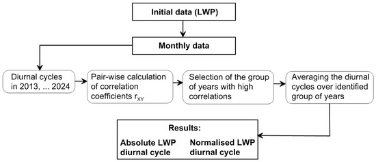
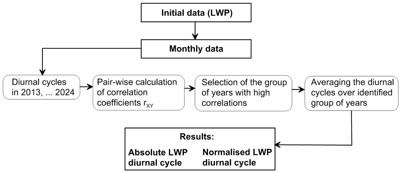
where angle brackets denote averaging over 24 h. Finally, the functions G(ti) and H(ti) are used as reliable estimates of the LWP diurnal cycle for a given month and are suitable for further analysis and comparison with data from other sources. For clarity, the algorithm is presented as a flowchart in Figure 1. The complete procedure is shown for January. The algorithm is identical for other months; however, it should be kept in mind that the number of years in the identified groups may vary for different months, as will be shown below.
Figure 1.
A flowchart of processing the monthly data. The process is repeated over all months.
4. Results
4.1. Selection of the Correlation Coefficient Threshold
Before describing the results, we will provide a few remarks regarding the choice of the correlation coefficient threshold, which must be determined before identifying groups of years with similar weather conditions that are typical for a given month. As shown in a recent study by Gnambs [18], in the case of small sample sizes, the following expression for the standard error of the correlation coefficient is recommended:
where r is the correlation coefficient, and N is the sample size. To evaluate the LWP diurnal cycle, we have chosen the 4 h time step and the corresponding 4 h averaging. This choice has been made after the extensive analysis of the initial data and numerous attempts to find the optimal sampling time. The criterion for the optimal sampling time was the ability to capture the main diurnal features and simultaneously to eliminate the noise fluctuations. Our correlation analysis method required uncorrelated measurements, so a sliding window approach, which ensures a smooth data flow but makes data points highly correlated, was not applicable. The 4 h time step means that in our case N = 6 and the correlation coefficient is statistically significant at the 98% confidence level if r > 0.75 where the value 0.75 corresponds to 3·σr. Therefore, the threshold value should not be less than 0.75. Obviously, it is better to use the highest possible threshold value to better identify years with similar weather conditions, but very high values of r are not expected in reality. Table 2 presents the results of identifying groups of years with similar conditions for the array “A” (true LWP) and for two values of the threshold r0: 0.75 and 0.8. For some months, such as January, March, July, August, November, and December, the year groups are identical for both threshold values. For some months (February, April, May, June, September) the groups overlap significantly. For October, the groups are completely different. The algorithm for selecting year groups from a matrix consisting of correlation coefficients is described in more detail in the Appendix A. It is important to note that, for each month, only a few years out of the twelve are included in the group. This result is obvious, as no one would expect the main features of LWP evolution to be clearly evident throughout the entire observation period. Without 12 years of data, it would likely be impossible to determine the main features of the LWP diurnal cycle due to the lack of correlated periods. Finally, for further analysis, we used the year groups calculated with r0 = 0.8 to retain the years with the highest r (see groups marked by crosses in Table 2).
Table 2.
Groups of years with similar weather conditions identified for different months within subset “A” using the correlation coefficient threshold values 0.75 (circles) and 0.8 (crosses).
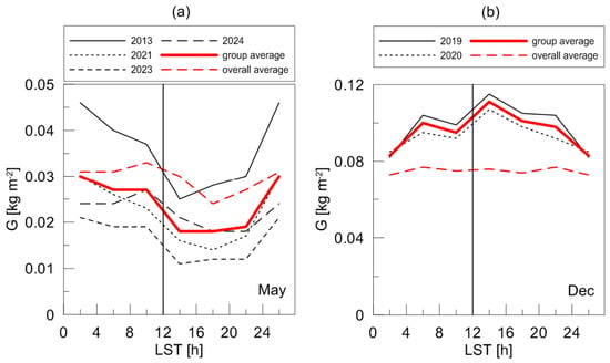
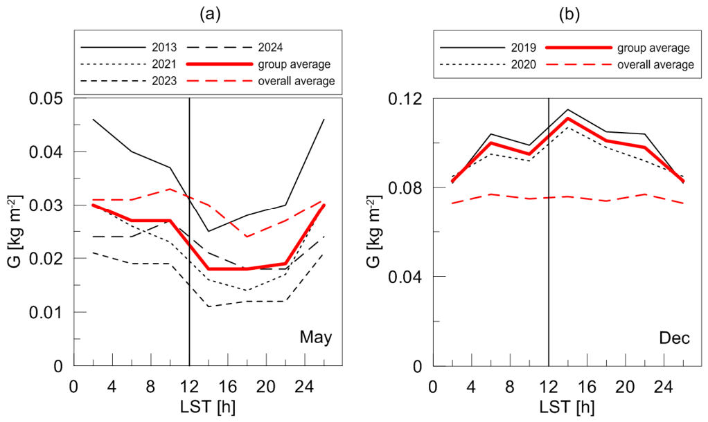
To clearly illustrate how the averaging over selected group works, we present Figure 2, which shows the diurnal cycles of the LWP relative to local solar time (LST) for May and December. It should be remembered that the errors in the calculated monthly averages are very small and therefore not visible in this and subsequent figures, as they are impossible to discern within the plot scale. The same applies to the standard deviation of the averages. As can be seen from Figure 2, the LWP values in May are significantly lower than in December due to the seasonal LWP cycle. The May group includes four years, while the December group includes only two years, indicating relatively stable weather conditions in May and variable weather conditions in December. This feature is also confirmed by the qualitative similarity between the group average and the overall average LWP diurnal cycles in May. It should be emphasised that the situation is different in December when the overall average LWP diurnal cycle does not exhibit any specific features while the group average cycle clearly shows a maximum after midday and a minimum after midnight. Obviously, the approach based on selection of the groups of years with similar diurnal patterns helps to identify the characteristic features of the LWP diurnal evolution.
Figure 2.
The diurnal cycles of LWP on the local solar time (LST) scale for May (a) and December (b) for individual years in the groups (black lines, see the legend), as well as the cycles obtained as the average value for the group and the average value for all years (red lines, see the legend). The vertical black lines mark local noon.
4.2. Diurnal Cycles of Absolute LWP Values
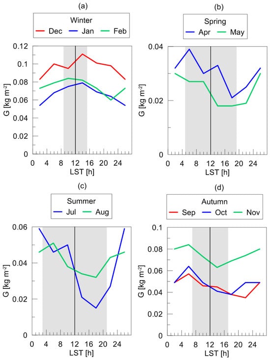
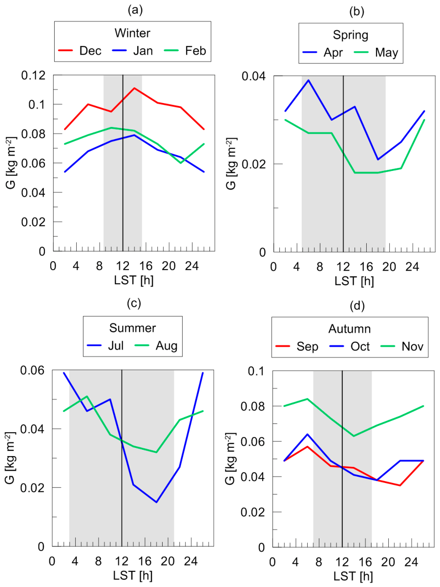
The obtained absolute diurnal cycles of the true LWP (dataset “A”, clear-sky cases not included) for individual months (except March and June, which are considered separately below) are shown in Figure 3. The results are grouped by season. The vertical black lines mark local noon, and the shaded areas show typical hours of sunshine for different seasons. The geographical point of the observations is located at 60° N; therefore, the duration of the solar illumination period varies considerably from season to season. From this figure, two types of LWP diurnal cycles can be easily distinguished. The first type applies to the winter season and is characterised by a maximum LWP between 10:00 and 14:00 LST during the short period of sunlight and a minimum at night between 22:00 LST and 02:00 LST. The second type applies to the warm seasons (spring, summer, and autumn). It is characterised by a maximum LWP around sunrise and a minimum around sunset. However, there is significant variation in the timing of the minimum, which can occur well before sunset (for example, in May, July, and November) and well after sunset (for example, in September). To conclude our discussion of Figure 3, let us note the seasonal differences in absolute LWP values. The highest LWP values are observed in autumn and winter, while the lowest are observed in spring and summer (note the different scales of the vertical axis in Figure 3).
Figure 3.
The absolute diurnal cycles of the true LWP (dataset “A”) for individual months (except March and June, see the text) grouped by season ((a–d), see the legends). The vertical black lines mark local noon. The shaded areas show typical hours of sunshine for different seasons: 15 January (a), 15 April (b), 15 July (c), and 15 October (d).
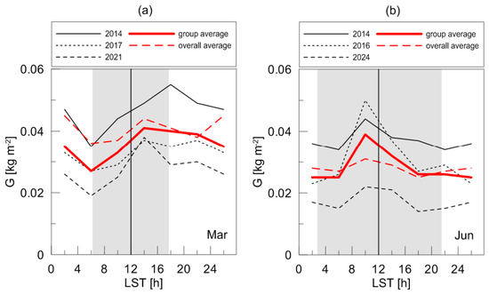
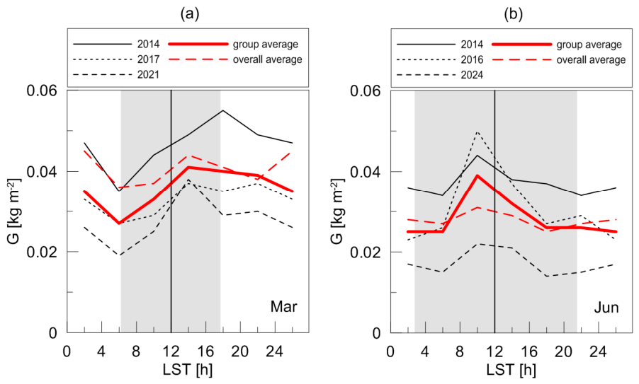
The diurnal cycles of the true LWP for March and June are shown in Figure 4. These cycles differ significantly from those in the other months discussed above. In March, the LWP values increase from dawn to afternoon and remain nearly constant in the late afternoon. At night, the LWP values decrease. One can easily see that this behaviour is the opposite of the LWP evolution in the other two spring months—April and May: LWP increases during the day instead of decreasing, and vice versa at night. In some ways, the cycle in March resembles the LWP evolution in the winter months: the difference is that the minimum shifts from midnight to dawn and the maximum shifts from noon to dusk. In June, there are no significant diurnal variations in the LWP except one distinguishable large maximum centred at 10:00. The increase in the LWP starts at about 6:00 and the decrease ends at about 18:00. Note that the sun illumination period in June is very large at the latitude 60° N where observations were carried out. We intentionally show in Figure 4 the overall average diurnal cycles along with the group average cycles. The similarity of these cycles demonstrates that the specific behaviour of LWPs during these two months is not due to random group selection but is a characteristic feature of LWP evolution.
Figure 4.
The diurnal cycles of true LWP for March (a) and June (b) for individual years in the groups (black lines, see the legend), as well as the cycles obtained as the average value for the group and the average value for all years (red lines, see the legend). The vertical black lines mark local noon. The shaded areas show the hours of solar illumination on days in the middle of the months: 15 March (a), and 15 June (b).
4.3. Normalised Diurnal Cycles of LWP
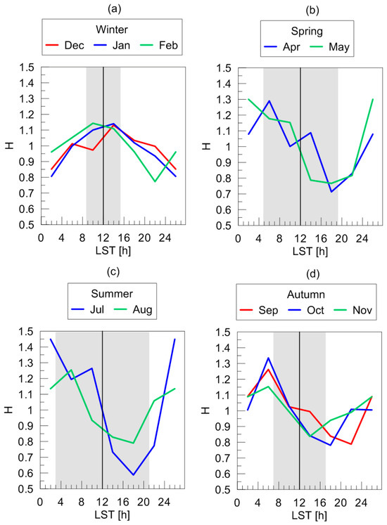
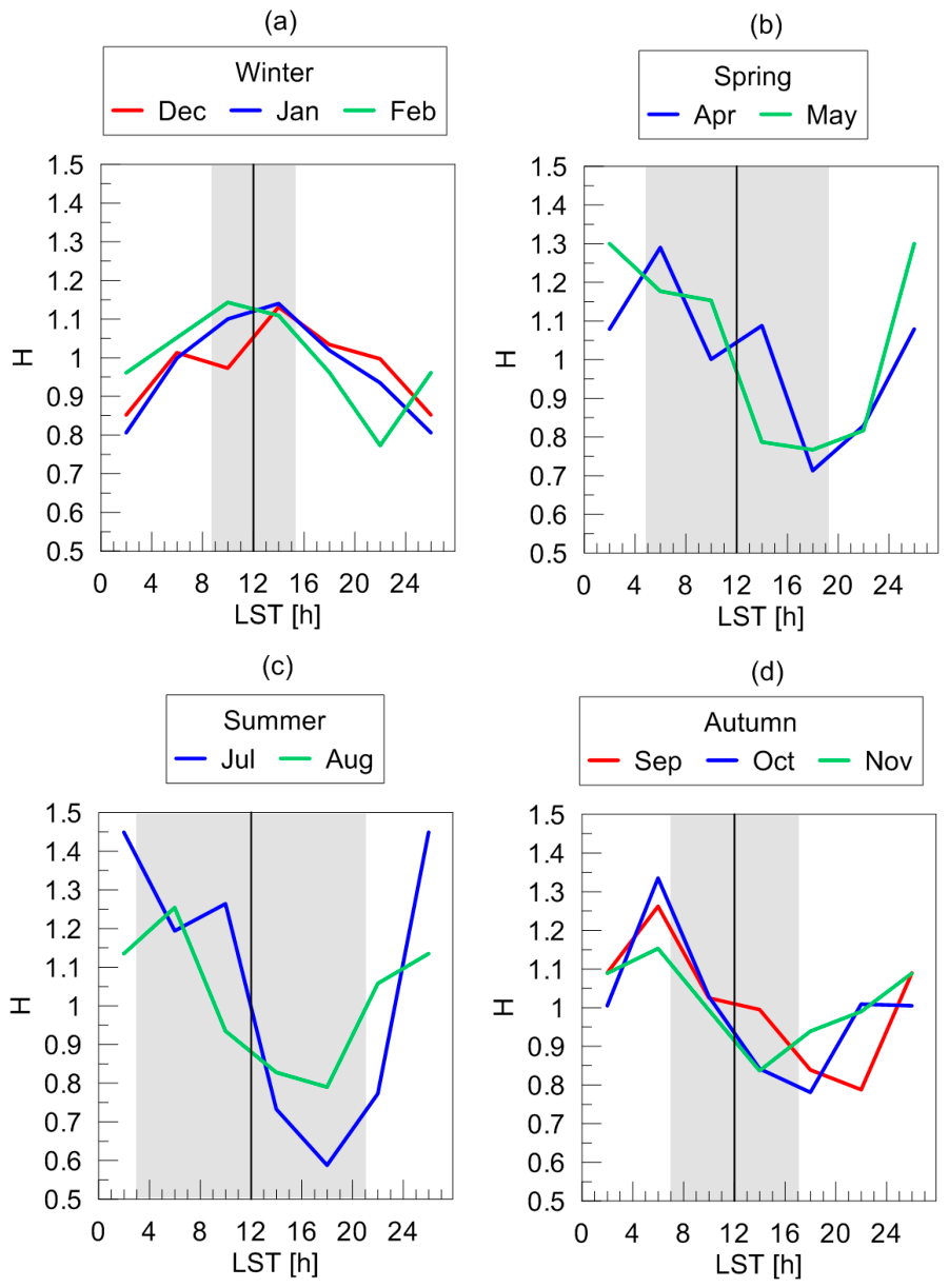
The obtained normalised diurnal cycles of the true LWP (dataset “A”, clear-sky cases not included) for individual months (except March and June, which are considered separately below) are shown in Figure 5. This figure is like Figure 3 but clearly illustrates the similarity of the LWP evolution for different months. Note the scale of the vertical axes, which allows for changes in the LWP to be shown up to 50% relative to the daily mean. Following the study by Wood et al. [1], we define the relative amplitude of the diurnal variation in the LWP as half of the difference between the maximum and minimum values, expressed as a percentage of the diurnal mean. As can be seen from Figure 5, the amplitudes are virtually identical over the three winter months, amounting to approximately 17%. In April and May, the amplitudes are larger, reaching 30%. The highest amplitude is observed in summer, in July, and exceeds 40%. In autumn, in September and October, the amplitudes are similar to those in spring, amounting to approximately 25%. In November, the amplitude is closer to the winter amplitude, equal to 15%. It is obvious that the seasonal dependence of the diurnal cycle amplitude is clearly visible. A notable feature is the good coincidence of the normalised LWP cycles for different months within a single season. Figure 5 clearly shows the similar patterns of the LWP cycle in spring, summer, and autumn, which were already noted in Figure 3: a maximum approximately at dawn, a minimum approximately at sunset, an increase at night, and a decrease during daylight hours.
Figure 5.
The normalised diurnal cycles of the true LWP (subset “A”) for individual months (except March and June, see the text) grouped by season ((a–d), see the legends). The vertical black lines represent local noon. The shaded areas show typical hours of sunshine for different seasons: 15 January (a), 15 April (b), 15 July (c), and 15 October (d).
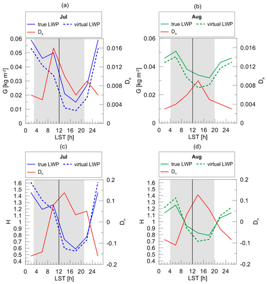
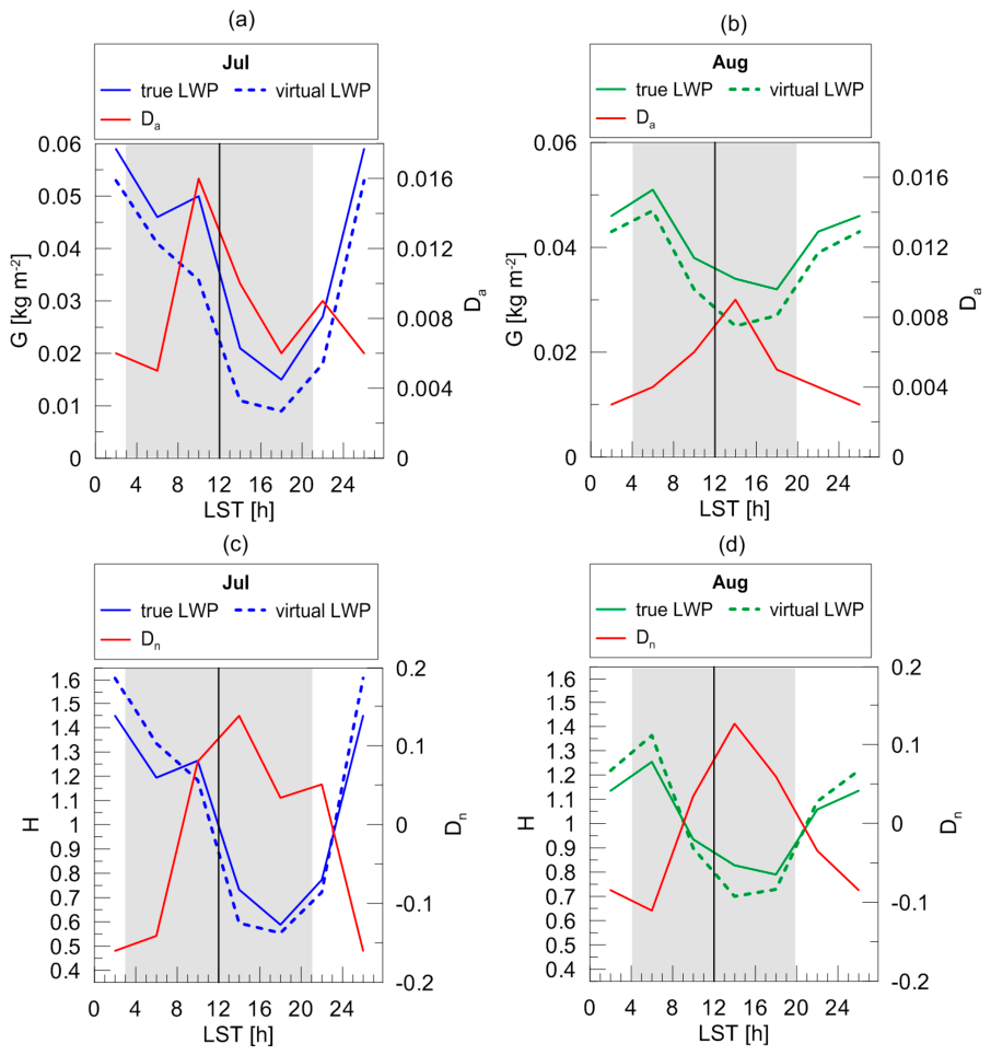
As noted above, we analyse two datasets, one containing measurements only under cloudy conditions (the so-called true LWP), and the other additionally containing measurements under clear-sky conditions with zero LWP (the so-called virtual LWP). The second dataset characterises the atmosphere as a “whole”, in other words as a more variable object. It is clear that the presence of a certain number of zero values in the dataset “B” leads to a decrease in LWP values throughout the absolute diurnal cycle. This effect is illustrated in Figure 6a,b, where the absolute diurnal cycles of true and virtual LWPs are shown for July and August. The diurnal evolution of the difference between the true and the virtual LWP is also shown, which qualitatively characterises the frequency of clear-sky episodes. One can see that the clear-sky episodes were most frequent approximately 2 h before local noon in July and approximately 2 h after local noon in August.
Figure 6.
The absolute (a,b) and the normalised (c,d) diurnal cycles of the true LWP (dataset “A”) and virtual LWP (dataset “B”) for July and August. The vertical black lines mark local noon. The shaded areas show the hours of solar illumination on days in the middle of the months: 15 July (a), and 15 August (b). The red lines show the difference between the true and virtual LWP values for absolute cycles (Da) and for normalised cycles (Dn); see the right vertical axes.
Although the absolute diurnal cycles of the true and virtual LWP differ across all twelve months, the normalised diurnal cycles of the true and virtual LWP are qualitatively and quantitatively very similar in all months except July and August. Therefore, Figure 6c,d shows the normalised diurnal cycles of true and virtual LWPs for these two months. It is clearly evident that the normalised cycle amplitude for the true LWP is significantly smaller than the normalised cycle amplitude for the virtual LWP. In June, the difference can reach 15%, and in August, 10% (see the red curves in the figure).
4.4. Diurnal Cycle Parameters, Approximations and Uncertainty Estimation
Given the strong seasonal variability of the LWP values and of their diurnal evolution, it makes sense to focus on the key parameters of the normalised diurnal cycle for each season. The results discussed above lead to the conclusion that to describe the diurnal cycle, it is sufficient to consider three key parameters: the time of maximum tmax, the time of minimum tmin and the amplitude A. In our study, we take standard deviations of the average values of these parameters σmax, σmin and σA as the measures of their uncertainty. To better estimate the standard deviations for each season, we use the data from all months in the season and from all years in the selected groups. Let us consider two examples. As it can be seen from Table 2, to calculate the standard deviations for winter, we take the data for December in 2019 and 2020, for January in 2013 and 2015, and for February in 2014 and 2016. So, we have six data values for each key parameter. For autumn, we take the data for September in 2017, 2018, 2019, and 2022, for October in 2018 and 2021, and for November in 2020, 2021, 2022, and 2023. As a result, we have 10 data values for each key parameter in autumn. We obtain the standard deviation of the mean values by dividing the standard deviation of all samples by the square root of the number of samples. The uncertainty of the original data (monthly average LWP values) is negligible and is not taken into account. However, for time moments of the LWP minimum and maximum, we consider half a time step of the time scale as a measurement error as it is quite large (2 h).
Table 3 presents the obtained mean values of the key parameters and their standard deviations, which we use as an estimate of their uncertainty. One can see that this Table summarises the results discussed above and confirms the preliminary conclusions. The diurnal cycles are similar in warm seasons with the maximum LWP in the early morning at 03:00–06:00 LST and the minimum LWP in the evening at 16:00–19:00 LST. The LWP evolution in the cold winter season differs considerably, having a maximum at noon and a minimum at midnight. The uncertainty of the obtained time values is in the range from 1 h to 1.5 h. The relative amplitude of the diurnal cycle is large in summer, reaching 35%, and small in winter (about 16%), with intermediate values in spring and in autumn (22–29%). The uncertainty of the obtained values of the amplitude is about 2% for all seasons except summer when it is significantly larger and reaches 9%.
Table 3.
Average parameters of the diurnal cycle of LWP: the time of LWP minimum tmin, the time of LWP maximum tmax, and the amplitude A. Time is given in hours LST and in decimal notation.
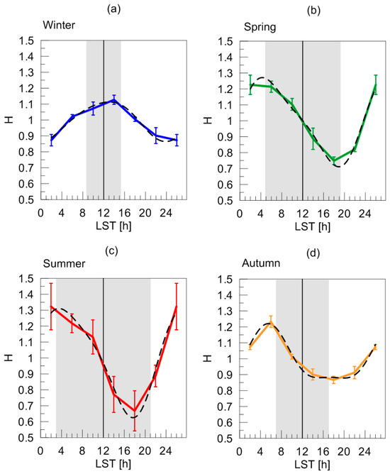
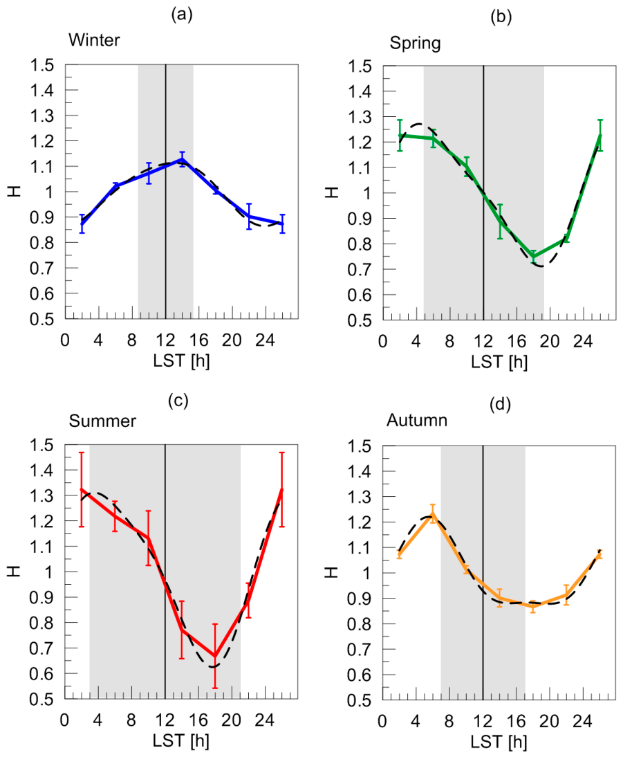
Figure 7 shows the average normalised LWP diurnal cycles H(t) for all seasons computed based on the data from all months in the season and from all years in the selected groups. We used the same approach as for deriving the parameters tmin, tmax and A discussed above. Additionally, the following approximation is shown for each season:
where A24 is the relative amplitude (dimensionless) and b24 is the phase (hours in decimal notation) of the diurnal (24 h) mode, while A12 and b12 are the relative amplitude and the phase of the semi-diurnal (12 h) mode. We have chosen this approximation based on the results of the study by Cairns [19], who investigated the diurnal variability of the cloud amount from ISCCP (International Satellite Cloud Climatology project) data using the principal component analysis. It was found that the global average diurnal cycle was almost the same in all seasons with the first and second principal components being close to the diurnal cycle in seasonal cloud amount and the third and fourth principal components being close to the semi-diurnal cycle in seasonal cloud amount. Therefore, we used harmonic functions representing both of these components. The values of the parameters of the approximation as well as the coefficient of determination R2 are presented in Table 4 for each season.
Figure 7.
The average normalised diurnal cycles of the true LWP for all seasons (plots (a−d), coloured lines). Error bars present the standard deviation of the LWP mean values at different moments of time. The black dashed lines show the two-mode sinusoidal approximations. The vertical black lines mark local noon. The shaded areas show typical hours of sunshine for different seasons: 15 January (a), 15 April (b), 15 July (c), and 15 October (d).
Table 4.
Parameters of the approximations of the normalised diurnal cycle of LWP for different seasons.
It is clearly seen that the two-mode sinusoidal approximations agree very well with the original diurnal cycles for each season. The coefficients of determination are in the range of 0.96–0.98, meaning that the approximations explain almost all the diurnal variability of the LWP. The amplitudes of the diurnal and semi-diurnal cycles are maximal in summer and minimal in winter. The approximations for the three warm seasons (spring, summer, and autumn) have very similar phases b24, differing by less than one hour. In contrast, the phase b24 in winter is shifted relative to the phases in the other seasons by approximately 6.5–7 h. This fact demonstrates that the LWP maximum is shifted from midday in winter to dawn in the other seasons. In conclusion, it is worth noting that although a polynomial approximation may be useful for practical purposes, we prefer to focus on the two-mode sinusoidal approximation, which has a clear physical meaning.
5. Discussion
5.1. Comparison with the Results of Other Ground-Based Microwave Measurements of LWP
Results of the assessment of the LWP diurnal evolution using ground-based microwave instruments are not numerous, especially in coastal zones. Fairall et al. [20] reported the average LWP diurnal cycle of stratocumulus clouds, which had been derived from 19-day observations in June–July 1987 using a three-channel (20.6, 31.65 and 90.0 GHz) microwave radiometer located on San Nicolas Island near Los Angeles. The accuracy of the LWP retrievals was declared as 20%. Clear-sky conditions were not included in the statistics. The diurnal variations of LWPs were found to be very large with the maximum of approximately 0.135 kg m−2 in the morning and a minimum of approximately 0.025 kg m−2 in the evening. Thus, the amplitude was about 60–70% of the mean value. Despite these measurements having been carried out in a climate zone that differs from the climate zone of the Baltic region, the obtained result is similar to the LWP cycle found in our study for the spring, summer and autumn periods, except that in the present study the LWP maximum value and the LWP amplitude are lower by a factor of two or more. We are not aware of any papers describing microwave measurements of LWPs in coastal zones with a climate similar to that of the Baltic region.
As far as the inland microwave measurements are concerned, we would like first of all to mention a series of papers by Cossu at al. [15] and Hocke et al. [21,22], who analysed the diurnal cycle of cloud LWPs and cloud fractions over Bern, Switzerland, based on long-term ground-based microwave observations by the two-channel (21.4 GHz and 31.5 GHz) TROWARA instrument (TROpospheric WAter RAdiometer). Similar to our study, the upper threshold of 0.4 kg m−2 was used for the LWP and only non-raining clouds were considered. The diurnal cycle of the LWP has been shown to vary from month to month, with relative amplitudes of 15 to 25% reached, especially in October, November, and January. This result is opposite to our result, which shows the maximum relative amplitude in the summer months, despite the fact that the maximum absolute values of the LWP are observed in winter. Hocke et al. [22] reported that the annual mean of the diurnal cycle shows a minimum around −10%, which occurs around midday. At night, a relative maximum of 9% is reached around 03:00 local time. Since we found markedly different diurnal cycles of LWPs across seasons (see Table 3), we do not estimate the annual mean of the cycle. However, it should be noted that we obtained amplitudes that are significantly larger than in the study by Hocke et al. [22]. Furthermore, we show the minimum during spring, summer and autumn not around noon, but at 16:00–19:00 local solar time. Regarding the time of the maximum, our estimate for spring, summer and autumn is slightly biased towards the morning hours compared to the result obtained by Hocke et al. [22].
The issue of the variability of the LWP diurnal cycle requires special attention, since we found cycles in March and June that differ significantly from cycles in other months. Cossu et al. [15] investigated the diurnal cycle of cloud fraction (CF) and have suggested that seasonality does not seem to be the only driver of the diurnal cycle, since a strong intraseasonal variability is present, as months belonging to the same season do not always exhibit a similar behaviour. For example, Cossu et al. [15] found large differences between the CF cycles during consecutive months January/February, June/July and September/October and assumed that these differences may be caused by multiple processes (local thermodynamic parameters, radiation fluxes, large-scale atmospheric circulation, turbulent fluxes, atmospheric moist convection, etc.), which influence the cloud evolution. It is worth noting that the time moments of minimum and maximum of the sinusoidal approximation of the 10-year mean CF diurnal cycle in the work by Cossu et al. [15] are similar to the corresponding parameters obtained in our study for the LWP diurnal cycle in all seasons except winter. It is worth noting also that when the CF and LWP diurnal cycles have the same phase with maxima in the early morning and minima around 15 h LST, this suggests that the diurnal cycle is mainly driven by solar heating [23].
Other examples of the inland microwave measurements of LWPs can be found in the review by Xu [24], who summarised the achievements of remote sensing of atmospheric profiles and cloud properties using ground-based microwave measurements in central China; in particular, the results of assessing the diurnal cycle of LWPs at different locations. According to the studies of Xu et al. [25,26], the diurnal cycle of the cloud occurrence frequency (COF) of low and middle clouds differs significantly during the summer period on the eastern Tibetan Plateau and in central China. Furthermore, the differences were also observed in the LWP diurnal cycle. In central China, for all types of non-precipitating clouds, the LWP is relatively high during the day and low at night [25]. On the Tibetan Plateau, the situation is reversed: the maximum LWP is observed at night and the minimum is observed during the day [26]. The LWP cycle observed in central China in summer is somewhat similar to the LWP cycle we obtained under winter conditions, where we observe smooth changes in LWP values over time with the maximum at about noon. It is very important to note that the LWP values obtained by Xu et al. [25,26] in the diurnal cycles reach 0.2–0.5 kg m−2 and are therefore significantly larger than the LWP values in our study. Xu et al. [25,26] likely did not apply any LWP upper limits during the data quality assessment and data selection process. Therefore, we cannot consider the comparison between our results and the results from China to be rigorous and fully valid.
5.2. Comparison with the Results of Space-Based Microwave Measurements of LWP
Most information on the LWP diurnal evolution has been obtained from space-based microwave observations, but only over the oceans. In contrast, the space-based LWP measurements using instruments operating in the visible and near-infrared spectral ranges and recording reflected solar radiation also provide information over land, but only under solar illumination conditions. Thus, the advantage of microwave measurements of LWPs from space is the ability to derive the 24 h dynamics of LWPs.
The diurnal cycle of liquid water paths over the subtropical and tropical oceans has been examined by Wood et al. [1] using two complete years of TMI (Tropical Rainfall Measuring Mission Microwave Imager) satellite microwave radiometer data. Random retrieval errors in LWPs were estimated to be 0.025 kg m−2 with a small systematic error of 0.005 kg m−2. The normalised amplitudes of the diurnal cycle were found to be greatest (0.15–0.30) in the low cloud regions and close to the island landmasses. Wood et al. [1] have suggested that they may be accentuated by the effect of sea/land breeze triggering of deep convection. It should be noted that the observation point in our study is located in close proximity to the coastline of the Gulf of Finland, and therefore the diurnal cycle of the LWP may also be influenced by breeze circulation. Although we obtained an estimate of the evolution of the LWP at a high latitude, there is good agreement between the amplitude values obtained in our study and those obtained in the study by Wood et al. [1]. Furthermore, there is good agreement in the seasonal dependence of the amplitude of the LWP diurnal cycle, with both studies reporting larger amplitudes in summer and smaller amplitudes in winter. It is also worth noting that the study by Wood et al. [1] showed a morning peak in the LWP at 02–05 LST, while our study showed a warm-season morning peak at 04–06 LST. The study by Wood et al. [1] demonstrated that the sinusoidal fit provides an adequate model of the diurnal evolution in the LWP with some deviations near 00 LST. It was suggested that these deviations do not impair the usefulness of the sinusoidal model but indicate that there may be a somewhat more complex diurnal cycle, possibly related to local variations. In our study, we obtained similar results with the sinusoidal fit of the LWP diurnal cycle; however, the deviations appear at different times during the night.
5.3. Comparison with the Results of Space-Based Measurements of LWP by the SEVIRI Instrument
The SEVIRI instrument operates in the visible and near-infrared spectral ranges and records reflected solar radiation. As a result, as mentioned above, it provides the information on LWPs both over land and water surfaces, however only under solar illumination conditions when the solar zenith angle is smaller than 72°, i.e., covering the period between approximately one hour after sunrise and one hour before sunset. Therefore, the derivation of the complete 24 h LWP cycle from the SEVIRI measurements is not possible.
The LWP evolution during sunlight hours obtained by the SEVIRI instrument over the observational site of St. Petersburg University near the coastline of the Gulf of Finland was compared to the LWP evolution measured by the ground-based microwave instrument HATPRO during the period December 2012–November 2014 [10]. Over 7 months (February–May and August–October), the SEVIRI and the HATPRO instruments revealed similar diurnal variations in the LWP, while considerable discrepancies between the diurnal variations obtained by the two instruments were detected in June and July. Some common features were noticed for the summer months: the SEVIRI instrument detected two maxima—the higher one at about noon and the lower one in the evening, probably due to convection processes. For other months it was difficult to propose any simple explanations of the LWP cycle and to conclude whether these cycles were typical for the considered months or not. These previous results, in particular, motivated us to conduct this study, which aimed to evaluate LWP cycles that are truly typical for our measurement point. Since a detailed comparative study involving 12-year measurements by the ground-based HATPRO microwave radiometer and by the space-based SEVIRI instrument is beyond the scope of the present work, below we present only a short overview of the SEVIRI data relevant to the LWP evolution.
Diurnal cycles of LWPs over European land and sea areas during summer in various climate regions were estimated by Roebeling et al. [27] based on satellite measurements of reflected solar radiation made by the SEVIRI instrument. Distinct differences were demonstrated between the time of maximum LWP values over land and ocean. Over oceans, the LWP maximum was detected in early morning observations while over land the daytime maximum was generally found after local solar noon. Applying this finding to our results, we can conclude that most of the warm period at the observation point near the Gulf of Finland is characterised by marine-type clouds with an LWP maximum before and just after sunrise. However, in March and June the situation is reversed and continental-type clouds predominate with a maximum in the LWP around midday. In this case, the evolution of the LWP is determined by convective clouds, which respond strongly to the diurnal cycle of surface heating. In the morning, the surface begins to warm up, and convective processes begin to develop, leading to the strongest convection, as a rule, in the afternoon. At night, the land surface cools, and convective cloud systems disappear. It should be noted that Roebeling et al. [27] noted significant differences in the timing of the LWP maximum between different climatic regions. For example, convection in continental Europe is weaker than in the land area of the Mediterranean, due to the less pronounced heating of the surface during the day.
The study by Roebeling and Meijgaard [28] is somewhat similar to the study by Roebeling et al. [27] but focuses on the cloud amount and cloud condensed water path (CWP), which is the sum of the LWP and ice water path (IWP). They found that over most of the oceanic and coastal areas of Europe, the time of the daily maximum of the CWP occurs in the morning, while over land this maximum occurs after local solar noon. In this respect, the evolution of the CWP is similar to the evolution of the LWP obtained in the study by Roebeling et al. [27]. The location of the microwave observations in our study can be classified as coastal; therefore, it is not surprising that our results agree well with independent estimations of the LWP cycle under similar climatic conditions.
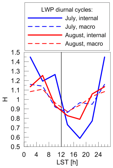
In our study, we used the same approach to data classification as in the study by Kniffka et al. [29], who examined the LWP values obtained from the SEVIRI space-based measurements. Namely, we separated measurements under cloudy conditions only from measurements under both cloudy and clear-sky conditions. As noted above, this approach helps to analyse separately the internal properties of clouds and the properties of the atmosphere as a whole as well. Kniffka et al. [29] have suggested that the diurnal cycle of LWPs is generated either by internal fluctuations of LWPs in the cloud field or by macroscopic variations in cloud cover, i.e., the absence or presence of clouds in this respect. They partitioned the mean diurnal cycle into components of these two parts. The internal fraction was determined by averaging over all pixels with an LWP greater than zero. Macroscopic variation in cloud cover was estimated by calculating and comparing the number of pixels in the space-borne measurements with and without clouds. In our study, we followed the concept of “virtual LWP”, which allows estimating the macroscopic part of the LWP diurnal cycle without assessment of cloud cover. The overall normalised diurnal cycle of the LWP is equal to the cycle of the virtual LWP and can be expressed as follows:
where δ denotes the deviation from unity, and the indices “true” and “macro” denote the contribution of internal and macroscopic processes to the overall cycle described by the index “virt”. As a result, the normalised diurnal cycle determined by macroscopic processes can be obtained using the following expression:
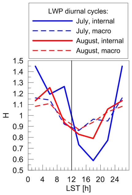
The quantity δHtrue(t) − δHvirt(t) for July and August is shown in Figure 6 and was discussed above. Additionally, to give a clear illustration of the diurnal cycle determined by macroscopic processes, we plot this cycle together with the intrinsic variability in LWPs in Figure 8, which is similar to Figure 10b in the paper by Kniffka et al. [29].
Figure 8.
The average normalised diurnal cycles of LWP corresponding to two mechanisms of the cloud evolution: “internal” and “macroscopic” (see the legend and the text). The vertical black line marks local noon.
Despite the differences in geographic location and climate between our measurements and those reported by Kniffka et al. [29], there are three common features in the evolution of LWPs. First, the variability caused by macroscopic processes (i.e., cloud fraction) is noticeably lower than the variability caused by internal processes. Recall that for months other than July and August, our study shows that the contribution of macroscopic processes is negligibly small, so we do not demonstrate it. Second, the minimum of the so-called “macroscopic” cycle is shifted toward noon relative to the minimum of the internal cycle. Third, the qualitative behaviour of both the “internal” and “macro” cycles obtained in the present study and in the study of Kniffka et al. [29] is similar.
6. Summary and Conclusions
The liquid water path is an important cloud parameter. The information on its long-term and short-term variability is essential for a wide spectrum of atmospheric studies including climatological ones. In this paper, we presented for the first time the results of the estimations of the LWP diurnal cycle based on the 12-year ground-based microwave measurements using the HATPRO radiometer near the coastline of the Gulf of Finland (59.88107° N, 29.82597° E).
All estimations have been made for an LWP smaller than 0.4 kg m−2. This value has been reported earlier as a threshold LWP between non-rainy and rainy atmospheres and the higher values of the retrieved LWP may contain large errors. Two different sampling datasets were used that include the so-called true and virtual LWP values. True LWP values (6,088,782 samples) correspond to measurements under cloudy conditions only while virtual LWP values (7,140,234 samples) correspond to measurements under both cloudy and clear-sky conditions; that is, a virtual LWP value can be zero. A joint analysis of these quantities allowed us to separate the contributions of internal cloud processes and external macroscopic processes to the LWP diurnal cycle.
We used a unique approach to identifying time intervals characterised by similar meteorological conditions and suitable for inferring the diurnal evolution of LWPs. This approach is based on an analysis of the correlation coefficients between monthly average LWP diurnal cycles corresponding to different years and helped greatly to capture the typical diurnal cycles, especially in the winter months. All correlation coefficients for the LWP diurnal cycles during the periods with similar meteorological conditions exceed 0.8.
The main results of the LWP diurnal cycle assessment for 2013–2024 are as follows:
- (1)
- Two types of diurnal cycles of LWP were identified, one of which was observed in winter and the other in spring, summer and autumn. Two months (March and June) were characterised by specific diurnal cycles. The highest LWP values are observed in autumn and winter, while the lowest are observed in spring and summer.
- (2)
- The cycle that applies to the winter season is characterised by a maximum LWP between 10:00 and 14:00 LST during the short period of sunlight and a minimum at night between 22:00 and 02:00 LST. The cycle that applies to the warm seasons (spring, summer, and autumn) is characterised by a maximum LWP around sunrise and a minimum around sunset. However, there is significant variation in the timing of the minimum, which can occur well before sunset (for example, in May, July, and November) and well after sunset (for example, in September).
- (3)
- In March, LWP values increase from dawn to afternoon and remain nearly constant in the late afternoon. At night, the LWP values decrease. In some ways, the cycle in March resembles the LWP evolution in the winter months: the difference is that the minimum shifts from midnight to dawn and the maximum shifts from noon to dusk. In June, there are no significant diurnal variations in the LWP except one distinguishable large maximum centred at 10:00 LST. The increase in LWP starts at about 6:00 LST and the decrease ends at about 18:00 LST.
- (4)
- The amplitude of the normalised LWP cycle has a clear seasonal dependence with a minimum of 16.4 ± 2.5% in winter and a maximum of 35.6 ± 9.3% in summer. The average time moments of the LWP minima and maxima during different seasons are given in a tabular form with an accuracy better than 1.5 h.
- (5)
- The two-mode (diurnal and semi-diurnal) sinusoidal approximation of the normalised LWP diurnal cycle works very well for all seasons with the coefficients of determination in the range of 0.96–0.98, meaning that the approximations explain almost all the diurnal variability in the LWP. The phase of the 24-hour mode of the winter approximation is shifted relative to the 24 h phases in the other seasons by approximately 6.5–7 h.
- (6)
- The variability in the LWP caused by macroscopic processes (i.e., cloud fraction) is noticeably lower than the variability caused by internal cloud processes. For months other than July and August, the contribution of macroscopic processes is negligible. In July and August, the time of minimum of the “macroscopic” part of the LWP cycle is shifted toward noon relative to the time of minimum of the cloud “internal” LWP cycle.
- (7)
- Comparative analysis of the obtained LWP diurnal cycles and the LWP cycles detected using different ground-based and space-borne instruments worldwide has shown that the observed LWP cycle in spring, summer and autumn is similar to the cycle of the marine stratocumulus clouds. This conclusion is not surprising since the observational point is located near the coastline of the Gulf of Finland and the meteorological conditions are determined by the influence of the Baltic Sea. In winter and also during March and June, the LWP cycle can be attributed to the continental type.
The obtained results can be useful as important constraints for different models that contain simulations of the LWP diurnal cycle in the Baltic Sea region.
Author Contributions
V.S.K.: conceptualisation; investigation; formal analysis; data processing; funding acquisition; writing—original draft. D.V.I.: investigation; formal analysis; methodology. M.V.M.: investigation; formal analysis; methodology. All authors have read and agreed to the published version of the manuscript.
Funding
The work was supported by the Russian Science Foundation (grant no. 24-27-00016, https://rscf.ru/project/24-27-00016/, accessed on 1 April 2026).
Institutional Review Board Statement
Not applicable.
Informed Consent Statement
Not applicable.
Data Availability Statement
Dataset available on request from the authors.
Acknowledgments
The operation of the RPG-HATPRO instrument was provided by the Research Centre GEOMODEL of St. Petersburg State University (https://researchpark.spbu.ru/index.php/en/geomodel-eng, last access: 23 December 2025).
Conflicts of Interest
The authors declare no conflict of interest.
Appendix A. Matrices of Correlation Coefficients and Selection of Year Groups for Averaging of LWP
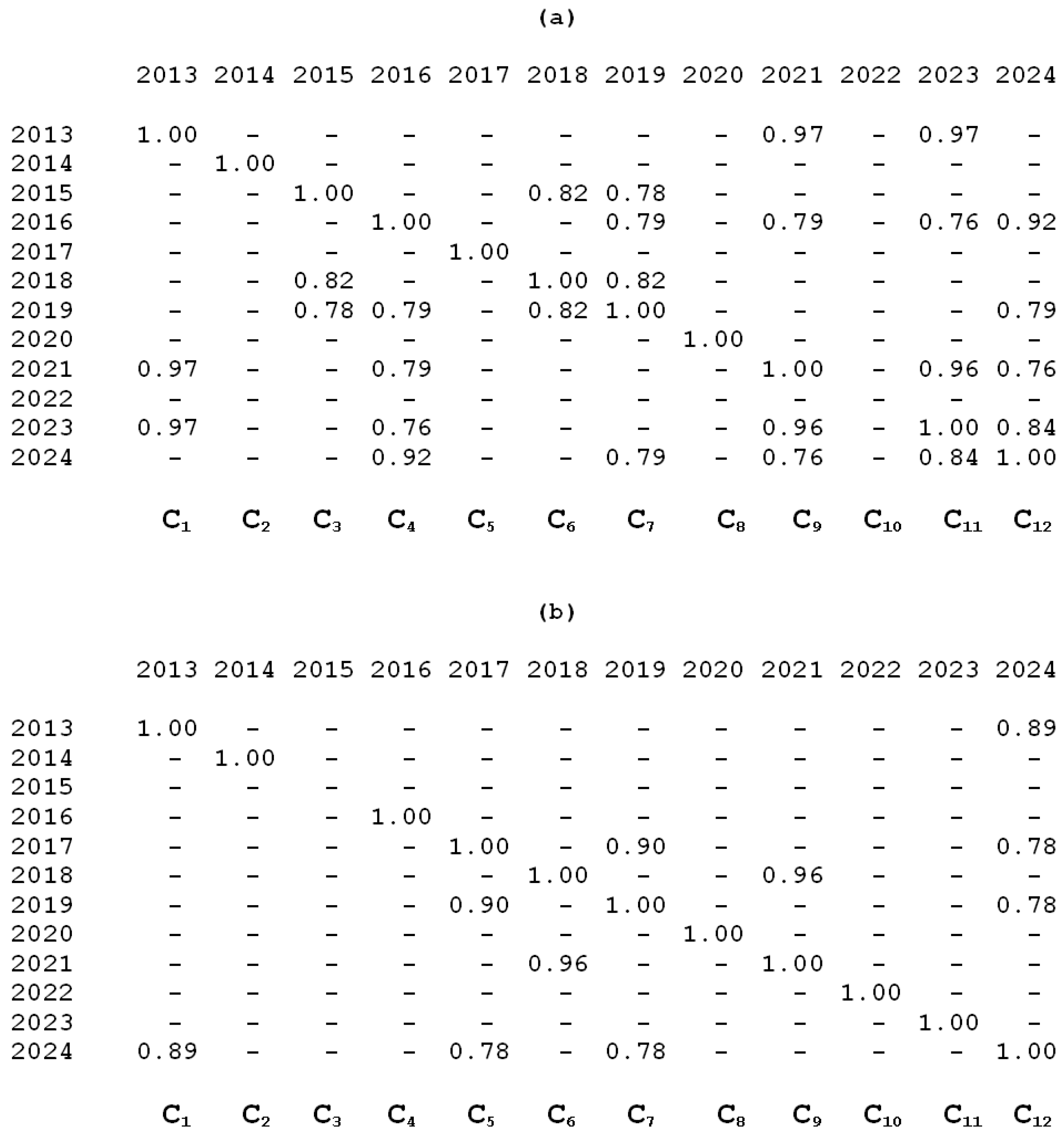
In this appendix, we provide a brief explanation of the algorithm for selecting year groups from matrices containing correlation coefficients r. Let us consider two examples shown in Figure A1, where, for simplicity, correlation coefficients below the 0.75 threshold have been omitted and replaced with hyphens. The first example concerns calculations for May. It can be seen that the largest number of matrix elements in a group (in a matrix column) exceeding the threshold of 0.75 is five and there are five such groups: C4, C7, C9, C11 and C12. For simplicity, the diagonal elements with r = 1 are also taken into account. For averaging the daily cycles of the LWP, the C11 group should be chosen, since the sum of the correlation coefficients in this group is higher than in other groups. Let us consider the situation with the threshold value of 0.8. In this case the largest number of matrix elements in a group exceeding the threshold of 0.8 is four and there is only one such group: C11. Although the selected matrix column (C11) is the same for both thresholds, in the second case the year 2016 is excluded from the calculations, leaving 2013, 2021, 2023 and 2024.
The second example concerns calculations for October. The largest number of matrix elements in a group exceeding the threshold of 0.75 is four and there is one such group: C12. Therefore, in case of the 0.75 threshold, this group should be chosen for averaging the daily cycles of the LWP. For the 0.8 threshold, the largest number of matrix elements exceeding the threshold is only two and there are six such groups: C1, C5, C6, C7, C9, and C12. For averaging the daily cycles of LWP, the group C6 or the equivalent group C9 should be chosen, since the sum of the correlation coefficients in these groups is higher than in other groups. As a result, averaging will be performed over two years: 2018 and 2021.
Figure A1.
Correlation coefficient matrices for the LWP diurnal cycle in May (a) and October (b). Rows and columns are labelled with corresponding year numbers. Letters “C” with subscripts denote matrix columns as groups. Correlation coefficients below the threshold of 0.75 are omitted and replaced with hyphens.
References
- Wood, R.; Bretherton, C.S.; Hartmann, D.L. Diurnal cycle of liquid water path over the subtropical and tropical oceans. Geophys. Res. Lett. 2002, 29, 2092. [Google Scholar] [CrossRef] [Scilit]
- Kurowski, M.J.; Lebsock, M.D.; Smalley, K.M. The diurnal susceptibility of subtropical clouds to aerosols. Atmos. Chem. Phys. 2025, 25, 15329–15342. [Google Scholar] [CrossRef] [Scilit]
- Aerenson, T.; McCoy, D.; Elsaesser, G.; Wu, J.; Nugent, J.M.; Brown, H.; Mikkelsen, A.; Zelinka, M.D. Global models predict clouds at the wrong time of day: Does it matter for radiation and climate? Sci. Adv. 2025, 11, eady3236. [Google Scholar] [CrossRef] [Scilit]
- Webb, M.J.; Lock, A.P.; Bodas-Salcedo, A.; Bony, S.; Cole, J.N.S.; Koshiro, T.; Kawai, H.; Lacagnina, C.; Selten, F.M.; Roehrig, R.; et al. The diurnal cycle of marine cloud feedback in climate models. Clim. Dyn. 2015, 44, 1419–1436. [Google Scholar] [CrossRef] [Scilit]
- Smalley, K.M.; Lebsock, M.D.; Eastman, R. Diurnal patterns in the observed cloud liquid water path response to droplet number perturbations. Geophys. Res. Lett. 2024, 51, e2023GL107323. [Google Scholar] [CrossRef] [Scilit]
- Loehnert, U.; Crewell, S. Accuracy of cloud liquid water path from ground-based microwave radiometry. 1. Dependency on cloud model statistics. Radio Sci. 2003, 38, 8041. [Google Scholar] [CrossRef] [Scilit]
- Crewell, S.; Loehnert, U. Accuracy of cloud liquid water path from ground-based microwave radiometry. 2. Sensor accuracy and synergy. Radio Sci. 2003, 38, 8042. [Google Scholar] [CrossRef] [Scilit]
- Rose, T.; Crewell, S.; Löhnert, U.; Simmer, C. A Network Suitable Microwave Radiometer for Operational Monitoring of the Cloudy Atmosphere. Atmos. Res. 2005, 75, 183–200. [Google Scholar] [CrossRef] [Scilit]
- Böck, T.; Löffler, M.; Marke, T.; Pospichal, B.; Knist, C.; Löhnert, U. Instrument uncertainties of network-suitable ground-based microwave radiometers: Overview, quantification, and mitigation strategies. Atmos. Meas. Tech. 2025, 18, 6251–6270. [Google Scholar] [CrossRef] [Scilit]
- Kostsov, V.S.; Kniffka, A.; Ionov, D.V. Cloud liquid water path in the sub-Arctic region of Europe as derived from ground-based and space-borne remote observations. Atmos. Meas. Tech. 2018, 11, 5439–5460. [Google Scholar] [CrossRef] [Scilit]
- Kostsov, V.S.; Kniffka, A.; Stengel, M.; Ionov, D.V. Cross-comparison of cloud liquid water path derived from observations by two space-borne and one ground-based instrument in northern Europe. Atmos. Meas. Tech. 2019, 12, 5927–5946. [Google Scholar] [CrossRef] [Scilit]
- Kostsov, V.S.; Makarova, M.V. Trends of Liquid Water Path of Non-Raining Clouds as Derived from Long-Term Ground-Based Microwave Measurements near the Gulf of Finland. Meteorology 2025, 4, 19. [Google Scholar] [CrossRef] [Scilit]
- Kostsov, V.S.; Ionov, D.V.; Biryukov, E.Y.; Zaitsev, N.A. Cross-validation of two liquid water path retrieval algorithms applied to ground-based microwave radiation measurements by the RPG-HATPRO instrument. Int. J. Remote Sens. 2018, 39, 1321–1342. [Google Scholar] [CrossRef] [Scilit]
- Mätzler, C.; Morland, J. Refined Physical Retrieval of Integrated Water Vapor and Cloud Liquid for Microwave Radiometer Data. IEEE Trans. Geosci. Remote Sens. 2009, 47, 1585–1594. [Google Scholar] [CrossRef]
- Cossu, F.; Hocke, K.; Mätzler, C. A 10-Year Cloud Fraction Climatology of Liquid Water Clouds over Bern Observed by a Ground-Based Microwave Radiometer. Remote Sens. 2015, 7, 7768–7784. [Google Scholar] [CrossRef] [Scilit]
- Mätzler, C. Ground-Based Observations of Atmospheric Radiation at 5, 10, 21, 35, and 94 GHz. Radio Sci. 1992, 27, 403–415. [Google Scholar] [CrossRef] [Scilit]
- Kostsov, V.S.; Ionov, D.V.; Andryukova, A.B. Estimation of Statistical Characteristics of Cloud Liquid Water Path over the Land Area and Water Bodies in the Baltic Sea Region and Northwest Russia Based on the SEVIRI Satellite Instrument Data. Izv. Atmos. Ocean. Phys. 2025, 61, 597–615. [Google Scholar] [CrossRef] [Scilit]
- Gnambs, T. A Brief Note on the Standard Error of the Pearson Correlation. Collabra Psychol. 2023, 9, 87615. [Google Scholar] [CrossRef] [Scilit]
- Cairns, B. Diurnal variations of cloud from ISCCP data. Atmos. Res. 1995, 37, 133–146. [Google Scholar] [CrossRef] [Scilit]
- Fairall, C.W.; Hare, J.E.; Snider, J.B. An eight-month sample of marine stratocumulus cloud fraction, albedo, and integrated liquid water. J. Clim. 1990, 3, 847–863. [Google Scholar] [CrossRef] [Scilit]
- Hocke, K.; Navas-Guzmán, F.; Cossu, F.; Mätzler, C. Cloud Fraction of Liquid Water Clouds above Switzerland over the Last 12 Years. Climate 2016, 4, 48. [Google Scholar] [CrossRef] [Scilit]
- Hocke, K.; Navas-Guzmán, F.; Moreira, L.; Bernet, L.; Mätzler, C. Diurnal Cycle in Atmospheric Water over Switzerland. Remote Sens. 2017, 9, 909. [Google Scholar] [CrossRef] [Scilit]
- Painemal, D.; Xu, K.; Cheng, A.; Minnis, P.; Palikonda, R. Mean Structure and Diurnal Cycle of Southeast Atlantic Boundary Layer Clouds: Insights from Satellite Observations and Multiscale Modeling Framework Simulations. J. Clim. 2015, 28, 324–341. [Google Scholar] [CrossRef] [Scilit]
- Xu, G. A Review of Remote Sensing of Atmospheric Profiles and Cloud Properties by Ground-Based Microwave Radiometers in Central China. Remote Sens. 2024, 16, 966. [Google Scholar] [CrossRef] [Scilit]
- Xu, G.; Zhang, W.; Wan, X.; Wang, B. Cloud occurrence frequency and cloud liquid water path for non-precipitation clouds using ground-based measurements over central China. J. Atmos. Sol.-Terr. Phys. 2021, 215, 105575. [Google Scholar] [CrossRef] [Scilit]
- Xu, G.; Wang, X.; Wan, R.; Li, P.; Li, Y.; Wang, J. Observational characteristics of summer non-precipitating clouds in Jiulong on the east side of the Qinghai-Tibet Plateau. Torrential Rain Disasters 2024, 43, 135–145. Available online: http://www.byzh.org.cn/en/article/doi/10.12406/byzh.2023-148 (accessed on 1 April 2026). (In Chinese)
- Roebeling, R.A.; Feijt, A.; van Meijgaard, E. Evaluation of the diurnal cycle of model predicted cloud properties using MSG-SEVIRI observations. AIP Conf. Proc. 2009, 1100, 420–423. [Google Scholar] [CrossRef] [Scilit]
- Roebeling, R.A.; van Meijgaard, E. Evaluation of the Daylight Cycle of Model-Predicted Cloud Amount and Condensed Water Path over Europe with Observations from MSG SEVIRI. J. Clim. 2009, 22, 1749–1766. [Google Scholar] [CrossRef] [Scilit]
- Kniffka, A.; Stengel, M.; Lockhoff, M.; Bennartz, R.; Hollmann, R. Characteristics of cloud liquid water path from SEVIRI onboard the Meteosat Second Generation 2 satellite for several cloud types. Atmos. Meas. Tech. 2014, 7, 887–905. [Google Scholar] [CrossRef] [Scilit]

Disclaimer/Publisher’s Note: The statements, opinions and data contained in all publications are solely those of the individual author(s) and contributor(s) and not of MDPI and/or the editor(s). MDPI and/or the editor(s) disclaim responsibility for any injury to people or property resulting from any ideas, methods, instructions or products referred to in the content. |
© 2026 by the authors. Licensee MDPI, Basel, Switzerland. This article is an open access article distributed under the terms and conditions of the Creative Commons Attribution (CC BY) license.