Bayesian Regularization for Dynamical System Identification: Additive Noise Models ^†

Abstract

Consider the dynamical system $\dot{\mathit{x}}=f\left(\mathit{x}\right)$, where $\mathit{x}\in {\mathbb{R}}^n$ is the state vector, $\dot{\mathit{x}}$ is the time or spatial derivative, and f is the system model. We wish to identify unknown f from its time-series or spatial data. For this, we propose a Bayesian framework based on the maximum a posteriori (MAP) point estimate, to give a generalized Tikhonov regularization method with the residual and regularization terms identified, respectively, with the negative logarithms of the likelihood and prior distributions. As well as estimates of the model coefficients, the Bayesian interpretation provides access to the full Bayesian apparatus, including the ranking of models, the quantification of model uncertainties, and the estimation of unknown (nuisance) hyperparameters. For multivariate Gaussian likelihood and prior distributions, the Bayesian formulation gives a Gaussian posterior distribution, in which the numerator contains a Mahalanobis distance or “Gaussian norm”. In this study, two Bayesian algorithms for the estimation of hyperparameters—the joint maximum a posteriori (JMAP) and variational Bayesian approximation (VBA)—are compared to the popular SINDy, LASSO, and ridge regression algorithms for the analysis of several dynamical systems with additive noise. We consider two dynamical systems, the Lorenz convection system and the Shil’nikov cubic system, with four choices of noise model: symmetric Gaussian or Laplace noise and skewed Rayleigh or Erlang noise, with different magnitudes. The posterior Gaussian norm is found to provide a robust metric for quantitative model selection—with quantification of the model uncertainties—across all dynamical systems and noise models examined.

1. Introduction

Consider a dynamical system, commonly represented by

$$\dot{\mathit{x}}\left(t\right)=f\left(\mathit{x}\right(t\left)\right),$$

(1)

where $\mathit{x}\in {\mathbb{R}}^n$ is the observable state vector and $\dot{\mathit{x}}\in {\mathbb{R}}^n$ their derivatives, both a function of time t (or some other parameters), and $f\in {\mathbb{R}}^n$ is the system model. Given a set of discrete time series data, how should a user identify the model f? In dynamical systems theory, this is referred to as system identification. Bayesian practitioners will recognise this as an inverse problem, for which the Bayesian inferential framework is eminently suited.

Recently, a number of researchers in dynamical systems have applied regularization methods for system identification from time-series or spatial data (e.g., [1,2,3]). This is used to determine a matrix of coefficients which, when multiplied by a matrix of functional operations, can reproduce the data. Such methods generally involve a sparsification technique to remove unnecessary coefficients. However, both the regularization term and its coefficient are usually implemented in a heuristic or ad hoc manner, without much guidance on how they should be selected for any particular dynamical system. Traditional regularization methods are also unable to provide any further information, for example on the model uncertainty.

In this study, we present a Bayesian framework for dynamical system identification based on the Bayesian maximum a posteriori (MAP) point estimate. This is shown to provide a generalized form of Tikhonov regularization, with the residual and regularization terms corresponding, respectively, to the negative logarithms of the likelihood and prior distributions. The Bayesian interpretation also enables other features of Bayesian inference, including model uncertainty quantification and the estimation of unknown (nuisance) hyperparameters. The present study employs two Bayesian algorithms for hyperparameter estimation, the joint maximum a posteriori (JMAP) and variational Bayesian approximation (VBA), which are compared to the popular SINDy, LASSO, and ridge regression algorithms. We consider two dynamical systems (Lorenz and Shil’nikov) with four choices of noise model (Gaussian, Laplace, Rayleigh, and Erlang), to examine the robustness of the Bayesian algorithms to different additive noise.

2. Theoretical Foundations

Traditional regularization methods for system identification (e.g., [1,2,3]) start from a recorded time (or spatial) series $\mathit{x}\left(t\right)$ and its derivatives $\dot{\mathit{x}}\left(t\right)$, written, respectively, as the $m\times n$ matrices

$$\mathit{X}=\left[\begin{array}{c}{\mathit{x}}^{\top }\left(t_1\right)\\ ⋮\\ {\mathit{x}}^{\top }\left(t_m\right)\end{array}\right]=\left[\begin{array}{ccc}{x}_1\left(t_1\right)& \dots & x_n\left(t_1\right)\\ ⋮& & ⋮\\ x_1\left(t_m\right)& \dots & x_n\left(t_m\right)\end{array}\right],\dot{\mathit{X}}=\left[\begin{array}{c}{\dot{\mathit{x}}}^{\top }\left(t_1\right)\\ ⋮\\ {\dot{\mathit{x}}}^{\top }\left(t_m\right)\end{array}\right]=\left[\begin{array}{ccc}{\dot{\mathit{x}}}_1\left(t_1\right)& \dots & {\dot{\mathit{x}}}_n\left(t_1\right)\\ ⋮& & ⋮\\ {\dot{\mathit{x}}}_1\left(t_m\right)& \dots & {\dot{\mathit{x}}}_n\left(t_m\right)\end{array}\right].$$

(2)

The user then chooses an alphabet of c functions based on $\mathit{X}$ to populate a $m\times c$ matrix library; for example,

$$\Theta \left(\mathit{X}\right)=\left[\begin{array}{ccccc}1& \mathit{X}& {\mathit{X}}^2& {\mathit{X}}^3& \dots \end{array}\right],$$

(3)

using polynomial functions in this case. The dynamical system (1) is then represented by the matrix product:

$$\dot{\mathit{X}}=\Theta \left(\mathit{X}\right)\Xi ,$$

(4)

where $\Xi$ is a $c\times n$ matrix of model coefficients ${\xi }_{ij}\in \mathbb{R}$. The computation of each column j of the coefficient matrix $\Xi$ requires the inversion of (4), commonly using a regularization method of the form

$$\begin{array}{c}\hfill \widehat{{\Xi }_j}=arg\underset{{\Xi }_j}{min}J\left({\Xi }_j\right),J\left({\Xi }_j\right)=\left|\right|{\dot{\mathit{X}}}_j-\Theta \left(\mathit{X}\right){\Xi }_j{\left|\right|}_{\beta }^{\alpha }+{\kappa }_j\left|\right|{\Xi }_j{\left|\right|}_{\delta }^{\gamma },\end{array}$$

(5)

where ${\parallel \mathit{y}\parallel }_p=({\sum }_i|y_i{{|}^p)}^{1/p}$ for $p\in \mathbb{R}$ is the $L_p$ norm, ${\kappa }_j\in \mathbb{R}$ is the regularization coefficient, and $\alpha ,\beta ,\gamma ,\delta \in \mathbb{R}$ are constants. Several methods have been implemented for (5), including ridge regression [4] for $\alpha ,\beta ,\gamma ,\delta =2$; the least absolute shrinkage and selection operator (LASSO) [5] for $\alpha ,\beta =2$ and $\gamma ,\delta =1$; and strong sparsity [3] for $\alpha ,\beta =2$, $\gamma =1$, and $\delta =0$. Instead of (5), many authors use least squares regression with iterative thresholding, known as the sparse identification of nonlinear dynamics (SINDy) method [1]:

$$J\left({\Xi }_j\right)=\left|\right|{\dot{\mathit{X}}}_j-\Theta \left(\mathit{X}\right){\Xi }_j{\left|\right|}_2^2\mathrm{with}\left|{\xi }_{ij}\right|\ge \lambda ,\forall {\xi }_{ij}\in {\Xi }_j.$$

(6)

where $\lambda$ is the threshold.

In the Bayesian approach to this problem (e.g., [6]), it is recognized that the time series decomposition for each column j should be written as

$${\dot{\mathit{X}}}_j=\Theta \left(\mathit{X}\right){\Xi }_j+{ϵ}_j,$$

(7)

where ${ϵ}_j$ is a noise or error term. All variables are considered probabilistic, leading to the posterior probability of ${\Xi }_j$ subject to the data, given by Bayes’ rule:

$$p\left({\Xi }_j\right|{\dot{\mathit{X}}}_j)={\displaystyle \frac{p\left({\dot{\mathit{X}}}_j\right|{\Xi }_j)p\left({\Xi }_j\right)}{p\left({\dot{\mathit{X}}}_j\right)}}\propto p\left({\dot{\mathit{X}}}_j\right|{\Xi }_j)p\left({\Xi }_j\right).$$

(8)

The simplest Bayesian method is to calculate the maximum a posteriori (MAP) point estimate of ${\Xi }_j$ by maximizing (8). It is convenient to consider the logarithmic maximum, giving

$$\widehat{{\Xi }_j}=arg\underset{{\Xi }_j}{max}\left[lnp\left({\Xi }_j\right|{\dot{\mathit{X}}}_j)\right]=arg\underset{{\Xi }_j}{max}\left[lnp\left({\dot{\mathit{X}}}_j\right|{\Xi }_j)+lnp\left({\Xi }_j\right)\right].$$

(9)

To reduce (9), we make two assumptions. First, we assume unbiased multivariate Gaussian noise with covariance matrix ${\mathit{V}}_{{ϵ}_j}$:

$$p\left({ϵ}_j\right|{\Xi }_j)=\mathcal{N}\left({ϵ}_j\right|\mathbf{0},{\mathit{V}}_{{ϵ}_j})={\displaystyle \frac{exp\left(-\frac{1}{2}{ϵ}_j^T{\mathit{V}}_{{ϵ}_j}^{-1}{ϵ}_j\right)}{\sqrt{{\left(2\pi \right)}^{m}det{\mathit{V}}_{{ϵ}_j}}}}\propto exp(-\frac{1}{2}\left|\right|{ϵ}_j{\left|\right|}_{{\mathit{V}}_{{ϵ}_j}^{-1}}^2),$$

(10)

where det is the determinant, and the second form is written in terms of the Mahalanobis distance ${\left|\right|\mathit{y}\left|\right|}_A:=\sqrt{{\mathit{y}}^{\top }A\mathit{y}}$, with respect to a symmetric positive semi-definite matrix A, referred to here as a “Gaussian norm”. From (7), this gives the likelihood

$$p\left({\dot{\mathit{X}}}_j\right|{\Xi }_j)\propto exp(-\frac{1}{2}\left|\right|{\dot{\mathit{X}}}_j-\Theta \left(\mathit{X}\right){\Xi }_j{\left|\right|}_{{\mathit{V}}_{{ϵ}_j}^{-1}}^2).$$

(11)

Second, we assume a multivariate unbiased Gaussian prior with covariance matrix ${\mathit{V}}_{{\Xi }_j}$:

$$p\left({\Xi }_j\right)=\mathcal{N}\left({\Xi }_j\right|\mathbf{0},{\mathit{V}}_{{\Xi }_j})={\displaystyle \frac{exp(-\frac{1}{2}\left|\right|{\Xi }_j{\left|\right|}_{{\mathit{V}}_{{\Xi }_j}^{-1}}^2)}{\sqrt{{\left(2\pi \right)}^{c}det{\mathit{V}}_{{\Xi }_j}}}}\propto exp(-\frac{1}{2}\left|\right|{\Xi }_j{\left|\right|}_{{\mathit{V}}_{{\Xi }_j}^{-1}}^2),$$

(12)

The MAP estimator (9)—which for Gaussians, is equivalent to the mean—reduces to [6]:

$$\begin{array}{c}\hfill \begin{array}{cc}\hfill \widehat{\Xi }& =arg\underset{{\Xi }_j}{min}[\left|\right|{\dot{\mathit{X}}}_j-\Theta \left(\mathit{X}\right){\Xi }_j{\left|\right|}_{{\mathit{V}}_{{ϵ}_j}^{-1}}^2+\left|\right|{\Xi }_j{\left|\right|}_{{\mathit{V}}_{{\Xi }_j}^{-1}}^2].\hfill \end{array}\end{array}$$

(13)

Equation (13) therefore reduces to an objective function very similar to that used for regularization (5), with the likelihood identified with the residual term and the prior identified with the regularization term. For Gaussian likelihood (11) and prior (12) distributions, the posterior is also Gaussian, with the analytical solution [7]

$$\begin{array}{c}\begin{array}{c}\hfill p\left({\Xi }_j\right|{\dot{\mathit{X}}}_j)=\mathcal{N}\left({\Xi }_j\right|{\widehat{\Xi }}_j,{\widehat{\Delta }}_j)\propto exp(-\frac{1}{2}\left|\right|{\Xi }_j-{\widehat{\Xi }}_j{\left|\right|}_{{{\widehat{\Delta }}_j}^{-1}}^2)\\ \hfill {\widehat{\Xi }}_j={\widehat{\Delta }}_j({\Theta }^{\top }{\mathit{V}}_{{ϵ}_j}^{-1}\dot{\mathit{X}}),{\widehat{\Delta }}_j={({\Theta }^{\top }{\mathit{V}}_{{ϵ}_j}^{-1}\Theta +{\mathit{V}}_{{\Xi }_j}^{-1})}^{-1}.\end{array}\end{array}$$

(14)

The covariance matrices ${\mathit{V}}_{{ϵ}_j}$ and ${\mathit{V}}_{{\Xi }_j}$ are unknown and must be determined. In the Bayesian framework, these are incorporated into a joint posterior, which can be simplified to

$$p({\Xi }_j,{\mathit{V}}_{{ϵ}_j},{\mathit{V}}_{{\Xi }_j}|{\dot{\mathit{X}}}_j)\propto p\left({\dot{\mathit{X}}}_j\right|{\Xi }_j,{\mathit{V}}_{{ϵ}_j})p\left({\Xi }_j\right|{\mathit{V}}_{{\Xi }_j})p\left({\mathit{V}}_{{ϵ}_j}\right)p\left({\mathit{V}}_{{\Xi }_j}\right).$$

(15)

The covariance priors can be represented by products of inverse gamma distributions:

$$\begin{array}{c}\hfill p\left({\mathit{V}}_{{ϵ}_j}\right)=\prod _{i=1}^{m}p\left(v_{{ϵ}_{ij}}\right)=\prod _{i=1}^m\mathrm{IG}\left(v_{{ϵ}_{ij}}\right|{\alpha }_{{ϵ}_{ij}},{\beta }_{{ϵ}_{ij}}),p\left({\mathit{V}}_{{\Xi }_j}\right)=\prod _{\ell =1}^{c}p\left(v_{{\Xi }_{\ell j}}\right)=\prod _{\ell =1}^c\mathrm{IG}(v_{{\Xi }_{\ell j}}|{\alpha }_{{\Xi }_{\ell j}},{\beta }_{{\Xi }_{\ell j}})\end{array}$$

(16)

with hyperparameters $\{{\alpha }_{{ϵ}_{ij}},{\beta }_{{ϵ}_{ij}}\}$ and $\{{\alpha }_{{\Xi }_{\ell j}},{\beta }_{{\Xi }_{\ell j}}\}$. Two Bayesian algorithms are used in this study. In the joint maximum a posteriori (JMAP) algorithm, (15) is maximized iteratively with respect to $\{{\Xi }_j,{\mathit{V}}_{{ϵ}_j},{\mathit{V}}_{{\Xi }_j}\}$, to give the estimated parameters ${\widehat{\Xi }}_j$, ${\widehat{\mathit{V}}}_{{ϵ}_j}$, and ${\widehat{\mathit{V}}}_{{\Xi }_j}$ [8]. In the variational Bayesian approximation (VBA), the posterior in (15) is approximated by $q({\Xi }_j,{\mathit{V}}_{{ϵ}_j},{\mathit{V}}_{{\Xi }_j})=q_1\left({\Xi }_j\right)q_2\left({\mathit{V}}_{{ϵ}_j}\right)q_3\left({\mathit{V}}_{{\Xi }_j}\right)$. The individual MAP estimates are then calculated iteratively, using a Kullback–Leibler distance between $p({\Xi }_j,{\mathit{V}}_{{ϵ}_j},{\mathit{V}}_{{\Xi }_j}|{\dot{\mathit{X}}}_j)$ and q as the convergence criterion [8].

3. Application

In this study, two dynamical systems are considered. The first is the well-known Lorenz system, a quadratic system given by [9]

$$\dot{\mathit{x}}={[\sigma (y-x),x(\rho -z)-y,xy-\beta z]}^{\top },$$

(17)

which is chaotic for $[\sigma ,\rho ,\beta ]=[10,{\displaystyle \frac{8}{3}},28]$. The second is the Shil’nikov system, a cubic system given by [10]

$$\dot{\mathit{x}}={[y,x(1-z)-B{x}^3-\lambda y,-\alpha (z-x^2)]}^{\top },$$

(18)

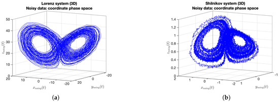
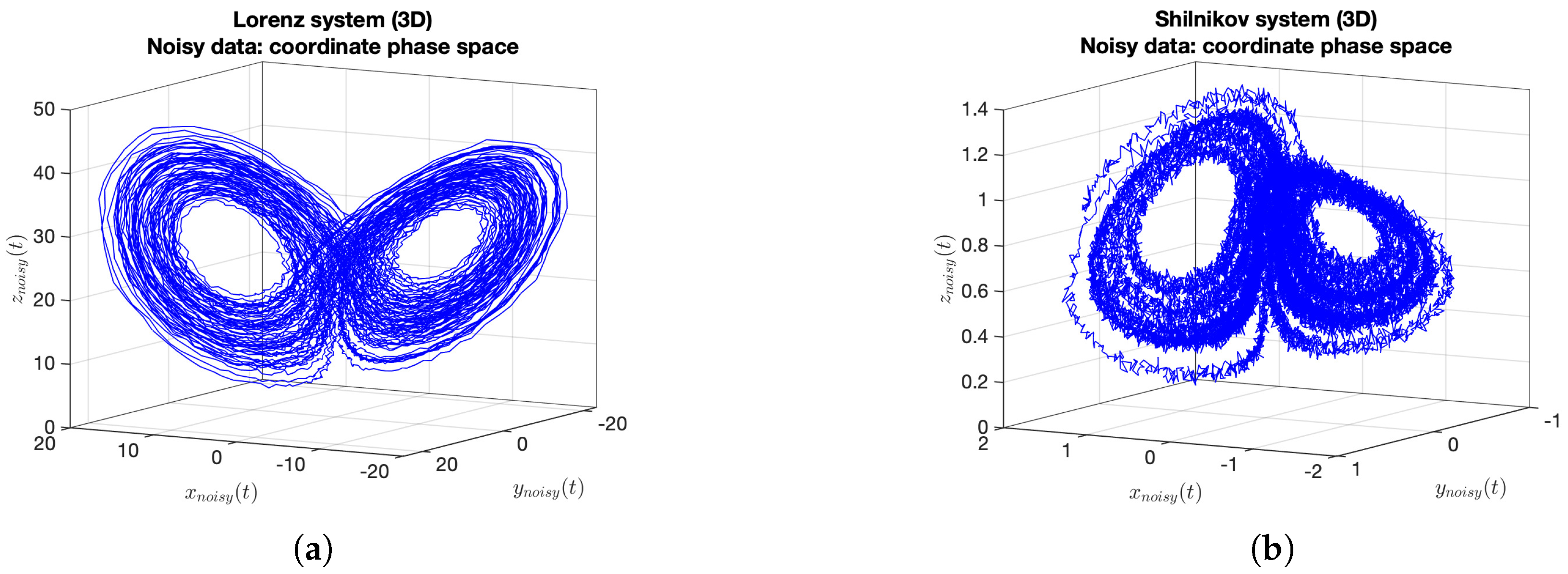
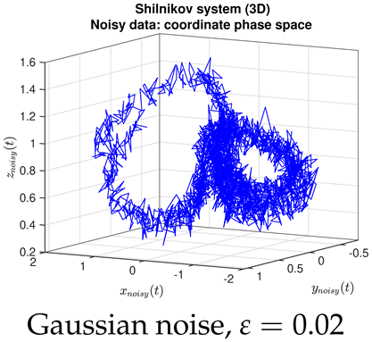
which is chaotic for $[\alpha ,\lambda ,B]=\left[{\displaystyle \frac{4\sqrt{30}}{135}},{\displaystyle \frac{11\sqrt{30}}{90}},{\displaystyle \frac{2}{13}}\right]$. Phase plots of these systems with added Gaussian noise (see below) are shown in Figure 1a,b.

Figure 1. Calculated noisy data for added Guassian noise with $\mu =0$, $\sigma =1$, and $\epsilon =0.2$: (a) Lorenz system and (b) Shil’nikov system.

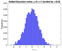
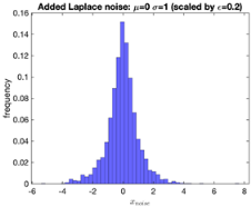
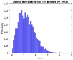
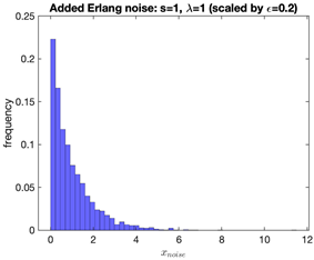
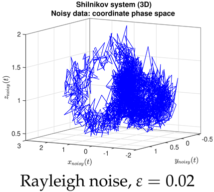
The analyses were conducted in Matlab 2021b on a MacBook Pro with 2.3 GHz Intel Core i9, with numerical integration by the ode45 function. For each system, the data $\mathit{X}$ were calculated and augmented by additive random noise using the function ${\mathit{X}}_{noisy}=\mathit{X}+\epsilon {\mathit{X}}_{distrib}$, where ${\mathit{X}}_{distrib}$ is sampled from a univariate noise distribution and $\epsilon$ is a scaling parameter. Four noise models with random variable y were considered, illustrated in Table 1. These include two symmetric noise models (Gaussian and Laplace with $\mu =0$) and two non-negative skewed noise models (Rayleigh and Erlang). Only the Gaussian noise model conforms to the assumption of Gaussian error (10), so the other models provide a test of robustness of the algorithms used. The noisy derivatives ${\dot{\mathit{X}}}_{noisy}$ were then calculated from the noisy data ${\mathit{X}}_{noisy}$ by a dynamical system function call.

Table 1. Noise models adopted in this study.

Gaussian noise	Laplace noise	Rayleigh noise	Erlang noise
$\eta ={\displaystyle \frac{1}{\sigma \sqrt{2\pi }}}exp\left(-{\displaystyle \frac{{(y-\mu )}^2}{2{\sigma }^2}}\right)$	$\eta ={\displaystyle \frac{1}{\sigma \sqrt{2}}}exp\left(-{\displaystyle \frac{\sqrt{2}|y-\mu |}{\sigma }}\right)$	$\eta ={\displaystyle \frac{y}{{\sigma }^2}}exp\left(-{\displaystyle \frac{y^2}{2{\sigma }^2}}\right)$	$\eta ={\displaystyle \frac{{\lambda }^s{y}^{s-1}{e}^{-\lambda y}}{(s-1)!}}$
		for $y\ge 0$	for $y\ge 0$
mean $\mu$, standard deviation $\sigma$	mean $\mu$, scale $\sigma /\sqrt{2}$	scale $\sigma$	shape s, rate $\lambda$

The data were then analyzed by three traditional regularization algorithms (SINDy, LASSO, ridge regression) and two Bayesian algorithms (JMAP and VBA), using inbuilt Matlab functions for LASSO and ridge regression, and modified forms of published codes for SINDy [2], JMAP, and VBA [6]. All analyses were conducted using an inner iteration for fixed hyperparameter(s), and an outer iteration over a sequence of hyperparameter(s). For SINDy, iteration was conducted over $\lambda$, proceeding from a high value, while for LASSO and ridge regression, iteration was conducted over each ${\kappa }_j$. For JMAP and VBA, a broad Gaussian model prior and covariance prior with fixed hyperparameters $\{{\alpha }_{{\Xi }_{\ell j}},{\beta }_{{\Xi }_{\ell j}}\}$ were selected, to represent the a priori belief that the model coefficients should be symmetric about zero, penalising coefficients approaching $\pm \infty$. The outer iteration was then conducted over the error hyperparameters $\{{\alpha }_{{ϵ}_{ij}},{\beta }_{{ϵ}_{ij}}\}$, combined into the inverse gamma expectation ${\beta }_{{ϵ}_{ij}}/({\alpha }_{{ϵ}_{ij}}-1)$. In each method, the 2-norms and (where available) Gaussian norms were examined.

4. Results

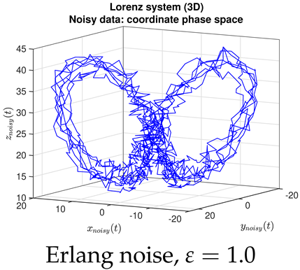
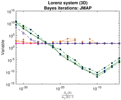
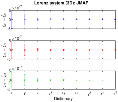
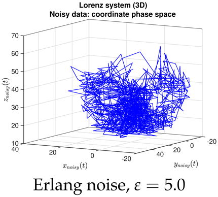
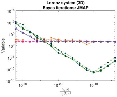
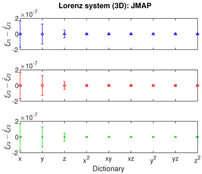
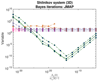
The outputs from several sets of analyses are shown below, including for the Lorenz system with Gaussian noise analyzed by different methods (Table 2), and the Lorenz or Shil’nikov systems with different noise models analyzed by JMAP (respectively, Table 3 and Table 4). From these and other analyses, we can interpret the following:

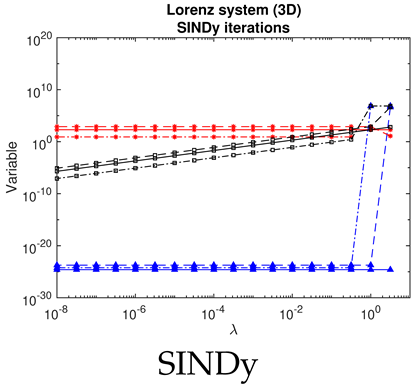
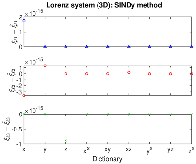
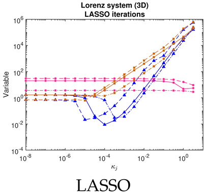
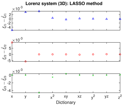
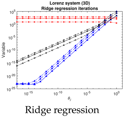
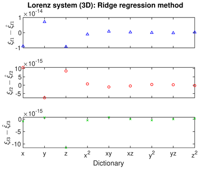
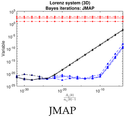
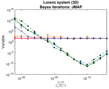
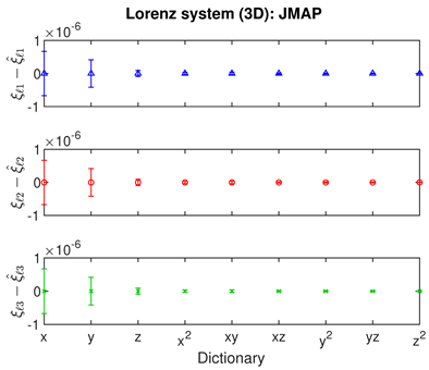
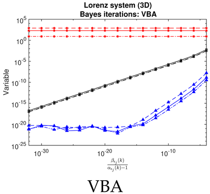
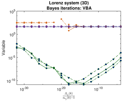
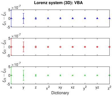
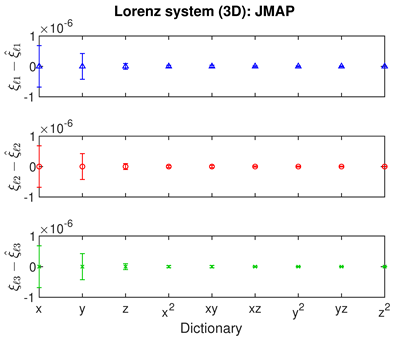
Table 2. Analyses of the Lorenz system ($t=10$, $t_{step}=0.01$) with Gaussian noise ($\mu =0,\sigma =1,\epsilon =0.2$) by SINDy, LASSO, ridge regression, JMAP, and VBA, showing (column 1) plots of residual, regularization term and the objective function; (column 2) plots of prior, likelihood, and posterior Gaussian norms (where available); and (column 3) differences in predicted parameters ${\xi }_{ij}-{\widehat{\xi }}_{ij}$, with predicted standard deviations shown as error bars for JMAP and VBA.

2-Norm Plots	Gaussian Norm Plots	Coefficient Plots
	Not applicable
	Not applicable

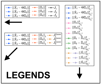
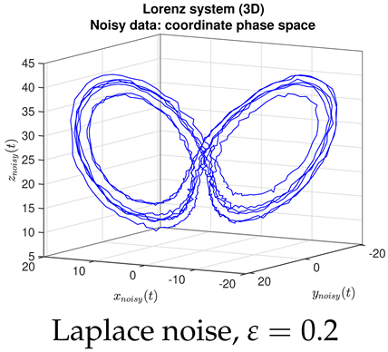
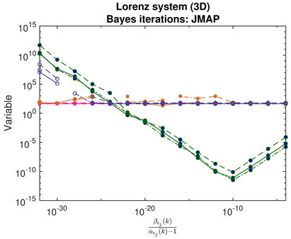
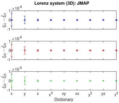
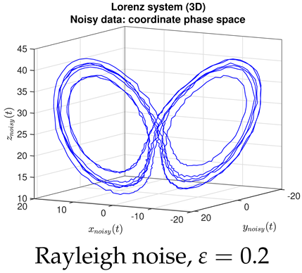
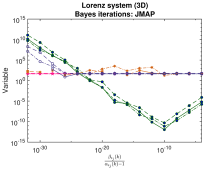
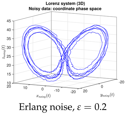
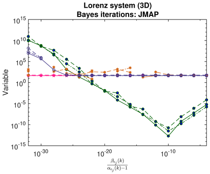
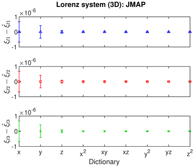
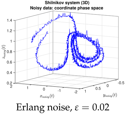
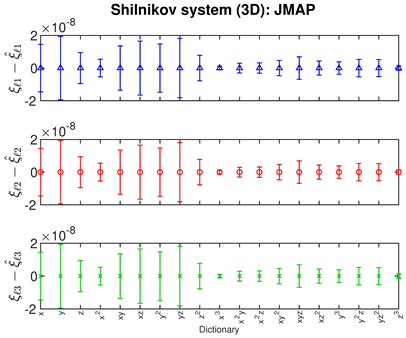
Table 3. Analyses of the Lorenz system ($t=10$, $t_{step}=0.01$) by JMAP for various noise models ($\mu =0,\sigma =s=\lambda =1$) of different scales $\epsilon$, showing (column 1) the phase plot of noisy data; (column 2) plots of prior, likelihood, and posterior Gaussian norms; and (column 3) differences in predicted parameters ${\xi }_{ij}-{\widehat{\xi }}_{ij}$, with predicted standard deviations shown as error bars. The legend for column 2 is for Table 2.

Phase Plots	Gaussian Norm Plots	Coefficient Plots

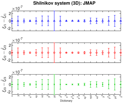
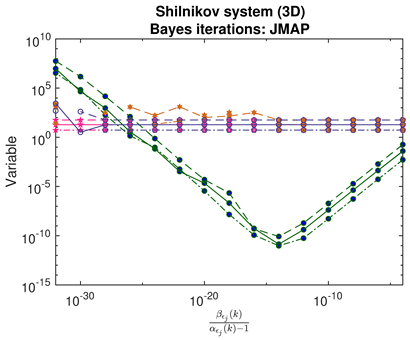
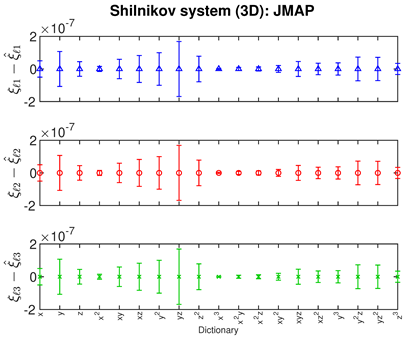
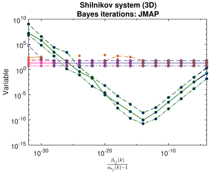
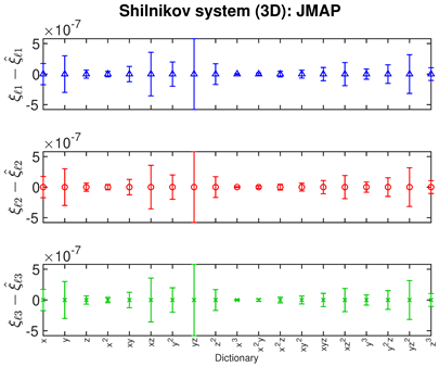
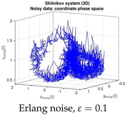
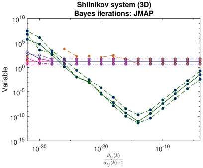
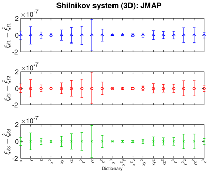
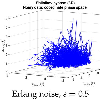
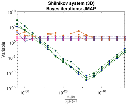
Table 4. Analyses of the Shil’nikov system ($t=50$, $t_{step}=0.02$) by JMAP for various noise models ($\mu =0,\sigma =s=\lambda =1$) of different scales $\epsilon$, showing (column 1) the phase plot of noisy data; (column 2) plots of prior, likelihood, and posterior Gaussian norms; and (column 3) differences in predicted parameters ${\xi }_{ij}-{\widehat{\xi }}_{ij}$, with predicted standard deviations shown as error bars. The legend for column 2 is for Table 2.

Phase Plots	Gaussian Norm Plots	Coefficient Plots

• For JMAP and VBA, the optimum in $\{{\alpha }_{{ϵ}_{ij}},{\beta }_{{ϵ}_{ij}}\}$ is identified by a minimum in the posterior Gaussian norm $\left|\right|{\Xi }_j-{\widehat{\Xi }}_j{\left|\right|}_{{{\widehat{\Delta }}_j}^{-1}}^2$ (green curves, column 1 of Table 2; column 2 of Table 3 and Table 4). This optimum corresponds to the maximum in the posterior (14), and is distinct in all examples considered. Both algorithms are fairly efficient in finding the optimum (∼5–10 iterations).
• For SINDy and ridge regression, the optimum in the threshold $\lambda$ or regularization parameter ${\kappa }_j$ is identified by a turning point in the residual $\left|\right|{\dot{\mathit{X}}}_j-\Theta {\Xi }_j{\left|\right|}_2^2$ (blue curves, column 1 of Table 2). In contrast, for LASSO, the residuals follow strange curves; the optimum is instead identified by a turning point in the objective function (brown curves, column 1 of Table 2). The SINDy method is very efficient (∼4–5 iterations) in finding the optimum, while LASSO and ridge regression require many more iterations.
• The Bayesian methods provide standard deviations on the predicted coefficients, extracted from the posterior covariance ${\widehat{\Delta }}_j$ in (14) (error bars, column 3 of Table 2, Table 3 and Table 4). These are of order ∼${10}^{-8}$–${10}^{-6}$ in all examples. In contrast, SINDy and ridge regression report a coefficient precision of ∼${10}^{-15}$–${10}^{-14}$. The inconsistency with JMAP and VBA suggest that this high precision is artificial. LASSO was unsuccessful in all examples examined, with a precision of ∼${10}^{-3}$ and poor recovery of the dynamical system.
• Contrary to our expectations, JMAP and VBA based on Gaussian noise (13) were highly robust to different choices of additive noise, for all dynamical systems, noise models, and parameter choices examined. Little difference was observed between the symmetric or non-negative noise models, even for such high magnitudes of added noise $\epsilon$ that the dynamical system becomes overwhelmed by noise (column 1 of Table 2 and Table 3).

5. Conclusions

In this study, we consider the problem of system identification of a dynamical system, represented by a nonlinear equation system $\dot{\mathit{x}}=f\left(\mathit{x}\right)$, from discrete time-series or spatial data. We propose a Bayesian framework based on the maximum a posteriori (MAP) point estimate, to give a generalized form of Tikhonov regularization with the residual and regularization terms identified, respectively, with the negative logarithms of the likelihood and prior distributions. As well as estimates of the model coefficients, the Bayesian interpretation provides access to the full Bayesian apparatus, including the ranking of models, the quantification of model uncertainties, and the estimation of unknown (nuisance) hyperparameters. The present study employs two Bayesian algorithms for hyperparameter estimation, the joint maximum a posteriori (JMAP) and variational Bayesian approximation (VBA), which are compared to the popular SINDy, LASSO, and ridge regression algorithms. For multivariate Gaussian likelihood and prior distributions, the Bayesian formulation gives a Gaussian posterior distribution, in which the numerator contains a Mahalanobis distance or “Gaussian norm”. We consider two dynamical systems (Lorenz and Shil’nikov), with four choices of noise model (Gaussian, Laplace, Rayleigh, and Erlang). Both JMAP and VBA algorithms were successful for model identification and uncertainty quantification, with predicted standard deviations in the model coefficients of ∼${10}^{-8}$–${10}^{-6}$ in all examples. This compares to the calculated precision of ∼${10}^{-15}$–${10}^{-14}$ by SINDy and ridge regression, which we consider to be artificially low. LASSO was unsuccessful in all examples examined. For the Bayesian algorithms, the posterior Gaussian norm is found to provide a robust metric for quantitative model selection for all combinations of dynamical system and noise model examined.

References

- Brunton, S.L.; Proctor, J.L.; Kutz, J.N. Discovering governing equations from data by sparse identification of nonlinear dynamical systems. Proc. Natl. Acad. Sci. USA 2016, 113, 3932–3937. [Google Scholar] [CrossRef] [Scilit] [PubMed]
- Mangan, N.M.; Kutz, J.N.; Brunton, S.L.; Proctor, J.L. Model selection for dynamical systems via sparse regression and information criteria. Proc. R. Soc. Proc. A 2017, 473, 20170009. [Google Scholar] [CrossRef] [Scilit] [PubMed]
- Rudy, S.H.; Brunton, S.L.; Proctor, J.L.; Kutz, J.N. Data-driven discovery of partial differential equations. Sci. Adv. 2017, 3, e1602614. [Google Scholar] [CrossRef] [Scilit] [PubMed]
- Hoerl, A.E.; Kennard, R.W. Ridge regression: Biased estimation for nonorthogonal problems. Technometrics 1970, 12, 55–67. [Google Scholar] [CrossRef]
- Santosa, F.; Symes, W.W. Linear inversion of band-limited reflection seismograms. SIAM J. Sci. Stat. Comput. 1986, 7, 1307–1330. [Google Scholar] [CrossRef] [Scilit]
- Mohammad-Djafari, A. Inverse problems in signal and image processing and Bayesian inference framework: From basic to advanced Bayesian computation. In Proceedings of the Scube Seminar, L2S, CentraleSupelec, Gif-sur-Yvette, France, 27 March 2015. [Google Scholar]
- Tarantola, A. Inverse Problem Theory and Methods for Model Parameter Estimation; SIAM: Philadelphia, PA, USA, 2005. [Google Scholar]
- Mohammad-Djafari, A.; Dumitru, M. Bayesian sparse solutions to linear inverse problems with non-stationary noise with Student-t priors. Digit. Signal Proc. 2015, 47, 128–156. [Google Scholar] [CrossRef] [Scilit]
- Lorenz, E.N. Deterministic nonperiodic flow. J. Atmos. Sci. 1963, 20, 130–141. [Google Scholar] [CrossRef] [Scilit]
- Shil’nikov, A.L.; Shil’nikov, L.P.; Turaev, D.V. Normal forms and Lorenz attractors. Int. J. Bifurc. Chaos 1993, 3, 1123–1139. [Google Scholar] [CrossRef] [Scilit]
Disclaimer/Publisher’s Note: The statements, opinions and data contained in all publications are solely those of the individual author(s) and contributor(s) and not of MDPI and/or the editor(s). MDPI and/or the editor(s) disclaim responsibility for any injury to people or property resulting from any ideas, methods, instructions or products referred to in the content. |
© 2025 by the authors. Licensee MDPI, Basel, Switzerland. This article is an open access article distributed under the terms and conditions of the Creative Commons Attribution (CC BY) license (https://creativecommons.org/licenses/by/4.0/).