


Abstract
This paper solves the open problem mentioned by Lin that was published in 2026 of Algorithms to prove the uniqueness property for the solution procedure proposed by Lin. The developed mathematical verification fulfills the research gap left by Lin. Moreover, for the local maximum point near the starting point (denoted as ) of the amelioration inventory model, this study presents an alternative explanation to help researchers execute their numerical methods with confidence such that, without the analytical procedure developed by Lin, only a rough numerical method can help researchers locate two local maximum points.
1. Introduction
Hwang [1] was the original paper to examine inventory models with amelioration effect. He developed two inventory models, (i) the economic ordering quantity model and (ii) the partially selling quantity model, with ameliorated items such that the storage items will be self-reproduced. Lin [2] mentioned an example of fish being raised in a closed pond. Chou et al. [3] and Tuan et al. [4] studied and improved the economic ordering quantity model proposed by Hwang [1]. Lin [2] examined and revised the economic ordering quantity model developed by Hwang [1]. Lin [2] also checked those 163 papers cited by Hwang [1] in their references to claim that Lin [2] is the first paper to modify the partially selling quantity considered by Hwang [1].
Lin [2] provided a revised solution procedure for the partially selling quantity model of Hwang [1]; based on the same numerical example, the maximum profit value proposed by Hwang [1] is about of that derived by Lin [2], showing the significant improvement obtained by Lin [2]. However, in the discussion of limitations of his solution procedure, Lin [2] admitted that he only finished the existent property for the zeros for his auxiliary function, and then Lin [2] raised an open problem for proving the uniqueness property for his solution process. This study will fulfill the research gap to prove the uniqueness property to answer the open problem proposed by Lin [2].
Moreover, Lin [2] emphasized that as his second main contribution, “purely applying a numerical algorithm to search for the global maximum point is not reliable” to illustrate the usefulness of his mathematical method. This study will provide a novel theorem to prove the existence of a local maximum between (i) a local minimum point and (ii) a boundary point, where the objective function will decrease to negative infinity. Thus, without the sophisticated mathematical derivations proposed by Lin [2], even a rough numerical estimation guarantees the existence of a local maximum point near . Therefore, this paper not only provides a revision to fulfill the research gap in the theoretical development of Lin [2], but also presents an alternative approach, without the complicated analysis examination proposed by Lin [2], to point out the local maximum point very close to .
The main contribution of this paper is threefold. First, this paper fulfills the mathematical foundation for the partially selling quantity model, constructed by Hwang [1], and then further examined by Lin [2] to provide a uniqueness analysis for the solutions of , which addresses the open problem mentioned by Lin [2]. Second, this paper presents a novel theorem, without the complex solution procedure developed by Lin [2], so that researchers will still have confidence to execute numerical methods to search the local maximum point, denoted as . Third, the questionable derivation of Lemma 2 in Lin [2] is improved. Several related papers, including Adamu and Yakubu [5], Marchi et al. [6], Gwanda [7], and Adamu and Yakubu [8], were added to illustrate the current development of amelioration inventory models.
This paper is organized as follows. We briefly review those related papers in Section 1. We introduce notation and assumptions in Section 2. We provide a brief review for solution algorithms of Lin [2] in Section 3 such that we can present our improvements for the uniqueness problems in Section 4 and an alternative solution procedure to locate the maximum point near zero (denoted as ) in Section 5. This structure separates inherited results from our new contributions. In Section 6, the questionable derivation of Lemma 2 in Lin [2] is explained and then revised. We conclude our discussion in Section 7.
2. Notation and Assumptions
To be compatible with Hwang [1] and Lin [2], we use the same notation as theirs. The notation and assumptions of the partial selling quantity model of Hwang [1] and Lin [2] are listed in the following.
is related to the first derivation of the objective function. is related to the first derivation of . The purpose of and is to present a solvable solution algorithm.
, , and are related to the sign of to help us to solve .
denotes the average total profit per unit time that consists of selling revenue, ordering cost, holding cost and the ameliorating cost (₩/day), which is the objective function.
denotes an auxiliary function, with
denotes another auxiliary function to simplify the derivations and help us to locate the solution of , with
denotes another auxiliary function to simplify the derivations and help us to locate the solution of , with
denotes the amelioration cost (₩/kg).
denotes the holding cost (₩/kg/day).
denotes the ordering cost (₩).
denotes an auxiliary function, with
such that .
denotes a second auxiliary function, with
such that .
denotes the inventory level (kg).
denotes the selling price per item.
denotes the constant demand rate (kg/day).
denotes the extra quantity to be sold at , with .
denotes the parameter to denote the time of amelioration (day).
denotes the cycle time (day).
denotes the solution of , for .
denotes the solution of , for and , which are critical points for the objective function, , with and , with . Lin [2] proved that and are local maximum points, and is a local minimum point.
denotes the optimal solution (day). Lin [2] derived that .
We assume the following novel notation.
is an auxiliary function.
is another auxiliary function.
is the solution for .
is the unique of , for .
, , , and are four abbreviations such that .
Because the proposed proof (see Table 1) relies on several auxiliary functions introduced at different stages of the derivation, we agree that readers may find it difficult to track the relationships among these functions. To improve readability and notation consistency, we have added a summary table listing all auxiliary functions, their mathematical definitions, and their roles in the solution procedure. The above addition enables readers to quickly identify the purpose of each function and better understand the overall proof structure.
Table 1.
Summary of auxiliary functions.
3. Review of the Related Model
The Partially Selling Quantity (PSQ) model was developed by Hwang [1] and then further explained by Lin [2]. Interested researchers are encouraged to refer to Lin [2] for his detailed explanations.
Lin [2] examined the PSQ model to maximize the average total profit,
with
Lin [2] plugged Equation (2) into Equation (1) to obtain the objective function,
For the partial selling quantity model proposed by Hwang [1], satisfying the restriction with the extra quantity will be sold at . Hence, , for , under the construction of Hwang [1].
Based on the numerical example proposed by Hwang [1], , , , , , , , and such that Lin [2] obtained that . Hwang [1] claimed that and . Hence, Lin [2] derived that , which is greater than the maximum value proposed by Hwang [1] and then he solved to find .
Lin [2] claimed that if , the second term of Equation (1) becomes a negative value, and then Lin [2] derived that
such that Lin [2] derived his first lemma.
Lemma 1
(Lin [2]). The searching domain for the maximum point for the objective function, , is reduced from an infinite region, , to a finite region, . The maximum problem becomes solvable.
Based on Equation (3), Lin [2] obtained that
where is an auxiliary function to simplify the expression, with
Lin [2] tried to determine the sign of such that he constructed to simplify the solution process.
Based on Equation (6), Lin [2] derived that
where is a second auxiliary function to simplify the expression, with
since Lin [2] tried to decide the sign of such that Lin [2] considered another auxiliary function, , that has the same sign as .
Motivated by Equation (8), Lin [2] assumed the third auxiliary function, denoted as such that
which is a decreasing function. Lin [2] derived that the maximum value , and the minimum value , to support the assertion of , for .
To simplify the expression, Lin [2] defined that
and
such that
Lin [2] defined as the solution of to obtain that , and then he derived , such that if , then .
Lin [2] tried to solve , that is, to solve to imply that , and then if , then , and for , . Therefore, Lin [2] proved that , for .
Remark 1.
In Section 4, we will define a new notation, , in Equation (22), for our later discussion.
Lin [2] computed at to derive that , with , and
and then for Lin [2] showed that
to obtain that .
Lemma 2
(Lin [2]). , for , to shrink the searching region of , from to .
We will show that the assertion of Lemma 2 proposed by Lin [2] is valid, but his derivation as cited as Equation (14) contained questionable results, which will be improved in Section 6.
Lin [2] computed , , and , according to the Intermediate Value Theorem of a continuous function (Thomas and Finney [9]), to claim that has two solutions, denoted as and , with and .
Lemma 3
(Lin [2]). has two solutions, , and , with .
In Section 7 of Lin [2], entitled “The Limitations of Our Study”, he mentioned that based on the Intermediate Value Theorem of a continuous function, he claimed the existence of at , and , with . However, Lin [2] did not consider the uniqueness property, and then he raised an open question to prove that has a unique solution for and , respectively. His assertion motivates us to provide a patch to fulfill this research gap in Section 4.
Based on Lemma 3, Lin [2] derived that and , and then he obtained that , for , , for , and , for . Moreover, referring to Lemma 2, where , for , Lin [2] claimed that , for .
Remark 2.
Owing to Equation (6), Lin [2] implied that , for , , for , and , for . Hence, decreases for and , and increases for , such that he computed that , , , and .
decreases from to to imply that there is a unique solution for , denoted as . Similarly, increases from to to imply that there is a unique solution for , denoted as . At last, decreases from to to imply that there is a unique solution for , denoted as .
Based on our above discussion, for , there is no uniqueness problem for , in each sub-domain, , and .
Lin [2] derived that , , and . Later, he proved that and are two local maximum points and is a local minimum point in Lemmas 4 and 5, and Theorem 1 of Lin [2]. We agree with his derivations of Lemmas 4 and 5, and Theorem 1 of Lin [2].
Hence, to save the precious space of this journal, we will not review Lemmas 4 and 5 further, nor Theorem 1 of Lin [2]. Interested readers are encouraged to refer to Lin [2].
In Section 6 of Lin [2], entitled “Analytical Results to Support the Numerical Algorithm”, with Table 1 of Lin [2], he claimed that if researchers applied a numerical method to search extreme points for of Equation (3), then without the analytical results derived by Lin [2], it would be very difficult to find a local maximum point of . We will present an alternative approach in Section 5 to demonstrate that without the sophisticated mathematical development proposed by Lin [2], researchers still have motivation to find .
4. Uniqueness Problem for in Each Sub-Domain
We agree with the assertion of Lin [2] that has two solutions, denoted as and with and , with
and
However, we raise an open question. Lin [2] only provided the existence property for with sub-domain: and . However, Lin [2] did not provide a discussion for the uniqueness for zeros in and , respectively. The purpose of this section is to present a revision for the uniqueness property to complete the unresolved uniqueness argument for on the intervals and .
We admit that is a continuous function, from , and , and then there is a zero for . It is an existence problem that is based on the Intermediated Value Theorem of calculus for any continuous function (Thomas and Finney [9]). However, Lin [2] did not consider the uniqueness problem, that is, to prove that has only one solution for .
Similarly, we agree to the existence problem for , with the sub-domain, with , and , that there exist zeros for in . However, this uniqueness problem is another open problem for .
We will try to prove that there is a point, denoted as , which is the unique solution for , and then , for , and , for . Thus, increases for , and decreases for , to prepare for our goal to prove that has only one solution for and another solution for , respectively, since Lin [2] already proved that , for ; therefore, we do not need to worry about .
Remark 3.
Owing to a technical problem, we slightly change the uniqueness problem from the pair of two intervals: and to another pair of two intervals: and . Finally, we will apply our findings for and , to the original pair: and , proposed by Lin [2].
We derive that
We rewrite Equation (17) as follows:
To analyze in Equation (18), we assume two auxiliary functions, and , as follows:
and
Based on in Equation (19), and in Equation (20), we can rewrite Equation (18) as follows:
According to Equation (19), we solve for to derive a point, denoted as , with
such that , and then for , we derive that
Referring to Equation (20), we derive that
Owing to Equation (24), we show that , and then is a decreasing function. We compute that
and
We combine the findings of Equations (25) and (26) to show that , , and is a decreasing function. Hence, we obtain that there is a unique point, denoted as that satisfies , and then we obtain that , for , and , for .
To further simplify the expression, we assume that
and
such that
Based on Equations (23) and (28), we derive that for .
Recalling the assumption of Hwang [1] and further examination of Lin [2] after Equation (9), we know that . According to Equation (29), is a positive function, and , for , and , for , we derive that , for , and , for .
Owing to (i) , for , and (ii) , for , and (iii) , for , and , for , we cannot present further analytical results for the sign of . Therefore, in the above, we provide a numerical examination to consider the sign of .
Referring to the second column in Table 2, is a positive and increasing function, from to , for .
Table 2.
Numerical results of , , , and , for .
Based on the third column in Table 2, is a negative and increasing function, from to , for .
Owing to the fourth column in Table 2, is a decreasing function from , to , and then we derive that
is the solution for , because of the definition of , such that we know that and have the same zero such that we use the same expression for the zero of and , simultaneously.
Based on the fourth column in Table 2, when , , and if , . Thus, is dominated by for and . Hence, we provide a finer and finer partition for , to obtain that ; ; ; ; and then we stop at and .
The fifth column in Table 2 reveals that is gradually decreasing from to such that has a unique solution, denoted as , with
which is the solution of , and then , for , and , for , such that increases for , and decreases for .
We confess that the sign of (that is, ) is not fully determined by this study for .
On the other hand, we study for to avoid the above dilemma of , with .
We recall of Equation (11) and of Equation (10), for , to imply that (i) , (ii) , (iii) , and (iv) , where and , since is an increasing function, is a decreasing function, is an increasing function, and is a decreasing function.
Hence, we recall of Equation (12), with , to assume a lower bound, denoted as LB, and an upper bound, denoted as UB, with
and
such that , for .
Based on the results of Equations (34) and (35), we can claim that
for , which is far away from zero.
We summarize our findings in the next theorem.
Theorem 1.
We prove that:
(i) For , increases from to such that has a unique solution, denoted as (defined by Lin [2]).
(ii) For , decreases from to such that has a unique solution, denoted as (defined by Lin [2]).
(iii) For , , which is far from zero such that has no solutions for .
Based on our Theorem 1, we derive the following finding.
Corollary 1.
We derive that
(1) For , has a unique solution, denoted as (defined by Lin [2]).
(2) For , has a unique solution, denoted as (defined by Lin [2]).
Based on our Theorem 1 and , derived by Lin [2], we know that for such that we can change the partition of from the previous partition: and to a new partition: and [1, 67.5]. Hence, we derive an improvement for Lemma 3 of Lin [2] as follows.
Corollary 2.
(1) For , has a unique solution, denoted as (defined by Lin [2]).
(2) For , has a unique solution, denoted as (defined by Lin [2]).
Therefore, we provide an improvement for the uniqueness property for in and , respectively, with respect to Lemma 3 in Lin [2].
5. An Alternative Proof for the Local Maximum Point
This section offers a complementary explanation for why a refined numerical search near is warranted once the boundary behavior and the interior local minimum are taken into account.
Recall of Equation (15), and of Equation (16). Lin [2] computed , , , and , and then Lin found that has three solutions, denoted as ,, and such that , , and , with the following Table 3, which is a reproduction of Table 1 in Lin [2], finding that
and
Table 3.
Reproduction of Table 1 of [2]. Numerical algorithm to compute ATP values.
Lin [2] asserted this based on his solution procedure with and , such that has a solution for , and then researchers can have confidence in executing the following numerical operation to search for , which is a reproduction of Table 1 of Lin [2].
In Lemma 5 of Lin [2], he proved that and are two local maximum points, and is a local minimum point.
On the other hand, Lin [2] claimed that if a practitioner only used a numerical method to search for the local extreme value for the objective function, , with partition size , then they will derive the following Table 4.
Table 4.
Numerical results for , with partition size 1.
Table 4 is an estimation of , where is restricted to natural numbers to provide a bird’s-eye view for the figure of .
Based on Table 4, practitioners found that (i) is a local minimum point, and (ii) is a local maximum point, for integer solutions.
The above observation is consistent with the real number solution of of Equation (38), which is a local minimum point, and of Equation (39), which is a local maximum point.
If the practitioner tries to search the critical point for , because is not defined, he will test to derive the third row of Table 3 to imply that is a decreasing function for .
For a finer partition, the practitioner will test to derive the second row of Table 3 to imply that is a decreasing function for , as the fourth row of Table 3.
Repeating this process, to shrink the partition size to (a) , (b) 0.0001, and (c) 0.00001, he will then imply that is a decreasing function for (a) , (b) , and (c) , as indicated in the fifth, sixth, and seventh rows of Table 3.
Usually, because the partition size is a very small number, the practitioner will stop his numerical test and conclude that there are no critical points for .
On the other hand, based on his analytical derivation, Lin [2] knew that there is a point, denoted as , with , which is a local maximum point. Hence, Lin [2] has confidence in executing his numerical computation, as in Table 3.
We disagree with the above assertion of Lin [2], that is, without those analytical results derived by Lin [2], only with the numerical findings of Table 4, and present an alternative approach to help researchers locate a critical point for .
We begin by evaluating the value of to compute that
We evaluate that
and by the Hospital rule,
to determine that , because and is a finite value, such that we derive that
For completeness, we apply a numerical algorithm to estimate , when . To simplify the expressions, we assume that
and
such that
We list the results in the following Table 5, to indicate that when , the value of the objective function, will go to negative infinity.
Table 5.
Numerical results for , when .
Based on Table 5, we realize that is relatively stable, approaching , when . increases to , by the effect of , and increases to , by the effect of , as the variable goes to zero. Thus, we imply .
Recalling Table 4, we know that , , and , to imply that there is a local minimum point around , such that we assume this local minimum point as .
We will use (i) , and (ii) as a local minimum point to verify that there exist local maximum points in .
More generally, we will abstractly derive the following results, under three conditions: (a) , (b) is a local minimum point, (c) . Then we will prove that there exist local maximum points in .
Given a value, denoted as , owing to , we can select a point, denoted as , with , to find an interval, denoted as , such that
for .
We will claim that
By way of contradiction, we assume that
We assume a positive number, denoted as , such that is defined as follows:
is a continuous function, for and , we can find an interval around , denoted as , satisfying , such that
We expand Equation (52) to obtain that
We plug Equation (51) into the first inequality of Equation (53) to derive that
We simplify the expression of Equation (54) to show that for ,
We apply Equation (50) to Equation (55), and then for , we obtain that
For those , Equation (56) implies that .
However, on the other hand, Equation (48) derives that , for .
Under the restriction of , for those , Equation (56) derives that . On the other hand, Equation (48) obtains that .
It is a contradiction such that the assumption of Equation (50) is false. Therefore, we finish the proof of Equation (49).
For the compact sub-domain , the continuous function will attain its maximum value. Without loss of generality, we assume that
We recall that is a local minimum point such that
Referring to Equation (49), it shows that
such that we obtain that
According to Equations (58) and (60), we know that must be an interior point, that is, such that
We find a local maximum point, , that satisfies . We summarize our results in the next theorem.
Theorem 2.
Under three conditions, (a) , (b) is a local minimum point, and (c) , we prove that there exist local maximum points in .
Based on above discussion, we claim that Hwang [1] and Lin [2] did not pay attention to . Moreover, Lin [2] was not familiar with Theorem 2 such that Lin [2] claimed that researchers applied numerical algorithms to search for and then generally they will stop their searching before reaching .
If researchers knew Theorem 2, then they would believe that there must be a local maximum point in . Consequently, our Theorem 2 will help practitioners take a finer grid to execute their numerical algorithms.
In Table 1 of Lin [2], he provided detailed data on how to find the local maximum point, . Interested readers are encouraged to refer to Table 1 of Lin [2].
We believe that our Theorem 2 will benefit researchers in the future to search for optimal solutions.
6. The Revision of Lemma 2 in Lin [2]
Lin [2] derived that if , then , which did not support his derivation of the following:
for in Equation (14).
To derive the inequality of Equation (62), a natural way for ordinary researchers is to prove that is a decreasing function for . Hence, we begin to compute to imply that
Owing to , this was claimed by Hwang [1] and further checked by Lin [2] as Equation (9) to imply the first term of Equation (63) is negative.
To prove , for the best approach is to check that
because of , for .
We compute that for
Based on Equation (65), we verify that the inequality on Equation (64) is valid, and then , is patched by us, and then the assertion of Equation (62) is proved by our improvement.
We accept that
in Equation (14), because recalling the definition of in Equation (11), it is trivial that is an increasing function.
For completeness, we point out that was mentioned in Lin [2], listed as Equation (13) in this paper. However, we compute that
and
such that the result of of Equation (13) proposed by Lin [2] is right. However, according to Equation (14), Lin [2] wanted
such that Lin [2] should use
Therefore, the result of in Lin [2] should be revised to .
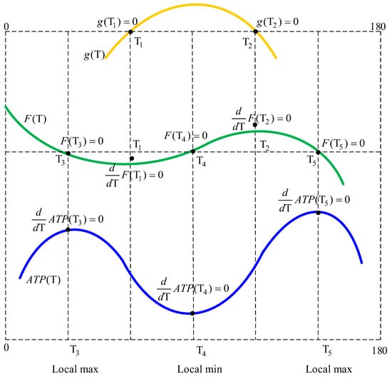
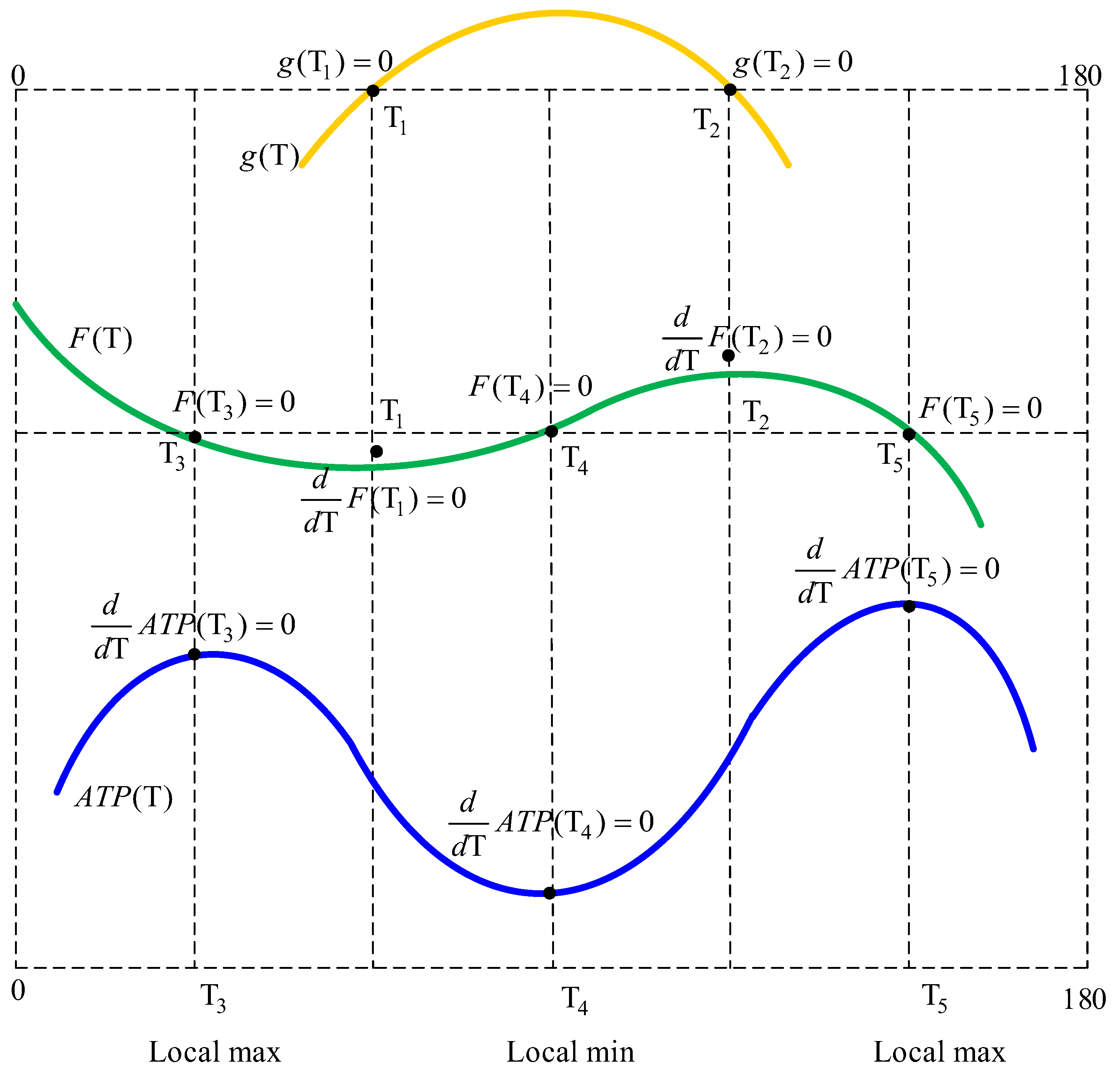
To provide a graphical representation for this study, we improve Figure 1 of Lin [2] as Figure 1 of this paper in the following such that the relationship between (a) the local extreme points and (b) the first derivation reaches zero, becoming visible.
Figure 1.
The upper picture: G(T) marked by yellow. The middle picture: F(T) marked by green. The lower picture: ATP(T) marked by blue. Reproduction of Figure 1 of Lin [2] with revisions.
7. Conclusions
This paper discusses how the proposed uniqueness results can assist practitioners by (1) reducing uncertainty in numerical optimization procedures, (2) narrowing the search region for candidate solutions, (3) improving computational efficiency, (4) increasing confidence in numerical implementations, and (5) providing a more reliable framework for solving amelioration inventory models. These practical implications help bridge the gap between mathematical theory and inventory management applications.
This paper solved the open question proposed by Lin [2] for the uniqueness property for the solutions of for and , respectively, to improve the quality of Lemma 3 of Lin [2]. The practical significance is improving confidence in numerical optimization procedures for amelioration inventory models. Based on our theoretical proof, researchers believe that the uniqueness property for in Lemma 3 of Lin [2] is verified and summarized in Theorem 1.
We also derived a novel theorem to prove that if the boundary value is negative infinity, then there must exist local maximum points between (i) the boundary and (ii) the local minimum point. Thus, the assertion of Lin [2] for the numerical examination is invalid. Our generalized result of Theorem 2 will help practitioners deal with related inventory models for local extreme points near the vertically infinite value problems.
We also provide an improvement for , owing to Lin [2], who already derived the monotonic property of , such that to solve , there is no uniqueness problem. Last but not least, we improved the proof for Lemma 2.
The limitations of the present study include the reliance on numerical verification for certain parts of the analysis and the possibility of extending the approach to broader inventory models in future research.
Based on the above discussion, this paper revised Lin [2] to provide a revised version for the amelioration inventory model proposed by Hwang [1].
Author Contributions
Conceptualization, Y.-N.C. and K.-C.H.; methodology, Y.-N.C.; software, C.-W.Y.; validation, Y.-N.C. and K.-C.H.; formal analysis, Y.-N.C.; investigation, Y.-N.C. and C.-W.Y.; resources, C.-W.Y.; data curation, C.-W.Y.; writing—original draft preparation, Y.-N.C.; writing—review and editing, K.-C.H.; visualization, C.-W.Y. and K.-C.H.; supervision, Y.-N.C.; project administration, Y.-N.C.; funding acquisition, K.-C.H. All authors have read and agreed to the published version of the manuscript.
Funding
This research received no external funding.
Data Availability Statement
The original contributions presented in this study are included in Lin [2]. Further inquiries can be directed to the corresponding author.
Conflicts of Interest
The authors declare no conflicts of interest.
References
- Hwang, H.S. A study on an inventory model for items with Weibull ameliorating. Comput. Ind. Eng. 1997, 33, 701–704. [Google Scholar] [CrossRef] [Scilit]
- Lin, S.S.C. Mathematical approach for ameliorated inventory models. Algorithms 2026, 19, 90. [Google Scholar] [CrossRef] [Scilit]
- Chou, S.; Chouhuang, W.T.; Lin, J.S.; Chu, P. An analytic solution approach for the economic order quantity model with Weibull ameliorating items. Math. Comput. Model. 2008, 48, 1868–1874. [Google Scholar] [CrossRef] [Scilit]
- Tuan, H.W.; Lin, S.C.; Julian, P. Improvement for amelioration inventory model with Weibull distribution. Math. Probl. Eng. 2017, 2017, 8946547. [Google Scholar] [CrossRef] [Scilit]
- Adamu, H.; Yakubu, M.I. A discrete time economic order quantity model for ameliorating items with constant demand. Trans. Niger. Assoc. Math. Phys. 2023, 19, 257–266. [Google Scholar]
- Marchi, B.; Zavanella, L.E.; Zanoni, S. Supply chain finance for ameliorating and deteriorating products: A systematic literature review. J. Bus. Econ. 2023, 93, 359–388. [Google Scholar]
- Gwanda, Y.I. Economic Order Quantity (EOQ) Model: Weibull ameliorating items with constant demand rate. FUDMA J. Sci. 2024, 8, 344–349. [Google Scholar] [CrossRef] [Scilit]
- Adamu, H.; Yakubu, M.I. A discrete time economic order quantity model for ameliorating items with constant holding cost and linear demand. J. Basics Appl. Sci. Res. 2025, 3, 111–125. [Google Scholar] [CrossRef] [Scilit]
- Thomas, G.B.; Finney, R.L. Calculus with Analytic Geometry, 9th ed.; Addison-Wesley Publishing Company: Reading, MA, USA, 1996; pp. 92–93. [Google Scholar]

Disclaimer/Publisher’s Note: The statements, opinions and data contained in all publications are solely those of the individual author(s) and contributor(s) and not of MDPI and/or the editor(s). MDPI and/or the editor(s) disclaim responsibility for any injury to people or property resulting from any ideas, methods, instructions or products referred to in the content. |
© 2026 by the authors. Licensee MDPI, Basel, Switzerland. This article is an open access article distributed under the terms and conditions of the Creative Commons Attribution (CC BY) license.