Enhanced Assumption-Aware Linear Discriminant Analysis for the Wisconsin Breast Cancer Dataset: A Guide to Dimensionality Reduction and Prediction with Performance Comparable to Machine Learning Methods

Abstract

The analysis of multivariate data is a central issue in biomedical research, where the accurate classification of patients and the extraction of reliable conclusions are of critical importance. Linear Discriminant Analysis (LDA) remains one of the most established methods for both dimensionality reduction and classification of data. In this paper, we examine in detail the theoretical foundations, assumptions, and statistical properties of LDA, and apply the method step by step to real data from the Breast Cancer Wisconsin (Diagnostic) database, which includes cellular features from breast biopsy samples with the aim of distinguishing benign from malignant tumors. Emphasis is placed on the importance of the method’s assumptions, such as multivariate normality, equality of covariance matrices, and absence of multicollinearity, demonstrating that their fulfillment leads to significant improvements in model performance. Specifically, careful preprocessing and strict adherence to these assumptions increase classification accuracy from $95.6\%$ ($94.7\%$ cross-validated) to $97.8\%$ ($97.4\%$ cross-validated). To our knowledge, this study is the first to demonstrate the dual use of LDA as both a dimensionality-reduction tool and a predictive classification model for this medical database within the same biomedical analysis framework. Moreover, we provide, for the first time, a systematic comparison between our assumption-aware LDA model and related studies employing the most accurate machine-learning classifiers reported in the literature for this dataset, showing that classical LDA achieves accuracy comparable to these more complex methods. The resulting discriminant model, which uses 13 variables out of the original 30, can be applied easily by clinical researchers to classify new cases as benign or malignant, while simultaneously providing interpretable coefficients that reveal the underlying relationships among variables. The implementation is carried out in the SPSS environment, following the theoretical steps described in the paper, thus offering a user-friendly and reproducible framework for reliable application. In addition, the study establishes a structured and transparent workflow for the proper application of LDA in biomedical research by explicitly linking assumption verification, preprocessing, dimensionality reduction, and classification.

1. Introduction

In many problems of medical research, as well as in everyday activities, the complexity of the phenomena under study and the widespread use of modern technology necessitate the simultaneous processing of large volumes of multivariate data. In Statistics and Machine Learning, a variety of methods have been developed for analyzing such data, depending on whether class labels are available. Supervised approaches, which rely on labeled data to build predictive models, include Multiple Linear Regression for modeling linear relationships with continuous outcomes [1,2], Logistic Regression for modeling class membership probabilities in binary response settings [3], and Linear Discriminant Analysis (LDA) for classification into known groups through linear combinations of explanatory variables that enhance group separability [4,5]. In addition, widely used machine learning algorithms include Support Vector Machines (SVM), which determine optimal separating hyperplanes with maximum margin [6], Random Forests and Decision Trees, which construct flexible, nonparametric decision rules via recursive partitioning and ensemble learning [7,8], and k-Nearest Neighbors (k-NN), which assigns class labels based on proximity in the feature space [9]. By contrast, unsupervised approaches are designed to uncover latent structure in the data without prior class labels and include clustering methods such as k-means, which partitions observations by minimizing within-cluster variance [10], and hierarchical clustering, which builds nested groupings based on pairwise similarity measures [11].

A third important category is formed by dimensionality reduction techniques, which aim to represent multivariate data in fewer dimensions while retaining the most relevant information. These methods can be unsupervised, such as Principal Component Analysis (PCA), which projects the data onto orthogonal directions of maximal variance [12,13], and Factor Analysis (FA), which explains observed correlations through a smaller number of latent factors [14,15], or supervised, such as LDA, which simultaneously reduces dimensionality and constructs a classification rule. Within this landscape, an especially important method for classifying multivariate data into existing groups, while at the same time reducing dimensionality, is Linear Discriminant Analysis.

Linear Discriminant Analysis constitutes a family of statistical methods for transforming an initial set of observations belonging to known groups with the dual aim of (i) interpreting the differences between these groups and (ii) classifying the observations as accurately as possible into the existing categories using selected discriminant variables. From a statistical perspective, LDA addresses the problem of assigning observations to the categories of a categorical, typically nominal, response variable on the basis of continuous independent variables measured on interval or ratio scales [16]. From a mathematical perspective, given a set of points in a multidimensional space, LDA constructs a lower-dimensional space spanned by a minimal number of new directions, referred to as discriminant functions, such that the projection of the original data facilitates group separation. This construction is obtained by solving a generalized eigenvalue problem involving the between-class and within-class covariance operators.

Its creator is Fisher (1936) [4], who used it to predict the national origin of individuals based on measurements on their skeleton. Applications of LDA exist in (a) Medicine: Disease diagnosis based on (i) certain symptoms, (ii) medical test results [17,18,19]; (b) Economics: Studying socio-economic differences between regions of a country [20]; (c) Archeology: Determining the sex of a human skeleton from measurements of the skull [21,22]; (d) Political Economy: Classification into parties of undecided individuals [23], etc.

Several recent works have sought to clarify LDA’s theoretical underpinnings and practical implementation. Tharwat et al. [24] presented a comprehensive tutorial on LDA, providing detailed mathematical derivations, visualizations, and numerical examples that build intuition and highlight common issues such as the small-sample-size problem and linear separability. In contrast, Qu and Pei [25] published a broad review focusing on recent methodological developments in LDA, including robust and kernel-based variants, adaptations for high-dimensional data, and strategies for handling multimodal distributions. While both contributions are valuable, they differ in scope: the former strengthens fundamental understanding, while the latter surveys modern methodological innovations. By contrast, the present work remains firmly within the framework of classical LDA, but distinguishes itself by offering a rigorous, assumption-driven application guide tailored to biomedical data, implemented step by step in Statistical Package for the Social Sciences (SPSS) for accessibility to clinical researchers. Moreover, the transparent structure and interpretable outputs of LDA make it particularly suitable for integration into decision–support and knowledge-based systems [26] for medical classification, while related data-driven frameworks addressing interpretability have been explored in oncological applications [27]. Recent developments in applied statistics continue to underline the versatility of classical LDA across a broad range of modeling scenarios. Notable methodological developments include functional LDA for high-dimensional curve data [28] and multiblock extensions for structured predictor sets [29], among several others. These extensions, while methodologically valuable, fall outside the scope of the present work, which focuses exclusively on classical LDA.

The present work contributes to this literature by offering a rigorous, step-by-step application of classical LDA to the Wisconsin Breast Cancer Diagnostic dataset. Our approach is distinctive in several respects:

• A theoretical foundation: We provide a complete guide to LDA, with a detailed account of its theoretical basis, assumptions, and statistical properties, including conditions of multivariate normality, equality of covariance matrices, and the absence of multicollinearity, and we show how these assumptions can be tested and satisfied in practice.
• A practical guide: Following the theory, we present a transparent step-by-step application of LDA in SPSS, enabling clinical researchers to apply the method reliably to real-world biomedical data.
• Dual use of LDA: To our knowledge, this is the first study to demonstrate LDA as both a dimensionality reduction tool and a classification model within the same biomedical framework.
• Improved predictive accuracy: We demonstrate how carefully satisfying the assumptions of LDA leads to measurable improvements in prediction, thereby emphasizing the critical importance of diagnostic checks prior to model use.
• Comparison with machine learning methods: Finally, we show that LDA, despite its conceptual simplicity and interpretability, can achieve classification accuracy comparable to more complex machine learning models while retaining the advantages of transparency and immediate applicability for the binary distinction between malignant and benign tumors.

2. Theoretical Framework of LDA

This section presents the purpose, objectives, and underlying assumptions of Linear Discriminant Analysis (LDA) in a detailed and rigorous manner. The implementation of Simple and Multiple Linear Discriminant Analysis is described. The discriminant functions (especially Fisher’s rule [4]), their number, characteristics, construction method, statistical tests for their significance, and their interpretation are described. In addition, methods for examining the significance of the (initial) variables are provided. Methods for classifying observations and evaluating the accuracy of such classifications are discussed. Any potential application problems of the method are described, and alternative forms of the method are presented (e.g., nonlinear D.A. [30,31]).

2.1. The Main Points of LDA

The purpose of Linear Discriminant Analysis can be summarized as follows:

(a)

Exploring the differences between (pre-existing) groups/classes;

(b)

Determining the most “economical” way of separating these groups;

(c)

Eliminating variables/characteristics that contribute minimally to group separation;

(d)

Testing the significance of each discriminant function;

(e)

Classifying new data/observations into the groups;

(f)

Evaluating the effectiveness of the classification rule constructed each time.

2.2. Comparison of LDA with Classification and Prediction Methods

LDA shares similarities and differences with other classification/prediction methods:

(a)

Cluster Analysis (C.A.)

In C.A., the data groups (and their number) are not known (in advance) and are created based on the similarities ("closeness") between observations (minimizing within-group dispersion) [16].

(b)

Logistic Regression (L.R.)

In L.R., the independent variables can be of any measurement type and are typically used when the dependent variable is binary. The coefficients in L.R. are easily interpretable, while in the discriminant functions only show the contribution of each variable to the discriminant function’s significance. L.R. calculates the probability of classifying an observation into a specific group and uses a cutoff rule to assign the observation to a particular group [3].

(c)

Multiple Linear Regression (M.L.R.)

Both methods can be considered prediction methods. M.L.R. is applied when the dependent variable is continuous (interval type) and provides predictions using a single function (regression line) involving weighted combinations of independent variables [32].

(d)

Analysis of Variance (ANOVA)

In one-way ANOVA, the independent variable is categorical, while the dependent variable is continuous (interval or ratio), whereas in LDA, the roles are reversed. In ANOVA, the focus is on the differences between groups in terms of their means, and it does not allow the classification of new observations [16].

(e)

Principal Component Analysis (P.C.A.)

Both methods aim to reduce the dimensionality of the data. P.C.A. does not consider group differences and cannot be used for classification. Additionally, the first principal component in P.C.A. captures the maximum variance in the data, and we use as many dimensions as deemed necessary [33].

2.3. Assumptions for Applying LDA

To apply LDA, the following assumptions should be met [16]:

(i)

The data can be classified into at least two known and mutually exclusive groups with similar sizes.

(ii)

The independent variables (features) used for group separation (discriminant variables) are measured on a scale of interval or ratio.

(iii)

Multicollinearity should be avoided. The independent variables should not be strongly correlated, as the predictive ability of the constructed model decreases with increasing correlation between these variables. In the case of strong correlations, an alternative analysis method such as logistic regression can be used (with fewer assumptions).

(iv)

The observations should constitute a random sample, with at least two observations per group. The sample size of the smallest group should, according to some authors, be larger than the number of independent variables (at least by two), while others suggest having a minimum of five cases for each independent variable.

(v)

The number of outliers should be minimized, or they have to be eliminated.

(vi)

Homoscedasticity should be ensured. The covariance matrices of the independent variables should be equal for each group. LDA is robust when this assumption is not satisfied and can be corrected through appropriate data transformations. The assumption can be examined using the Box-M test [5,16], which is sensitive to deviations from normality. An alternative way to test the assumption is to check the equality of determinants of the individual covariance matrices.

(vii)

Normality should be observed within each group, meaning that each group should follow a multivariate normal distribution with respect to the characteristics. LDA is robust when this assumption is not satisfied, if the non-normality is not due to the presence of outliers. An alternative approach to address non-normality is to transform the data (e.g., square root, inverse values, etc.).

2.4. Discriminant Functions

The idea behind constructing group-separating functions, called discriminant functions, is as follows: these functions (new axes) are obtained as linear combinations of the independent variables in a way that maximizes the distinctiveness between the specified groups. Thus, the first axis is chosen in such a way that the dispersion (variance) between the groups is maximized, while the dispersion within each group is minimized. It is the axis that optimally distinguishes the groups. Then, the second axis is chosen to be orthogonal to the first (uncorrelated new variables) and possesses the same property regarding variances [34].

The process continues until a (minimum) “suitable” number of separating functions is constructed. A (normal) separating function has the following form:

$$f_l\left(m\right)=u_0+u_1{X}_{1l}\left(m\right)+u_2{X}_{2l}\left(m\right)+\dots +u_p{X}_{pl}\left(m\right),l=1,2,\dots ,g,m=1,2,\dots ,n$$

(1)

where $f_l\left(m\right)$ is the value (score) of the observation m in the l group; $u_j$ are the coefficients of the function; and $X_{jl}\left(m\right)$ is the value of $X_j$ for the observation m in the l group.

Regarding the number g of separating functions, we have the following proposition.

Proposition 1

(Dimension of the LDA Discriminant Space [5,32]). In an LDA problem with k groups of the dependent variable, the maximum number g of discriminant functions is provided by

(i) 

$g\le k-1$, i.e., one less than the number of groups, when $n\ge p$;

(ii) 

$g\le p$, where p is the number of variables, when the sample size is smaller than the number of variables $(n<p)$.

Remark 1

(Two-Group Case). In the case of two groups, optimal separation is achieved using a single discriminant function, regardless of the dimensionality of the data. Consequently, the data can be projected onto a single straight line, yielding a reduction to the minimum possible dimensionality.

2.5. The Construction and Interpretation of Discriminant Functions

To construct discriminant functions, we need a measure of the degree of the existing differences between the groups. The matrix of means and variances of the values of the variables is not sufficient. Therefore, we consider the variance–covariance matrix $T={\left(t_{ij}\right)}_{i,j=1}^p$ of the following variables:

$$t_{ij}=\sum _{l=1}^k\sum _{m=1}^{n_l}\left(X_{ilm}-X_{i..}\right)\left(X_{jlm}-X_{j..}\right)$$

(2)

where $n_l$ denotes the size of group l and k is the number of groups. Moreover,

$$X_{i..}={\displaystyle \frac{1}{n}}\sum _{l=1}^k\sum _{m=1}^{n_l}{X}_{ilm}$$

(3)

denotes the overall sample mean of variable $X_i$ (with $n={\sum }_{l=1}^k{n}_l$). Throughout this section, dot notation is used exclusively for sample means, whereas population means are denoted by ${\mu }_k$. Using this matrix, we obtain a picture of how scattered the data points are in the space of variables (variance between the groups). The variance of the points within the groups can be measured using the within-groups covariance matrix $W={\left(w_{ij}\right)}_{i,j=1}^p$. Its elements are provided by

$$w_{ij}=\sum _{l=1}^k\sum _{m=1}^{n_l}\left(X_{ilm}-X_{il.}\right)\left(X_{jlm}-X_{jl.}\right)$$

(4)

where

$$X_{il.}={\displaystyle \frac{1}{n_l}}\sum _{m=1}^{n_l}{X}_{ilm}$$

(5)

denotes the corresponding sample mean of $X_i$ within group l [5].

When there are no differences between the centroids of the groups, the elements of the matrix W will be (almost) equal to the corresponding elements of the matrix T. However, if there are significant differences, the elements of W will be smaller than the elements of T. The difference between the two matrices is measured using the between-groups covariance matrix, denoted as $B=T-W$. By calculating these matrices and solving the generalized eigenvalue problem,

$$Bv=\lambda Wv,$$

(6)

we obtain the p eigenvalues $\lambda$ and the corresponding eigenvectors $v_{\lambda }={\left(v_i^{\left(\lambda \right)}\right)}_{i=1}^p$, which define the directions of the new axes.

Remark 2

(Standardized Discriminant Coefficients). The eigenvectors $v_{\lambda }$ obtained earlier serve as the coefficients for the separating functions. Therefore, by calculating the values (discriminant scores) of each observation with respect to these functions, we determine its location in the new space. However, because the raw coefficients lack direct interpretive meaning (and the associated scores are not inherently meaningful), the coefficients are typically standardized to produce the normalized coefficients u of the separating functions.

$$u_i=v_i\sqrt{n-k}\mathrm{and}{u}_0=-\sum _{i=1}^p{u}_i{X}_{i.}$$

The resulting scores can be used to assess the position of each observation in the new space. The discriminant scores are linear combinations of the original variables and are typically centered for interpretability; however, their variances depend on group dispersion and are not constrained to unity within each group. Thus, the score of an observation (with respect to a separating function) indicates its position on the axis defined by that function.

Normalization leaves the relative positions of the groups and their degree of separability unchanged. Its purpose is to shift the new axes so that they are centered on the overall centroid, making interpretation easier. In this normalized space, the location of any point can be assessed relative to the new coordinate system. Moreover, normalization removes the influence of the original measurement units, as distances are expressed in standard deviation units. Without this adjustment, classification would be biased toward groups with the largest dispersions. Consequently, a point’s distance reflects how many standard deviations it lies from the overall centroid.

The coefficients produced through this normalization procedure are referred to as unstandardized coefficients. If, however, the original data has already been standardized, then applying the same procedure yields the standardized coefficients. Discriminant scores are computed using the unstandardized coefficients. In this context, an unstandardized coefficient for a given separating function and variable indicates the change in an observation’s position along that separating function (axis) resulting from a one-unit increase in that variable, assuming all other variables remain constant [34].

2.6. Significance of Separating Variables

The contribution of a separating variable to the creation of a separating function can be estimated in two main ways [32,34]:

(I)

Standardized Coefficients: Although the unstandardized coefficients of the discriminant functions provide the absolute contribution of a separating variable in calculating a discriminant score, the information they provide can be “misleading” when a one-unit change in one measurement (variable) is not equivalent to a one-unit change in another (unequal/different units of measurement). To assess the relative importance of a variable, we consider the standardized coefficients $c_i=u_i\sqrt{{\displaystyle \frac{w_{ii}}{n-k}}}$. The magnitude of these coefficients helps us determine which variables contribute more to the calculation of discriminant scores.

(II)

Structure Coefficients/Discriminant Loadings: The similarity between a separating variable and a separating function is evaluated using their correlation coefficient. These correlations, known as structure coefficients or discriminant loadings, represent the cosine of the angle between the variable and the function in the data space, thus revealing the geometry of the space. A separating function is typically named according to the variables that show the strongest associations with it.

2.7. Number, Importance, and Significance of Separating Functions

The number of solutions in Equation (6) is equal to the number of (original) variables. Each solution (discriminant function) corresponds to an eigenvalue. However, it may happen that some of these solutions may be trivial ($\lambda =0$) and others may be statistically insignificant. The value of $\lambda$ is equal to the ratio $\lambda ={\displaystyle \frac{SSB}{SSW}}$ of the sum of squares between groups (SSB) to the sum of squares within groups (SSW) (from the corresponding analysis of variance with groups as a factor and the discriminant scores as the dependent variable). Therefore, the separating function associated with the largest $\lambda$ (SSB > SSW, indicating greater variance between groups) is the most important in terms of separability [32,34].

The importance of a discriminant function can be further examined using the following two methods: (I) dividing its corresponding eigenvalue ${\lambda }_i$ by the sum of all eigenvalues: ${\displaystyle \frac{{\lambda }_i}{{\sum }_j{\lambda }_j}}$. The quotient reveals the (relative) magnitude of the discriminant power of the separating function. For example, if ${\displaystyle \frac{{\lambda }_i}{{\sum }_j{\lambda }_j}}=0.847$, the first discriminant function contains $84.7\%$ of the total separability of the groups, meaning that it explains $84.7\%$ of the data variance. (II) Using the canonical correlation coefficient, which measures the relationship (correlation) between the groups and the discriminant function, given by the equation: $r_i^{*}=\sqrt{{\displaystyle \frac{{\lambda }_i}{1+{\lambda }_i}}}$. Instead of the term $r_i^{*}$, we typically use the term ${\eta }_{\iota }={\left(r_i^{*}\right)}^2={\displaystyle \frac{{\lambda }_i}{1+{\lambda }_i}}$ (coefficient of determination). The coefficient ${\eta }_{\iota }={\displaystyle \frac{{\lambda }_i}{1+{\lambda }_i}}={\displaystyle \frac{\frac{SSB}{SSW}}{1+\frac{SSB}{SSW}}}={\displaystyle \frac{SSB}{SSB+SSW}}={\displaystyle \frac{SSB}{SST}}$ (ratio of between-group sum of squares (SSB) to total sum of squares (SST)) indicates the proportion of variance in the scores (relative to the standard deviation) accounted for by the groups; thus, a higher value reflects a more important discriminant function.

The primary measure of a discriminant function’s statistical significance—known as the U statistic or Wilks’s lambda [35]—does not assess the function’s significance directly. Instead, it evaluates the residual discrimination present prior to the function’s construction. The statistic is expressed by the following formula:

$${\mathrm{\Lambda }}_c=\prod _{i=c+1}^g{\displaystyle \frac{1}{1+{\lambda }_i}}$$

(7)

where c is the number of discriminant functions that have already been constructed. This statistic acts as an “inverse” measure: values closer to 1 indicate greater remaining discriminability, meaning that a substantial portion of the group separation has not yet been captured by the discriminant functions constructed so far and that additional discriminant functions may therefore be warranted. Conversely, values closer to 0 indicate that most of the discriminability has already been explained. Specifically, (a) if ${\mathrm{\Lambda }}_c$ is small, high discriminability has been achieved, and the additional information provided by further discriminant functions is minimal; thus, these functions are typically not computed. Whereas (b) if ${\mathrm{\Lambda }}_c$ is large, considerable remaining discriminability is present, and the construction of additional discriminant functions may be justified.

Because Wilks’ Lambda is not particularly user-friendly, it is commonly transformed into a chi-square statistic in order to perform a formal significance test. The test statistic

$${\chi }_c^2=-\left[n-{\displaystyle \frac{p+g}{2}}-1\right]ln{\mathrm{\Lambda }}_c$$

(8)

approximately follows a chi-square distribution with $(p-c)(g-c-1)$ degrees of freedom under the null hypothesis. For example, if ${\chi }_0^2$ has a p-value $<0.05$, the differences between the groups are significant before constructing the discriminant functions (d.f.), and additionally, the first d.f. is statistically significant. After constructing it, we calculate ${\chi }_1^2$ and suppose the p-value $>0.05$. Most researchers consider this result non-significant and do not proceed with the construction of the second d.f. (if the p-value $<0.05$, we continue with the construction of the second d.f., and so on, the process continues until the remaining discriminability is not significant).

2.8. Classification of Observations

LDA is also useful for classifying known observations based on their characteristics and for classifying new observations of unknown group membership. The classification of observations can be performed as follows:

(a)

Using discriminant variables and a simple decision rule when the probability distributions of the populations/groups are known. The main rules are (i) the maximum likelihood rule, (ii) the Bayes rule, (iii) the cost-of-misclassification rule, and (iv) the separation of populations using the normal distribution [5,32,34,36].

(b)

Using a discriminant rule based on discriminant functions (latent variables). The main rule in this case is Fisher’s discriminant rule, described in the next paragraph [5,32,36].

The classifications obtained from methods (a) and (b) may not necessarily coincide. In most cases, classification using discriminant functions provides more accurate results.

2.8.1. Fisher’s Discriminant Rule—Fisher’s Linear Discriminant

LDA, as mentioned earlier, is a family of methods in Statistics aimed at calculating one or more linear combinations of characteristics that characterize or separate two or more groups of "objects" or events. The resulting combination(s) can be used as a future (linear) classification rule for new objects or for dimensionality reduction in data before classification. It is based on (linear) transformations of the data using matrix multiplications.

In the case of Fisher’s discriminant rule, the data transformation is based on maximizing the ratio of “between-groups variance” to “within-groups variance,” with the aim of reducing the data variance within the same group and increasing separability between groups, in order to increase the discriminability.

The logic of the construction of the rule is explained below in the case of two groups $\left(c_1,c_2\right)$. Thus, let us assume that we have a set of m samples (observations), which are p-dimensional objects, $X=\left\{x^{\left(1\right)},x^{\left(2\right)},\dots ,x^{\left(m\right)}\right\},N_1$ of which they belong to group $c_1$ and $N_2$ to the group $c_2$. The sample mean vector of the objects in each of the two groups is provided by

$$u_j={\displaystyle \frac{1}{N_j}}\sum _{i\in c_j}{x}^{\left(i\right)},j=1,2.$$

(9)

We try to find a (weighted) transformation of the following form:

$$y={\theta }^{T}X,\mathrm{where}\theta \left(\mathrm{proper}\right)\mathrm{vector}/\mathrm{direction}.$$

The goal is to project the values of X (data) onto a single line (thus reducing their dimension from p to 1), and this projection in the “ideal” direction ensures maximum separability between the two groups.

One (initial) way/measure to quantify this separability is to examine the distance between the average values of the projected object values (“projected” means) of each group, that is, the difference between the quantities:

$${\widehat{u}}_j={\displaystyle \frac{1}{N_j}}\sum _{i\in c_j}{y}^{\left(i\right)}={\displaystyle \frac{1}{N_j}}\sum _{i\in c_j}{\theta }^T{x}^{\left(i\right)}={\theta }^T{u}_j,j=1,2$$

(10)

We would like to calculate the direction $\theta$ that solves the following problem:

$$\underset{\theta :\parallel \theta \parallel =1}{max}\left|{\widehat{u}}_2-{\widehat{u}}_1\right|$$

(11)

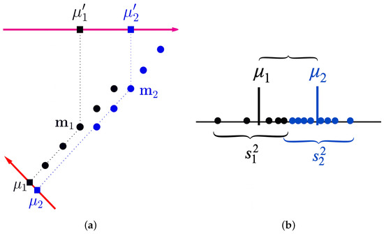
However, this criterion does not always work, as shown in Figure 1a. In other words, the distance between the means of the groups does not (always) guarantee the maximum possible separability between the groups.

Figure 1. Illustration of group separation criteria: (a) projection of group means along different axes; (b) between-group and within-group dispersion. Different colors correspond to different groups.

We need, in addition, to consider the variance within the groups, as shown in Figure 1b. We will calculate the value ${\theta }^{*}$ that maximizes the ratio of “between-groups variance” to “within-groups variance.” The difference between the means (in the new space) is yielded by the following equation:

$${\widehat{u}}_2-{\widehat{u}}_1={\theta }^T{u}_2-{\theta }^T{u}_1={\theta }^T\left(u_2-u_1\right)(\mathrm{between}-\mathrm{groups}\mathrm{variance})$$

(12)

Additionally, we define the within-groups variance using the following formulas:

$${\widehat{s}}_k^2=\sum _{j\in c_k}{\left(y^{\left(j\right)}-{\widehat{u}}_k\right)}^2,k=1,2$$

(13)

Thus, the objective function that we want to maximize is

$$J\left(\theta \right)={\displaystyle \frac{{\left({\widehat{u}}_2-{\widehat{u}}_1\right)}^2}{{\widehat{s}}_1^2+{\widehat{s}}_2^2}}$$

(14)

Maximizing this function aims to find a one-dimensional projection that clusters objects from the same group “tightly” together while simultaneously maximizing the distance between the group means of the projected values.

Let us analyze the quantity $J\left(\theta \right)$ using the following formulas:

$$\begin{array}{c}{\displaystyle S_k=\sum _{j\in c_k}\left(x^{\left(j\right)}-u_k\right){\left(x^{\left(j\right)}-u_k\right)}^T,k=1,2,}\hfill \\ S_w=S_1+S_2,S_B=\left(u_2-u_1\right){\left(u_2-u_1\right)}^T.\hfill \end{array}$$

(15)

Theorem 1

(Fisher’s Linear Discriminant for Two Groups). Assume that the within-groups scatter matrix $S_w$ is invertible. Then the vector ${\theta }^{*}$ that maximizes

$$J\left(\theta \right)={\displaystyle \frac{{\theta }^T{S}_B\theta }{{\theta }^T{S}_w\theta }}$$

(16)

is given, up to a nonzero multiplicative constant (normalization), by 

$${\theta }^{*}=S_w^{-1}(u_2-u_1).$$

(17)

Proof. 

The quantity:

$$\begin{array}{cc}\hfill {\widehat{s}}_k^2=\sum _{j\in c_k}{\left(y^{\left(j\right)}-{\widehat{u}}_k\right)}^2& =\sum _{j\in c_k}{\left({\theta }^T{x}^{\left(j\right)}-{\theta }^T{u}_k\right)}^2=\sum _{j\in c_k}{\left({\theta }^T\left(x^{\left(j\right)}-u_k\right)\right)}^2\hfill \\ \hfill & =\sum _{j\in c_k}{\theta }^T\left(x^{\left(j\right)}-u_k\right){\left(x^{\left(j\right)}-u_k\right)}^T\theta \hfill \\ \hfill & ={\theta }^T\left(\sum _{j\in c_k}\left(x^{\left(j\right)}-u_k\right){\left(x^{\left(j\right)}-u_k\right)}^T\right)\theta ={\theta }^T{S}_k\theta ,k=1,2\hfill \end{array}$$

(18)

Therefore, the denominator of $J\left(\theta \right)$, can be written as follows: ${\widehat{s}}_1^2+{\widehat{s}}_2^2={\theta }^T{S}_1\theta +{\theta }^T{S}_2\theta ={\theta }^T\left(S_1+S_2\right)\theta ={\theta }^T{S}_w\theta$ and moreover ${\left({\widehat{u}}_2-{\widehat{u}}_1\right)}^2={\left({\theta }^T{u}_2-{\theta }^T{u}_1\right)}^2={\left({\theta }^T\left(u_2-u_1\right)\right)}^2={\theta }^T\left(u_2-u_1\right){\left(u_2-u_1\right)}^T\theta ={\theta }^T{S}_B\theta$. Furthermore, $J\left(\theta \right)$ can take the following form: $J\left(\theta \right)={\displaystyle \frac{{\left({\widehat{u}}_2-{\widehat{u}}_1\right)}^2}{{\widehat{s}}_1^2+{\widehat{s}}_2^2}}={\displaystyle \frac{{\theta }^T{S}_B\theta }{{\theta }^T{S}_w\theta }}$. To compute its maximum, we differentiate it with respect to $\theta$ and set it equal to zero, yielding the following:

$$\begin{array}{cc}\hfill & {\displaystyle \frac{\partial J\left(\theta \right)}{\partial \theta }}={\displaystyle \frac{\partial }{\partial \theta }}\left({\displaystyle \frac{{\theta }^T{S}_B\theta }{{\theta }^T{S}_w\theta }}\right)=\left({\theta }^T{S}_w\theta \right){\displaystyle \frac{\partial {\theta }^T{S}_B\theta }{\partial \theta }}-\left({\theta }^T{S}_B\theta \right){\displaystyle \frac{\partial {\theta }^T{S}_w\theta }{\partial \theta }}\hfill \\ \hfill & =\left({\theta }^T{S}_w\theta \right)2S_B\theta -\left({\theta }^T{S}_B\theta \right)2S_w\theta =0\Rightarrow \hfill \\ \hfill & {\displaystyle \frac{{\theta }^T{S}_w\theta }{{\theta }^T{S}_w\theta }}{S}_B\theta -{\displaystyle \frac{{\theta }^T{S}_B\theta }{{\theta }^T{S}_w\theta }}{S}_w\theta =0\Rightarrow S_B\theta -J\left(\theta \right)S_w\theta =0\hfill \end{array}$$

(19)

If the matrix $S_w$ is invertible, we take

$$\begin{array}{cc}\hfill & S_w^{-1}{S}_B\theta -J\left(\theta \right)S_w^{-1}{S}_w\theta =0\Rightarrow J\left(\theta \right)\theta =S_w^{-1}{S}_B\theta \hfill \\ \hfill & \Rightarrow J\left(\theta \right)\theta =S_w^{-1}\left(u_2-u_1\right)\underset{c\in \mathbb{R}}{\underbrace{{\left(u_2-u_1\right)}^T\theta }}\hfill \\ \hfill & \Rightarrow J\left(\theta \right)\theta =c{S}_w^{-1}\left(u_2-u_1\right)\Rightarrow \theta ={\displaystyle \frac{c}{J}}{S}_w^{-1}\left(u_2-u_1\right)\hfill \end{array}$$

(20)

Thus, ${\theta }^{*}=S_w^{-1}\left(u_2-u_1\right)$ (after appropriate normalization).    □

Remark 3.

An alternative way of determining ${\theta }^{*}=S_w^{-1}\left(u_2-u_1\right)$, is based on the following:

(I) 

The matrix $S_B$ is square, symmetric, and positive semi-definite, $rank\left(S_B\right)=1$, i.e., it has only one positive eigenvalue.

(II) 

The matrix $S_w$ is square, symmetric and positive semi-definite.

(III) 

Theorem: Suppose the matrix $S_w$ is non-singular. The direction that maximizes our problem is given by the eigenvector corresponding to the largest eigenvalue of the (generalized) eigenvalue problem:

$$S_w^{-1}{S}_B{v}_1={\lambda }_1{v}_1$$

(21)

2.8.2. Classification Accuracy—Classification Table

Although researchers apply LDA for predicting the classification of new observations (whose group membership is unknown), we can also use it to assess the accuracy/correctness of the classification process. We are interested in the percentage of observations that are classified correctly (hit ratio), which is an indirect and intuitive measure of the degree of separability between groups (see Table 1). It is calculated using the confusion matrix (classification, confusion, or prediction table) and is equal to the sum of the diagonal elements of the matrix divided by the total size of the dataset ${\displaystyle \frac{{\sum }_{i=1}^p{\alpha }_{ii}}{n}}$ [34,35].

Table 1. Classification (confusion) table in LDA.

Classification table		Prediction (with LDA)
		Class 1	Class 2	…	Class p
Initial classes	Class 1	${\alpha }_{11}$	${\alpha }_{12}$	…	${\alpha }_{1p}$
	Class 2	${\alpha }_{21}$	${\alpha }_{22}$	…	${\alpha }_{2p}$
	⋮	⋮	⋮	⋱	⋮
	Class p	${\alpha }_{p1}$	${\alpha }_{p2}$	…	${\alpha }_{pp}$

The percentage mentioned should be compared with the expected percentage of correct classification if the distribution of cases among groups was random (e.g., $50\%$ in the case of two groups, $25\%$ in the case of four groups). However, this percentage overestimates the power of the classification process because its evaluation is based on the same observations used to construct the discriminant functions.

When the sample size is large for classification evaluation, it is divided into two subsets: one for constructing the discriminant functions (training sample) and the other for validating the (correct) classifications (validation sample). Although there is disagreement about the size of these subsets, the one used for computing the discriminant functions should be sufficiently large to ensure the stability of the function coefficients. A special case of dividing the sample is cross-validation: one observation is withheld at each iteration, the discriminant functions are constructed, and then the group to which it belongs is estimated [5,32]. The process is repeated for each observation, and in the end, the percentage of correctly classified observations is calculated.

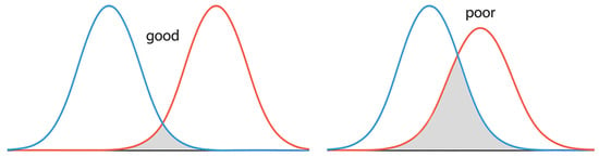
Alternatively, a second graphical way to assess the accuracy/validity of the classification process is as follows: at the end of applying the discriminant analysis, it is assumed that the discriminant scores (regarding each discriminant function) follow the normal distribution. The degree of overlap of these distributions can be used as a measure of the degree of correct classification of observations (Figure 2).

Figure 2. Distributions of discriminant scores for assessing classification overlap between groups.

2.9. Problems with the Implementation of Discriminant Analysis—Violation of Assumptions

To apply LDA to a dataset, certain key assumptions need to be satisfied, including the multivariate normal distribution (MND) and equality of covariance matrices (within groups). Violating these assumptions has the following consequences:

(I)

Multivariate Normal Distribution

(a)

Significance test: In this approach, we compare the theoretical distribution of a statistic calculated under the assumption of a multivariate normal distribution (MND) of the population with its actual sampling distribution. If this assumption is violated, discrepancies will arise between the two distributions. Although Linear Discriminant Analysis (LDA) is robust to minor deviations from normality, the accuracy and validity of the results may still be affected.

(b)

Chi-square distribution: Normality is also essential when classifying observations based on their probabilities of group membership. These probabilities are derived under multivariate normality; under this assumption, the associated squared Mahalanobis distances follow a chi-square distribution. If this assumption is not satisfied, the resulting probabilities will be inaccurate, leading to suboptimal classification and an increased rate of misclassification.

(II)

Equality of Covariance Matrices

When the within-group covariance matrices are unequal, distortions arise in both the discriminant and classification functions. The main source of error is the within-group covariance matrix W, which can no longer be used to simplify the discriminant functions when this assumption is violated. Consequently, the discriminant functions fail to maximize group separation, and the membership probabilities become biased to some extent. One way to address this issue is to incorporate the individual group covariance matrices into the probability calculations, as performed in quadratic discriminant analysis.

The difficulty with violating these assumptions lies in the uncertainty about the degree of violation that is acceptable for the analysis to remain valid. In such situations, indirect methods can be used to estimate the extent of violation by examining statistics that do not rely on these assumptions. Specifically:

(i)

When deciding the number and significance of discriminant functions, researchers commonly rely on Wilks’s lambda or its associated chi-square test, both of which depend heavily on the validity of underlying assumptions. Alternatively, canonical correlations or the percentage of relative significance can be used. If these values are low, the discriminant analysis may lack practical importance, even if statistically significant. Significance tests are especially crucial with small sample sizes, where assumption violations warrant careful consideration [23].

(ii)

In classification, difficulties occur when membership probabilities are close to each other. For instance, if an observation has a 0.51 probability of belonging to Group 1 and 0.49 to Group 2, minor errors from assumption violations can easily cause misclassification.

Additionally, several challenges arise when applying LDA:

(i)

The number of discriminant axes may be insufficient to accurately classify a substantial portion of the data.

(ii)

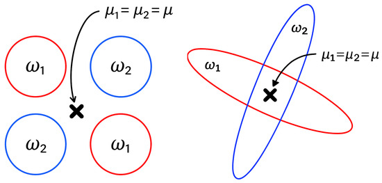
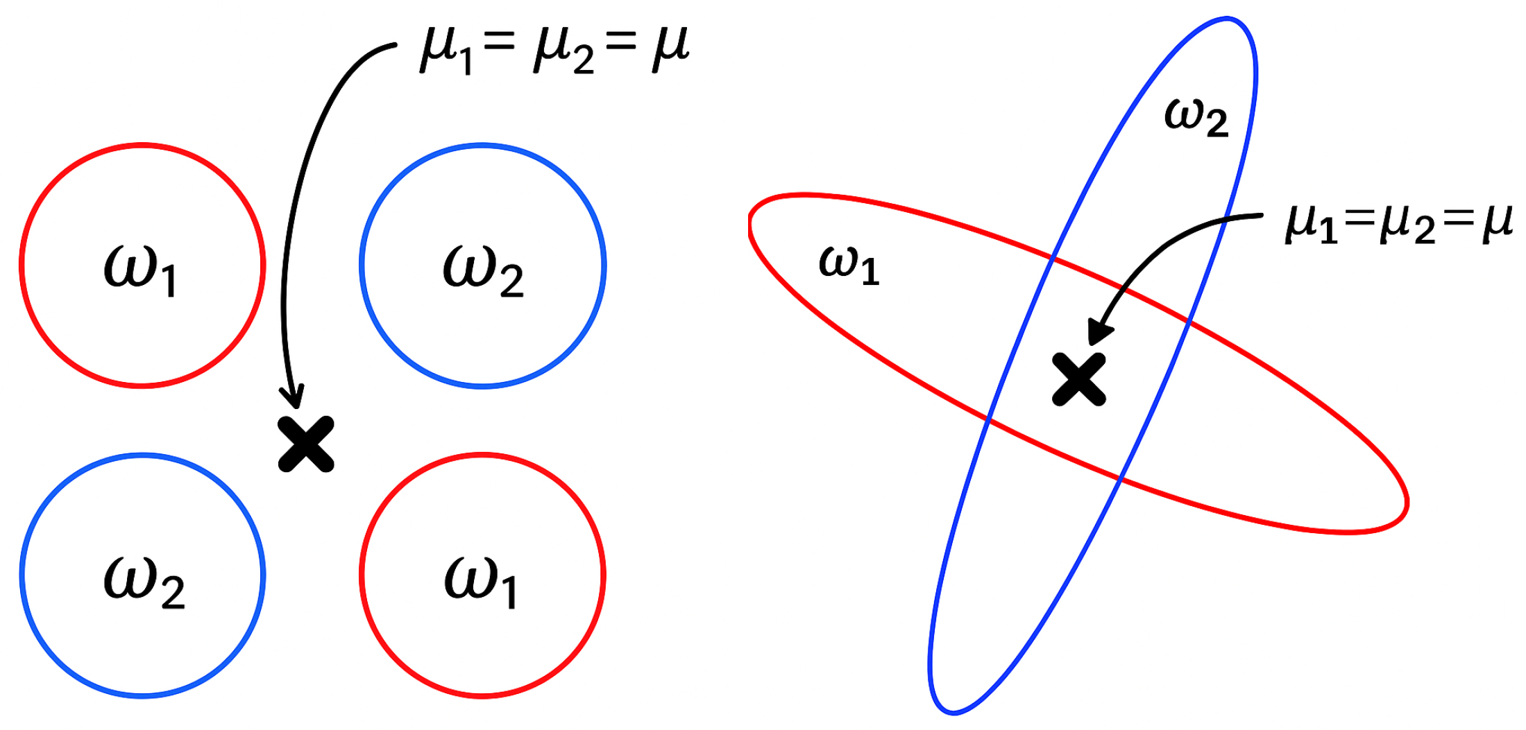
LDA may fail to capture complex data structures essential for accurate classification, particularly in cases where group means are similar but covariance structures differ.

(iii)

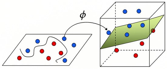
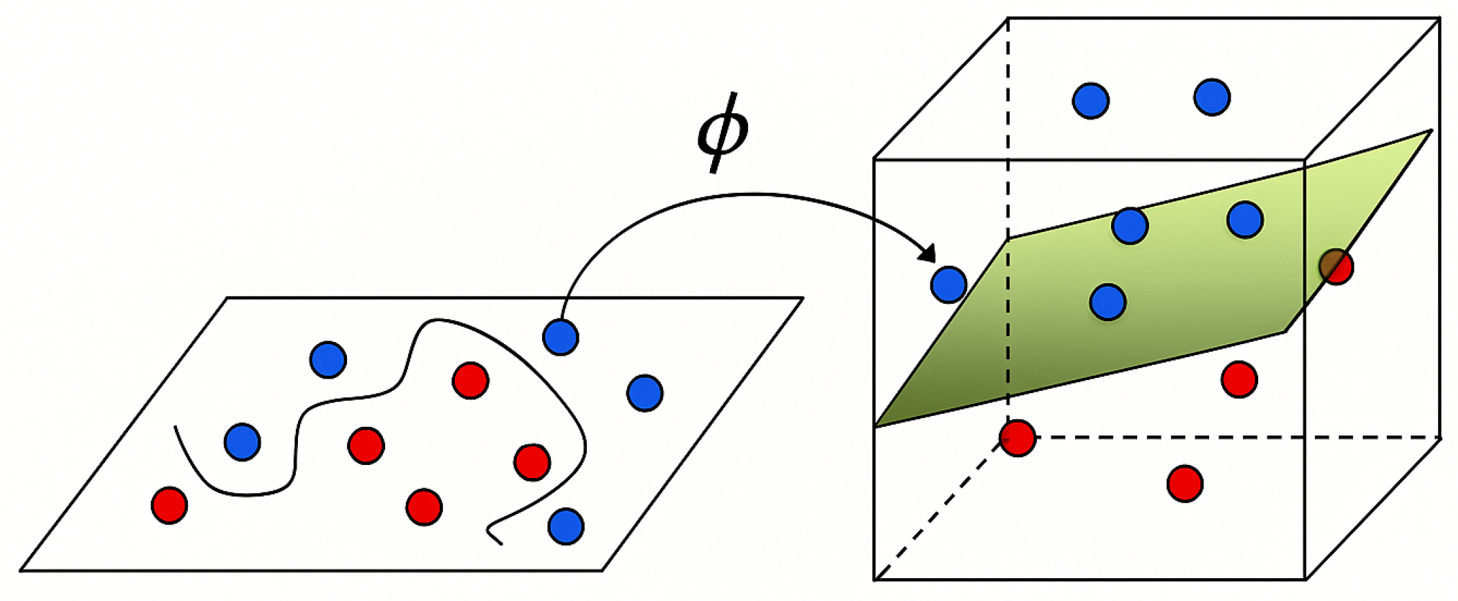
LDA can be ineffective when groups are not linearly separable; that is, when the discriminative information lies in differences in variance rather than in the means (see Figure 3). In such situations, Kernel Discriminant Analysis (K.D.A.) is used [37,38]. K.D.A. applies a nonlinear transformation that maps the data into a higher-dimensional space where they become linearly separable, allowing discriminant analysis to be performed effectively in this new space (see Figure 4).

Figure 3. Example of groups that are not linearly separable in the original feature space.

Figure 4. Visualization of nonlinearly separable groups in higher-dimensional space.

3. Case Study: Implementation of LDA in a Medical Context

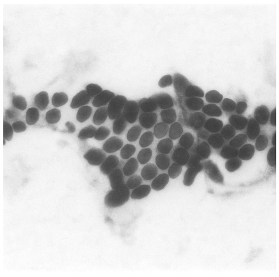
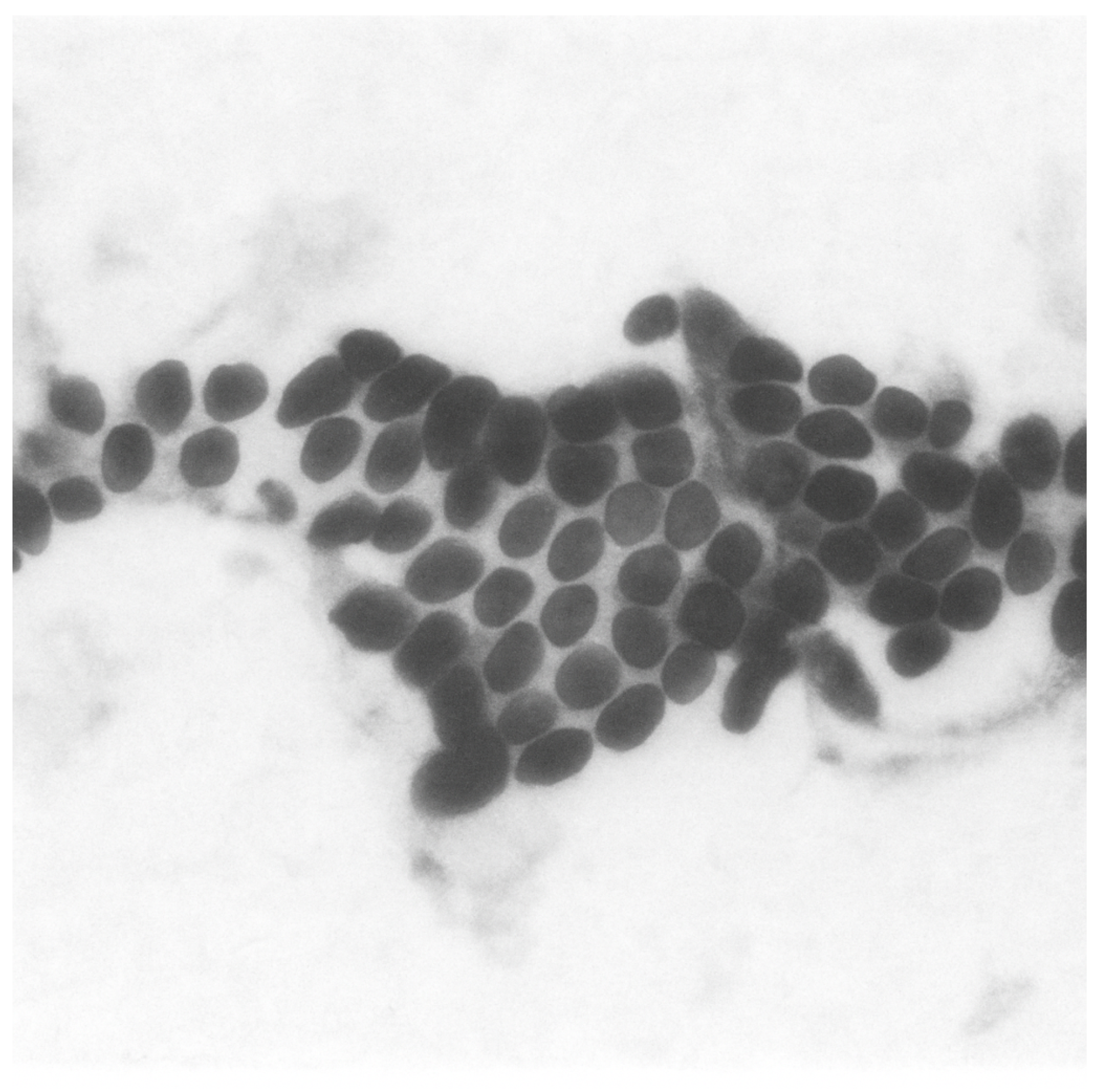
In this study, we examine the implementation of LDA in the context of clinical diagnostics, using the “Breast Cancer Wisconsin (Diagnostic)” dataset, originally compiled by Dr. William H. Wolberg et al. at the University of Wisconsin–Madison and publicly available via the UCI Machine Learning Repository [39]. It consists of digitized images derived from fine needle aspirates (FNA) of breast masses (see Figure 5), processed to extract numerical features that characterize the morphology of cell nuclei present in the samples. Each case corresponds to one patient and includes a label indicating whether the tumor is benign (labeled 0) or malignant (labeled 1), stored in the column diagnosis.

Figure 5. Representative breast mass image from which morphological features were extracted.

For each nucleus, ten real-valued features were calculated:

• Radius (mean distance from the center to points on the perimeter);
• Texture (standard deviation of gray-scale values);
• Perimeter;
• Area;
• Smoothness (local variation in radius lengths);
• Compactness (perimeter²/area $-1.0$);
• Concavity (severity of concave portions of the contour);
• Concave points (number of concave portions of the contour);
• Symmetry;
• Fractal dimension (“coastline approximation”).

For each of the above features, three statistical summaries were computed: the mean, the standard error, and the “worst” value (defined as the mean of the three largest values for that feature) named radius mean, radius_se, radius_worst, respectively. This results in a total of 30 features per sample. The dataset consists of 569 observations in total, with 357 labeled as benign and 212 as malignant. Although in our dataset all diagnostic labels are known, in cases where the disease status is partially missing (verification bias), estimation techniques such as the semiparametric and shrinkage-based approaches of Ahmed et al. [40] can be applied to recover diagnostic information reliably.

Given the binary classification nature of the problem (benign vs. malignant), LDA is a suitable method for modeling the class separability based on these quantitative features.

3.1. Data Preprocessing

Before applying LDA, a thorough preprocessing phase is essential, particularly due to the assumption that LDA performs optimally when input variables follow a normal distribution. The majority of the 30 features failed the Kolmogorov–Smirnov (K-S) test, suggesting that the assumption of normality does not hold for most variables in their original form. To further examine distributional properties, skewness and kurtosis values are assessed [41,42]. Ideally, skewness values should fall between −1 and +1, and kurtosis near 3. While some variables (e.g., radius mean, smoothness_mean) are within acceptable limits, others exhibited significant skewness or peakedness, confirming the need for transformation. To address these issues and enhance normality, a Box–Cox transformation is applied to all variables [2], yielding the following:

$$y^{\left(\lambda \right)}=\left\{\begin{array}{cc}{\displaystyle \frac{y^{\lambda }-1}{\lambda }}\hfill & \mathrm{if}\lambda \ne 0\hfill \\ lny\hfill & \mathrm{if}\lambda =0\hfill \end{array}\right.$$

(22)

The Box–Cox transformation requires strictly positive data $(\mathrm{y}>0)$. The parameter $\lambda$ is estimated from the data by maximizing the log-likelihood function, with the optimal $\lambda$ corresponding to the value that provides the best model fit.

Effect of the Box–Cox Transformation on Feature Skewness

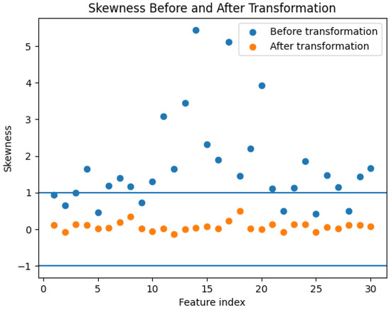
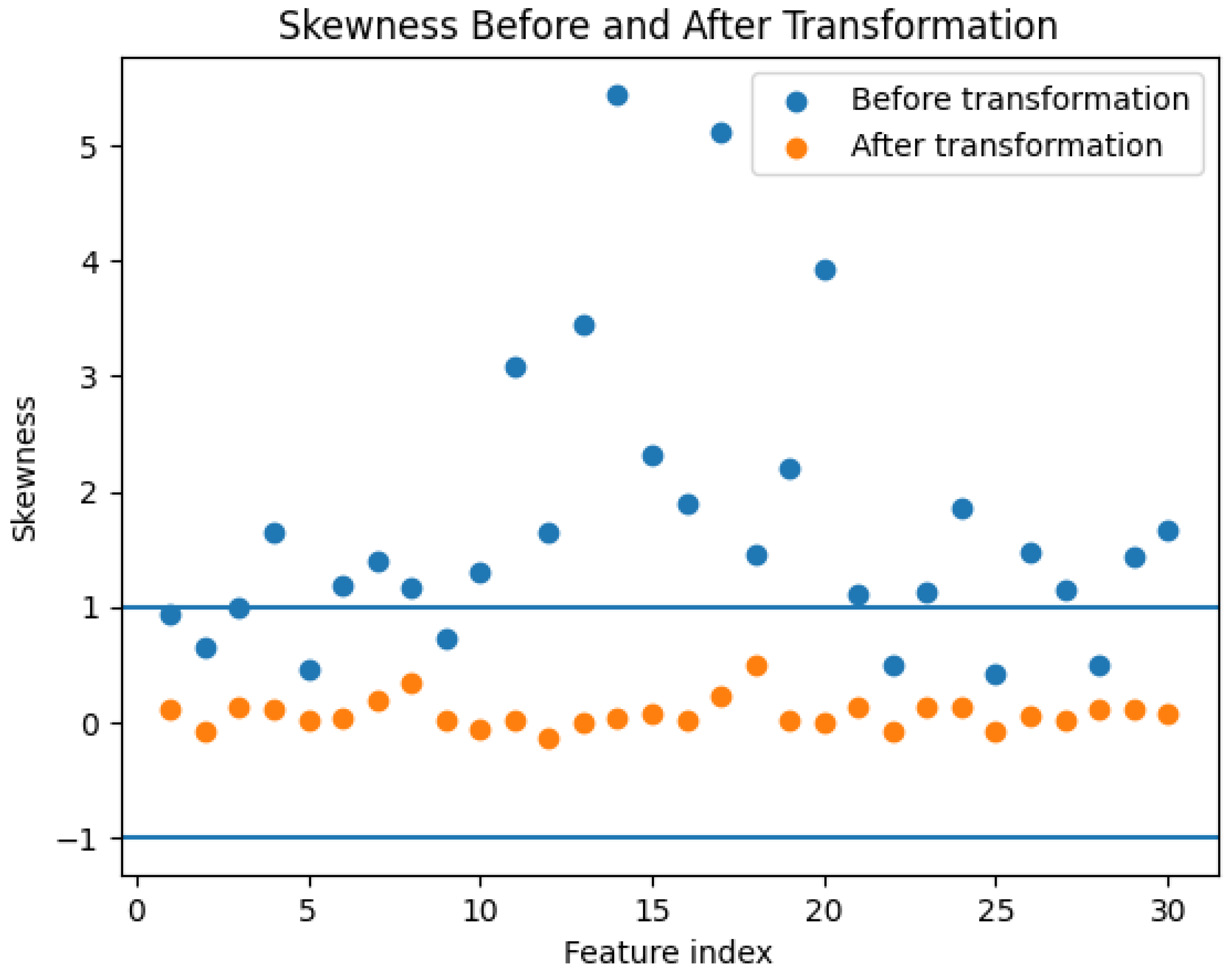
In the present dataset, the sample skewness of the original features ranges from moderate values (approximately $0.4$) up to strongly skewed cases exceeding 5, indicating substantial departures from symmetry for several variables. For a real-valued feature X with mean $\mu$ and standard deviation $\sigma$, the (Fisher–Pearson) skewness coefficient is defined as

$${\gamma }_1\left(X\right)={\displaystyle \frac{\mathbb{E}\left[{(X-\mu )}^3\right]}{{\sigma }^3}}.$$

(23)

For right-skewed features (${\gamma }_1\left(X\right)>0$), the application of a monotone transformation $Y=g\left(X\right)$, such as the logarithmic or Box–Cox transformation, compresses the right tail of the distribution relative to the left tail. This reduces the contribution of extreme values to the third central moment and, consequently, decreases the magnitude of the skewness coefficient. After transformation, the skewness of all features is substantially reduced and concentrated within a narrow interval close to zero, with all values lying in the range $[-0.15,0.49]$, confirming improved distributional symmetry across the entire feature set. The effect of the Box–Cox transformation on feature skewness is summarized in Figure 6.

Figure 6. Feature-wise skewness before and after the Box–Cox transformation. Horizontal reference lines at $\pm 1$ indicate the commonly accepted bounds for approximately symmetric distributions. After transformation, the skewness of all features lies within this interval.

In practice, statistical software packages (R 4.x, Python 3.x, SPSS 27, and SAS 9.4) perform this procedure automatically and report $\lambda$ along with a confidence interval. The transformation is particularly useful in stabilizing variance and making the data more closely resemble a normal distribution. The transformed variables are then re-evaluated, confirming improved distributional properties suitable for LDA modeling. Next, we standardize all features to ensure comparability of scales and to aid in outlier detection. To identify and potentially exclude outliers, we apply the rule $\left|\mathrm{Z}\right|<3$, which retains values within three standard deviations of the mean. After removing the outliers, the remaining dataset consists of 538 observations: 338 labeled as benign and 200 as malignant. This dataset is used for all subsequent modeling. Then, we run discriminant analysis, using SPSS software, v27 [43]. For reproducibility purposes, all tables and figures reported in this study are generated directly from SPSS output.

Although the analyses in this paper are conducted using SPSS, the same Linear Discriminant Analysis (LDA) methodology is readily available in other commonly used statistical platforms, including open-source environments. In Minitab, LDA can be performed via the Discriminant Analysis procedure (Stat → Multivariate → Discriminant Analysis), which provides classification functions, posterior probabilities, and misclassification summaries in a structured, menu-driven environment. In R, LDA is implemented through the lda function of the MASS package, following the classical Fisher framework and allowing direct access to group means, pooled covariance matrices, and discriminant coefficients [44]. In Python, the LinearDiscriminantAnalysis class in the scikit-learn library offers an efficient implementation with options for different solvers and covariance regularization, and integrates naturally with preprocessing and validation tools [45]. These observations indicate that the SPSS-based workflow adopted in this study is fully consistent with, and transferable to, other established statistical software platforms.

3.2. Tests of Equality of Group Means

Table 2, “Tests of Equality of Group Means”, presents the results of a series of univariate ANOVAs conducted on each of the standardized and transformed predictor variables, using the diagnostic outcome (benign vs. malignant) as the grouping factor. This step serves as an initial assessment of whether significant differences exist between the two groups for each independent variable and, consequently, whether the variables have discriminatory values. Similar insights into group separation can also be obtained from the descriptive ”Group Statistics” table provided by SPSS, based on group means and standard deviations.

Table 2. Univariate ANOVA results assessing group differences between benign and malignant cases for each predictor.

Tests of Equality of Group Means
	Wilks’ Lambda	F	df1	df2	Sig.
radius_mean	0.468	609.802	1	536	0.000
texture_mean	0.811	125.030	1	536	0.000
perimeter_mean	0.447	664.430	1	536	0.000
area_mean	0.464	618.963	1	536	0.000
smoothness_mean	0.873	78.111	1	536	0.000
compactness_mean	0.644	295.858	1	536	0.000
concavity_mean	0.467	610.864	1	536	0.000
concavepoints_mean	0.385	857.109	1	536	0.000
symmetry_mean	0.889	67.147	1	536	0.000
fractal_dimension_mean	0.997	1.874	1	536	0.172
radius_se	0.607	346.413	1	536	0.000
texture_se	0.998	0.830	1	536	0.363
perimeter_se	0.602	354.119	1	536	0.000
area_se	0.486	566.676	1	536	0.000
smoothness_se	0.997	1.373	1	536	0.242
compactness_se	0.874	77.485	1	536	0.000
concavity_se	0.826	113.127	1	536	0.000
concavepoints_se	0.798	135.383	1	536	0.000
symmetry_se	0.995	2.670	1	536	0.103
fractal_dimension_se	0.968	17.925	1	536	0.000
radius_worst	0.386	851.722	1	536	0.000
texture_worst	0.782	149.464	1	536	0.000
perimeter_worst	0.373	902.924	1	536	0.000
area_worst	0.386	853.907	1	536	0.000
smoothness_worst	0.822	115.914	1	536	0.000
compactness_worst	0.645	294.414	1	536	0.000
concavity_worst	0.533	470.237	1	536	0.000
concavepoints_worst	0.386	854.044	1	536	0.000
symmetry_worst	0.827	112.058	1	536	0.000
fractal_dimension_worst	0.904	57.242	1	536	0.000

Accordingly, Table 2 includes Wilks’ Lambda values, F-statistics, degrees of freedom, and significance levels. A lower Wilks’ Lambda and higher F-value, alongside a significance value (Sig.) below 0.05, indicate that a variable contributes meaningfully to the differentiation between groups. Here, most of the variables are statistically significant (Sig. $=0.000$), suggesting they are strong candidates for inclusion in the LDA model. Specifically, variables such as concavepoints_mean, perimeter_worst, radius_worst, and concavepoints_worst show particularly low Wilks’ Lambda values (around 0.37–0.39) and extremely high F-values (above 850), indicating strong group separation. On the other hand, a small subset of variables—including fractal_dimension_mean (Sig. = 0.172), texture_se (Sig. = 0.363), smoothness_se (Sig. = 0.242), and symmetry_se (Sig. $=0.103$)—did not show statistically significant differences between groups (and may therefore be excluded from the final discriminant model). In summary, the significant group differences observed across most variables confirm their value as discriminators between benign and malignant cases, validating the application of LDA in this study.

3.3. Assessment of Homogeneity of Covariance Matrices (Box’s M Test)

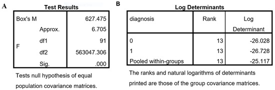
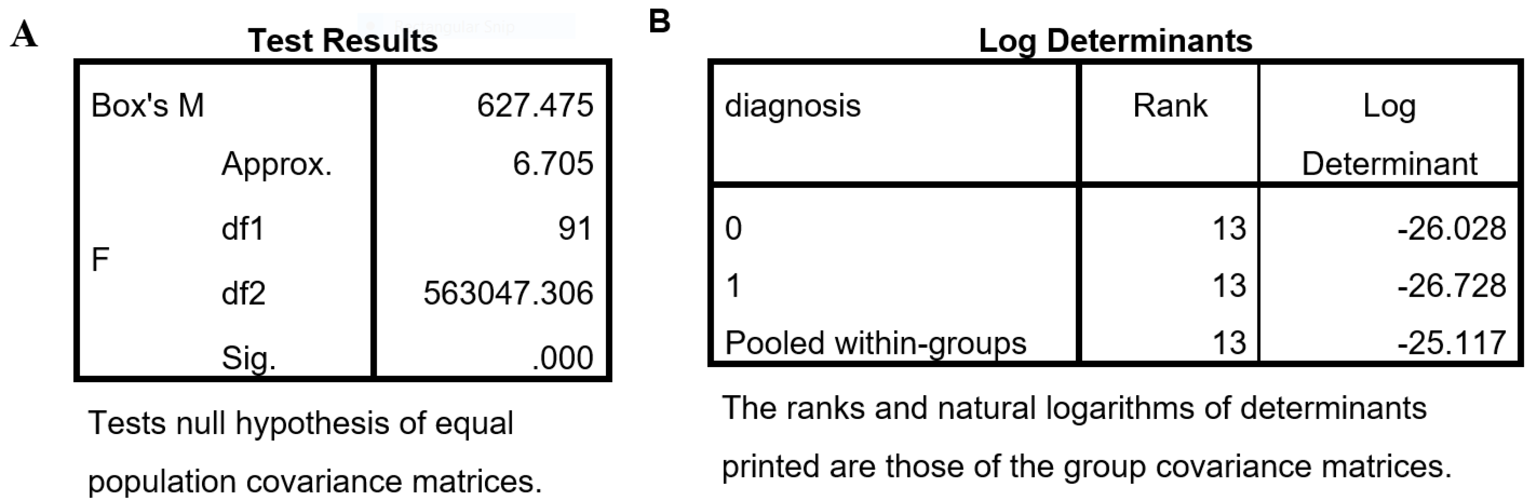
The Box’s M test is used (Figure 7A) to evaluate the assumption of homogeneity of covariance matrices across groups (benign vs. malignant). The test examines the null hypothesis that the population covariance matrices are equal [3]. In the current analysis, it yielded Box’s $M=627.475$ and a significance level of $p<0.001$; thus, the null hypothesis is rejected, indicating that the assumption of equal covariance matrices is not satisfied. However, Box’s M test is known to be extremely sensitive to deviations from multivariate normality and large sample sizes, often resulting in significant outcomes even when the practical violation is minimal [16]. Therefore, a significant Box’s M test does not necessarily invalidate the use of LDA.

Figure 7. Results of (A) Box’s M test and (B) logarithms of the determinants of the group covariance matrices for assessing the equality of population covariance matrices.

An alternative approach is to examine the logarithms of the determinants of the group covariance matrices (Figure 7B). The log determinant for group 0 is $-26.028$, for group 1$-26.728$, and for the pooled within-groups matrix $-25.117$. The small difference $(\sim$0.7) between the determinants suggests that the covariance structures do not differ substantially, a fact that supports the argument that the assumption of homogeneity is not severely violated in practice [34].

3.4. Assessment of Multicollinearity (Tolerance Test)

Table 3, “Variables Failing Tolerance Test”, reports the within-groups variance and corresponding tolerance values for each predictor variable used in the discriminant analysis. The tolerance statistic is a measure of multicollinearity and reflects the degree to which a given independent variable is linearly related to the other predictors. A tolerance value close to zero indicates high multicollinearity, which may distort the estimation of discriminant functions and reduce the reliability of the model [16]. In this analysis, several variables exhibited low tolerance values, as shown in Table 3, raising concerns, for example, radius_worst (0.045), texture_worst (0.042), area_worst (0.040), and perimeter_worst (0.049). It is common practice to remove these variables from subsequent analyses. Accordingly, SPSS automatically excluded 17 variables from the discriminant model.

Table 3. Multicollinearity diagnostics for predictor variables based on tolerance statistics.

Variables Failing Tolerance Test a
	Within-Groups Variance	Tolerance	Minimum Tolerance
compactness_mean	0.589	0.081	0.001
concavity_mean	0.383	0.148	0.001
radius_se	0.605	0.439	0.001
perimeter_se	0.596	0.425	0.001
area_se	0.484	0.365	0.001
compactness_se	0.807	0.247	0.001
concavity_se	0.581	0.292	0.001
fractal_dimension_se	0.909	0.286	0.001
radius_worst	0.357	0.045	0.001
texture_worst	0.748	0.042	0.001
perimeter_worst	0.343	0.049	0.001
area_worst	0.357	0.040	0.001
compactness_worst	0.585	0.182	0.001
concavity_worst	0.443	0.248	0.001
concavepoints_worst	0.312	0.080	0.001
symmetry_worst	0.699	0.119	0.001
fractal_dimension_worst	0.843	0.144	0.001

All variables passing the tolerance criteria are entered simultaneously. ^a Minimum tolerance level is 0.001.

3.5. Model Interpretation

(A)

Eigenvalues

Table 4, “Eigenvalues”, provides information about the discriminant function(s) derived from LDA. Since the dataset includes only two groups (benign and malignant), only one discriminant function is produced; therefore, the table reports a single eigenvalue. To this end, the eigenvalue $\lambda =3.022>1$ indicates a strong discriminating power of the function, explaining 100% of the discriminant variance in the model (since only one discriminant function is used). The canonical correlation coefficient of 0.867 shows a strong relationship between the discriminant scores and the diagnostic groups. The square of the canonical correlation $\left(0.{867}^2=0.751\right)$ shows that approximately $75.1\%$ of the variance in the dependent variable is explained by the model. This result reflects a strong discriminative ability between benign and malignant tumors.

Table 4. Eigenvalue and canonical correlation associated with the extracted discriminant function.

Eigenvalues
Function	Eigenvalue	% of Variance	Cumulative %	Canonical Correlation
1	3.022 a	100.0	100.0	0.867

^a First 1 canonical discriminant functions were used in the analysis.

(B)

Wilks’ Lambda—Significance of the Discriminant Function

The Wilks’ Lambda test is used to evaluate the overall statistical significance of the discriminant function derived from the analysis. It measures the proportion of total variance that is not accounted for by differences among groups. A lower Wilks’ Lambda value indicates that a greater proportion of the variance is explained by group differences, suggesting a stronger discriminative ability of the function.

In this analysis, Wilks’ Lambda is 0.249, with an associated chi-square value of 737.012, 13 degrees of freedom, and a significance level (Sig.) of $p<0.001$ (see Table 5). These values confirm that the discriminant function is highly significant and effectively differentiates between the two diagnostic categories (benign and malignant). Specifically, a Lambda of 0.249 suggests a strong separation between groups, consistent with approximately $75.1\%$ of the discriminant variance explained by group membership, indicating a strong model fit. This result is consistent with the high canonical correlation reported earlier ($\mathrm{r}=0.867$), further validating the effectiveness of the model in capturing the variance related to the classification task.

Table 5. Overall significance test of the discriminant function based on Wilks’ Lambda.

Wilks’ Lambda
Test of Function(s)	Wilks’ Lambda	Chi-Square	df	Sig.
1	0.249	737.012	13	0.000

(C)

Canonical Discriminant Function Coefficients—Construction of the Discriminant Function

Table 6, “Canonical Discriminant Function Coefficients”, presents the unstandardized coefficients used to construct the linear discriminant function. These coefficients function similarly to those in a regression model, forming a linear equation that best separates the two groups based on the predictor variables included. The sign and magnitude of the coefficients indicate the direction and the relative strength of each predictor’s role in distinguishing between the groups. Based on Table 6, the estimated discriminant function includes 13 variables and can be written as:

$$\begin{array}{cc}\hfill D=-10.812& \times \mathrm{radius}\_\mathrm{mean}+0.339\times \mathrm{texture}\_\mathrm{mean}-2.663\times \mathrm{perimeter}\_\mathrm{mean}\hfill \\ \hfill & + 14.061\times \mathrm{area}\_\mathrm{mean}-0.465\times \mathrm{smoothness}\_\mathrm{mean}\hfill \\ \hfill & + 1.329\times \mathrm{concavepoints}\_\mathrm{mean}+0.203\times \mathrm{symmetry}\_\mathrm{mean}\hfill \\ \hfill & - 0.002\times \mathrm{fractal}\_\mathrm{dimension}\_\mathrm{mean}+0.015\times \mathrm{texture}\_\mathrm{se}\hfill \\ \hfill & - 0.277\times \mathrm{smoothness}\_\mathrm{se}-0.061\times \mathrm{concavepoints}\_\mathrm{se}\hfill \\ \hfill & + 0.169\times \mathrm{symmetry}\_\mathrm{se}+0.893\times \mathrm{smoothness}\_\mathrm{worst}-0.089\hfill \end{array}$$

(24)

Table 6. Estimated coefficients of the linear discriminant function used for group separation.

Canonical Discriminant Function Coefficients
	Function
	1
radius_mean	−10.812
texture_mean	0.339
perimeter_mean	−2.663
area_mean	14.061
smoothness_mean	−0.465
concavepoints_mean	1.329
symmetry_mean	0.203
fractal_dimension_mean	−0.002
texture_se	0.015
smoothness_se	−0.277
concavepoints_se	−0.061
symmetry_se	0.169
smoothness_worst	0.893
(Constant)	−0.089
Unstandardized coefficients

The variables with the highest absolute values of coefficients, such as area_mean (14.061), radius_mean (−10.812), and perimeter_mean (−2.663), appear to make the strongest contribution to group separation, highlighting their importance in the model. This equation is used to compute discriminant scores for each case, which are then used for group classification.

(D)

Functions at Group Centroids - Interpretation

Table 7, “Functions at Group Centroids”, presents the average discriminant scores for each of the two diagnostic groups: 0 (benign) and 1 (malignant). The scores are calculated by inserting the mean values of the independent variables for each group into the discriminant function equation. In our case, the centroid for the benign group (0) is $-1.335$, while for the malignant group (1), it is $2.256$.

Table 7. Mean discriminant scores (centroids) for benign and malignant diagnostic groups.

Functions at Group Centroids
Diagnosis	Function
	1
0	−1.335
1	2.256
Unstandardized canonical discriminant functions evaluated at group means

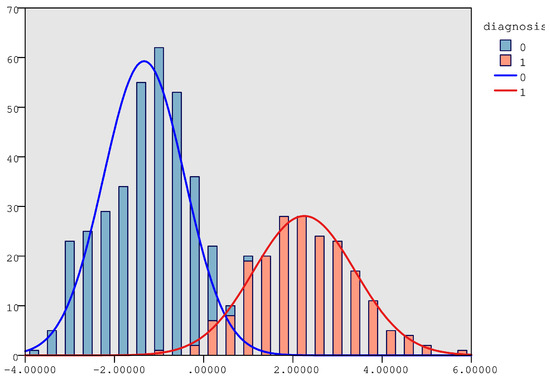
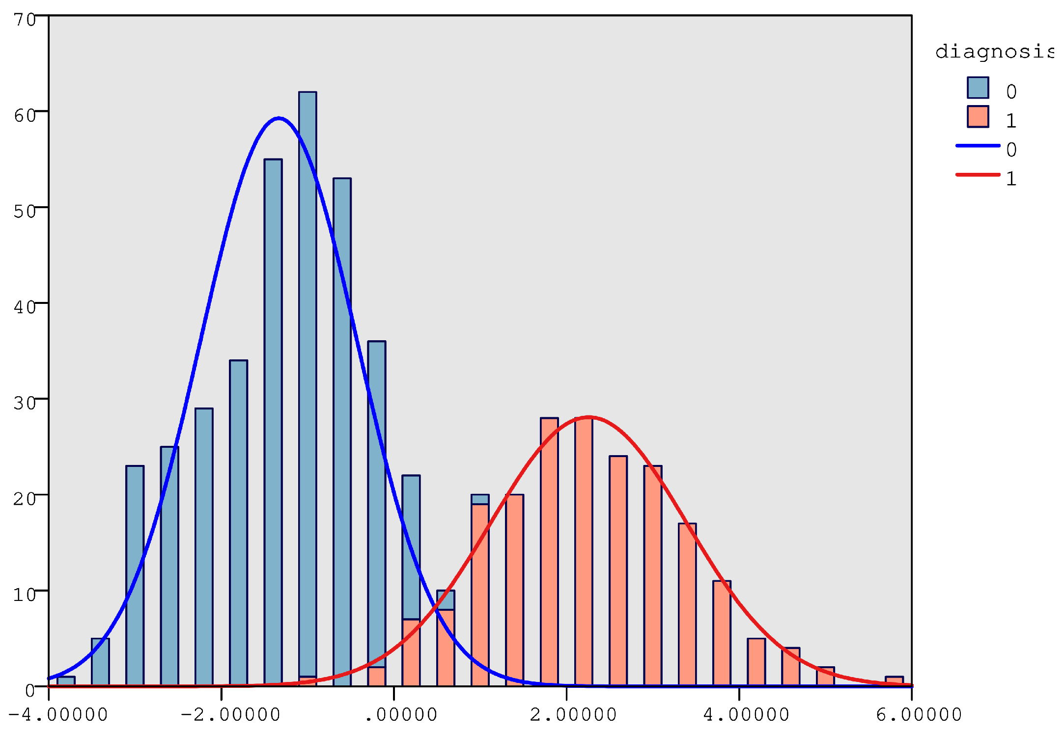
As illustrated by Figure 8, these scores lie on opposite sides of the discriminant axis and are far apart, which suggests a strong separation between the two groups. As can be seen, the clear distance between these two centroids supports the model’s high classification ability and confirms that the discriminant function effectively distinguishes between the two categories of the dependent variable. Cases with discriminant scores closer to −1.335 are predicted to belong to the benign group, whereas cases closer to 2.256 are classified as malignant.

Figure 8. Distribution of discriminant scores along the extracted discriminant function. Diagnosis: 0: the tumor is benign; 1: the tumor is malignant.

(E)

Classification Results—Accuracy

Table 8, “Classification Results”, summarizes the performance of the discriminant function in predicting group membership for the dependent variable (diagnosis: benign vs. malignant).

Table 8. Classification performance of the linear discriminant model for original and cross-validated samples.

Classification Results a,c
		Diagnosis	Predicted Group Membership		Total
			0	1
Original	Count	0	336	2	338
		1	10	190	200
	%	0	99.4	0.6	100.0
		1	5.0	95.0	100.0
Cross-validated b	Count	0	335	3	338
		1	11	189	200
	%	0	99.1	0.9	100.0
		1	5.5	94.5	100.0

a. 97.8% of original grouped cases correctly classified. b. Cross-validation is performed only for those cases in the analysis. In cross-validation, each case is classified by the functions derived from all cases other than that case. c. 97.4% of cross-validated grouped cases correctly classified.

Original Classification

The analysis correctly classified $97.8\%$ of the original grouped cases. Specifically, 336 out of 338 benign cases ($99.4\%$) and 190 out of 200 malignant cases ($95.0\%$) were correctly classified, indicating high predictive accuracy. The diagonal values in the table represent correct classifications, while off-diagonal values indicate misclassifications. This high classification accuracy reflects the strong discriminating power of the model.

Cross-Validation (Leave-One-Out Method)

To assess the model’s generalizability, cross-validation was performed using the leave-one-out technique. In this method, each case is classified by the discriminant function derived from all other cases except the one being classified. The cross-validated accuracy remained high, with $97.4\%$ of the grouped cases correctly classified ($99.1\%$ for benign and $94.5\%$ for malignant cases). This slight decrease from the original classification accuracy suggests a robust model with minimal overfitting.

(F)

Prior Probabilities—Interpretation and Model Accuracy

Table 9, “Prior Probabilities for Groups”, presents the assumed likelihood of each group membership before the discriminant analysis is conducted. These priors are based on the observed proportions in the sample: $62.8\%$ of cases belong to group 0 (benign), while $37.2\%$ belong to group 1 (malignant). These proportions are used in the classification process to reflect the unequal group sizes and to avoid bias in favor of the larger group.

Table 9. Prior group membership probabilities used in the discriminant classification procedure.

Prior Probabilities for Groups
Diagnosis	Prior	Cases Used in Analysis
		Unweighted	Weighted
0	0.628	338	338.000
1	0.372	200	200.000
Total	1.000	538	538.000

An important aspect of interpreting discriminant analysis is assessing the hit ratio, which reflects the model’s classification accuracy [16,34,40]. To determine whether the hit ratio is acceptable, it must be compared against a baseline—the level of accuracy that would be expected by chance alone. In the case of two groups with equal sizes, a random assignment would yield an accuracy of $50\%$. However, when group sizes are unequal, the chance hit ratio corresponds to the proportion of the largest group, in this case, $62.8\%$. As a rule of thumb, most researchers consider the model acceptable if its hit ratio exceeds the chance level by at least $25\%$. Thus, in this case, a hit ratio above $78.5\%(62.8\%\times 1.25)$ would be considered acceptable. The predictor model developed in this study clearly surpasses this threshold.

(G)

Model Dimensionality Reduction and Classification Accuracy

As an additional approach, the stepwise discriminant analysis method was applied and reduced the initial set of 30 predictor variables to 10 statistically significant ones, effectively addressing the dimensionality of the problem and improving model interpretability. As observed in Table 10 (Wilks’ Lambda), each additional variable entered into the model led to a successive decrease in the Lambda value, with the last step 14 yielding a Wilks’ Lambda of $0.229$. This consistent reduction, along with the highly significant F-statistics ($p<0.001$ at each step), confirms that the selected variables contribute meaningfully to group discrimination.

Table 10. Stepwise evolution of Wilks’ Lambda as predictor variables are sequentially entered into the discriminant model.

Wilks’ Lambda
Step	Number of Variables	Lambda	df1	df2	df3	Exact F			Sig.
						Statistic	df1	df2
1	1	0.373	1	1	536	902.924	1	536.000	0.000
2	2	0.307	2	1	536	602.982	2	535.000	0.000
3	3	0.284	3	1	536	447.691	3	534.000	0.000
4	4	0.272	4	1	536	356.638	4	533.000	0.000
5	5	0.264	5	1	536	296.697	5	532.000	0.000
6	6	0.250	6	1	536	265.256	6	531.000	0.000
7	5	0.250	5	1	536	318.834	5	532.000	0.000
8	6	0.244	6	1	536	274.900	6	531.000	0.000
9	7	0.239	7	1	536	241.212	7	530.000	0.000
10	8	0.235	8	1	536	215.455	8	529.000	0.000
11	9	0.233	9	1	536	193.146	9	528.000	0.000
12	10	0.230	10	1	536	176.092	10	527.000	0.000
13	11	0.228	11	1	536	161.534	11	526.000	0.000
14	10	0.229	10	1	536	177.899	10	527.000	0.000

The effectiveness of the resulting discriminant function is reflected in the classification performance. According to the classification results table, $97.2\%$ of the original grouped cases were correctly classified. More importantly, the cross-validated accuracy—considered a more robust and unbiased estimate—remained high at $96.8\%$. These high hit ratios indicate a strong discriminatory power of the model, with especially high sensitivity for classifying both benign $(99.4\%)$ and malignant $(92.5\%)$ cases during cross-validation.

Remark 4.

To underscore the importance of the fundamental assumptions of LDA, we initially applied the method without verifying whether these assumptions were satisfied. Notably, the inclusion of a data preprocessing step prior to applying LDA resulted in a marked improvement in classification accuracy, increasing from 95.6% (94.7% cross-validated) to 97.8% (97.4% cross-validated), corresponding to a relative gain of 2.2% (2.7% cross-validation). This finding demonstrates the critical role of preprocessing in enhancing model performance.

Table 11 compares the findings of this study with those reported in earlier works using the Wisconsin Diagnostic Breast Cancer dataset. In [46], LDA was employed as a dimensionality reduction step before applying Random Forest and SVM classifiers, which achieved accuracies of 95.6% and 96.4%, respectively. Naji et al. [47] performed a systematic evaluation of five classical machine learning algorithms—SVM, Random Forest, Logistic Regression, Decision Tree (C4.5), and k-NN—and found that SVM achieved the highest accuracy (97.2%), followed by Random Forest (96.5%) and Logistic Regression (95.8%), while k-NN was the weakest at 93.7%.

Table 11. Comparison of classification accuracy with previously published studies on the Wisconsin Diagnostic Breast Cancer dataset.

S/N	Author, Year	Methods	Accuracy (%)
1	Adebiyi, 2022 [46]	LDA + Random Forest	95.6
2	Adebiyi, 2022 [46]	LDA + SVM	96.4
3	Naji, 2021 [47]	Support Vector Machine	97.2
4	Naji, 2021 [47]	Random Forest	96.5
5	Naji, 2021 [47]	Logistic Regression	95.8
6	Naji, 2021 [47]	Decision Tree	95.1
7	Naji, 2021 [47]	k-Nearest Neighbors	93.7
8	This work	LDA	97.4
9	This work	Stepwise LDA	96.8

In our study, classical LDA applied directly as both a dimensionality reduction tool and a classification model reached an accuracy of 97.4%, comparable to the best-performing SVM models. Notably, when a stepwise variable selection procedure was employed, the LDA model retained only 10 of the original 30 predictors while still maintaining a high accuracy of 96.8%. This underscores the efficiency of LDA in achieving strong predictive performance with a substantially reduced set of variables. Such parsimony not only enhances interpretability for clinicians but also improves computational efficiency, making the model more robust and practical for routine diagnostic use.

4. Conclusions

This study demonstrated that a rigorously specified classical LDA model, supported by appropriate preprocessing, validation, and assumption checks, can offer high interpretability and competitive predictive performance in biomedical classification tasks. The analysis highlights the powerful classification capabilities of LDA when applied appropriately and systematically.

The preprocessing steps, including Box–Cox transformations, standardization, and outlier removal, proved essential in improving model assumptions and enhancing performance, leading to an improvement in classification accuracy exceeding 2%. Specifically, the model achieved a high overall classification accuracy, correctly identifying 97.8% of the original grouped cases (99.4% of benign cases and 95.0% of malignant cases). These results demonstrate strong predictive performance across both groups.

The high hit ratio and balanced classification performance further support the validity and reliability of the discriminant function in distinguishing between benign and malignant diagnoses. Consequently, LDA constitutes a valuable tool for the targeted classification of new patients, underscoring its potential application in clinical decision-making.

Moreover, the dimensionality reduction achieved through stepwise discriminant analysis reduced the number of predictors from 30 to 10. This substantial reduction is particularly desirable in statistical classification methods, as it lowers the risk of overfitting, simplifies the model, and enhances interpretability. These findings support the conclusion that LDA can efficiently capture the underlying structure of complex biomedical data using a compact and informative set of predictors. Taken together with the comparative analysis against benchmark machine learning algorithms, the results demonstrate that, for the Wisconsin Diagnostic Breast Cancer dataset, a rigorously validated classical LDA model achieves predictive performance on par with state-of-the-art classifiers, offering a robust and reliable statistical alternative for routine diagnostic applications.

References

- Draper, N.R.; Smith, H. Applied Regression Analysis, 3rd ed.; Wiley: New York, NY, USA, 1998. [Google Scholar]
- Montgomery, D.C.; Peck, E.A.; Vining, G.G. Introduction to Linear Regression Analysis, 6th ed.; Wiley: Hoboken, NJ, USA, 2021. [Google Scholar]
- Hosmer, D.W.; Lemeshow, S.; Sturdivant, R.X. Applied Logistic Regression, 3rd ed.; Wiley: Hoboken, NJ, USA, 2013. [Google Scholar]
- Fisher, R.A. The Use of Multiple Measurements in Taxonomic Problems. Ann. Eugen. 1936, 7, 179–188. [Google Scholar] [CrossRef] [Scilit]
- Rencher, A.C.; Christensen, W.F. Methods of Multivariate Analysis, 3rd ed.; Wiley: Hoboken, NJ, USA, 2012. [Google Scholar]
- Vapnik, V. The Nature of Statistical Learning Theory; Springer: New York, NY, USA, 1995. [Google Scholar]
- Breiman, L. Random Forests. Mach. Learn. 2001, 45, 5–32. [Google Scholar] [CrossRef] [Scilit]
- Quinlan, J.R. C4.5: Programs for Machine Learning; Morgan Kaufmann: San Mateo, CA, USA, 1993. [Google Scholar]
- Cover, T.; Hart, P. Nearest Neighbor Pattern Classification. IEEE Trans. Inf. Theory 1967, 13, 21–27. [Google Scholar] [CrossRef] [Scilit]
- MacQueen, J. Some Methods for Classification and Analysis of Multivariate Observations. In Proceedings of the Fifth Berkeley Symposium on Mathematical Statistics and Probability; Regents of the University of California: Oakland, CA, USA, 1967; Volume 1, pp. 281–297. [Google Scholar]
- Ward, J.H. Hierarchical Grouping to Optimize an Objective Function. J. Am. Stat. Assoc. 1963, 58, 236–244. [Google Scholar] [CrossRef]
- Hotelling, H. Analysis of a Complex of Statistical Variables into Principal Components. J. Educ. Psychol. 1933, 24, 417–441. [Google Scholar] [CrossRef] [Scilit]
- Devaraj, V.; Palanisamy, T.; Somasundaram, K. A Study on Geometrical Consistency of Surfaces Using Partition-Based PCA and Wavelet Transform in Classification. AppliedMath 2025, 5, 134. [Google Scholar] [CrossRef] [Scilit]
- Spearman, C. General Intelligence, Objectively Determined and Measured. Am. J. Psychol. 1904, 15, 201–293. [Google Scholar] [CrossRef] [Scilit]
- Gorsuch, R.L. Factor Analysis; Routledge: New York, NY, USA, 2015. [Google Scholar]
- Hair, J.F.; Black, W.C.; Babin, B.J.; Anderson, R.E. Multivariate Data Analysis, 8th ed.; Cengage Learning: Andover, UK, 2019. [Google Scholar]
- Dogantekin, E.; Dogantekin, A.; Avci, D.; Avci, L. An Intelligent Diagnosis System for Diabetes Based on Linear Discriminant Analysis and Adaptive Network Based Fuzzy Inference System. Digit. Signal Process. 2010, 20, 1248–1255. [Google Scholar] [CrossRef] [Scilit]
- Zhao, M.; Chan, R.H.; Tang, P.; Chow, T.W.; Wong, S.W. Trace Ratio Linear Discriminant Analysis for Medical Diagnosis: A Case Study of Dementia. IEEE Signal Process. Lett. 2013, 20, 431–434. [Google Scholar] [CrossRef] [Scilit]
- Toğaçar, M.; Ergen, B.; Cömert, Z. Application of Breast Cancer Diagnosis Based on a Combination of Convolutional Neural Networks, Ridge Regression and Linear Discriminant Analysis Using Invasive Breast Cancer Images Processed with Autoencoders. Med. Hypotheses 2020, 135, 109503. [Google Scholar] [CrossRef] [Scilit]
- Hand, D.J.; Henley, W.E. Statistical Classification Methods in Consumer Credit Scoring: A Review. J. R. Stat. Soc. Ser. A 1997, 160, 523–541. [Google Scholar] [CrossRef] [Scilit]
- Baxter, M.J. Statistics in Archaeology; Wiley: Chichester, UK, 2003. [Google Scholar]
- Shennan, S. Quantifying Archaeology, 2nd ed.; Edinburgh University Press: Edinburgh, UK, 1997. [Google Scholar]
- Bidmos, M.A.; Mazengenya, P. Accuracies of Discriminant Function Equations for Sex Estimation Using Long Bones of Upper Extremities. Int. J. Leg. Med. 2021, 135, 1095–1102. [Google Scholar] [CrossRef] [Scilit] [PubMed]
- Tharwat, A.; Gaber, T.; Ibrahim, A.; Hassanien, A.E. Linear Discriminant Analysis: A Detailed Tutorial. AI Commun. 2017, 30, 169–190. [Google Scholar] [CrossRef] [Scilit]
- Qu, Y.; Pei, Y. Linear Discriminant Analysis: A Comprehensive Review of Theory and Applications. Processes 2024, 12, 1382. [Google Scholar]
- Mandikas, V.G.; Spanoudakis, N.I. An Effective Root-Finding Toolbox Using Computational Argumentation. In Proceedings of the 2025 6th International Conference in Electronic Engineering & Information Technology (EEITE), Chania, Greece, 4–6 June 2025; pp. 1–6. [Google Scholar] [CrossRef] [Scilit]
- Hasan, M.E.; Mostafa, F.; Hossain, M.S.; Loftin, J. Machine-Learning Classification Models to Predict Liver Cancer with Explainable AI to Discover Associated Genes. AppliedMath 2023, 3, 417–445. [Google Scholar] [CrossRef] [Scilit]
- Gardner-Lubbe, S. Linear Discriminant Analysis for Multiple Functional Data Analysis. J. Appl. Stat. 2021, 48, 1917–1933. [Google Scholar] [CrossRef] [Scilit]
- Casin, P. Categorical Multiblock Linear Discriminant Analysis. J. Appl. Stat. 2018, 45, 1396–1409. [Google Scholar] [CrossRef] [Scilit]
- Hastie, T.; Tibshirani, R. Discriminant Analysis by Gaussian Mixtures. J. R. Stat. Soc. Ser. B 1996, 58, 155–176. [Google Scholar] [CrossRef] [Scilit]
- Baudat, G.; Anouar, F. Generalized Discriminant Analysis Using a Kernel Approach. Neural Comput. 2000, 12, 2385–2404. [Google Scholar] [CrossRef] [Scilit]
- Johnson, R.A.; Wichern, D.W. Applied Multivariate Statistical Analysis, 6th ed.; Pearson: Upper Saddle River, NJ, USA, 2007. [Google Scholar]
- Jolliffe, I.T. Principal Component Analysis, 2nd ed.; Springer: New York, NY, USA, 2002. [Google Scholar]
- Klecka, W.R. Discriminant Analysis; Sage: Beverly Hills, CA, USA, 1980. [Google Scholar]
- Huberty, C.J.; Olejnik, S. Applied MANOVA and Discriminant Analysis, 2nd ed.; Wiley: Hoboken, NJ, USA, 2006. [Google Scholar]
- Anderson, T.W. An Introduction to Multivariate Statistical Analysis, 3rd ed.; Wiley: Hoboken, NJ, USA, 2003. [Google Scholar]
- Mika, S.; Rätsch, G.; Weston, J.; Schölkopf, B.; Müller, K.R. Fisher Discriminant Analysis with Kernels. In Proceedings of the IEEE Workshop on Neural Networks for Signal Processing, Madison, WI, USA, 25–25 August 1999; pp. 41–48. [Google Scholar]
- Schölkopf, B.; Smola, A.; Müller, K.R. Nonlinear Component Analysis as a Kernel Eigenvalue Problem. Neural Comput. 1998, 10, 1299–1319. [Google Scholar] [CrossRef] [Scilit]
- Wolberg, W.; Mangasarian, O.; Street, N.; Street, W. Breast Cancer Wisconsin (Diagnostic) Dataset; UCI Machine Learning Repository: Irvine, CA, USA, 1993. [Google Scholar] [CrossRef]
- Adimari, G.; Chiogna, M. Nearest-Neighbor Estimation for ROC Analysis under Verification Bias. Int. J. Biostat. 2015, 11, 109–124. [Google Scholar] [CrossRef] [Scilit] [PubMed]
- Daniel, W.W.; Cross, C.L. Biostatistics: A Foundation for Analysis in the Health Sciences, 11th ed.; Wiley: Hoboken, NJ, USA, 2018. [Google Scholar]
- Tabachnick, B.G.; Fidell, L.S. Using Multivariate Statistics, 7th ed.; Pearson: Boston, MA, USA, 2019. [Google Scholar]
- IBM Corp. IBM SPSS Statistics, Version 27.0; IBM Corporation: Armonk, NY, USA, 2020.
- Venables, W.N.; Ripley, B.D. Modern Applied Statistics with S, 4th ed.; Springer: New York, NY, USA, 2002. [Google Scholar]
- Pedregosa, F.; Varoquaux, G.; Gramfort, A.; Michel, V.; Thirion, B.; Grisel, O.; Blondel, M.; Prettenhofer, P.; Weiss, R.; Dubourg, V.; et al. Scikit-learn: Machine Learning in Python. J. Mach. Learn. Res. 2011, 12, 2825–2830. [Google Scholar]
- Adebiyi, M.O.; Arowolo, M.O.; Mshelia, M.D.; Olugbara, O.O. A Linear Discriminant Analysis and Classification Model for Breast Cancer Diagnosis. Appl. Sci. 2022, 12, 11455. [Google Scholar] [CrossRef] [Scilit]
- Naji, M.A.; Filali, S.E.; Aarika, K.; Benlahmar, E.H.; Abdelouhahid, R.A.; Debauche, O. Machine Learning Algorithms for Breast Cancer Prediction and Diagnosis. Procedia Comput. Sci. 2021, 191, 487–492. [Google Scholar] [CrossRef] [Scilit]
Disclaimer/Publisher’s Note: The statements, opinions and data contained in all publications are solely those of the individual author(s) and contributor(s) and not of MDPI and/or the editor(s). MDPI and/or the editor(s) disclaim responsibility for any injury to people or property resulting from any ideas, methods, instructions or products referred to in the content. |
© 2026 by the authors. Licensee MDPI, Basel, Switzerland. This article is an open access article distributed under the terms and conditions of the Creative Commons Attribution (CC BY) license.