


Abstract
In this paper, we introduce a non-linear fractional-order variational model for optical flow estimation from a given image sequences. In particular, the proposed functional is designed by combining the Lucas-Kanade data term with a non-linear fractional-order total variation regularizer. This non-local fractional-order total variation regularization term effectively handles the motion discontinuities specifically in the complex textured regions of the moving image. The optimization of the proposed energy functional is performed by direct methods from calculus of variation. Such an optimization produces coupled set of fractional-order partial differential equations. The discretization of the problem at this stage is challenging specifically in the case of fractional-order derivatives, such a task is handled by applying the Grünwald-Letnikov fractional-order derivative operator, which discretizes the problem. An iterative fixed-point linearization technique is used to transform the discretized non-linear system of partial differential equations into a linear system. Finally, the Gauss-Siedel iterative method is applied to compute the solution. Comprehensive experimental evaluations were performed on standard Middlebury benchmark datasets. To show the performance of the proposed method, the results are compared to those of the existing, well-established variational optic flow methods. Furthermore, the discussed theoretical abstract mathematical results on the optimization of the proposed fractional-order energy functional, specifically on the functions of bounded variations are interesting for practitioners in this research area.
1. Introduction
Motion estimation from image sequences in terms of optical flow is a fundamental problem in image processing [1]. The apparent movement of intensity variations in an image sequence is called optical flow. Applications of image movement estimation include object detection, robotic navigation system, medical image registration, driver assistance systems, and weather forecasting [2,3]. The estimation of robust and dense optical flow remains a challenging problem because of intrinsic image properties such as illumination variations, motion blur, noise and large motion [4]. Optical flow approaches rely on the gray value constancy assumption, which is not sufficient to compute dense flow fields and is considered an inverse and ill-posed (aperture) problem. Variational methods have been considered the most robust and successful techniques for addressing such inverse and ill-posed problems in the last four decades [5,6,7]. Conventional variational optical flow methods frequently depend on integer-order gradients. Generalizing these variational models from integer-order to fractional-order models is a very interesting aspect of research. The fractional-order derivative operators inherently exhibit a long-term memory effect and non-local in nature [8], which improve the robustness of variational models against noise and outliers, while preserving motion discontinuities and yield dense flow fields in complex textured image regions [9,10]. The most favorable advantage of fractional-order gradients is that it can be defined for discontinuous functions such as images [11]. In addition, fractional-order derivatives offer the choice of selecting a suitable fractional parameter value that yields a stable solution for optical flow estimation [12]. Owing to these advantages, fractional-order variation-based techniques have gained significant attention in several image processing applications [13,14,15]. A primary challenge in fractional-order variational frameworks is the numerical discretization of governing fractional-order Euler-Lagrange equations (PDEs). The fractional-order derivatives, such as the Riemann–Liouville, Riesz, Marchaud and Caputo derivative operators, are inherently designed for continuous domains that do not map naturally onto discrete grids points. In contrast, the Grünwald–Letnikov (G-L) derivative operator is particularly advantageous for its numerical implementation because it expresses the fractional derivatives as weighted sums of function values at discrete grid points (i.e., image pixels in image processing) [8,11]. Therefore, this direct grid compatibility of the Grunwald-Latnikov operator enables a natural approximation of fractional-order partial differential equations especially in image analysis [10,16]. These favorable computational advantages motivate the adoption of the Grunwald-Letnikov operator for numerical discretization in this study. The primary objective of this study is to develop a non-linear fractional-order variational optical flow model that efficiently produce dense flow fields while preserving the motion discontinuities during pixel movement. To this end, we propose a non-linear fractional-order variational optical flow model that integrates non-linear fractional-order total variation regularization with the local data fidelity term of the Lucas-Kanade method.
1.1. Related Work
According to the Hadamard well-posed definition, the optical flow problem is ill-posed, and small perturbations in image data may produce large deviations in the estimated flow field [17]. To address ill-posedness, variational optical flow methods incorporate regularization strategies by enforcing appropriate smoothness assumptions, For example, Horn and Schunck [18] introduced the first global variational method that incorporates a smoothness assumption to deal with this ill-posedness. Although this approach produces a dense flow field, it suffers from over-smoothing near the object boundaries and may exhibit sensitivity to noise. Conversely, local methods, like Lucas and Kanade [19], may exhibit robustness to noise but failed to produce dense flow fields. Several methods have been developed [20,21,22] to improve the robustness against noise and decrease the effects of over-smoothing. In particular, the authors [23] proposed robust penalty functions to deal with noise and outliers, whereas the authors [24] incorporated gradient constancy assumption to overcome illumination effects. Additionally, the authors [25] improved their models using anisotropic diffusion and tensor based regularization techniques [26]. Furthermore, the authors [22] proposed a combined local-global framework to enhance robustness against noise and improve the estimation of dense disparity maps. However, this method enhances robustness and improved dense flow estimation but still suffers from over-smoothing and is sensitive to noise [20]. To address these drawbacks, methods based on total variation regularization effectively reduce the influence of noise and preserve motion discontinuities to a certain extent [27,28]. Nevertheless, these methods create undesirable staircase (piece-wise constant) artifacts and may fail to preserve subtle intensity variations in smooth regions [29,30]. These variational optical flow methods are formulated using integer-order derivatives, which are inherently local operators and therefore, impose restrictions on representing complex motion patterns in real-world scenarios. These variational models can be generalized from integer-order to fractional-order formulations [11]. In this context, the author [11] proposed a fractional-order extension of the classical Horn-Schunck model and established a mathematical foundation for the development of fractional-order variational optical flow methods. The authors [12] further extended this formulation by combining the conventional Horn-Schunck [18] and Nagel-Enkelman [26] models by incorporating various fractional derivative operators [9,10,16]. Furthermore, the fractional order variational approaches have recently been applied in various imaging applications such as denoising [14], de-blurring [13], image segmentation, image compression and image fusion [31]. However, limited work has been conducted in optical flow estimation using fractional order derivative operators [9]. Existing literature demonstrates that fractional-order derivative operators significantly improve the accuracy and robustness of optical flow estimation [5,10,16].
1.2. Motivation and Key Contributions
Existing conventional optical flow methods often suffer from over-smoothing and staircase artifacts, compromising the preservation of motion discontinuities and are sensitive to noise due to the integer-order regularization formulations. To address these drawbacks, developing an effective framework that integrates fractional-order regularization with a suitable data fidelity term is an interesting idea in the field of image processing. In this study, we propose a non-linear fractional-order variational model that is formulated by combining the local data fidelity term of Lucas-Kanade model with a non-linear fractional order total variation regularizer. The proposed model employs a fractional-order gradient operator to effectively preserve moving image discontinuities and fine-scale motion patterns. Moreover, it provides increased robustness against noise and outliers due to the inclusion of Gaussian Lucas-Kanade data fidelity term. In our proposed method, first we established the well-posedness for the optimization of the proposed energy functional in an appropriate fractional space and derived the corresponding fractional-order Euler–Lagrange equations. Second, we developed a numerical framework by discretizing the coupled system of non-linear fractional-order partial differential equations (PDEs) applying the Grünwald–Letnikov discretization operator, which is computationally convenient for computing the fractional-order gradients. To deal with non-linearities, a lagged diffusivity fixed point linearization technique was employed to transform the discretized non-linear system into linear system. The resulting coupled linear system is then solved by using the Gauss–Seidel iterative method. Finally, the performance of the proposed method was evaluated on standard Middlebury benchmark datasets and compared with well-established variational optical flow methods in terms of the Average Angular Error (AAE) and Average Endpoint Error (AEE). Organization of the paper: In Section 2, we present mathematical preliminaries related to the Riemann-Liouville and Grunwald-Letnikov derivative operators to establish the mathematical foundation of the proposed model. The development and formulation of the proposed model are discussed in Section 3. The corresponding optimization strategy for minimizing the proposed energy functional is presented in Section 4. Numerical discretization and efficient numerical implementation are described in Section 5. The experimental results are presented and discussed in Section 6. Finally, Section 7 concludes the study and discusses possible future research directions.
2. Preliminaries
2.1. Riemann–Liouville (R-L) Derivative
Let and , where m is a positive integer. The left Riemann-Liouville integral of order is defined as
where is Euler gamma function
similarly, the right Riemann-Liouville integral of order is given as
By differentiating the corresponding fractional integrals, the left Riemann-Liouville derivative of order is given as follows:
similarly the right Riemann-Liouville derivative of order , is given as
2.2. Grunwald-Letnikov (G-L) Definition
For a sufficiently smooth function , the G-L derivative of fractional order , is defined via the limit of a fractional finite-difference sum. The author [8] defines the derivative operator as
where h represents the grid cell size and is the binomial coefficient. This definition provides a natural framework for the discretization of fractional-order derivatives and is extensively used in fractional calculus.
3. Problem Description
3.1. General Structure
Let be a bounded open spatial image domain with Lipschitz boundary , the image sequence be represented as a function where denotes the location of image pixel at time t. The gray value constancy assumption is defined as
here, and represent the spatial displacement of pixels between two consecutive image frames at times t and , respectively. Applying the first order Taylor series expansion to the left-hand side of (7) and neglecting higher-order terms in , and t yields the following expression:
where, are flow vectors along the x- and y-directions, respectively. The solution of (8) leads to a well-known problem the called optical flow. Equation (8) contains two unknowns (i.e., u and, v) that cannot be uniquely determined, rendering the problem ill-posed (aperture). To address this ill-posed (aperture) problem, the author [19] proposed the minimization of the following weighted least squares expression:
where is a Gaussian kernel of size .
Although the model (9) is robust to noise it fails to produce a dense optical flow field. To overcome this problem, in 1981 the Horn-Schunck [18] proposed the optimization of following energy functional:
where is the regularization parameter.
The energy functional in (10) produces a dense flow field, but suffers from over-smoothing due to quadratic regularization term, which leads to extra blurring effects and loss of motion discontinuities in flow estimates.
3.2. Proposed Model
In this study, we propose a fractional order variational model that is formulated by combining the local fidelity data term in spirit of the Lucas-Kanade model with fractional order total variation regularizer instead of quadratic smoothing. Accordingly, we propose to minimize the following energy functional:
here denotes a Gaussian averaging kernel for local smoothing and fixed, is a scalar regularization parameter and the , where the and represents the left Riemann-Liouville derivative operator of fractional order . Moreover, here the function denotes the total variation (regularized version of the regularizer.
The optimization of the diffusion part is performed on the functions of bounded fractional variation (). We restrict the data term as integrable. Let be a bounded Lipschitz domain with boundary , where represents the flow field. We are looking for a minimizer of the proposed model in admissible space ,
equipped with norm
where space for functions of bounded fractional variation is defined as
Furthermore, to establish the existence of a minimizer, we recall the fractional Poincaré inequality in a space [32] as
here is a constant depending on image domain () and the boundary conditions imposed on the fractional diffusion operator (e.g., zero boundary values). The optimization problem is to find the minimizer for the proposed fractional order energy functional given as
Under this rigorous functional setting, the well-posedness for the existence of at-least one minimizer of the proposed energy functional (11) is established through the following results. For further details on these abstract mathematical results, we refer the reader to literature [33,34].
Theorem 1
Proof.
We begin by expressing the energy functional as:
where the data-fidelity term is defined as:
as the data term is non-negative (i.e., ). Considering the fractional order total variation term, for any and , the following inequality holds
By applying the following inequality on regularization term (i.e., for any real numbers and are the components of flow field ).
In the further steps we prove the convexity and semi-continuity of the proposed energy functional.
Theorem 2
(Weak Lower Semicontinuity). The energy functional is weakly lower semi-continuous on the admissible space .
Proof.
The data-fidelity term of the energy functional (11), is formulated via the optical flow constraint in -norm as:
Since the mapping is linear, the inner term represents an affine transformation of . Given that the squared -norm is strictly convex [33], and the composition of a convex function with a linear mapping preserves convexity, thus is convex on . For the regularization term () of energy functional , let be two arbitrary vector fields, and let . Using the linearity of the fractional gradient operator , we have:
Applying the vector norm triangle inequality we obtain:
Thus, is a convex functional. Furthermore, the strict convexity of the diffusion term with , is guaranteed since its second derivative with respect to the gradient is strictly positive. Hence the proposed energy functional is coercive and convex on the admissible space , therefore the energy functional is weakly lower semi-continuous on , hence for any sequence in , we have following result that concludes the proof.
□
Theorem 3
(Existence). Let be a bounded open set, and let be an energy functional defined on a suitable functional space (such as ). Suppose that:
- (i)
- as (Coercivity)
- (ii)
- is convex in ,
- (iii)
- is lower semi-continuous.
Then the functional has at least one minimizer in ; that is, there exists such that
Proof.
Since the energy functional is coercive on (Theorem 1), convex and weakly lower semi-continuous on admissible space (Theorem 2). Therefore, the proof is directly followed from Theorems 1 and 2. □
4. Optimization
Applying the direct methods from the calculus of variations [33] the Euler Lagrange (E-L) equation for the proposed model (11) can be derived in following steps: Consider the proposed energy functional :
The necessary condition for the minimization of proposed energy functional is to find such that the variation of the proposed energy functional . Therefore;we derive the euler-lagrange equations in the spirit of [33] in following way.
Let be smooth test functions and let is an arbitrary scalar parameter. Thus, the perturbed optical flow field with respect to desired functions and can be defined as follows:
using the linearity property of the fractional order derivatives, (29) can be defined as
by substituting (29)–(31) into (28), for each and the functional (28) is reduced to a function that depends only on and is given as follows:
as the Equation (32) is a function of , therefore the extremum of is at . Computing the first variation of the functional (32) with respect to gives
assuming homogeneous fractional boundary conditions (i.e., , the boundary terms arising from fractional integration by parts vanish identically on . Setting and equating the coefficients of arbitrary test functions and we get,
where and , in which and denote the right-sided Riemann-Liouville fractional derivatives.
Since (34) must hold for all arbitrary test functions , the fundamental theorem of the calculus of variations [33] yields the following system of fractional-order Euler-Lagrange equations:
5. Numerical Scheme
Let the image domain be discretized into grid with amesh size which is usually taken as unity () in the case of images. Accordingly the horizontal and vertical components of the optical flow fields are discretized as , respectively, where , , for . By applying the definition of the Grunwald-Letnikov operator, the discrete formulation of the horizontal flow field along x-direction can be obtained as follows:
where is the binomial coefficient of polynomial , which satisfy following recursive relation
using (5) and (36) we get,
using the zero-sum property of fractional weights , the Equation (38) reduces to:
where . Moreover, is a small constant introduced for numerical stabilization. Because of it serves only a computational purpose and is fixed throughout all experiments at . For application, we approximate (39) using the following formula:
where L denotes the size of the mask window. As L tends to infinity, the approximation error theoretically approaches zero. In our case, we set (i.e., neighborhood), which is empirically found to provide a good balance between approximation accuracy and computational cost. Here denotes the discrete adjoint operator . At the boundary pixels, the summation is restricted to valid grid indices for both operators; this is equivalent to zero-padding outside the domain. Similarly, for the y-direction, we obtain the following
from (40) and (41) we obtain
similarly, for v optical flow component we get:
The Equation (35) yields a non-linear system due to the presence of term in the denominator. To handle this non-linearity, we adopted a lagged diffusivity fixed-point linearization technique [35]. In this technique, the non-linear diffusivity term is computed by freezing the diffusion weight at the previous estimate of the flow field. Consequently, the non-linear system is reduced to a sequence of linear algebraic equations with respect to the unknown optical flow field components. The obtained linearized system is then solved by Gauss-Seidel iterative method [36], leading to the following updated equations:
and similarly for the vertical component:
Convergence Analysis
To analyze the convergence of the algorithm, we linearize the updates within a non-linear lagged diffusivity (fixed-point) iteration framework [35]. Let represent the flow vector at pixel location . By lagging the non-linear diffusion weights at n-th iteration, the Equations (44) and (45) can be expressed in matrix-vector form as follows:
here the local coefficient matrix is structured as:
where denotes the non-linear diffusion factor, and is frozen (treated as constant) and computed from the current iterate to ensure local linearization. The convergence of the Gauss–Seidel iterative scheme is established in the spirit of the standard criteria discussed in [36].
Let , we decompose into diagonal, strictly lower triangular, and strictly upper triangular matrices:
Furthermore, to discuss the convergence of the method, we define the Gauss-Seidel iteration matrix for the derived numerical scheme as
here is given as
The next step is to prove the convergence of the derived linear system.
Theorem 4
(Convergence). For a suitable arbitrary initial guess , if the spectral radius of the iteration matrix satisfies , then the following linearized iterative system converges to the solution
Proof.
The convergence of the linear system (52) can be directly followed by the spectral radius bound. The corresponding eigenvalues of the iteration matrix of the derived linear system are given by
Thus, the spectral radius of is determined by . From the Cauchy-Schwarz inequality, we have
Since and imply that , and given that , the term is strictly positive. The Cauchy-Schwarz inequality yields
Hence, the condition holds unconditionally for all and , which guarantees the convergence of the Gauss-Seidel fixed-point iterative process for the derived linear system locally. □
The algorithm was stopped when the locally updated difference norm reached the prescribed tolerance criterion , where . The computational complexity of the proposed algorithm is driven by the nested loops over warping steps (), and the number of iterations (). For a image, fractional derivative computations using an kernel require operations per iteration. The sequential Gauss-Seidel updates for the flow field add . Thus, the total computational complexity is . Moreover, the Pseudo-code of proposed method is described the following Algorithm 1.
| Algorithm 1 Pseudo Code for Fractional-Order Variational Optical Flow Estimation |
|
6. Experiments, Results and Discussions
6.1. Data
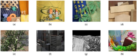
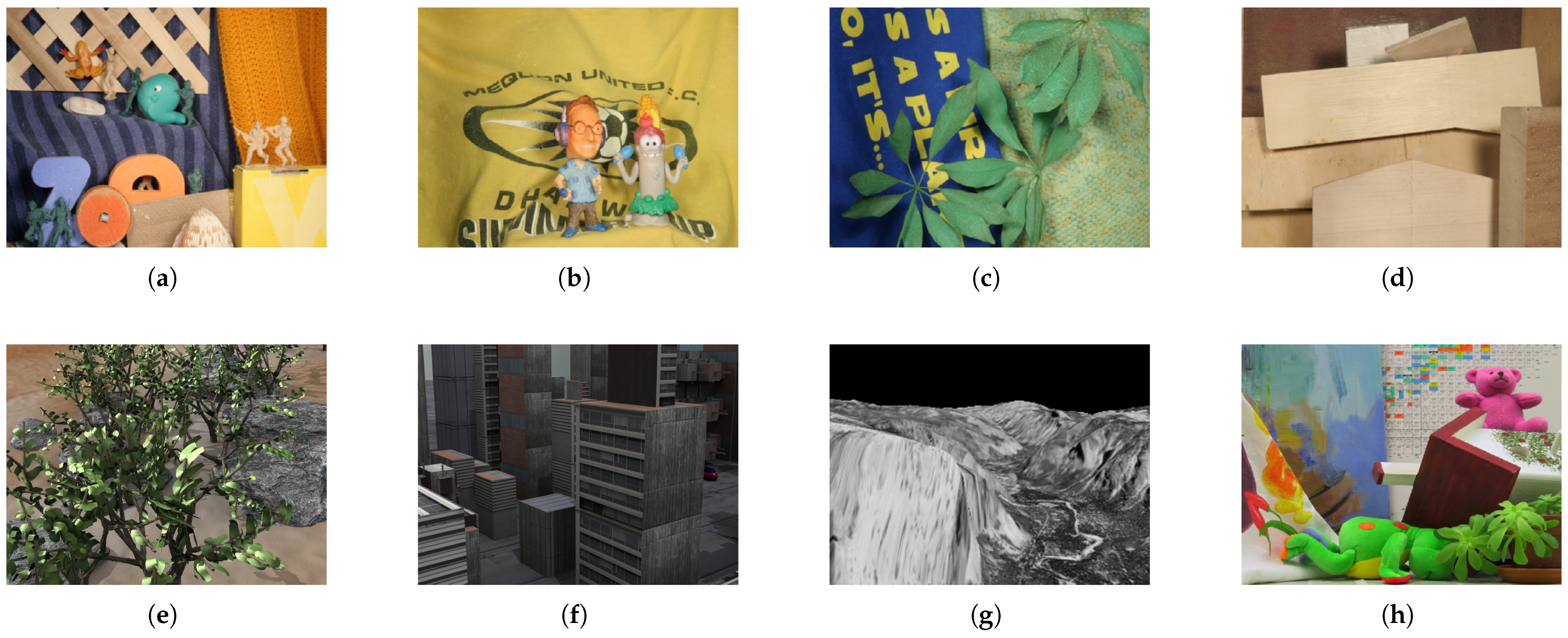
The selection of suitable datasets plays a fundamental role to evaluate the performance of optical flow models in image processing and computer vision. In this study, to demonstrate the efficiency of proposed non-linear fractional order variational model, eight widely recognized benchmark image sequences as shown in Figure 1 were selected from the Middlebury optical flow database (https://vision.middlebury.edu/flow/data/, accessed on 10 May 2026). The primary motivation for selecting these specific image sequences lies in their distinct and challenging motion characteristics; for Example, the image sequences such as Army, Mequon, Schefflera, and Wooden contain complex dynamic scenes with fine and hidden texture variations. In particular, the Army sequence is characterized by a complex motion field with sharp boundaries, the Mequon dataset contains texture-less regions and non-rigid motion combined with noticeable illumination variations, whereas the Schefflera sequence includes thin structures, shadowed regions, and foreground–background transitions with low intensity variations and the Wooden sequence exhibited low texture-regions, rigid motion and shadow effects [37]. Furthermore, to rigorously analyze the robustness of the proposed model, its performance was evaluated on synthetic image sequences, including the Grove, Urban, Yosemite, and Teddy image sequences. The Grove image dataset features a detailed tree scene with complex motion patterns and fine structures. The Urban image sequence contains sharp motion discontinuities and large displacements with independently moving vehicles. The Yosemite sequence is considered a standard benchmark for optical flow evaluation because it exhibits a complex and divergent flow fields [37].
Figure 1.
Sample reference images. First row: (a) Army, (b) Mequon, (c) Schefflera, and (d) Wooden. Second row: (e) Grove, (f) Urban, (g) Yosemite and (h) Teddy.
6.2. Performance Evaluation Metrics
In the literature, different quantitative metrics have been used to measure the efficiency of optical flow models. In this study, we focused on two widely accepted error metrics which are mainly suitable for evaluating the performance of the proposed model. Both error metrics are scalar quantities obtained by averaging over all pixels in the image domain. The corresponding error metrics are described as follows:
6.2.1. Average Angular Error ()
This error metric measures the mean angle difference between the estimated and ground-truth (original) flow [37,38]. The average angular error is defined as follows:
where and denote ground-truth and estimated flow vectors, respectively. The average angular error is effective in evaluating directional consistency [38].
6.2.2. Average Endpoint Error ()
The average end-point error is used to calculate the average Euclidean distance between the estimated and original flow fields. The average endpoint error is defined as follows:
a lower value of demonstrates a more accurate flow estimate. This metric is particularly advantageous in cases where is small [38].
6.3. Results and Discussion
In this section, we present a set of comprehensive numerical experiments, conducted to evaluate the performance of the proposed non-linear fractional order variational optical flow model, and the results were further validated through the comparison against existing well-established optical flow methods. All numerical experiments were performed using MATLAB R2024 on system equipped with an Intel(R) Core(TM) i3-8130U CPU @ 2.20GHz (manufactured by HP Inc., Palo Alto, CA, USA) and 8GB RAM. The experiments were performed using eight standard Benchmark datasets with various features as illustrated in Figure 1. For the experimental setup, we use these parameter values settings, where , and we compute the fractional-order gradients using the kernel size of the window . The qualitative results of the estimated flow are embodied by well-established Middlebury color maps, where the intensity of the color indicates the magnitude of motion and the color itself represents the direction of the pixel movement.
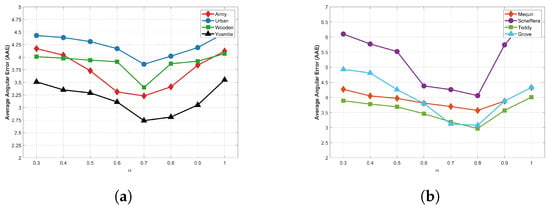
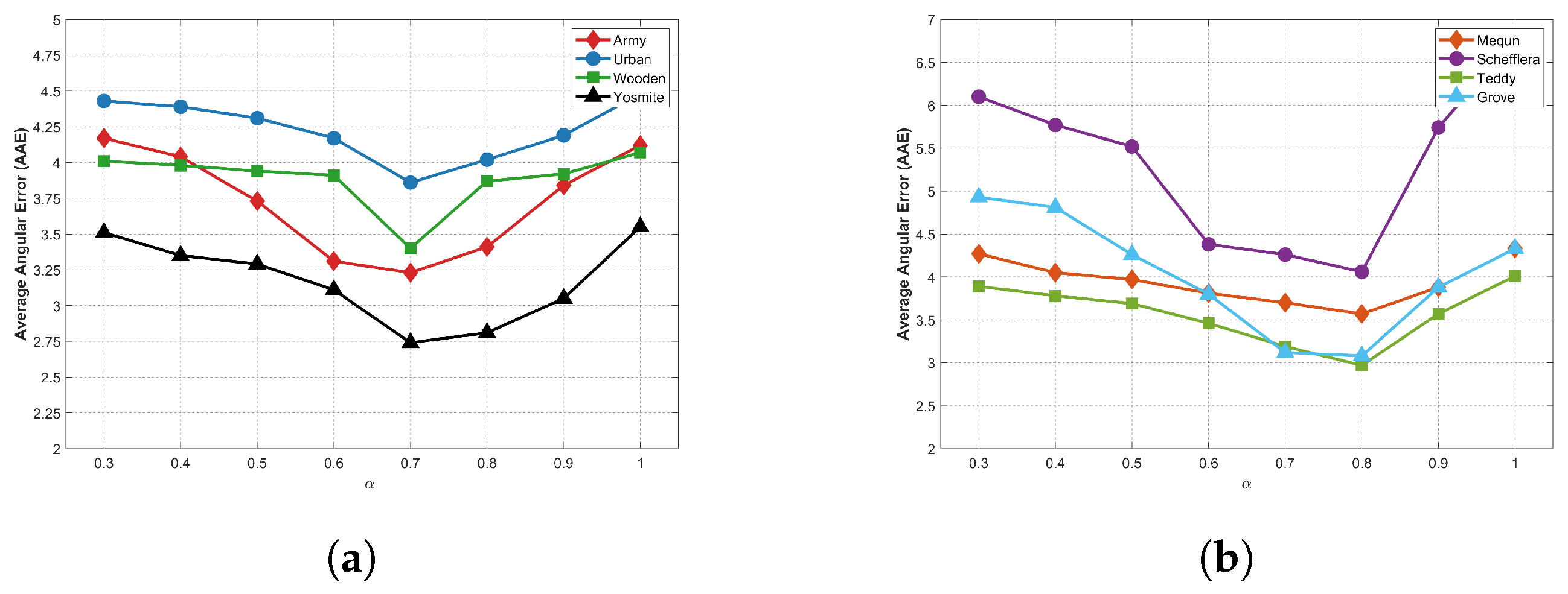
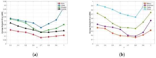
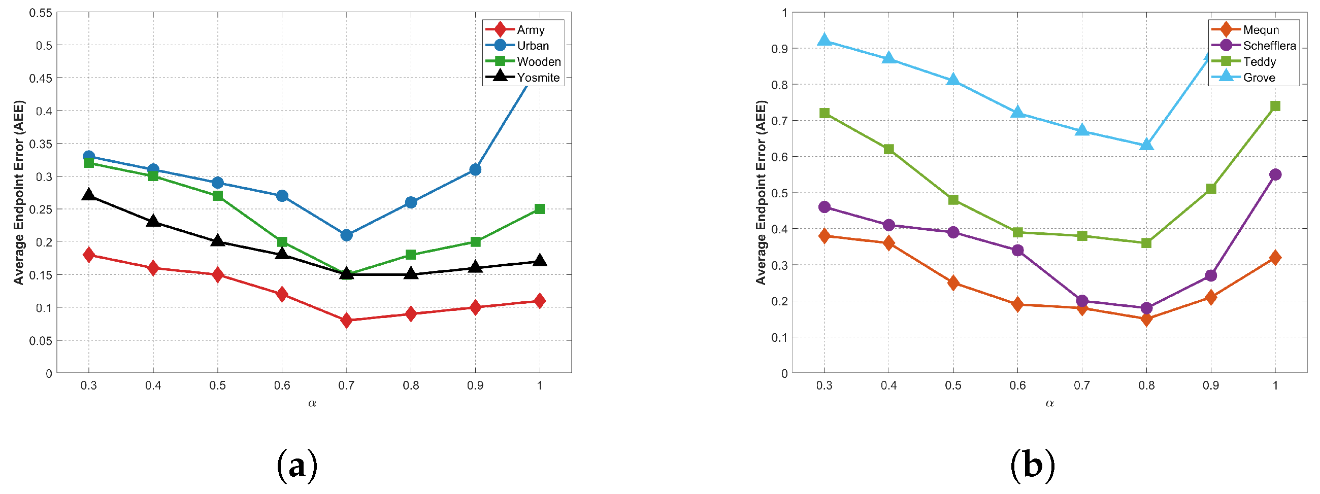
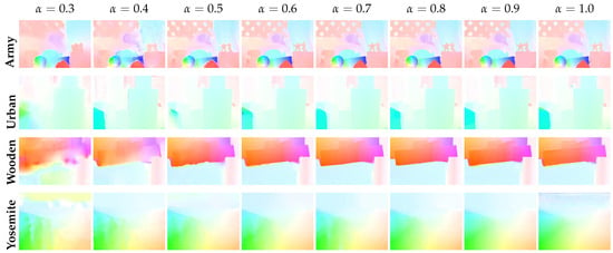
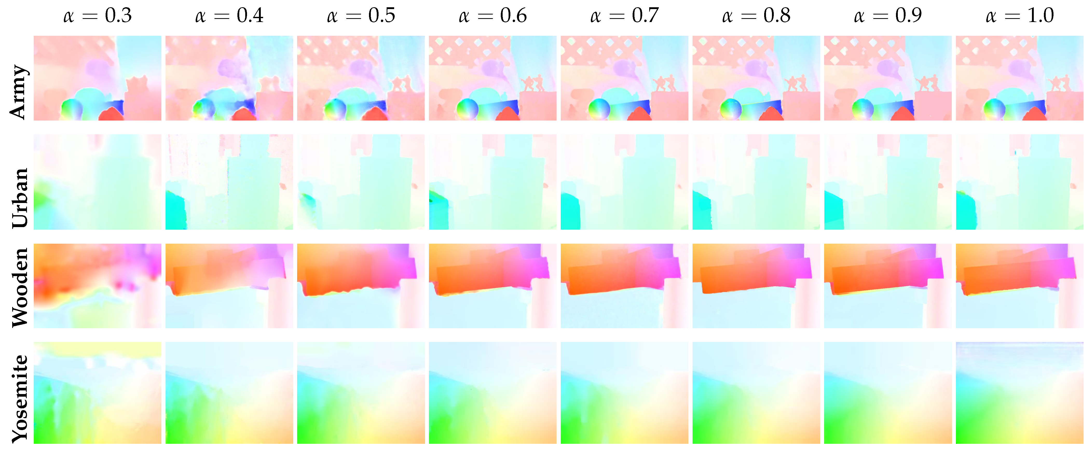
In the first experiment, we investigate the effect of the fractional-order parameter on the Army, Urban, Wooden, and Yosemite sequences within the interval . The corresponding quantitative results are presented in Figure 2a and Figure 3a, while the qualitative results are shown in Figure 4.
Figure 2.
Effect of fractional-order parameter (0.3–1.0) on average angular error for corresponding data sets: (a) Army, Urban, Wooden, Yosemite (b) Mequon, Schefflera, teddy, Grove.
Figure 3.
Effect of fractional-order parameter (0.3–1.0) on average end-point error for corresponding data sets: (a) Army, Urban, Wooden, Yosemite (b) Mequon, Schefflera, teddy, Grove.
Figure 4.
Estimated optical flow at different values of the fractional-order parameter for the Army (first row), Urban (second row), Wooden (third row), and Yosemite (fourth row) benchmark datasets.
From experimental evaluations it was observed that when the fractional-order parameter is constrained to lower values within , the proposed model exhibits strong regularization (i.e., over-smoothing). Consequently, this over-smoothing leads to degraded object boundaries, suppress fine texture details, and compromises the preservation of motion discontinuities as illustrated in Figure 4. Similarly, for , regularization becomes too weak, which leads to increased sensitivity to local intensity variations and noise amplifications, particularly in homogeneous regions. In contrast, the model uniformly produced lower angular error and the end-point error at . In particular, for the Army sequence with smaller values of the fractional-order parameter , the proposed model produces comparatively smoother flow fields. Whereas, it suffers from limitations in preserving fine motion discontinuities, as shown in Figure 4. However, best performance is observed at , where the proposed model balances global and local motion characteristics, producing significantly improved flow fields while successfully preserving sharp motion discontinuities. Conversely, when the increases within the interval , the model exhibits noise amplification in smooth regions and reduced robustness against illumination variations across the different objects.
Similarly, for the Urban sequence, the proposed model performed better at and yields minimum average angular error and end-point error values while maintaining the smoothing and edge preservation. At this optimal value, decreasing blurring effects are observed in both textured and uniform regions, such as buildings and roads as shown in Figure 4. On other hand, for the lower fractional orders (i.e., ), the proposed model induces strong regularization, which leads suppression in sharp motion gradients. At higher values of , the regularization term weakens considerably, introducing numerical instabilities and noise artifacts, particularly within low-texture sub-regions such as the sky and uniform wall boundaries. In the case of the Wooden sequence, the proposed model produces strong diffusion at lower fractional orders (i.e., ), leading to the degradation of subtle displacement variations across fine-scale structures. Whereas, at the proposed model ensures the preservation of texture continuity and suppress the noise in uniform regions. However, at higher fractional order values i.e., , less contribution of the regularization is observed, in result the model becomes more sensitive to noise and illumination variations in texture-less regions (Figure 4). Moreover, for the Yosemite sequence, setting the as , the model produce strong diffusion. Conversely, at higher values of fractional order parameter tend to introduce numerical artifacts and instability in regions, where motion field changes smoothly. Whereas, at the proposed model achieve the minimum average angular and average end-point error while accurately reconstructing the underlying vector field. In summary, the proposed model achieved best results for the Army, Urban, Wooden and Yosemite sequences at , with minimum average angular error and average end-point error.
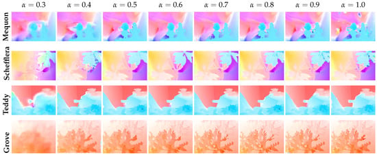
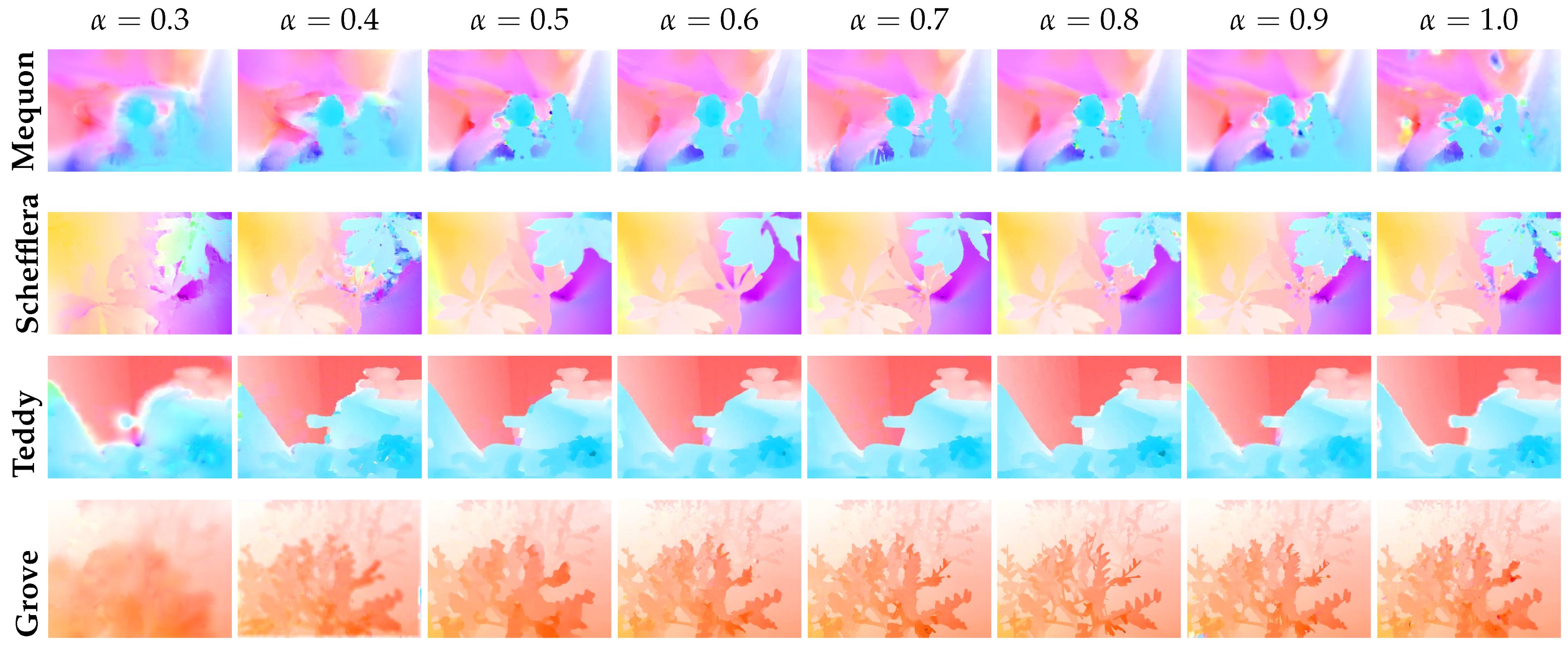
In second experiment, we evaluated the performance of the proposed model on the Mequon, Schefflera, Teddy, and Grove data sequences in a similar manner. From the results shown in Figure 5, it is observed that for a lower value of , the model produces strong regularization across all these sequences, which tends to over-suppress motion discontinuities. Consequently, fine motion structures are blurred and subtle texture details are lost. At these sequences achieved their ideal results by preserving sharp motion boundaries and capturing fine structural details. However, at regularization effect becomes less dominant, leading to increased sensitivity to local intensity variations and noise amplifications, particularly in the smooth regions. The proposed model attained the most favorable results for the Mequon, Schefflera, Teddy, and Grove sequences at with better smoothing and the motion boundaries preservation.
Figure 5.
Estimated optical flow at different values of the fractional-order parameter for Mequon (first row), Schefflera (second row), Teddy (third row), and Grove (fourth row) benchmark datasets.
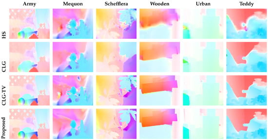
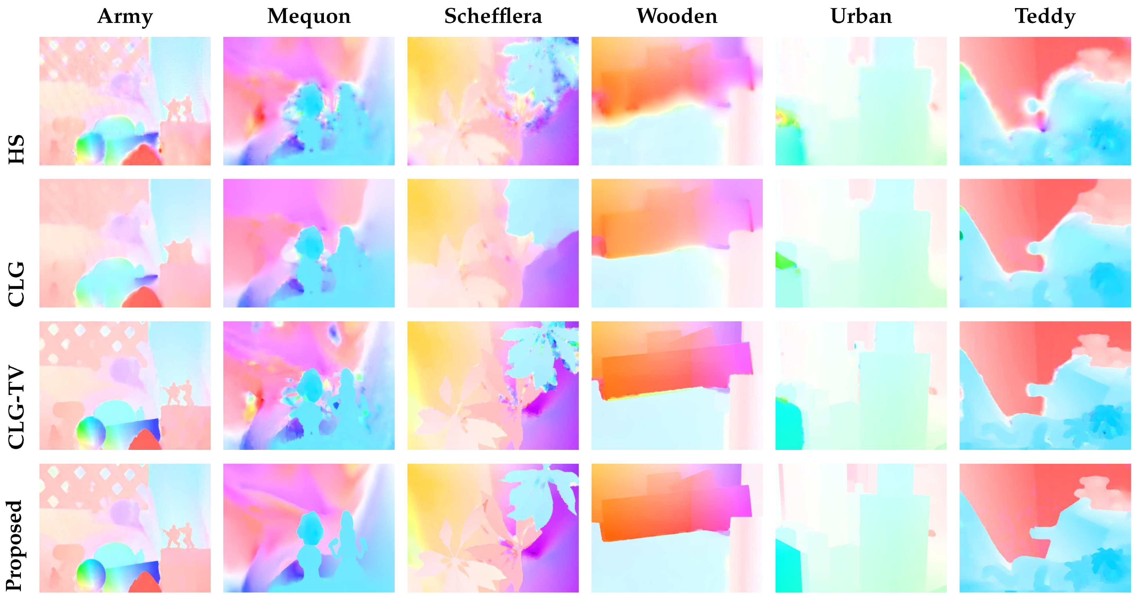
In third experiment, we conducted a comparative study against well-established optical flow methods, such as Horn and Schunck (HS) [18], combined local-global (CLG) [22] and combined local-global total variation (CLG-TV) [20] method to validate the performance of the proposed model. Across all sequences in the Figure 1, the proposed fractional-order model yields the lowest error (i.e., see in Table 1) of the four methods,and the margin is consistent rather than sequence specific, indicating better smoothing and edge preservation in complex texture patterns. Quantitative evaluation is performed using two widely accepted measures: Average Angular Error and Average Endpoint Error, as presented in Table 1. The experimental analysis presented in Figure 6 indicates that the HS model suffers from over-smoothing due to its global integer-order quadratic regularization, which blurs the motion boundaries and suppresses fine motion details. Although the CLG model improves local flow estimation owing to its local-global formulation, it still suffers from over-smoothing, particularly in textured regions, and suppresses weak gradients. Moreover, the CLG-TV model preserves motion boundaries more effectively; however, due to its integer-order total variation regularization formulation, it produces staircase artifacts in the smooth regions.
Table 1.
Comparative evaluation results of the proposed fractional order and conventional optical flow models (Horn-Schunck(HS) [18], Combined Local-global(CLG) [22], Combined Local-global Total Variation (CLG-TV) [20]) in terms of Average Angular Error and Average End-point Error for Middlebury sequences used in parameter optimization.
Figure 6.
Estimated optical flow fields obtained using different models. Columns: Army, Mequon, Schefflera, Wooden, Urban, and Teddy; Rows: Horn–Schunck (HS) [18], Combined Local–Global (CLG) [22], Combined Local–Global Total Variation (CLG-TV) [20], and the proposed model.
Particularly, in terms of average angular error, the proposed model ranges from –, against – for CLG-TV, – for CLG and – for HS; in terms of average end-point error it remains between pixels and pixels, whereas CLG-TV spans (0.11–0.92) pixels, CLG (0.28–1.54) pixels, and HS (0.22–1.51) pixels (Table 1). Relative to CLG-TV, the strongest conventional baseline, the reductions are to in AAE and to in AEE, with the largest end-point gains on Schefflera , Teddy and Urban . Notably, the relative ordering of HS and CLG is itself unstable: CLG is better in Grove vs. and Teddy ( vs. ), but very poor in Schefflera ( vs. ), Wooden ( vs. ) and Mequn ( vs. ) sequence. The fractional-order formulation removes this dependence, which suggests that tuning the differential order acts as a regulariser adapted to the local texture and edge content of each sequence rather than favoring one particular smoothing scheme.
These findings are consistent with, and extend, earlier benchmark evidence, where [37] reported that the combined local-global method exhibited superior performance over their preliminary Middlebury study, with average end-point errors below pixels in the Yosemite, Army, Mequon and Wooden sequence, and identified Grove, Teddy, Urban and Schefflera as the challenging sequences due to large motions and strong flow discontinuities. These conventional methods reflect this exact pattern, such as the highest value for corresponds to Teddy (), Urban () and Grove () for the HS model, Urban (), Teddy () and Grove () for the CLG method, and Grove (), Teddy () and Schefflera () for the CLG-TV framework. Significantly, the proposed non-linear fractional-order method demonstrates its substantial performance enhancements precisely on these challenging sequences.
7. Conclusions
Keeping in view the different shortcomings in conventional optical flow models, we introduced a non-linear fractional-order variational model for optical flow estimation in this paper. The proposed model generalizes classical methods by introducing fractional-order gradients. Particularly, it integrates a non-linear fractional order total variation regularizer with the robust fidelity term of Lucas-Kanade model. The results on the existence of a minimizer for the proposed model are established as an additional contribution, offering valuable insights to the readers in this research area. These existence results allow the application of direct methods from the calculus of variations to find the optimizer for the proposed model. Following this optimization process, the discretization of the fractional-order gradients was performed using the Grunwald-Letnikov discretization operator. The obtained non-linear system was then transformed into a linear system via the lagged diffusivity fixed-point linearization technique, and then the optical flow field was computed efficiently using the Gauss-Siedel iterative method. The simulation results are presented in Figure 4 and Figure 5, respectively. The performance of the proposed model was examined using Middleburry benchmark standard data sets (different image sequences), as shown in Figure 1. Experimental evaluation of these standard Middleburry benchmark sequences shows that our method produced a dense flow field and achieved a significant improvement in the preservation of motion discontinuities at different values of the fractional order derivative parameter . The optimal value of was determined using the minimum error measures as illustrated in Figure 2 and Figure 3. Furthermore, the comparative results illustrated in Figure 6 and Table 1 confirm that, for the evaluated benchmark datasets, the proposed model achieved significantly better results compared to conventional optical flow variational models in terms of robustness and preservation of motion discontinuities. Although the empirical results demonstrate the effectiveness of the model in handling textured regions and preserving discontinuities across the evaluated benchmark sequences, these performance gains remain specific to the unique motion-texture characteristics of the tested datasets rather than acting as universal guaranties. The theoretical formulation ensures a mathematically sound integration of fractional-order derivatives providing a generalized framework that inherently accounts for non-local variations. However, establishing good performance that makes it possible to apply the method to other unconstrained real-world video scenarios is beyond the scope of the current evaluation at this stage.
In future work, different types of fractional-order diffusion penalties can be added along with a suitable choice of data term for more efficient results. In addition, the applications of the proposed model can be extended using machine-learning techniques. Another possible extension is to design a locally adaptive strategy that can be developed by replacing the fixed regularization parameter with an adaptive control function that can automatically balance smoothness and moving discontinuities. Furthermore, the proposed non-linear fractional-order model can be applied to other image processing applications, including image denoising and image segmentation, where discontinuity preservation is significantly important.
Author Contributions
Conceptualization, I.A.A. and K.B.A.; methodology, I.A.A., K.B.A. and M.B.A.; formal analysis, I.A.A. and M.B.A.; investigation, I.A.A., M.B.A. and G.Y.M.; writing—original draft preparation, I.A.A.; writing—review and editing, K.B.A., M.B.A. and G.Y.M.; supervision, K.B.A. All authors have read and agreed to the published version of the manuscript.
Funding
This research received no external funding.
Data Availability Statement
No new data were created or analyzed in this study. Data sharing is not applicable to this article.
Acknowledgments
The authors declare they have not used Artificial Intelligence (AI) tools in the creation of this article.
Conflicts of Interest
The authors declare no conflict of interest.
References
- Shah, S.T.H.; Xuezhi, X. Traditional and modern strategies for optical flow: An investigation. SN Appl. Sci. 2021, 3, 289. [Google Scholar] [CrossRef] [Scilit]
- Wang, Y.; Wang, W.; Li, Y.; Guo, J.; Xu, Y.; Ma, J.; Ling, Y.; Fu, Y.; Jia, Y. Research on traditional and deep learning strategies based on optical flow estimation—A review. J. King Saud Univ. Comput. Inf. Sci. 2024, 36, 102029. [Google Scholar] [CrossRef] [Scilit]
- Elasri, A.; Cherroun, L.; Nadour, M. Robotic visual-based navigation structures using Lucas-Kanade and Horn-Schunck algorithms of optical flow. Iran. J. Sci. Technol. Trans. Electr. Eng. 2024, 48, 1149–1172. [Google Scholar] [CrossRef] [Scilit]
- Alfarano, A.; Maiano, L.; Papa, L.; Amerini, I. Estimating optical flow: A comprehensive review of the state of the art. Comput. Vis. Image Underst. 2024, 244, 104160. [Google Scholar] [CrossRef] [Scilit]
- Lavín-Delgado, J.E.; Gómez-Aguilar, J.F.; Pérez-Careta, E.; Olivares-Peregrino, V.H.; Torres-Jiménez, J. On the estimation of optical flow: A novel robust estimation based in fractional derivatives with kernel exponential. Int. J. Model. Simul. Sci. Comput. 2025, 16, 25500539. [Google Scholar] [CrossRef] [Scilit]
- Barron, J.L.; Fleet, D.J.; Beauchemin, S.S. Performance of optical flow techniques. Int. J. Comput. Vis. 1994, 12, 43–77. [Google Scholar] [CrossRef] [Scilit]
- Zhai, M.; Xiang, X.; Lv, N.; Kong, X. Optical flow and scene flow estimation: A survey. Pattern Recognit. 2021, 114, 107861. [Google Scholar] [CrossRef] [Scilit]
- Miller, K.S. An Introduction to the Fractional Calculus and Fractional Differential Equations; John Wiley & Sons: New York, NY, USA, 1993. Available online: https://lccn.loc.gov/93009500 (accessed on 20 May 2026).
- Khan, M.; Kumar, P. A nonlinear modeling of fractional order based variational model in optical flow estimation. Optik 2022, 261, 169136. [Google Scholar] [CrossRef] [Scilit]
- Singh, B.; Kumar, P. Optical flow with non-local weight and fractional order regularization: A variational model with superpixel algorithm for various application oriented spectrum. Arab. J. Sci. Eng. 2024, 50, 15297–15327. [Google Scholar] [CrossRef] [Scilit]
- Chen, D.; Sheng, H.; Chen, Y.; Xue, D. Fractional-order variational optical flow model for motion estimation. Philos. Trans. R. Soc. A 2013, 371, 20120148. [Google Scholar] [CrossRef] [Scilit]
- Kumar, P.; Kumar, S.; Raman, B. A fractional order variational model for the robust estimation of optical flow from image sequences. Optik 2016, 127, 8710–8727. [Google Scholar] [CrossRef] [Scilit]
- Saleem, S.; Ahmad, S.; Kim, J. Total fractional-order variation-based constraint image deblurring problem. Mathematics 2023, 11, 2869. [Google Scholar] [CrossRef] [Scilit]
- Charkaoui, A.; Ben-loghfyry, A. Anisotropic equation based on fractional diffusion tensor for image noise removal. Math. Methods Appl. Sci. 2024, 47, 9600–9620. [Google Scholar] [CrossRef] [Scilit]
- Diwakar, M.; Singh, P.; Garg, D. Edge-guided filtering based CT image denoising using fractional order total variation. Biomed. Signal Process. Control 2024, 92, 106072. [Google Scholar] [CrossRef] [Scilit]
- Singh, B.; Kumar, P. A non-local weighted fractional order variational model for motion estimation. Procedia Comput. Sci. 2025, 260, 865–872. [Google Scholar] [CrossRef] [Scilit]
- Bertero, M.; Poggio, T.A.; Torre, V. Ill-posed problems in early vision. Proc. IEEE 1988, 76, 869–889. [Google Scholar] [CrossRef] [Scilit]
- Horn, B.K.P.; Schunck, B.G. Determining optical flow. Artif. Intell. 1981, 17, 185–203. [Google Scholar] [CrossRef] [Scilit]
- Lucas, B.D.; Kanade, T. An iterative image registration technique with an application to stereo vision. In Proceedings of the 7th International Joint Conference on Artificial Intelligence (IJCAI’81), Vancouver, BC, Canada, 24–28 August 1981; Volume 2, pp. 674–679. Available online: https://hal.science/hal-03697340/ (accessed on 23 August 2026).
- Drulea, M.; Nedevschi, S. Total variation regularization of local-global optical flow. In Proceedings of the 2011 14th International IEEE Conference on Intelligent Transportation Systems (ITSC), Washington, DC, USA, 5–7 October 2011; pp. 318–323. [Google Scholar] [CrossRef] [Scilit]
- Doshi, H.; Kiran, N.U. A variational optical flow model for accurate motion estimation from rotational image sequences. SN Comput. Sci. 2024, 5, 359. [Google Scholar] [CrossRef] [Scilit]
- Bruhn, A.; Weickert, J.; Schnörr, C. Lucas/Kanade meets Horn/Schunck: Combining local and global optic flow methods. Int. J. Comput. Vis. 2005, 61, 211–231. [Google Scholar] [CrossRef] [Scilit]
- Black, M.J.; Anandan, P. The robust estimation of multiple motions: Parametric and piecewise-smooth flow fields. Comput. Vis. Image Underst. 1996, 63, 75–104. [Google Scholar] [CrossRef] [Scilit]
- Brox, T.; Bruhn, A.; Papenberg, N.; Weickert, J. High accuracy optical flow estimation based on a theory for warping. In Computer Vision—ECCV 2004: 8th European Conference on Computer Vision; Springer: Berlin/Heidelberg, Germany, 2004; pp. 25–36. [Google Scholar] [CrossRef] [Scilit]
- Weickert, J.; Schnörr, C. Variational optic flow computation with a spatio-temporal smoothness constraint. J. Math. Imaging Vis. 2001, 14, 245–255. [Google Scholar] [CrossRef] [Scilit]
- Nagel, H.-H.; Enkelmann, W. An investigation of smoothness constraints for the estimation of displacement vector fields from image sequences. IEEE Trans. Pattern Anal. Mach. Intell. 1986, PAMI-8, 565–593. [Google Scholar] [CrossRef] [Scilit]
- Rudin, L.I.; Osher, S.; Fatemi, E. Nonlinear total variation based noise removal algorithms. Physica D. Nonlinear Phenom. 1992, 60, 259–268. [Google Scholar] [CrossRef] [Scilit]
- Pérez, J.S.; Meinhardt-Llopis, E.; Facciolo, G. TV-L1 optical flow estimation. Image Process. Line 2013, 3, 137–150. [Google Scholar] [CrossRef] [Scilit]
- Zach, C.; Pock, T.; Bischof, H. A duality based approach for realtime TV-L1 optical flow. In Pattern Recognition: 29th DAGM Symposium; Springer: Berlin/Heidelberg, Germany, 2007; pp. 214–223. [Google Scholar] [CrossRef] [Scilit]
- Arain, M.B.; Amur, K.B.; Katbar, N.M.; Tolasa, F.T. Adaptive regularization for combined linear and nonlinear color image diffusion with normalized data. Signal Image Video Process. 2025, 19, 601. [Google Scholar] [CrossRef] [Scilit]
- Yang, Q.; Chen, D.; Zhao, T.; Chen, Y. Fractional calculus in image processing: A review. Fract. Calc. Appl. Anal. 2016, 19, 1222–1249. [Google Scholar] [CrossRef] [Scilit]
- Schönberger, H. Extending linear growth functionals to functions of bounded fractional variation. Proc. R. Soc. Edinb. Sect. A Math. 2024, 154, 304–327. [Google Scholar] [CrossRef] [Scilit]
- Gelfand, I.M.; Silverman, R.A. Calculus of Variations; Courier Corporation: Chelmsford, MA, USA, 2000. [Google Scholar]
- Aubert, G.; Kornprobst, P. Mathematical Problems in Image Processing: Partial Differential Equations and the Calculus of Variations; Springer: New York, NY, USA, 2006; Volume 147. [Google Scholar] [CrossRef] [Scilit]
- Vogel, C.R.; Oman, M.E. Iterative methods for total variation denoising. SIAM J. Sci. Comput. 1996, 17, 227–238. [Google Scholar] [CrossRef] [Scilit]
- Saad, Y. Iterative Methods for Sparse Linear Systems; Society for Industrial and Applied Mathematics (SIAM): Philadelphia, PA, USA, 2003. [Google Scholar]
- Baker, S.; Scharstein, D.; Lewis, J.P.; Roth, S.; Black, M.J.; Szeliski, R. A database and evaluation methodology for optical flow. Int. J. Comput. Vis. 2011, 92, 1–31. [Google Scholar] [CrossRef] [Scilit]
- Fleet, D.J.; Jepson, A.D. Computation of component image velocity from local phase information. Int. J. Comput. Vis. 1990, 5, 77–104. [Google Scholar] [CrossRef] [Scilit]

Disclaimer/Publisher’s Note: The statements, opinions and data contained in all publications are solely those of the individual author(s) and contributor(s) and not of MDPI and/or the editor(s). MDPI and/or the editor(s) disclaim responsibility for any injury to people or property resulting from any ideas, methods, instructions or products referred to in the content. |
© 2026 by the authors. Licensee MDPI, Basel, Switzerland. This article is an open access article distributed under the terms and conditions of the Creative Commons Attribution (CC BY) license.