


Abstract
We study regular Sturm–Liouville problems on whose coefficients are generated by smooth activation functions with positive offsets, so that for every parameter vector . The classical conservative three-point scheme yields a symmetric-definite tridiagonal pencil with simple eigenvalues for every . Besides verifying second-order accuracy, we contribute: exact derivatives of every discrete eigenvalue with respect to every activation parameter at cost, converging at to the continuous sensitivities; mesh-independent min–max bounds on eigenvalue shifts under coefficient perturbations; the generalized locally Toeplitz symbol of the discretization; and an identifiability analysis of calibration. With correctly computed orders, eigenvalue errors converge at rates 1.991–2.004 on four benchmarks, including one with closed-form eigenpairs for ; weighted orthogonality holds to the level of rounding error; a half-cell treatment gives second order for Robin conditions. Sampled coefficients alone determine the six activation parameters; eigenvalues add information when coefficient data are partial (with the potential unobserved, two to four eigenvalues recover all parameters in 20 of 20 starts), and eigenvalues alone do not identify them. Comparison with Chebyshev collocation and Pyslise (MATSLISE) shows that the scheme is less accurate for fixed smooth coefficients; its value lies in structure preservation and cheap exact gradients.
Keywords:
Sturm–Liouville eigenvalue problem; activation-function coefficients; conservative finite differences; second-order convergence; eigenvalue sensitivity; min–max perturbation bounds; generalized locally Toeplitz sequences; parameter identification; identifiability MSC:
34L16 (Primary); 65L15; 65L12; 34B24; 65F15; 34A55
1. Introduction
Sturm–Liouville theory links differential equations, spectral analysis, numerical approximation, and applied modeling. A second-order operator with sufficiently regular coefficients (for instance , with ) and separated self-adjoint boundary conditions has a real, simple, discrete spectrum and a complete set of eigenfunctions that are orthogonal in a weighted inner product [1,2]. These properties underpin separation of variables, modal analysis, vibration and wave problems [3], quantum mechanics [4], spectral filtering [5], and mathematical finance, where Sturm–Liouville theory underlies the recovery of physical from risk-neutral probabilities [6].
The analytical theory continues to be refined: De Oliveira and Maiorino [7] give a modern applied exposition, De Gregorio et al. [8] revisit classical results for a non-constant weight, including the large- trigonometric behavior of solutions, completeness via the Phragmén–Lindelöf theorem and uniform convergence of eigenfunction expansions, Derkach and Malamud [9] treat Sturm–Liouville operators within the extension theory of symmetric operators, and Karjanto and Sadhani [10] discuss the reduction of general problems to canonical (Liouville) form. Discrete analogues have been studied by Migda et al. [11], optimization problems on the nodes of Sturm–Liouville operators by Chu et al. [12], and problems with discontinuous nonlinearities, distributional, or indefinite weights and fractional derivatives in [13,14,15,16].
The numerical solution of Sturm–Liouville problems is a mature field. The accuracy of finite-difference eigenvalue approximations was analyzed by Keller [17]; the monograph of Pryce [18] surveys finite-difference, shooting, and coefficient-approximation methods. Paine, de Hoog, and Anderssen [19] showed that the finite-difference error of the -th eigenvalue grows like and derived an asymptotic correction that removes this growth. Robust general-purpose codes are available: SLEIGN2 [20] and SLEDGE [21] (Prüfer-type and coefficient-approximation methods), and MATSLISE [22] together with its Python successor Pyslise [23] (constant-perturbation methods). Spectral collocation [24], sinc-Galerkin [4], boundary-shape-function [25], and matrix-eigenvalue polynomial [26] methods, as well as the earlier procedure of Mikhailov and Vulchanov [27], complete the picture. A complementary, global viewpoint is provided by the theory of (generalized) locally Toeplitz sequences [28,29,30]: the matrices produced by the conservative three-point scheme are exactly of the type analyzed in Section 10.5 of the book by Garoni and Serra-Capizzano [30], and their spectra are asymptotically described by a symbol. Inverse Sturm–Liouville problems have a long history, from Borg’s uniqueness theorem [31] to reconstruction algorithms [32,33,34].
Learning-based approaches have recently been proposed: Zhang et al. [35] compute eigenpairs with deep networks, and Vigouroux et al. [36] use Sturm–Liouville problems with learnable coefficients to build orthogonal bases for regularization. In these approaches, the coefficient functions are typically flexible maps for which positivity of and , and hence, self-adjointness and orthogonality, must be enforced explicitly.
Scope and contributions. This paper does not propose a new discretization. We use the classical conservative three-point scheme, whose second-order accuracy and preservation of self-adjointness are well-known [17,18], and we make no claim of higher accuracy than spectral or Prüfer-based solvers (Section 4.5 shows the opposite for fixed smooth coefficients). The convergence and orthogonality results for activation-generated coefficients are therefore expected, since such coefficients are smooth and uniformly positive; we report them as a verification of the implementation. The contributions that are specific to activation-parameterized coefficients are:
(C1) an admissibility construction in which every parameter vector defines a regular problem and an unreduced symmetric-definite tridiagonal pencil, so that all discrete eigenvalues are simple for every (Proposition 1, Lemma 1);
(C2) closed-form exact derivatives of the discrete eigenvalues with respect to the activation parameters, together with their continuous counterparts and an convergence result verified numerically (Proposition 2);
(C3) mesh-independent two-sided eigenvalue bounds under coefficient perturbations, derived from the min–max principle and compared with first-order predictions (Theorem 3);
(C4) the GLT symbol of the activation-parameterized discretization, which describes the whole discrete spectrum and quantifies which part of it is accurate (Proposition 3);
(C5) a calibration study with exact gradients, including an identifiability analysis showing which combinations of eigenvalue and coefficient data determine the six activation parameters: eigenvalues alone do not, complete coefficient samples do without eigenvalues, and eigenvalues supply the missing information when the coefficient data are partial;
(C6) a complete specification of all computational settings (meshes, coefficients, perturbation profiles, objective weights, and optimizer tolerances), so that every number in the paper can be reproduced from the text.
We regard the activation parameterization as a constrained, low-dimensional parameter-identification model; it is not a neural network, and the paper does not perform machine learning. The connection to learning-based methods is that the same coefficient generators and exact gradients can be embedded in larger differentiable pipelines; this is discussed as an outlook in Section 5. Table 1 positions the study.
Table 1.
Literature synthesis and position of the present study.
2. The Mathematical Model
Let . Following the standard formulation of regular Sturm–Liouville problems [1,2], the activation-parameterized problem is
where is the eigenvalue, the eigenfunction, and , , are the diffusion, potential, and weight coefficients. The subscript denotes dependence on a finite parameter vector (scales, slopes and offsets of the activation maps). Positivity is imposed by construction:
with constants and , and real and continuous. The functions and are compositions of affine maps or with nonnegative activations (softplus, , sigmoid). Throughout, and denote the lower bounds of and on . The separated boundary conditions are
The analysis of Section 3 covers general separated conditions where stated; the discretization, convergence theorem, and benchmarks B1–B4 use Dirichlet conditions , and the Robin case is treated separately in Section 3.3 and Section 4.4. The weighted space carries the inner product
and the operator form of (1) is with . Integration by parts with (4)–(5) gives the bilinear form
where a boundary term is present only when (respectively, ). The form domain is for Dirichlet conditions at both ends, for Robin or Neumann conditions at both ends, and the corresponding mixed space otherwise. The problem is linear in for fixed ; the dependence on is nonlinear and is the subject of Section 3.4 and Section 4.8. Table 2 lists the assumptions under which each result holds.
Table 2.
Notation and the assumptions used by each result.
Admissible Activation Coefficients
Proposition 1 (admissibility).
Let and be defined by (2)–(3) with , finite compositions of affine maps, and the activations softplus, , or sigmoid, and let be a finite combination of such maps. Then, for every finite the coefficients belong to , , , and (1), with (4)–(5) is a regular Sturm–Liouville problem satisfying all assumptions of Table 2.
Proof.
Softplus, , and the sigmoid are real-analytic on , and softplus, , and the sigmoid are nonnegative. Compositions and products of real-analytic functions with affine maps and are real-analytic on , so and , . Regularity of the problem follows from [1] (Chapter 4). □
Admissibility is preserved along any optimization path: every iterate produced by an optimizer defines an admissible problem, so no projection or penalty is required. Table 3 summarises the activation choices.
Table 3.
Activation choices and their mathematical consequences.
3. Discretization and Analysis
3.1. Conservative Three-Point Scheme
We use the classical conservative (flux-form) three-point scheme [17,18]; its matrices are those analyzed in [30] (Section 10.5). Let , for , and . Write , , and . The flux term at an interior node is approximated by
With Dirichlet conditions , this yields the symmetric tridiagonal matrix and the diagonal matrix ,
and the generalized eigenvalue problem
Eigenvectors are normalized in the discrete weighted norm
and their sign is fixed by . Because is diagonal and positive, (11) is equivalent to the standard symmetric tridiagonal problem for , with . All computations use this reduction and the LAPACK tridiagonal eigensolver, at cost operations per eigenvalue and per eigenvector. Here, is the bisection tolerance relative to the width of the spectral interval: each bisection step evaluates a Sturm sequence in operations, and about steps are needed; each eigenvector is then obtained by inverse iteration with a bounded number of steps.
Lemma 1.
For every admissible and every , is an unreduced symmetric tridiagonal matrix. Consequently, the eigenvalues of (11) are real and simple, , and the eigenvectors are -orthogonal.
Proof.
The off-diagonal entries of are because . An unreduced symmetric tridiagonal matrix has simple eigenvalues, since for any , the first columns of are linearly independent. Orthogonality of eigenvectors of gives for . □
Lemma 1 is the discrete analogue of the simplicity of Sturm–Liouville eigenvalues and guarantees that the eigenvalue derivatives of Section 3.4 exist for every . Algorithm 1 summarises the solver.
| Algorithm 1. Activation-parameterized finite-difference eigensolver |
| Input: parameter vector |
| ; activation generators for , , ; number of interior nodes ; number of modes . |
| Output: eigenvalues and eigenvectors with , . |
| 1: Set , , . |
| 2: Evaluate () and , (); by Proposition 1, and . |
| 3: Form the diagonal and off-diagonal of from (9)–(10). |
| 4: Compute the smallest eigenpairs of with a symmetric tridiagonal eigensolver. |
| 5: Set , rescale to and fix the sign by . |
| 6: Return . |
3.2. Well-Posedness
Theorem 1.
Suppose , , , , and let the boundary conditions (4)–(5) hold. Then the eigenvalues of (1) are real and simple and form a sequence . The eigenfunctions form an orthogonal basis of , the -th eigenfunction has exactly zeros in , and each eigenfunction is unique once it is normalized in and its sign is fixed.
Proof.
This is the classical theorem for regular problems [1] (Theorems 4.3.1 and 4.6.2), [2]; we indicate the structure. The form (7) is symmetric, bounded on the form domain and, since and and the boundary terms are bounded (the latter by the trace inequality ), satisfies for some constants and . Hence, the operator associated with in is self-adjoint and bounded below, and because the embedding of into is compact on a bounded interval, its resolvent is compact. The spectral theorem gives a real discrete spectrum accumulating only at and an orthogonal eigenbasis. Simplicity holds because two eigenfunctions with the same eigenvalue satisfy the same separated condition at , so their Wronskian vanishes there and hence everywhere. The oscillation property is Sturm’s theorem. Since each eigenspace is one-dimensional, normalization and a sign convention determine the eigenfunction. □
3.3. Convergence
Theorem 2.
Let Dirichlet conditions hold, , , , , and fix . Let . There are and , depending on , the coefficient bounds and but not on , such that for the -th eigenpair of satisfies
where is restricted to the grid and both and are normalized by (12) with the same sign convention.
Proof.
The result is classical [17,18]; we give a short self-contained argument. Since by the regularity assumptions, Taylor expansion of (8) about gives the residual with . Put and . For a symmetric matrix, every and satisfy . With , the right-hand side is , where is a lower bound for the discrete root-mean-square of . Keller’s theorem [17] ensures for each fixed , so for , the eigenvalue of closest to is , which proves (13). For (14), the Davis–Kahan bound gives , and the denominator exceeds for ; translating back with and the normalization (12) gives (14). □
Remark 1.
(i) By Theorem 1, all eigenvalues of a regular problem with separated conditions are simple, so the assumption always holds. What matters in practice is its size: under strong coefficient contrast (for instance a weight concentrated in two separated subintervals), consecutive eigenvalues can be very close, is small, and the constant in (14) is large; for periodic conditions, eigenvalues can be genuinely double and a subspace estimate is needed. (ii) The constant in (13) grows with the mode number: for , the exact discrete eigenvalues give , and Paine, de Hoog, and Anderssen [19] show that growth is generic. For benchmark B4, we measure for , consistent with this growth (ratio 305 between and , compared with ).
Robin conditions. For at the value is unknown. Integrating (1) over the half cell and using gives the boundary row
which, together with the interior rows (9), yields a symmetric matrix and the diagonal mass matrix . The pencil remains symmetric definite, and Lemma 1 still applies. Section 4.4 confirms second-order convergence numerically; a proof follows the same lines as Theorem 2 with a boundary consistency term of order on a half cell weighted by [18], but we do not pursue it here.
3.4. Eigenvalue Sensitivity with Respect to Activation Parameters
Let be in with values in . Since every eigenvalue is simple (Theorem 1, Lemma 1), analytic perturbation theory [37] (Chapter VII) shows that and are in .
Proposition 2 (eigensensitivity) .
Let be the eigenfunction of (1) with Dirichlet conditions normalized by . Then
For the discrete problem (11) with normalized by (12), and ,
Proof.
Differentiate with respect to and multiply on the left by . By symmetry, , so the terms containing cancel and the first identity in (17) follows [38]. The quadratic form equals by summation by parts, and by (12), which gives the second identity. The continuous Formula (16) is obtained in the same way from the weak form (7) (Hellmann–Feynman identity), using and . □
Formula (17) is the exact derivative of the computed eigenvalue, not an approximation, and is the discrete quadrature of (16). Once is available, it costs operations per parameter, and no derivative of the eigenvector is needed. For the six-parameter family of Section 4.8, the derivatives , , and are explicit; for example, , where is the logistic sigmoid. Numerically, (17) agrees with central differences of step to within a relative difference of (the level of the finite-difference truncation error), and the discrete derivatives converge to the continuous ones with observed order 2.008, 2.002, 2.002, 2.004 (Section 4.8).
3.5. Perturbation Bounds
The following result quantifies how far the eigenvalues can move under bounded coefficient perturbations. It uses only the min–max principle [39] and holds verbatim for the continuous eigenvalues and for the discrete eigenvalues of (11) at every mesh size.
Theorem 3.
Let Dirichlet conditions hold and . Consider perturbed coefficients , and with measurable , , satisfying , and . Then, for every , with ,
where the lower bound requires . The same inequalities hold for and for every , when , , are replaced by their grid values. The upper bound holds without when only is perturbed (), and in that case .
Proof.
Write with and . For , , and . Since , , so the perturbed Rayleigh quotient satisfies with the increasing function . The min–max characterisation over subspaces (the same form domain for both problems) then gives . The lower bound is analogous with , which is valid as a lower bound for whenever the numerator is nonnegative. In the discrete case and , so the same steps apply with the Courant–Fischer theorem for the pencil . □
Theorem 3 also explains the signs observed in experiments: is non-decreasing in and and non-increasing in . A perturbation profile that changes sign, such as , can therefore move different eigenvalues in different directions; only the bounds (18) constrain the shift. To first order, the shift is given by (17).
3.6. Spectral Distribution: The GLT Viewpoint
Theorem 2 concerns a fixed mode as . The theory of generalized locally Toeplitz (GLT) sequences [28,29,30] describes instead the asymptotic distribution of all discrete eigenvalues. The matrices are exactly the finite-difference matrices treated in [30] (Section 10.5).
Proposition 3.
Let , be continuous and positive and bounded on . Then is a GLT sequence with symbol , has symbol , and the eigenvalues of (equivalently of the symmetric matrix ) are distributed as
that is, for every continuous with compact support.
Proof.
The symbol of the finite-difference matrices of with continuous is derived in [30] (Section 10.5); has spectral norm and is therefore zero-distributed, which does not change the symbol. Diagonal sampling matrices of a continuous function form a GLT sequence with symbol , and GLT sequences form a -algebra [30] (Chapters 8–9). Writing with continuous shows that is GLT with symbol . Since is symmetric, its eigenvalues, which are those of , are distributed as [30] (Chapters 8–9) [28,29]. □
Remark 2.
The hypotheses of Proposition 3 are stronger than the GLT theory requires. The symbol and the distribution result remain valid when , and are not smooth, and also when or has isolated zeros [28,29,30]. In the latter case the symbol is unbounded, but (19) still describes the asymptotic distribution of the discrete eigenvalues, even though individual discrete eigenvalues may then differ considerably from the eigenvalues of the continuous operator. We state Proposition 3 under the assumptions used in the rest of the paper, where and by construction.
Two consequences are relevant here. First, the extreme eigenvalue satisfies , so the spectral condition number of grows like . Second, the continuous eigenvalues grow like (Weyl asymptotics), whereas by (19), the discrete ones saturate; hence, only a vanishing fraction of the discrete spectrum approximates the continuous spectrum to a given relative accuracy. For B4 at , only 10% of the discrete eigenvalues have relative error below and 3.1% below (the largest relative error is 38%). All results of this paper concern the low, accurate part of the spectrum, and calibration uses only the first few eigenvalues. Proposition 3 is verified numerically in Section 4.6.
4. Numerical Results
All computations were performed in Python (NumPy/SciPy; Pyslise 3.2.2 for comparison) and are deterministic; random numbers use a fixed seed.
4.1. Benchmarks
Benchmarks B1–B3 are manufactured: for given , the potential is chosen so that and satisfy (1), namely
which is smooth on because for the coefficients of Table 4. Since has no zeros in , Theorem 1 implies that it is the first eigenfunction; the manufactured pair is exact only for , and B1–B3 are used only for this mode. Benchmark B4 has coefficients prescribed independently of any eigenfunction, , , . The Liouville-type substitution , (a reduction to canonical form, cf. [10]) transforms it into on , so
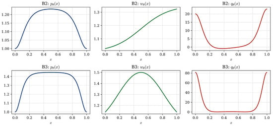
which provides exact eigenpairs for all modes. The coefficient bounds used in the benchmarks are listed in Table 4; Figure 1 shows the coefficients of B2 and B3.
Table 4.
Benchmark problems (Dirichlet conditions). ; , are the minima on .
Figure 1.
Activation-generated coefficients of benchmarks B2 (top) and B3 (bottom). The potential is the manufactured potential (20); it is the function used in all computations.
4.2. Error Measures and Second-Order Convergence
For mesh sizes with , the experimental order of convergence is computed with the actual mesh ratio,
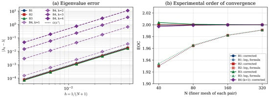
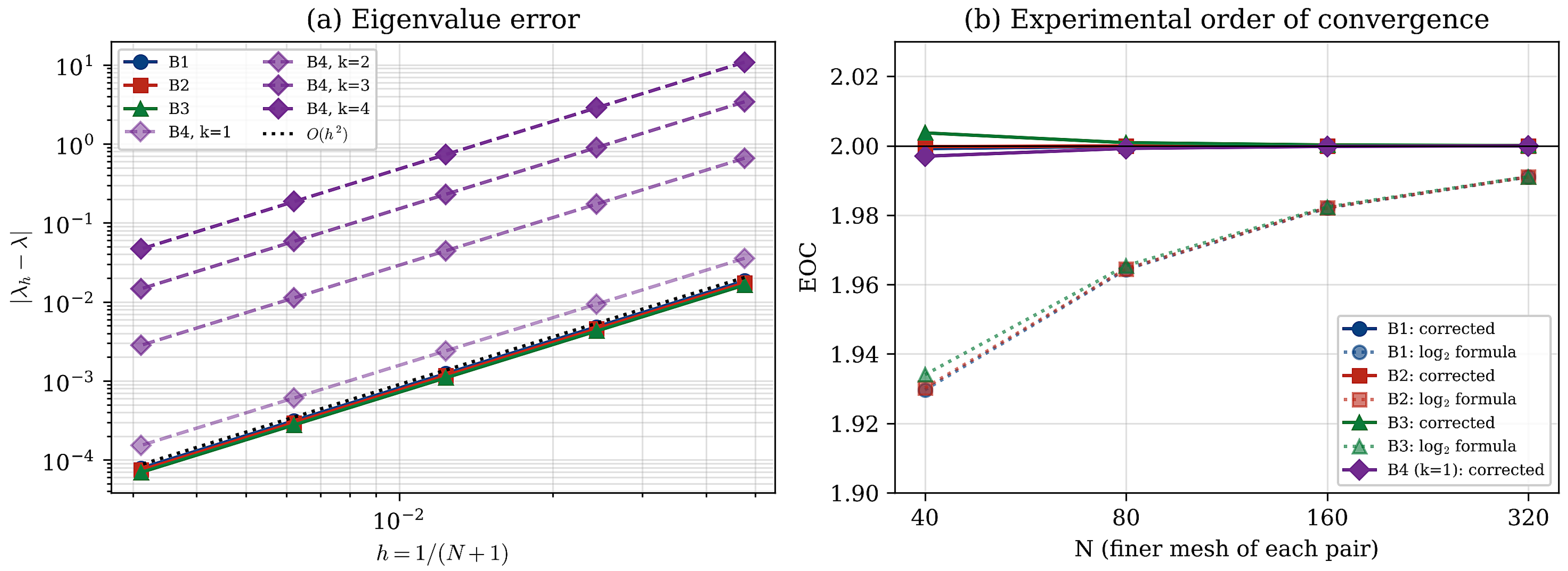
where . The frequently used shortcut , which tacitly assumes ; since for the first refinement, it underestimates the order (it gives 1.930–1.991 for the same errors). With (22), the same errors give orders within of 2 at every level (Table 5). Eigenfunction errors use the computed vector and the exact eigenfunction sampled at the nodes, both normalized by (12) with , . We report , the relative weighted error (i.e., , since ), and the unweighted .
Table 5.
Benchmarks B1–B3, first mode (). EOC from (22).
The relative eigenvalue error is ; since , is also the relative weighted error.
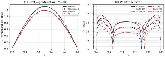
For B1, the discrete eigenvector coincides with up to rounding, so the eigenfunction errors are at the level of machine precision; the eigenvalue error is the familiar term. For B2 and B3, the eigenfunction errors decrease by a factor close to four per refinement. Figure 2 and Figure 3 show the eigenfunctions, pointwise errors, and convergence.
Figure 2.
(a) Exact and computed first eigenfunctions of B2 and B3 at (both normalized by (12)); (b) pointwise errors for , decreasing by a factor of about four per refinement.
Figure 3.
(a) Eigenvalue errors for B1–B3 () and B4 () with an reference line; (b) experimental order of convergence computed with the actual mesh ratio (22) (solid) and with the shortcut, which assumes (dotted).
4.3. Independent Benchmark B4: Higher Modes, Orthogonality, and Extrapolation
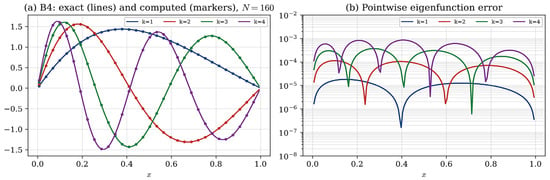
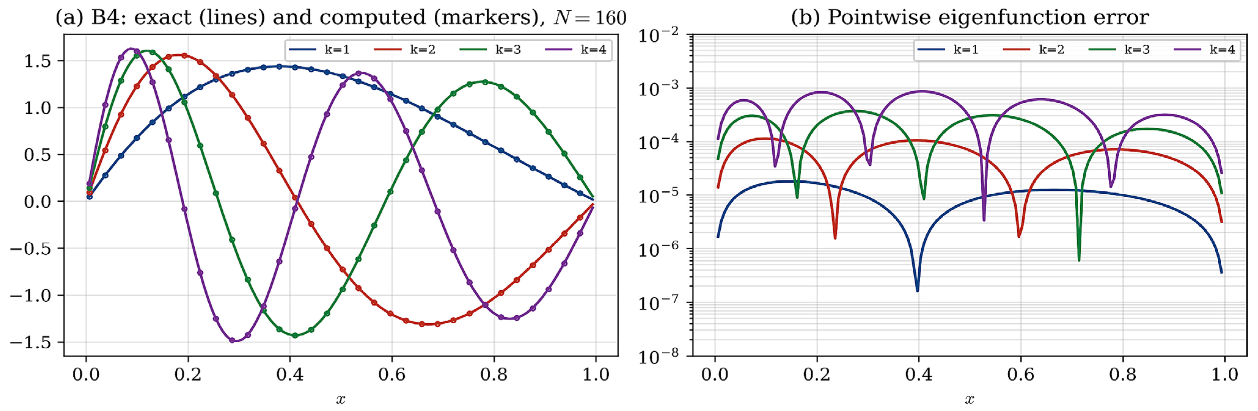
Table 6 shows second-order convergence for every mode, with EOC above 1.99 from onwards, and errors growing with as discussed after Theorem 2. The off-diagonal entries in Table 7 are at rounding level, as guaranteed by Lemma 1 (largest off-diagonal magnitude ). Because the error has an expansion in even powers of , one Richardson step with the true mesh ratio , , raises the order to four: for the extrapolated errors are , , , (orders 3.974, 3.984, 3.991), and for , , , . Figure 4 shows the modes and pointwise errors.
Table 6.
Benchmark B4, modes , with exact eigenvalues (21) , , , . Relative error (here ); EOC with respect to the previous mesh.
Table 7.
Discrete weighted Gram matrix for B4, .
Figure 4.
Benchmark B4 at : (a) exact (lines) and computed (markers) eigenfunctions for ; (b) pointwise errors.
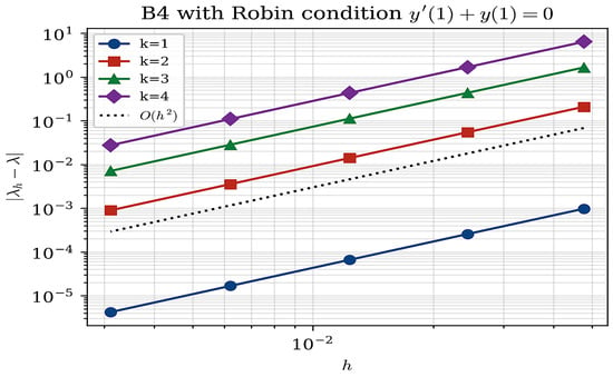
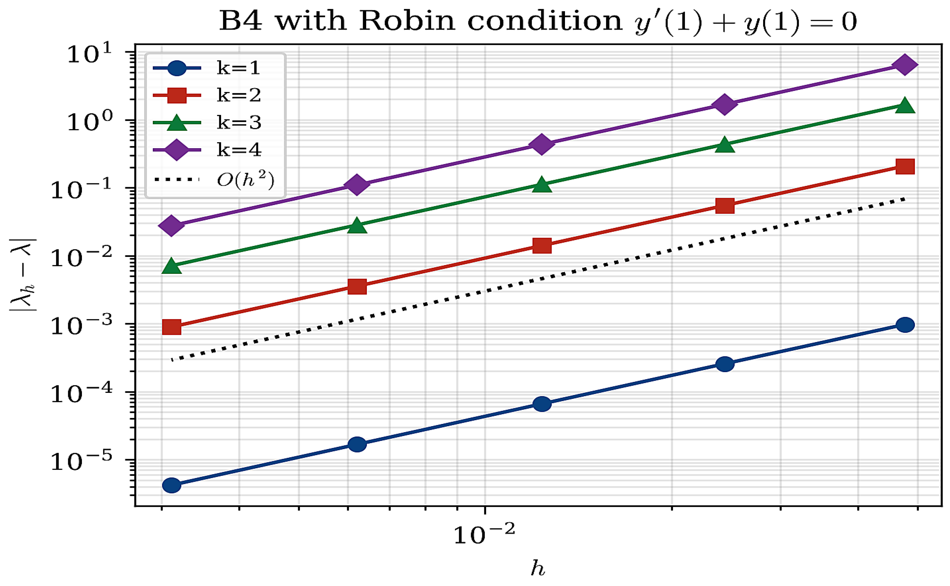
4.4. Robin Boundary Condition
To test the half-cell treatment (15), we keep the B4 coefficients and replace the right condition by (). With and , the condition becomes the scalar equation , which is solved to machine precision by bracketing. The resulting values , , , agree with Pyslise [23] to within . Table 8 and Figure 5 confirm second-order convergence for all four modes.
Table 8.
Robin condition with B4 coefficients: errors and EOC.
Figure 5.
Second-order convergence of the half-cell Robin discretization (15) for B4 with .
4.5. Comparison with Established Solvers
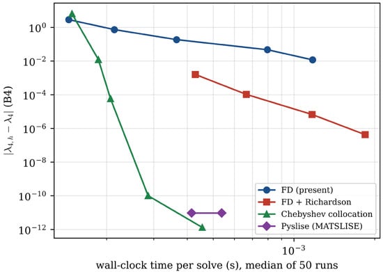
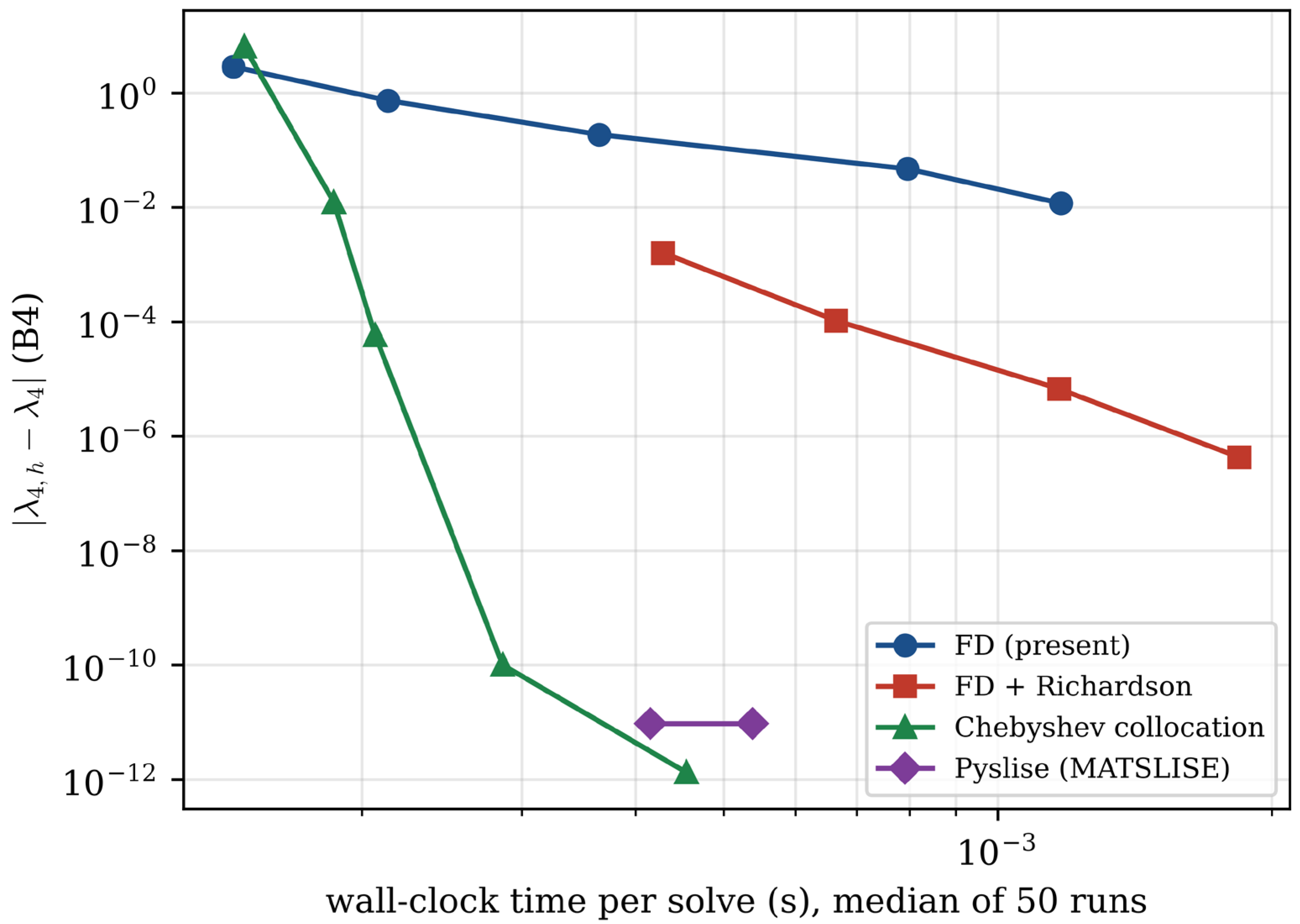
Table 9 and Figure 6 compare, for B4, the present scheme, the scheme with one Richardson step (using meshes and , so that is exactly halved), Chebyshev collocation on Gauss–Lobatto points [24], and Pyslise [23], the Python successor of MATSLISE [22]. Times are wall-clock time per solve for the first four eigenvalues on a single thread, reported as the median of 50 repeated solves after one warm-up call, on an Intel Xeon processor at 2.80 GHz (Python 3.13, NumPy 2.5, SciPy 1.18, Pyslise 3.2.2); they depend on the machine and serve only for relative comparison.
Table 9.
Accuracy and cost for B4: errors in and and time per solve (ms).
Figure 6.
Error in of B4 against time per solve for the four methods of Table 9. Times are medians of 50 repeated solves (Section 4.5).
For fixed smooth coefficients, the conclusion is unambiguous: Chebyshev collocation reaches in with , and Pyslise reaches about at comparable cost, whereas the second-order scheme needs for . Richardson extrapolation narrows but does not close this gap. We therefore do not recommend the present scheme when only eigenvalues for fixed smooth coefficients are required. Its advantages lie elsewhere: the pencil is symmetric definite and tridiagonal for every (Lemma 1); the derivatives (17) are exact for the computed eigenvalues and cost per parameter; the bounds of Theorem 3 hold at every mesh size; and the method extends unchanged to coefficients with limited smoothness, where spectral collocation loses its exponential convergence. Chebyshev collocation produces a nonsymmetric pencil, so the analogue of (17) requires left eigenvectors, and Pyslise does not provide parameter derivatives directly.
The Pyslise errors in Table 9 are identical for and . This is not an error floor of the reference values, which are evaluated from (21) in double precision with errors below (checked in 40-digit arithmetic). It is a floor of the general Sturm–Liouville interface of Pyslise, which first transforms the problem to Liouville normal form: the errors are the same for every tolerance from to and fall to about for , whereas for the same problem posed directly in normal form, on , Pyslise attains errors between and .
4.6. Verification of the GLT Symbol
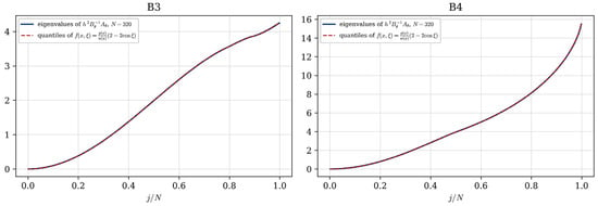
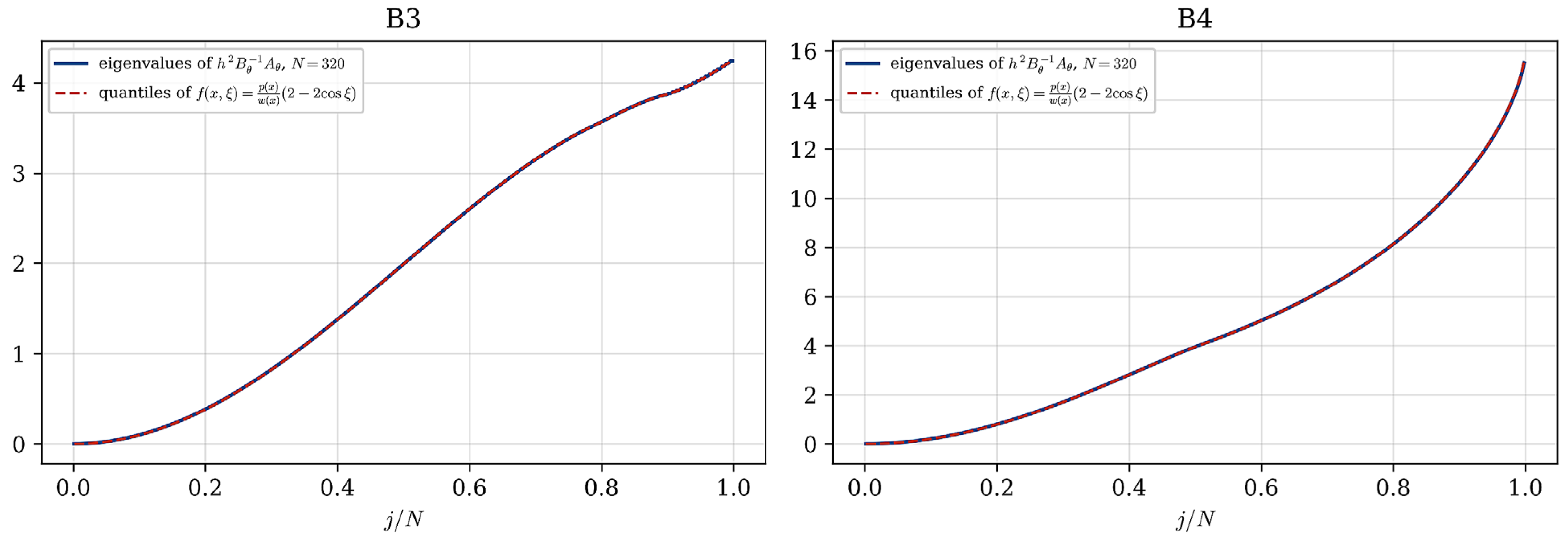
Figure 7 compares the sorted eigenvalues of for B3 and B4 at with the quantile function of the symbol (19), evaluated on a grid in . The maximum quantile gap, normalized by , decreases from to for B3 and from to for B4 as increases from 40 to 640, in agreement with Proposition 3.
Figure 7.
Sorted eigenvalues of (solid) and quantiles of the GLT symbol (dashed) for (B3) and (B4), .
4.7. Coefficient Perturbations
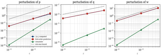
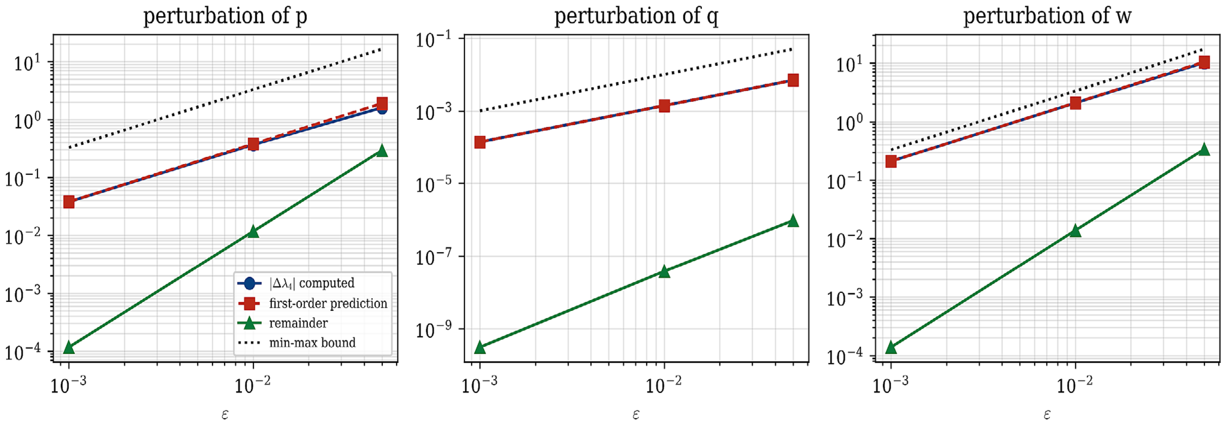
We perturb the B4 coefficients with the smooth profiles , and at . Table 10 reports the computed shifts of and , the first-order predictions from (17), and the bound (18) for (here, , or equals and ). The largest relative shift of is (p, ), (q, ), (w, ). All 36 perturbed eigenvalues (, nine perturbations) lie within the bounds of Theorem 3. The negative shift of under the -perturbation is not in conflict with monotonicity, because changes sign: by (16), the first-order shift is , and this integral is negative because the energy density carries more weight on , where , than on . The remainder (computed minus predicted) decreases by a factor of about 100 when decreases by 10, confirming that (17) is the exact first-order term (Figure 8).
Table 10.
Eigenvalue shifts for B4 () under the perturbations of Section 4.7: computed shifts , first-order predictions from (17), remainder for , and the interval for allowed by (18).
Figure 8.
Shift of for B4 under perturbations of , and : computed, first-order prediction (17), remainder (), and the min–max bound (18).
4.8. Activation-Parameter Identification
We now use the exact gradients for calibration. The coefficient family has six parameters ,
so that and for every (Proposition 1). Only and are activation-generated; the potential is affine. This is admissible because Proposition 1 imposes no sign condition on , but it limits the family: an affine cannot represent, for example, (see the misspecified test below). The target is . The data are the first eigenvalues and coefficient samples at equispaced points . The objective is
with and . Its gradient is assembled from (17) and the explicit derivatives of (23). We use L-BFGS-B (SciPy) with , starting point , and stopping tolerances and relative reduction (SciPy parameter ftol), with at most 1000 iterations. Algorithm 2 states the procedure.
| Algorithm 2. Activation-parameter calibration with exact eigenvalue gradients |
| Input: data |
| , ; family (23); ; weights , ; initial ; tolerances , ; . |
| Output: calibrated , final , , number of iterations. |
| 1: For : evaluate , , at nodes and half-nodes; admissibility holds by construction. |
| 2: Compute and with Algorithm 1. |
| 3: Compute from (17) for all , . |
| 4: Evaluate from (24) and by the chain rule. |
| 5: Perform an L-BFGS-B step to obtain . |
| 6: Stop when , or the relative decrease of is below ftol, or ; return . |
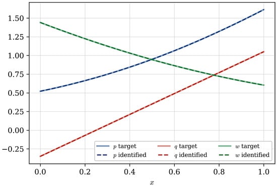
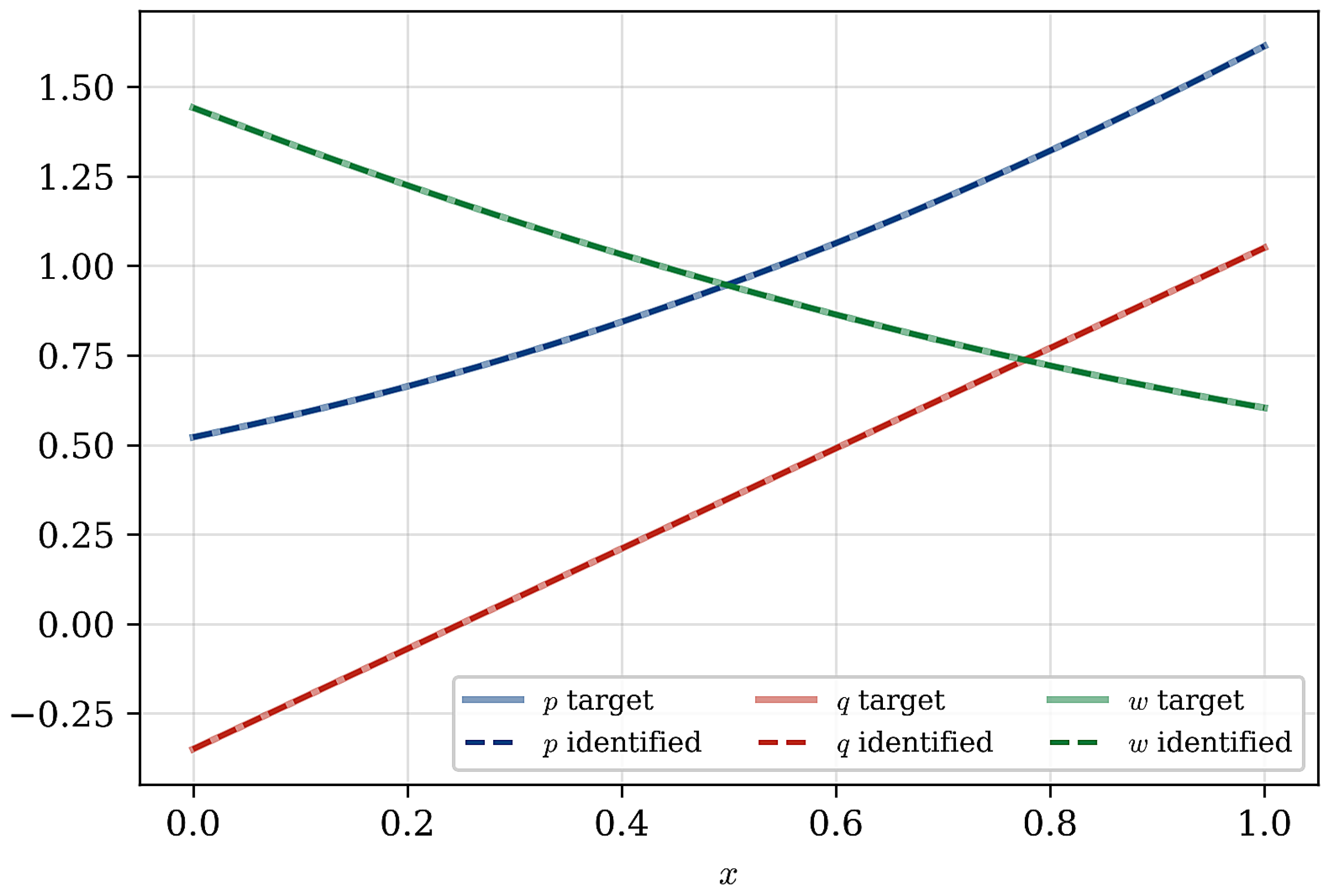
Table 11 summarises the results. In the noise-free case, (a) L-BFGS-B converges in 19 iterations to (this value is the regularization term ) with ; all parameters are recovered to within , the first four eigenvalues to relative accuracy , and the coefficient maps with root-mean-square errors (), (), (). With independent eigenvalue data, (b) the discretization error of (about relative at ) becomes a model error, and the largest parameter error rises to . Under noise (c), the mean estimates differ from by at most , with standard deviations between and . Relative to the standard errors s.d./, these deviations are below 1.3 standard errors for , , , and , and about two standard errors for and ( and ), so a small bias in the weight parameters cannot be excluded at this sample size. Figure 9 compares target and identified coefficients.
Table 11.
Identified parameters. (a) noise-free data from the same discretization; (b) eigenvalue data from Pyslise (tolerance ), i.e., without the “inverse crime”; (c) mean standard deviation over 50 replicates with 0.1% noise on eigenvalues and 1% noise on coefficient samples.
Figure 9.
Target (thick) and identified (dashed) coefficients for the noise-free same-family test (case (a) of Table 11).
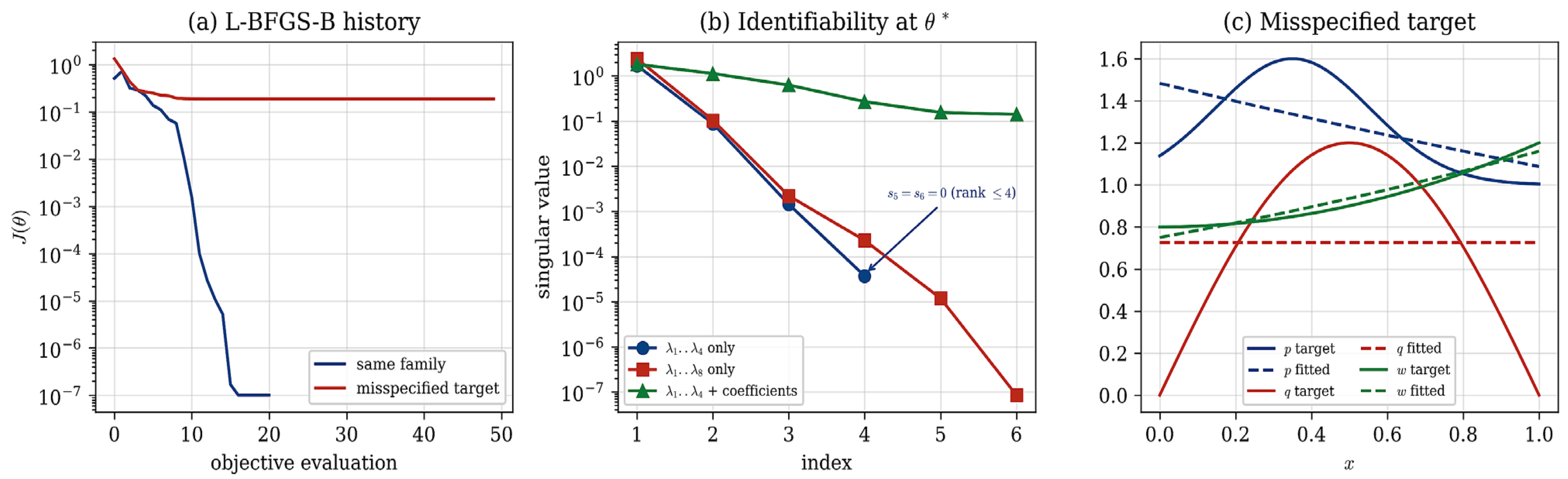
Identifiability. Table 12 lists the singular values of the Jacobian of the residual vector of (24) at . With eigenvalue data only, the Jacobian is ; for , its rank is at most four, so two directions in parameter space leave unchanged to first order, and the problem is not locally identifiable. Using eigenvalues restores full rank, but the smallest singular value is (condition number ), so identification is unstable. This is expected. Under the Liouville transformation , , , the problem becomes on , with a transformed potential determined by , and [1,10,18]. The spectrum therefore depends on and only through and , so , , and cannot be recovered separately even from the complete spectrum; Borg’s theorem [31] concerns the different question of recovering a potential from two spectra. Adding the coefficient samples gives a well-conditioned problem (condition number 12.9). In a multistart test with 20 initial points , the eigenvalue-only objective with reached in 0 of 20 runs (median error 0.85), whereas the combined objective (24) succeeded in 20 of 20 runs (largest error ).
Table 12.
Singular values of the residual Jacobian at .
Which data identify the parameters. The coefficient samples in (24) determine on their own: their Jacobian has full rank with condition number 8.8, and adding does not improve it (12.9). The main experiment therefore verifies the eigenvalue gradients and the solver; it does not show that spectral data identify the parameters. Table 13 shows when they do. Each data combination was tested from the same 20 random starts with ; with the ill-conditioned combinations are biased by about , because the regularisation then dominates the weakest directions, so for partial data, the regularisation must be reduced accordingly. Without eigenvalues, sampling only and , or a single value of each coefficient, leaves the Jacobian rank-deficient (ranks 4 and 3). Adding eigenvalues restores identifiability: with and sampled and unobserved, already recover all six parameters in 20 of 20 starts (largest error ), and one sample of each coefficient together with succeeds in 19 of 20 starts. These problems are, however, ill-conditioned (condition numbers to ), because by (16), the eigenvalues sense the coefficients mainly through weighted averages; for example, equals 0.974, 1.008, 1.015, 1.017 for , so the eigenvalues determine the mean level of far better than its slope.
Table 13.
Identifiability of the six activation parameters for different data combinations: rank and condition number of the residual Jacobian at , and L-BFGS-B success () from 20 random starts with .
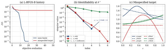
Misspecified target. Finally, the data are generated from , , , which do not belong to (23). The calibrated model matches the four eigenvalues to relative errors 1.19%, 0.26%, 0.47%, 0.41%, but the coefficient errors are substantial (root-mean-square 0.163, 0.372, 0.026 for , , ): an affine cannot represent , and the fit compensates in . Figure 10 shows the optimization histories, the singular values, and this fit. The example illustrates that the activation family acts as a restrictive model class: admissibility is guaranteed, but accuracy is limited by the expressiveness of the family.
Figure 10.
(a) Objective history of L-BFGS-B for the same-family and misspecified tests; (b) singular values of the residual Jacobian at (Table 12); (c) target and fitted coefficients for the misspecified test.
5. Discussion
What is classical and what is new. For fixed coefficients, the scheme, its preservation of self-adjointness, its second-order accuracy, and the growth of the error are classical [17,18,19], and our experiments confirm them for activation-generated coefficients, as expected for smooth, uniformly positive coefficients. The paper’s specific contributions are (C1)–(C6) of Section 1: an admissible parameterization under which every discrete problem is an unreduced symmetric-definite tridiagonal pencil; exact and cheap eigenvalue derivatives with respect to activation parameters; mesh-independent perturbation bounds; the GLT symbol of the parameterized pencil; and a calibration study whose identifiability analysis shows precisely which data determine the parameters.
Relation to learning-based methods. Approaches such as [35,36] represent eigenfunctions or coefficients by flexible maps. This construction offers a complementary building block: the coefficients are generated by the same activation functions, but the eigenpairs are computed by a structure-preserving solver whose derivatives are available in closed form. Embedding this block in a larger differentiable model, for example, one in which the coefficient generators are neural networks, is possible because (17) applies to any differentiable parameterization; this is not done here, and we make no claim about the performance of such models.
Limitations. The results are one-dimensional and assume smooth, uniformly positive , , bounded , and separated boundary conditions (Table 2). Singular endpoints, distributional weights [14], indefinite weights [15], fractional operators [16], and problems with discontinuous nonlinearities [13] require different analysis. The convergence proof covers Dirichlet conditions; for Robin conditions, only numerical evidence is given. The scheme is second order, and when only eigenvalues of fixed smooth problems are needed, spectral or Prüfer/CP-based codes are preferable (Section 4.5). Extending the approach to two-dimensional variable-coefficient and anisotropic operators would require a discretization that retains the symmetry of the discrete operator. Finally, eigenvalue data alone do not identify the six-parameter family, and they add information only when the coefficient data are partial (Table 13).
6. Conclusions
We have analyzed and tested a symmetric second-order finite-difference solver for Sturm–Liouville problems with activation-generated coefficients. The main findings are: (1) positivity enforced through activation offsets makes every parameter vector admissible, and every discrete pencil has simple eigenvalues; (2) with the experimental order computed from the true mesh ratio, all four benchmarks show orders between 1.9907 and 2.0037, and a half-cell Robin treatment is also second order; (3) discrete weighted orthogonality holds to the level of rounding error; (4) exact eigenvalue derivatives cost per parameter, agree with finite differences and converge at to the continuous sensitivities; (5) min–max bounds control eigenvalue shifts under coefficient perturbations at every mesh size; (6) the GLT symbol describes the entire discrete spectrum; and (7) with exact gradients, the calibration is reliable; complete coefficient samples determine the six activation parameters without eigenvalues, eigenvalues alone do not, and two to four eigenvalues supply the missing information when only part of the coefficient data is available, at the price of ill-conditioning. Extending the approach to two-dimensional variable-coefficient and anisotropic operators would require a different discretization; high-order block integrators developed for such elliptic problems [40,41] are natural candidates, provided the symmetry of the discrete operator can be retained. Also, future work will address higher-order and corrected schemes [19] within the same parameterized setting, noisy and partial coefficient observations with Bayesian calibration, and multidimensional operators, for which metric Sturm–Liouville theory in two dimensions [42] provides an analytical starting point.
Author Contributions
S.O.E.: software, writing—original draft, conceptualization, methodology; E.O.O.: methodology, formal analysis, writing—review and editing, supervision; E.M.A.: formal analysis, validation, writing—original draft, methodology; M.P.I.: validation, methodology, writing—review and editing, investigation; E.B.A.: formal analysis, writing—review and editing, validation, software; A.I.B.: software, investigation, formal analysis, writing—review and editing. T.S.F.: data curation; formal analysis; investigation; Writing—review and editing. F.H.O.: Investigation, Validation, Formal analysis, Writing—review and editing. Y.A.: validation, investigation, formal analysis, writing—review and editing. All authors have read and agreed to the published version of the manuscript.
Funding
This research received no external funding.
Data Availability Statement
The data supporting the findings of this study, including the Python code used to generate all numerical results, figures, and tables, are available from the corresponding author upon reasonable request.
Conflicts of Interest
The authors declare no conflicts of interest.
Abbreviations
The following list covers the abbreviations and software names used in the manuscript.
| Abbreviation | Meaning |
| CP | Constant perturbation |
| EOC | Experimental order of convergence |
| FD | Finite difference |
| GLT | Generalized locally Toeplitz |
| LAPACK | Linear Algebra Package |
| L-BFGS-B | Limited-memory Broyden–Fletcher–Goldfarb–Shanno algorithm with bound constraints |
| ReLU | Rectified linear unit |
| RMSE | Root-mean-square error |
| s.d. | Standard deviation |
| Software names | |
| Name | Description |
| MATSLISE | MATLAB R2024a package for solving Sturm–Liouville and Schrödinger equations |
| NumPy | Numerical Python; array-based numerical computing library |
| Pyslise | Python package for computing Sturm–Liouville and Schrödinger eigenpairs |
| SciPy | Scientific Python; scientific computing library |
| SLEDGE | Sturm–Liouville numerical solver using coefficient approximation |
| SLEIGN2 | Numerical code for solving Sturm–Liouville eigenvalue problems |
References
- Zettl, A. Sturm–Liouville Theory; Mathematical Surveys and Monographs; American Mathematical Society: Providence, RI, USA, 2005; Volume 121. [Google Scholar] [CrossRef] [Scilit]
- Marchenko, V.A. Sturm–Liouville Operators and Applications, revised ed.; AMS Chelsea Publishing, American Mathematical Society: Providence, RI, USA, 2011. [Google Scholar] [CrossRef] [Scilit]
- Daci, A.; Tola, S.; Çepa, N. Application of Sturm Liouville problem in the wave equation. Math. Model. 2023, 7, 76–79. [Google Scholar]
- Almalki, A. Sinc-Galerkin method for Sturm–Liouville problem with applications in quantum mechanics. J. Umm Al-Qura Univ. Appl. Sci. 2025. advance online publication. [Google Scholar] [CrossRef] [Scilit]
- Yaghmaie, F.A.; Modares, H.; Kiumarsi, B. On the numerical solutions to a certain Sturm–Liouville ODE for spectral filtering applications. In Proceedings of the 2025 European Control Conference (ECC), Thessaloniki, Greece, 24–27 June 2025; pp. 69–76. [Google Scholar] [CrossRef] [Scilit]
- Ahn, S.; Park, H. Examining the feasibility of the Sturm–Liouville theory for Ross recovery. Mathematics 2020, 8, 550. [Google Scholar] [CrossRef] [Scilit]
- De Oliveira, E.C.; Maiorino, J.E. Sturm–Liouville systems. In Analytical Methods in Applied Mathematics; Problem Books in Mathematics; Springer: Cham, Switzerland, 2024; pp. 169–195. [Google Scholar] [CrossRef] [Scilit]
- De Gregorio, S.; Lamberti, L.; De Gregorio, P. Some further insight into the Sturm–Liouville theory. Mathematics 2025, 13, 2405. [Google Scholar] [CrossRef] [Scilit]
- Derkach, V.; Malamud, M. Sturm–Liouville operator. In Extension Theory of Symmetric Operators and Boundary Value Problems, 2nd ed.; Operator Theory: Advances and Applications; Birkhäuser: Cham, Switzerland, 2026; Volume 309, pp. 545–659. [Google Scholar] [CrossRef] [Scilit]
- Karjanto, N.; Sadhani, P. Unraveling the complexity of inverting the Sturm–Liouville boundary value problem to its canonical form. Mathematics 2024, 12, 1329. [Google Scholar] [CrossRef] [Scilit]
- Migda, J.; Nockowska-Rosiak, M.; Migda, M. Properties of solutions of generalized Sturm–Liouville discrete equations. Bull. Malays. Math. Sci. Soc. 2021, 44, 3111–3127. [Google Scholar] [CrossRef] [Scilit]
- Chu, J.; Meng, G.; Wang, F.; Zhang, M. Optimization problems on nodes of Sturm–Liouville operators with Lp potentials. Math. Ann. 2024, 390, 1401–1417. [Google Scholar] [CrossRef] [Scilit]
- Potapov, D.K. Approximation to the Sturm–Liouville problem with a discontinuous nonlinearity. Differ. Equ. 2023, 59, 1185–1192. [Google Scholar] [CrossRef] [Scilit]
- Guo, H.; Qi, J. Sturm–Liouville problems involving distribution weights and an application to optimal problems. J. Optim. Theory Appl. 2020, 184, 842–857. [Google Scholar] [CrossRef] [Scilit]
- Ćurgus, B.; Derkach, V.; Trunk, C. Indefinite Sturm–Liouville operators in polar form. Integral Equ. Oper. Theory 2024, 96, 2. [Google Scholar] [CrossRef] [Scilit]
- Koyunbakan, H.; Shah, K.; Abdeljawad, T. Well-posedness of inverse Sturm–Liouville problem with fractional derivative. Qual. Theory Dyn. Syst. 2023, 22, 23. [Google Scholar] [CrossRef] [Scilit]
- Keller, H.B. On the accuracy of finite difference approximations to the eigenvalues of differential and integral operators. Numer. Math. 1965, 7, 412–419. [Google Scholar] [CrossRef] [Scilit]
- Pryce, J.D. Numerical Solution of Sturm–Liouville Problems; Clarendon Press: Oxford, UK, 1993; ISBN 978-0-19-853415-0. Available online: https://orca.cardiff.ac.uk/id/eprint/101057/ (accessed on 22 October 2026).
- Paine, J.W.; de Hoog, F.R.; Anderssen, R.S. On the correction of finite difference eigenvalue approximations for Sturm–Liouville problems. Computing 1981, 26, 123–139. [Google Scholar] [CrossRef] [Scilit]
- Bailey, P.B.; Everitt, W.N.; Zettl, A. Algorithm 810: The SLEIGN2 Sturm–Liouville code. ACM Trans. Math. Softw. 2001, 27, 143–192. [Google Scholar] [CrossRef] [Scilit]
- Pruess, S.; Fulton, C.T. Mathematical software for Sturm–Liouville problems. ACM Trans. Math. Softw. 1993, 19, 360–376. [Google Scholar] [CrossRef] [Scilit]
- Ledoux, V.; Van Daele, M.; Vanden Berghe, G. MATSLISE: A MATLAB package for the numerical solution of Sturm–Liouville and Schrödinger equations. ACM Trans. Math. Softw. 2005, 31, 532–554. [Google Scholar] [CrossRef] [Scilit]
- Baeyens, T.; Van Daele, M. The fast and accurate computation of eigenvalues and eigenfunctions of time-independent one-dimensional Schrödinger equations. Comput. Phys. Commun. 2021, 258, 107568. [Google Scholar] [CrossRef] [Scilit]
- Trefethen, L.N. Spectral Methods in MATLAB; Society for Industrial and Applied Mathematics: Philadelphia, PA, USA, 2000. [Google Scholar] [CrossRef] [Scilit]
- Liu, C.-S.; Chang, J.-R.; Shen, J.-H.; Chen, Y.-W. A boundary shape function method for computing eigenvalues and eigenfunctions of Sturm–Liouville problems. Mathematics 2022, 10, 3689. [Google Scholar] [CrossRef] [Scilit]
- Leibsle, F.M.; Rhee, N.; Bani-Yaghoub, M. A matrix-eigenvalue method to compute Sturm–Liouville polynomials. Mo. J. Math. Sci. 2022, 34, 19–29. [Google Scholar] [CrossRef] [Scilit]
- Mikhailov, M.D.; Vulchanov, N.L. Computational procedure for Sturm–Liouville problems. J. Comput. Phys. 1983, 50, 323–336. [Google Scholar] [CrossRef] [Scilit]
- Tilli, P. Locally Toeplitz sequences: Spectral properties and applications. Linear Algebra Appl. 1998, 278, 91–120. [Google Scholar] [CrossRef] [Scilit]
- Serra-Capizzano, S. Generalized locally Toeplitz sequences: Spectral analysis and applications to discretized partial differential equations. Linear Algebra Appl. 2003, 366, 371–402. [Google Scholar] [CrossRef] [Scilit]
- Garoni, C.; Serra-Capizzano, S. Generalized Locally Toeplitz Sequences: Theory and Applications; Springer Monographs in Mathematics; Springer: Cham, Switzerland, 2017; Volume 1. [Google Scholar] [CrossRef] [Scilit]
- Borg, G. Eine Umkehrung der Sturm-Liouvilleschen Eigenwertaufgabe: Bestimmung der Differentialgleichung durch die Eigenwerte. Acta Math. 1946, 78, 1–96. [Google Scholar] [CrossRef] [Scilit]
- Rundell, W.; Sacks, P.E. Reconstruction techniques for classical inverse Sturm–Liouville problems. Math. Comput. 1992, 58, 161–183. [Google Scholar] [CrossRef]
- Jiang, X.; Li, X.; Xu, X. Numerical algorithms for inverse Sturm–Liouville problems. Numer. Algorithms 2022, 89, 1287–1309. [Google Scholar] [CrossRef] [Scilit]
- Baev, A.V.; Mozgovykh, V.V. A method for solving the inverse Sturm–Liouville problem. Mosc. Univ. Comput. Math. Cybern. 2025, 49, 173–181. [Google Scholar] [CrossRef] [Scilit]
- Zhang, S.; Zu, J.; Zhang, J. Deep learning method for finding eigenpairs in Sturm–Liouville eigenvalue problems. Electron. J. Differ. Equ. 2024, 2024, 1–17. [Google Scholar] [CrossRef] [Scilit]
- Vigouroux, D.; Dalmau, J.; Béthune, L.; Boutin, V. Deep Sturm–Liouville: From sample-based to 1D regularization with learnable orthogonal basis functions. In Proceedings of the 42nd International Conference on Machine Learning, Vancouver, BC, Canada, 13–19 July 2025; Volume 267, pp. 61480–61497. Available online: https://proceedings.mlr.press/v267/vigouroux25a.html (accessed on 9 September 2026).
- Kato, T. Perturbation Theory for Linear Operators; Reprint of the 1980 Edition; Classics in Mathematics; Springer: Berlin/Heidelberg, Germany, 1995. [Google Scholar] [CrossRef] [Scilit]
- Nelson, R.B. Simplified calculation of eigenvector derivatives. AIAA J. 1976, 14, 1201–1205. [Google Scholar] [CrossRef] [Scilit]
- Courant, R.; Hilbert, D. Methods of Mathematical Physics; Interscience Publishers: New York, NY, USA, 1953; Volume 1. [Google Scholar] [CrossRef] [Scilit]
- Adeyefa, E.O.; Omole, E.O.; Shokri, A.; Nonlaopon, K. Numerical simulation of discretized second-order variable coefficient elliptic PDEs by a classical eight-step model. Results Phys. 2022, 41, 105922. [Google Scholar] [CrossRef] [Scilit]
- Adeyefa, E.O.; Omole, E.O.; Shokri, A.; Yao, S.-W. Hermite fitted block integrator for solving second-order anisotropic elliptic type PDEs. Fractal Fract. 2022, 6, 497. [Google Scholar] [CrossRef] [Scilit]
- Steinerberger, S. A metric Sturm–Liouville theory in two dimensions. Calc. Var. Partial. Differ. Equ. 2020, 59, 12. [Google Scholar] [CrossRef] [Scilit]

Disclaimer/Publisher’s Note: The statements, opinions and data contained in all publications are solely those of the individual author(s) and contributor(s) and not of MDPI and/or the editor(s). MDPI and/or the editor(s) disclaim responsibility for any injury to people or property resulting from any ideas, methods, instructions or products referred to in the content. |
© 2026 by the authors. Licensee MDPI, Basel, Switzerland. This article is an open access article distributed under the terms and conditions of the Creative Commons Attribution (CC BY) license.