Article

Integrating GIS and Official Statistics Using GISINTEGRATION

1
International Institute for Applied Systems Analysis (IIASA), 2361 Laxenburg, Austria
2
Big Data Lab, Imam Reza International University, Mashhad 178-436, Iran
3
Geo Intelligence Space, Belfast BT8 7UY, UK
4
Organisation for Economic Co-Operation and Development (OECD), 75016 Paris, France
*
Author to whom correspondence should be addressed.
AppliedMath 2025, 5(4), 166; https://doi.org/10.3390/appliedmath5040166
Submission received: 24 September 2025 / Revised: 5 November 2025 / Accepted: 17 November 2025 / Published: 2 December 2025

Abstract

Geospatial–statistical integration remains a persistent bottleneck for official statistics and applied spatial analysis. The GISINTEGRATION R package provides a modular, reproducible workflow for preprocessing, harmonizing, and linking heterogeneous GIS and non-GIS datasets, with export utilities that are compatible with common desktop GIS. This paper outlines the package architecture and demonstrates its use in two applications. The first integrates population statistics with newly introduced statistical output geographies for Northern Ireland, enabling rapid preparation of analysis-ready layers such as all usual residents and population density at Super Data Zones. The second links daily PM2.5 measurements from the U.S. EPA Air Quality System with county boundaries for California (July 2020) to produce policy-relevant indicators; spatial aggregation yielded valid monthly means for 46 of 58 counties (79.31%) and reduced variance from 40.716 (monitor level) to 5.777 (county means), improving signal stability and comparability. Across both cases, the workflow standardizes variable names, supports user-controlled overrides, identifies common keys, and performs quality checks, thereby reducing manual effort while increasing transparency and reproducibility. The results illustrate how standardized integration facilitates official statistical production, environmental monitoring, and evidence-based decision-making.

1. Introduction

Geographic Information System (GIS) data plays a pivotal role in numerous fields, including urban planning, environmental monitoring, disaster management, transportation, public health and particularly official statistics (see, for instance, [1,2,3,4,5]). GIS has been instrumental in mapping disease outbreaks, optimizing logistics networks, and identifying areas vulnerable to natural disasters [6,7].
From the perspective of a National Statistical Office (NSO), the primary focus is on non-GIS data, which serves as their core area of work. NSOs concentrate on economic, social, demographic, and environmental statistics. Recently, NSOs have begun to seriously explore the integration of GIS and statistical data (for more information, see, for instance, [8,9,10]). Though very useful, GIS data is not always available by itself; much non-GIS data has been produced and is being used for statistical office work on economics, social conditions, and health topics [10]. Most of these non-GIS datasets come from national censuses, surveys, and administrative records. They enrich and give background to an office’s spatial analysis [8].
Integrating GIS data with non-GIS data has emerged as a critical area of research and application in official statistics [11]. This integration enables comprehensive analyses that combine spatial and non-spatial dimensions, leading to more actionable insights. For example, linking demographic data with land-use maps can aid in urban development planning, while integrating weather data with agricultural statistics can improve crop management strategies [12,13]. However, the integration process is complex and often hindered by incompatible formats, inconsistent variable naming, and a lack of standardized tools [14].
Existing tools for data integration often focus on either GIS or non-GIS datasets in isolation, leaving a significant gap when addressing hybrid workflows [15]. Some tools offer partial solutions but are limited by high learning curves, lack of scalability, or incompatibility with diverse data sources [16]. Recent efforts in this domain highlight the transformative potential of effective GIS and non-GIS data integration [17]. Techniques such as record linkage, data harmonization, and advanced preprocessing have shown promise, but many of these approaches remain fragmented or inaccessible [18]. This fragmentation restricts the full utilization of data, curtailing advancements in critical fields such as public policy, environmental conservation, and disaster preparedness [19].
However, the GISINTEGRATION R package (Version 1.0) is the first comprehensive tool designed to bridge this gap [20]. By providing a robust and flexible framework for integrating GIS and non-GIS data, GISINTEGRATION addresses key challenges such as variable standardization, dataset harmonization, and scalable processing [15]. Its modular design and user-friendly interface empower users to efficiently preprocess and integrate data for a wide range of applications. This paper explores the package’s capabilities and its potential to revolutionize GIS workflows by addressing existing integration challenges and unlocking new opportunities for spatial analysis and decision-making.
To guide the reader, the remainder of the paper is organized as follows. Section 2 sets out the challenge of GIS data integration, summarizing the technical and institutional barriers that motivate our work. Section 3 introduces the GISINTEGRATION R package, detailing its architecture, core functions, and workflow, including preprocessing, harmonization, linkage, and export utilities. Section 4 demonstrates the package in practice through two applications; (i) to official statistics in Northern Ireland, and (ii) environment data, describing the datasets, integration steps, and resulting visualizations and analyses. Section 5 and  Section 6 conclude with key takeaways, limitations, and directions for future development and adoption across national statistical systems.

2. The Challenge of GIS Data Integration

Preprocessing and harmonizing the GIS databases from different sources have been the greatest long-time challenge in geospatial information management [21]. To the full extent of complexity with which geospatial information is characteristically laden, preprocessing, cleaning, unification, and integration of such data can be quite complicated [22]. The sources of this complexity are many: the multiplicity of different formats in which spatial data are collected; different scales, projections, and coordinate systems to boot; and diverse provenances for the data, such as satellite imagery, ground surveys, and more recently, user-generated content coming from mobile devices and social media platforms. With its own set of metadata, accuracy level, and cycle of updates, each dataset must be handled sensitively when integration is concerned [23]. Ensuring compatibility and consistency between the datasets requires not only simple data cleaning steps but also more advanced procedures such as coordinate transformation, conflation, and semantic reconciliation [24]. Furthermore, rapid technological and methodological advances mean that geospatial datasets are not only increasing in size but in complexity as well [25]. In the past, the absence of standardized tools for carrying out such multifaceted tasks impeded the capacity of professionals and researchers to execute truly comprehensive geospatial analyses. Often, analysts had to make do with somewhat disparate software tools or custom-coded scripts—a process that could be time-consuming, error-prone, and difficult to reproduce. Such fragmented efforts also work against the collaboration and sharing that is necessary to advance good practice in geospatial analysis. These barriers simply must be surmounted because the geospatial data is absolutely critical to a wide range of essential applications [26]. From that of urban planning and environment monitoring through disaster response and global health initiatives, near-infrared integrated geospatial data is integral. It informs policymakers in the formulation of policies, business strategy, and scientific research that will change lives and shape the future of our societies. The significant advancement for the field would be the completion of a comprehensive tool to streamline GIS data integration. This means that by offering a standardized, efficient, and robust way to pre-process, clean, unify, and integrate heterogeneous geospatial datasets, such a tool would lift the full limitations of geospatial analysis to allow intelligence that may be more accurate, insightful, and actionable from the wealth of data available.

3. Overview of the GISINTEGRATION Package

3.1. Package Structure

3.1.1. Preliminary Definition

Let D = { D 1 , D 2 , , D n } be a finite collection of GIS datasets. We assume each dataset D i ( i = 1 , , n ) consists of a set of observations (records) and a set of variables (attributes). The aim of the GISINTEGRATION package is to transform every D i into a harmonized dataset D i suitable for advanced spatial analyses in official statistics and data integration. Formally, we define the following preprocessing function:
Preproc : D D where D = { D 1 , D 2 , , D n } .
Each D i ( i = 1 , , n ) maintains the same number of records as D i but has standardized and cleaned variables/attributes.

3.1.2. Modularity and Adaptability

The GISINTEGRATION package is modular, allowing users to compose functions (or subroutines) that address specific tasks in a workflow. Let
F = { preproc , chzInput , create-new-data , preprocLinkageDBF , selVar }
be the set of available functions, each targeting a separate aspect of data preprocessing. Users can select which functions to apply based on the characteristics of their data (DBF stands for dBASE Database File, a tabular data format that originated with the legacy dBASE database management system). The GISINTEGRATION package offers several key functionalities:
  • Data Preprocessing: The preproc function standardizes variable names across datasets, ensuring consistency and reducing manual intervention. By addressing naming inconsistencies and discrepancies in data formats, preproc minimizes errors and prepares datasets for seamless integration. This step is crucial for ensuring compatibility across diverse GIS and non-GIS datasets, especially in large-scale projects.
  • User Consultation: The chzInput function allows users to specify variables that should retain their original names, providing flexibility in preprocessing. This feature empowers users to maintain domain-specific naming conventions where necessary, ensuring that critical variables retain their interpretability and relevance to stakeholders.
  • Final Data Preparation: The create-new-data function performs comprehensive preprocessing, including variable name harmonization, format adjustments, and the elimination of redundant or irrelevant data. This function outputs two refined data frames optimized for analysis, streamlining downstream workflows and reducing the need for additional cleaning steps.
  • DBF File Generation: The preprocLinkageDBF function automates data cleaning, normalization, and format transformations, making it possible to generate DBF files compatible with popular GIS software such as ArcGIS and QGIS. This capability ensures that datasets are ready for spatial visualization and advanced geospatial analyses, bridging the gap between data preprocessing and practical application.
  • Common Variable Identification: The selVar function identifies shared variables between datasets, facilitating the selection of blocking variables for linkage procedures. This step is essential for merging datasets from multiple sources, enabling robust data integration for tasks such as spatial modeling, demographic analysis, and environmental monitoring. Additionally, it aids in detecting potential inconsistencies or overlaps, enhancing data reliability.
  • Interactive User Experience: GISINTEGRATION includes an interactive interface that guides users through preprocessing steps. This feature reduces the learning curve for new users while allowing advanced users to customize the pipeline according to their needs, fostering a balance between simplicity and flexibility.

3.1.3. Efficiency and Compatibility

All functions in F are optimized with vectorized operations and robust algorithms. In practical terms, this ensures scalability for large n or datasets with a large number of records. The code is well-documented for ease of use and integrates seamlessly with popular R libraries such as sf, RecordLinkage, and stringr (for more information see [20]).

3.2. Workflow Description

Let us now represent the GISINTEGRATION workflow as a sequence of transformations applied to D . Let W denote the workflow, and let W ( D i ) be the output after all relevant functions have been applied to a single dataset D i . The pipeline for each dataset typically follows the following steps:
1.
Preprocessing GIS Datasets.
Call preproc ( D i ) to standardize variable names. This step normalizes naming conventions across D i :
D i ( 1 ) = preproc ( D i ) .
It resolves inconsistencies like mixed-case variable names or invalid characters.
2.
User-Specific Customization.
If the user wants to retain certain domain-specific variable names, apply:
D i ( 2 ) = chzInput ( D i ( 1 ) , varsToKeep ) ,
where varsToKeep is a subset of variable names that must remain unchanged.
3.
Final Data Preparation.
Consolidate all preprocessing steps into a final refined version:
D i ( 3 ) = create-new-data ( D i ( 2 ) ) .
This harmonizes variable formats (e.g., date, numeric) and removes redundant attributes, yielding a dataset ready for analysis.
4.
DBF File Preparation.
To facilitate geospatial visualization in software like ArcGIS or QGIS, generate DBF outputs:
preprocLinkageDBF D i ( 3 ) DBF files .
This ensures direct compatibility with common GIS platforms.
5.
Identifying Common Variables.
Finally, detect shared variables for linkage or merging:
commonVars = selVar D 1 ( 3 ) , D 2 ( 3 ) , , D n ( 3 ) .
This step is crucial for joining datasets and verifying consistency across multiple sources.
By composing these transformations, we can define the overall workflow W as:
W ( D i ) = selVar preprocLinkageDBF create-new-data chzInput preproc ( D i ) ,
implicitly assuming the multi-dataset scenario for the selVar function.
Figure 1 illustrates the overall GISINTEGRATION workflow, summarizing the key processes for data harmonization and integration. Panel (a) depicts the sequential preprocessing of individual GIS datasets, beginning with data import and variable standardization, followed by optional user decisions on retaining domain-specific names, and concluding with dataset restructuring and export into a standardized format. Panel (b) presents the subsequent multi-dataset integration process, where harmonized datasets are combined through common keys or mapping tables. This step includes validation, reconciliation, schema integration, and quality control checks to produce a unified, analysis-ready dataset.

3.3. Advanced Features in the Workflow

Beyond the steps listed above, GISINTEGRATION includes several auxiliary routines that enhance automation and interactivity:
  • Batch Processing:
    i { 1 , , n } , D i = W ( D i ) .
    This allows a user to process an entire collection D in one session, reducing manual work.
  • Interactive Debugging: Any errors or warnings during W ( D i ) provide detailed logs, indicating which function in F triggered the issue and offering suggestions for resolution.
  • Integration with R Markdown: Users can embed W ( D i ) calls inside literate programming documents, ensuring reproducibility and simplified reporting.
  • Custom Output Formats: In addition to DBF, the pipeline supports
    ExportTo ( D i ( 3 ) , { CSV , JSON , GeoJSON } ) ,
    enabling flexible dissemination of cleaned datasets. The GISINTEGRATION workflow ensures consistent, efficient, and reliable data integration across diverse GIS and non-GIS sources.

3.4. Positioning and Benchmarks

GISINTEGRATION builds upon established spatial data frameworks such as sf and terra, which provide robust functionality for geometry operations, coordinate reference system (CRS) management, and spatial joins. Rather than replacing these core packages, GISINTEGRATION extends their utility by automating repetitive preprocessing and harmonization tasks that are common in official statistics, environmental reporting, and multisource integration. Specifically, it streamlines schema alignment, variable standardization, crosswalk creation, and quality assurance, thereby enabling reproducible workflows for linking statistical and geospatial data.
Table 1 summarizes the relative performance and coding effort required to complete standard preprocessing and linkage tasks using conventional sf/terra code versus GISINTEGRATION. Benchmarks were conducted on representative datasets (Northern Ireland census and California PM2.5) to reflect typical integration workflows. Across all tasks, GISINTEGRATION reduced manual coding effort by an order of magnitude and generated standardized, auditable outputs with built-in coverage and variance reporting.
These results demonstrate that GISINTEGRATION complements existing spatial frameworks by providing an integrated, low-code layer for harmonizing large-scale statistical and geospatial datasets. The package leverages the computational efficiency of sf and terra while reducing human error, improving reproducibility, and ensuring that outputs meet interoperability and documentation standards required for official data dissemination.

3.5. Scope and Future Development

The current version of GISINTEGRATION focuses primarily on vector-based datasets—particularly tabular and polygonal data used in official statistics, censuses, and administrative boundary systems. This scope reflects the most frequent and operationally urgent integration needs in statistical offices and environmental monitoring institutions, where vector data represent the core link between spatial units and statistical attributes.
The package currently provides functionality for schema harmonization, attribute linkage, crosswalk creation, and governance-grade quality assurance. However, it does not yet natively handle raster or point-cloud data, such as remote sensing imagery, LiDAR, or high-resolution spatio-temporal grids. Similarly, complex spatial issues such as geometric conflation, topological correction, and scale harmonization across multiple spatial resolutions are beyond the current implementation.
Future versions of GISINTEGRATION will expand to address these more advanced integration challenges. Planned developments include:
  • Raster and remote-sensing integration: automated workflows for linking gridded data (e.g., population density, air quality, NDVI) with administrative boundaries using zonal statistics and spatial resampling.
  • Temporal harmonization: support for dynamic datasets with explicit time attributes, enabling longitudinal comparisons and versioned boundary handling.
  • Topological and scale reconciliation: integration of functions for detecting and resolving boundary overlaps, gaps, and mismatched resolutions.
  • Conflation tools: semi-automated matching of spatial features across differing data sources to support map alignment and geocoding validation.
These extensions will allow GISINTEGRATION to evolve from a harmonization-oriented toolkit toward a comprehensive spatial data integration framework capable of addressing raster–vector interoperability, multi-temporal data fusion, and topological quality control. The forthcoming release (v2.0) will prioritize these capabilities to broaden applicability across environmental, agricultural, and remote sensing domains while maintaining compatibility with the sf, terra, and stars ecosystems.

4. Application to Official Statistics

4.1. Population Census Data

We now illustrate how to apply W to official statistical data produced by the Northern Ireland Statistics and Research Agency (NISRA) for their latest Population Census (Census 2021) as a case study.

4.1.1. Dataset Description

The preprocessing pipeline significantly reduced the time and effort required for data preparation. The resulting integrated dataset was used to visualize population levels, such as absolute values (All Usual Residents) and population density (Number of Usual Residents per Hectare), by statistical output geographies (Super Data Zones [27]) in order to explore population dynamics by geographic distribution.
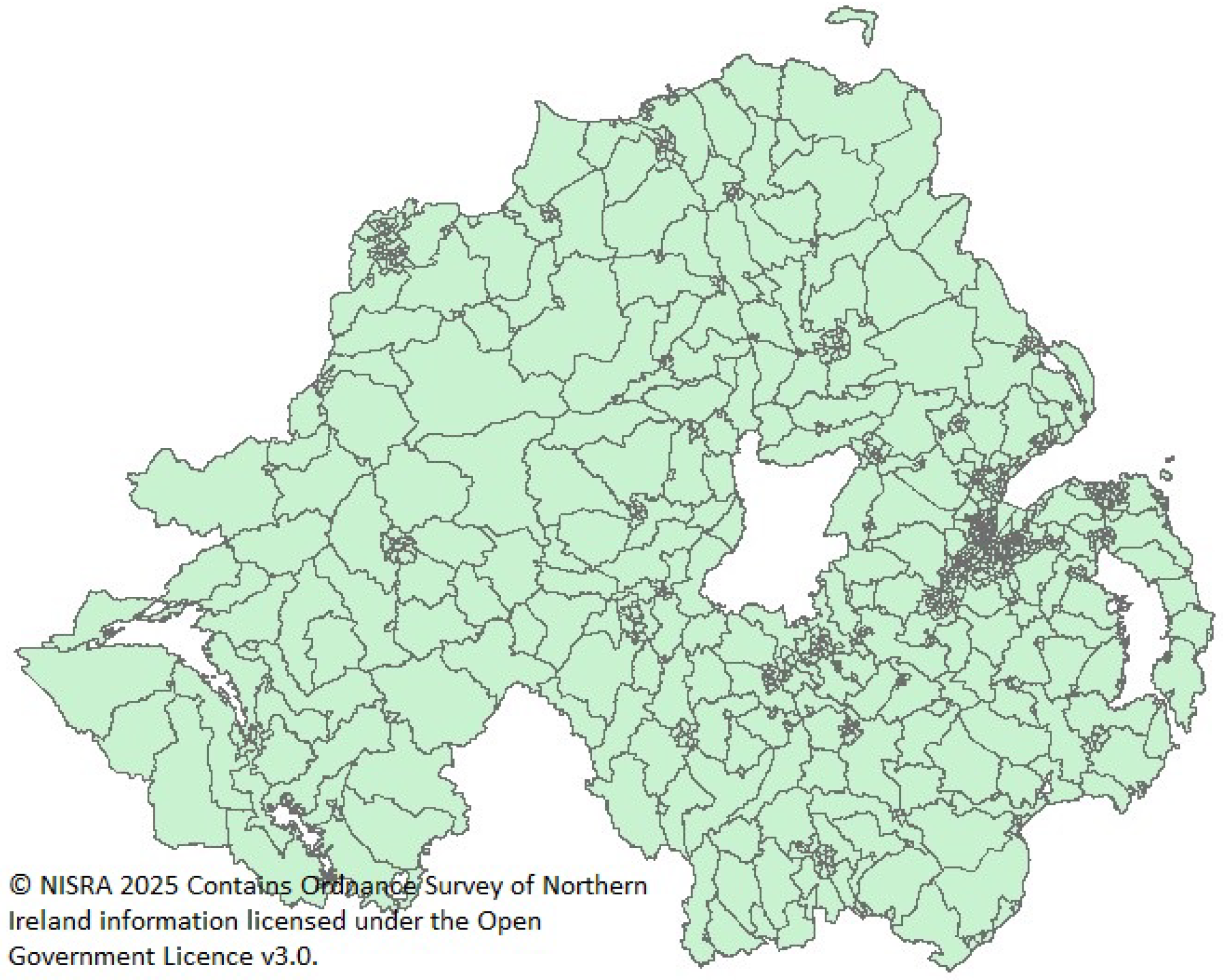
To support the dissemination of Census 2021 statistics, NISRA introduced two new statistical output geographies: Data Zones (DZ2021) and Super Data Zones (SDZ2021). Across Northern Ireland, there are 850 Super Data Zones (SDZ2021), within which 3780 Data Zones (DZ2021) are nested. These geographies are further nested within 80 District Electoral Areas (DEA2014) and 11 Local Government Districts (LGD2014) (see Figure 2).
Here, we consider the following datasets for demonstration:
  • Super Data Zones (SDZ2021) [27]:
    | D SDZ | = 500 ,
    a manageable dataset primarily used to test the GISINTEGRATION functionalities and refine workflow parameters.
  • Census 2021 Population Density Data (census-2021-ms-a14) [28]:
    D Census = population density values across multiple geographies .
    This dataset reflects the original structure provided by NISRA, including certain metadata sheets.
To integrate and merge these, let us define the following function:
M D SDZ , D Census D Integrated ,
where M encapsulates the GISINTEGRATION workflow W plus any additional linking logic (e.g., matching geographic codes). By applying W, each dataset is cleaned, standardized, and prepared for analysis, ensuring that statistical attributes (population density) align properly with the corresponding geospatial units (Super Data Zones).

4.1.2. Integration Results and Visualization in GISINTEGRATION

Let G be a finite set of geographic units relevant to the analysis (e.g., Super Data Zones, SDZ2021, within Northern Ireland). In this context,
G = { g 1 , g 2 , , g | G | } ,
where | G | = 850 for Super Data Zones (SDZ2021). Each g i G may itself include nested regions; for instance, there are 3 , 780 Data Zones (DZ2021) distributed across the entire set of SDZ2021 units.
Let A = { population density , area ( ha ) , all usual residents , } be a set of possible attributes or variables that can be linked to each g i . After the preprocessing pipeline described previously, we obtain an integrated dataset D int , which maps each geographic unit g i to a subset of attributes A i A . Formally,
D int : G 2 A ,
where D int ( g i ) = A i represents the attributes available (and harmonized) for that geographic unit.
  • Efficiency Gains
The transformation from raw data D to D int significantly reduces the manual effort required to clean and merge datasets. Once the pipeline W (as defined in the earlier sections) is applied,
D i D D i = W ( D i )
ensures that each D i is standardized. Subsequent integration of D i into D int is automated, thus minimizing user intervention and mitigating errors.

4.1.3. Population Density

The resulting integrated dataset can be used to analyze population density and its relationship to other variables (or any other attributes in A). Consider a function
f density : G R 0
that extracts the population density value for each geographic unit. Once f density is available within D int , a relational analysis (e.g., correlation, summary statistics) becomes straightforward.
Let A final A be the set of attributes a user decides to visualize after the integration process. The user may specify:
A final = { all usual residents , population density , } .
The system then generates a linked representation of G based on those attributes. In mathematical terms, for each g i G ,
V ( g i ) = { ( a , v i , a ) a A final } ,
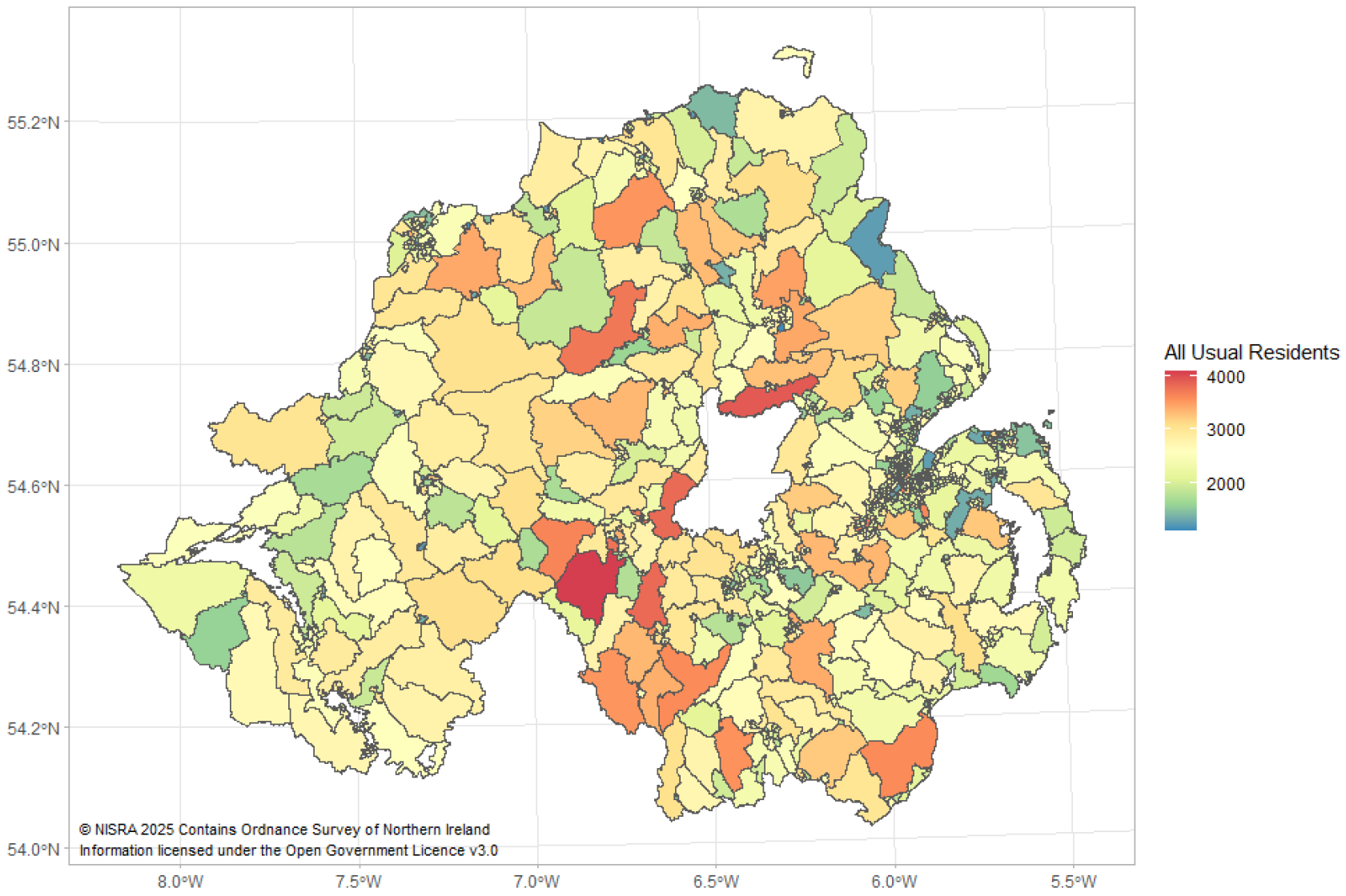
where v i , a denotes the observed value of attribute a for unit g i . Figure 3 exemplifies the result for the attribute all usual residents after data linkage. Figure 3 illustrates the full geographical context of Super Data Zones in Northern Ireland based on the linkage of data following the attribute chosen of all usual residents. This visualization is obtained after all data integration steps, at a stage which allows the user to select and focus on those specific attributes they are interested in displaying. Users will be able to choose and customize the geographic display so that salient points are made explicit, thereby enhancing the clarity and intelligibility of the spatial analysis.
Once D int is established, users can dynamically select and highlight any attribute a A final . This interactivity enhances clarity and interpretability of the final spatial analysis.

4.1.4. Multiple-Attribute Visualization

To visualize multiple attributes concurrently, define
A multi = { population density , area ( ha ) , road access , geographical borders } .
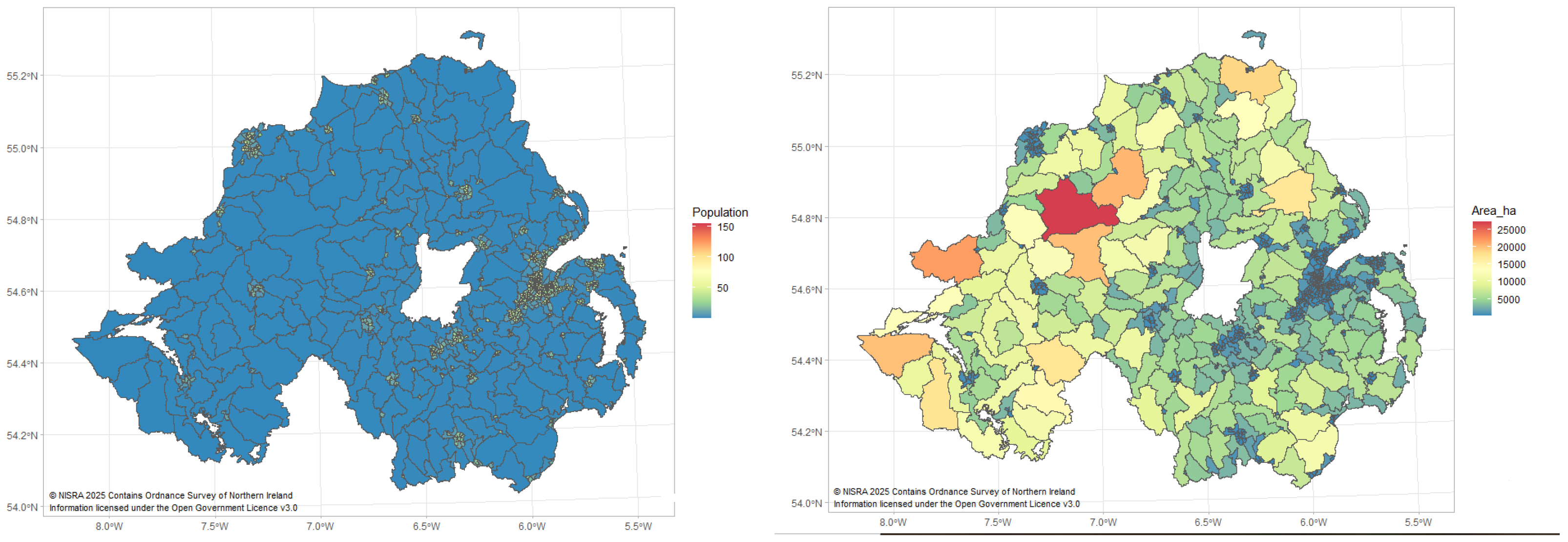
Each attribute is represented in a separate plot, effectively creating a 2-panel layout as shown in Figure 4 (Left plot: ( population density , g i ) and Right plot: ( area , g i ) ). Formally, let
P : A multi × G Plots
be a plotting function that produces a visual mapping of each attribute onto the relevant regions. Thus:
Additionally, a detailed view of integrating data is given by Figure 4 through two sets of distinct plots indicating different attributes. The plot to the left provides information on population density, showing how thinly or densely settled areas within each Super Data Zone are distributed. The plot on the right gives the size of the statistical output geography in hectares (ha), which allows an assessment of how big an area is in terms of its physical coverage. All these integrated datasets, from the steps of pre-processing to the point of data linkage, are handled by the GISINTEGRATION package. Such automation would bring in its wake seamlessness and efficiency in workflow with minimum manual intervention and error handling possibilities reduced. However, users are at liberty to choose any number of attributes of interest. An analysis can be customized and extracted for the purpose of research questions or policymaking needs. Potential alternative preprocessing steps to be automatically undertaken by the system in integrating diverse data attributes could enable the derivation of much more accurate and insightful spatial analyses that could be acted upon, hence enhancing decision-making and resource allocation within the scope of official statistics.
All relevant transformations leading to these visualizations,
f density , f area ,
are handled by the GISINTEGRATION pipeline W, ensuring consistency and reducing the scope for human error. This automation empowers researchers to integrate numerous attributes seamlessly and tailor the final outputs to specific research or policy objectives.
By coupling flexible attribute selection with automated data preprocessing, official statistical agencies can derive more accurate, insightful, and actionable spatial analyses. This advanced integration informs data-driven decision-making on issues such as resource allocation, urban planning, and demographic policy.

4.2. Application: Integration of Air Quality Data with Administrative Boundaries

Daily measurements of fine particulate matter (PM2.5) were integrated with county-level administrative boundaries to produce policy-relevant and comparable indicators for California during July 2020. This application demonstrates the capability of spatial data integration for environmental monitoring and public policy assessment. The following data sources are used for this application:
  • PM2.5: U.S. Environmental Protection Agency (EPA) AirData, Air Quality System (AQS) Daily Summary files for parameter 88101 (PM2.5, FRM/FEM mass), year 2020.
  • County boundaries: U.S. county polygons (FIPS-coded GeoJSON) distributed via Plotly Datasets, derived from the U.S. Census Bureau’s TIGER/Line shapefiles.
The EPA daily summary file for 2020 was filtered to include only records corresponding to California and the month of July. The retained variables included the date, arithmetic mean concentration, latitude, longitude, and county identifiers (code and name). A GeoDataFrame was constructed from the monitoring station readings using the WGS84 coordinate reference system (EPSG:4326).
County polygons were also imported from the FIPS-coded GeoJSON and subset to California (FIPS prefix 06). The coordinate reference systems of both datasets were aligned, followed by a spatial join to assign each monitor observation to its corresponding county polygon. Daily monitor-level observations were aggregated to compute county-level mean PM2.5 concentrations for July 2020. For each county, the arithmetic mean across all available monitor-days was calculated, and the number of contributing observations ( n obs ) was retained as an indicator of data coverage.

4.2.1. Visualization and Outputs

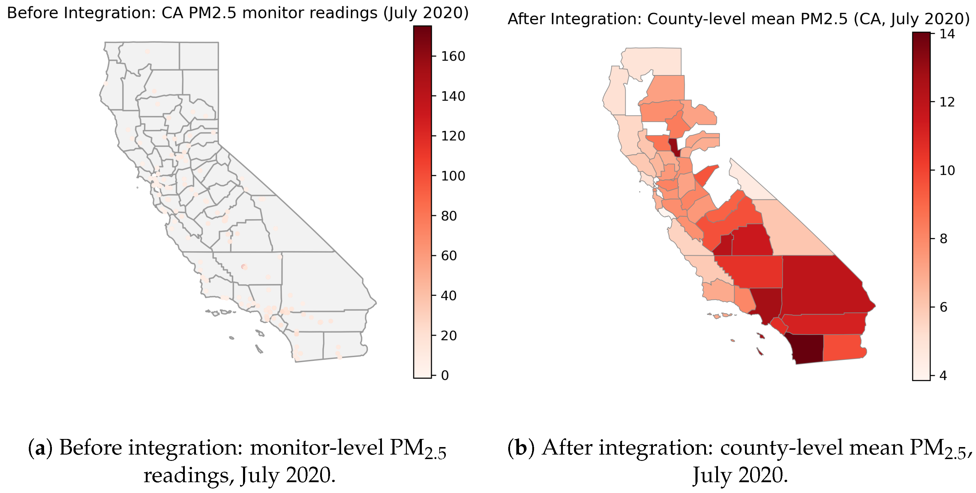
Two maps were produced to illustrate the integration process (Figure 5). Panel (a) displays the raw, monitor-level PM2.5 readings overlaid on county boundaries, highlighting the uneven spatial distribution of monitoring stations. Panel (b) presents the aggregated, county-level July mean PM2.5 values, yielding directly comparable and policy-relevant indicators aligned with administrative units.
  • The spatial aggregation clarifies geographic variation in PM2.5 exposure, with higher values observed in several counties in southern and central California. This transformation enhances interpretability and supports equitable air-quality policy design.
Quality control metrics were also designed to assess the robustness and interpretability of the aggregated results:
  • Coverage: Number and percentage of counties with at least one valid spatial assignment.
  • Variance reduction: Comparison of variance at the monitor level versus the county-level aggregated means, as an indicator of noise reduction and signal stability.
  • Descriptive statistics: Mean and median PM2.5 concentrations across all counties with sufficient coverage.

4.2.2. Results

Spatial integration substantially improved interpretability and produced stable, policy-relevant indicators at the county level. Valid July means were computed for 46 of California’s 58 counties (79.31%), while missing estimates were associated with counties lacking monitoring stations or having incomplete data. Variance decreased from 40.716 at the monitor level to 5.777 after aggregation, indicating effective noise reduction and improved signal stability. The mean county-level PM2.5 concentration was 8.03 µg/m3, with a median of 7.67 µg/m3, suggesting modest right-skewness driven by a few higher-concentration counties. Higher mean values were clustered in specific counties, reflecting spatial variation consistent with emission sources, topography, and meteorological influences.

5. Discussion

This paper demonstrated how a single, standardized workflow can support two very different integration problems: (i) linking Population Census statistics to newly introduced statistical output geographies (SDZ2021) in Northern Ireland, and (ii) aggregating air-quality observations (PM2.5) to county units in California. Although the domains, data models, and output uses differ, both applications highlight common integration challenges and show how GISINTEGRATION reduces manual effort, improves transparency, and yields analysis-ready, policy-relevant outputs.

5.1. Lessons from Population Census Integration

Integrating Census 2021 statistics with SDZ2021 in Northern Ireland illustrates several benefits for official statistics:
  • Rapid alignment with evolving geographies. NSOs frequently revise output geographies (e.g., DZ2021 and SDZ2021). By automating variable harmonization and schema reconciliation, GISINTEGRATION shortens the lag between geographic releases and the availability of analysis-ready statistical layers.
  • Traceability and reproducibility. Renaming, selection, and export steps are logged and repeatable, which is critical when disseminating official statistics and updating products as methods or source tables evolve.
  • Flexible attribute linkage. The workflow makes it straightforward to attach multiple attributes (e.g., all usual residents, population density, area) to the same spatial units, enabling multi-attribute visualization and downstream modeling.
  • Interoperable outputs. Standards-compliant DBF/CSV/GeoJSON exports allow immediate use in common GIS tools (ArcGIS/QGIS) and web mapping stacks, facilitating internal analysis and public communication.
At the same time, the census use case underscores domain-specific concerns:
  • Geographic change management. Newly defined zones require robust crosswalks to legacy geographies for time series comparability. Maintaining concordances and versioned metadata is as important as the one-off linkage.
  • Modifiable Areal Unit Problem (MAUP). Indicators such as density or rates depend on zoning systems and scale. Although the package standardizes processing, analysts must still interpret results in light of MAUP and consider sensitivity analyses across geographies (e.g., SDZ vs. DZ).
  • Key discovery and semantic alignment. Even within one statistical system, code lists, field names, and formats can vary across tables and vintages. Automated key/variable discovery (selVar) reduces brittle, hand-coded joins and avoids silent mismatches.
Overall, the Northern Ireland application shows how standardized preprocessing accelerates the production of authoritative, transparent geographic statistics, while preserving the controls and audit trails NSOs require.

5.2. Lessons from Air-Quality Integration

The California PM2.5 example demonstrates complementary strengths in an environmental-monitoring context:
  • Policy alignment through spatial aggregation. Aggregating monitor readings to counties produces indicators aligned with decision-making units, improving interpretability for health and regulatory uses.
  • Stability gains. Variance reduction from monitor-level values to county means indicates improved signal stability, aiding communication and comparisons across jurisdictions.
  • Coverage diagnostics. Retaining counts of contributing observations provides an explicit measure of data sufficiency and helps flag counties that may require alternative estimation strategies.
Domain-specific cautions include:
  • Uneven monitoring networks. Spatial clustering of monitors may bias county means. Where coverage is sparse or absent, model-based fusion (e.g., satellite products, reanalysis) or small-area estimation can complement direct aggregation.
  • Exposure representativeness. Simple arithmetic means do not capture diurnal patterns, episodic events, or population-weighted exposure; additional weighting or temporal smoothing may be warranted depending on the question.

5.3. Cross-Cutting Themes

Across both applications, several themes generalize beyond the specific datasets:
  • Standardization before sophistication. Routine—but error-prone—steps (naming, typing, key discovery, export constraints) are the bottleneck. Automating these with auditable logs unlocks analyst time for interpretation and advanced methods.
  • Governance-grade metadata. Reliable integration depends on versioned geographies, documented concordances, and explicit CRS handling. Embedding these artifacts in the pipeline improves institutional memory and reproducibility.
  • Interoperability as a design goal. Outputs that “just work” in mainstream GIS and analysis environments reduce friction for both specialists and non-specialists, speeding dissemination.

5.4. Limitations and Sensitivities

While GISINTEGRATION streamlines preprocessing and linkage, important limitations remain:
  • Data quality and representativeness. Integration cannot compensate for missingness, measurement error, or siting bias. Diagnostics (coverage, variance, outlier checks) should accompany any aggregated indicators.
  • Geographic dependence of results. MAUP and boundary updates can shift indicator values; where feasible, provide multi-scale views or stability checks across alternative zonations.
  • Scope of current implementation. The present focus is vector/tabular data. Raster integration, temporal versioning of boundaries, and conflation/topological correction are flagged for future development.

5.5. Implications for Producers and Users

For NSOs and public agencies, the population and air-quality cases suggest practical steps: adopt standardized preprocessing to shorten publication timelines; publish concordances and QA summaries alongside indicators; and provide interoperable exports to maximize reuse. For researchers and policymakers, the ability to link multiple attributes to consistent spatial units—and to understand uncertainty and coverage—improves the quality of evidence used in planning, equity assessments, and environmental health analyses.
In sum, the two applications together show that a uniform, auditable integration pipeline can serve both official statistical production and environmental monitoring, yielding outputs that are faster to produce, easier to trust, and simpler to communicate.

6. Conclusions

Effective use of geospatial information in official statistics depends on reliable, transparent, and reproducible data integration. The GISINTEGRATION package addresses this requirement through a structured pipeline that standardizes variables, supports user-controlled exceptions, reconciles schemas, and exports interoperable outputs suitable for mainstream GIS environments. The two applications presented—linking population statistics to Super Data Zones in Northern Ireland and aggregating PM2.5 observations to California counties—demonstrate that the same workflow generalizes across domains, data models, and administrative geographies.
In the Northern Ireland example, the package expedited the construction of analysis-ready layers at newly defined statistical geographies, facilitating population-level visualization and multi-attribute exploration. In the air-quality example, integration at county level produced directly comparable indicators that are usable for policy analysis and communication. Aggregation increased interpretability and stability, with variance decreasing from 40.716 at monitor level to 5.777 for county means and coverage achieved for 79.31% of counties in July 2020. These results underscore the value of standardized integration for revealing spatial patterns, enabling fair comparisons, and supporting downstream modelling and dissemination.
Several limitations warrant attention. Integration quality depends on the completeness and spatial representativeness of source data, the availability of robust keys or concordances, and careful handling of coordinate reference systems. In environmental settings, siting bias and missing monitors can affect county-level estimates, and simple arithmetic means do not capture exposure timing or uncertainty. In official statistics, evolving geographies require sustained maintenance of crosswalks and metadata.
Future development should expand input/output coverage (e.g., additional vector/raster formats), strengthen uncertainty propagation and diagnostics, and add options for population weighting, temporal smoothing, and model-based fusion with satellite or reanalysis products. Enhanced metadata management, validation reports, and API connectors to statistical and geospatial repositories would further support institutional adoption. By lowering the technical barriers to harmonization and linkage, GISINTEGRATION contributes a practical foundation for scalable geospatial–statistical production across national statistical systems and applied research.

Author Contributions

Conceptualization, H.H., L.M.M., S.S. and S.M.; methodology, H.H., L.M.M., S.S. and S.M.; writing—review and editing, H.H., L.M.M., S.S. and S.M. All authors have read and agreed to the published version of the manuscript.

Funding

This research did not receive external funding.

Data Availability Statement

The original data presented in the study are openly available in https://www.nisra.gov.uk/.

Conflicts of Interest

The authors declare no conflicts of interest.

References

  1. Agrawal, S.; Gupta, R.D. Web GIS and its architecture: A review. Arab. J. Geosci. 2017, 10, 518. [Google Scholar] [CrossRef]
  2. Dhurandhar, P.; Tamrakar, A.; Patra, J.P. Review on GIS-based online information system for rural development in Chhattisgarh. Int. J. Health Sci. 2022, 6, 8226–8231. [Google Scholar] [CrossRef]
  3. Li, L.; Zhu, D.; Ye, S.; Yao, X.; Li, J.; Zhang, N.; Han, Y.; Zhang, L. Design and implementation of geographic information systems, remote sensing, and global positioning system–based information platform for locust control. J. Appl. Remote Sens. 2014, 8, 084899. [Google Scholar] [CrossRef]
  4. UN-GGIM. Future Trends in Geospatial Information Management: The Five to Ten Year Vision, 3rd ed.; Report by the United Nations Committee of Experts on Global Geospatial Information Management; UN-GGIM: New York, NY, USA, 2020; Available online: https://ggim.un.org/meetings/GGIM-committee/10th-Session/documents/Future_Trends_Report_THIRD_EDITION_digital_accessible.pdf (accessed on 10 November 2025).
  5. Vinueza-Martinez, J.; Correa-Peralta, M.; Ramirez-Anormaliza, R.; Franco Arias, O.; Vera Paredes, D. Geographic Information Systems (GISs) Based on WebGIS Architecture: Bibliometric Analysis of the Current Status and Research Trends. Sustainability 2024, 16, 6439. [Google Scholar] [CrossRef]
  6. Goodchild, M.F. Geographical information science. Int. J. Geogr. Inf. Syst. 1992, 6, 31–45. [Google Scholar] [CrossRef]
  7. Longley, P.A.; Goodchild, M.F.; Maguire, D.J.; Rhind, D.W. Geographic Information Science and Systems; Wiley: Hoboken, NJ, USA, 2015. [Google Scholar]
  8. Available online: https://storymaps.arcgis.com/collections/470ca804de874925aadb4db9e9eca293 (accessed on 10 November 2025).
  9. Available online: https://unstats.un.org/unsd/ccsa/isi/2019/introduction.pdf (accessed on 10 November 2025).
  10. Available online: https://www.un.org/geospatial/ (accessed on 10 November 2025).
  11. Available online: https://unece.org/DAM/stats/publications/2016/Issue1_Geospatial.pdf (accessed on 10 November 2025).
  12. Gong, H.; Simwanda, M.; Murayama, Y. An Internet-Based GIS Platform Providing Data for Visualization and Spatial Analysis of Urbanization in Major Asian and African Cities. ISPRS Int. J. Geo-Inf. 2017, 6, 257. [Google Scholar] [CrossRef]
  13. Jing, C.; Zhu, Y.; Fu, J.; Dong, M. A lightweight collaborative GIS data editing approach to support urban planning. Sustainability 2019, 11, 4437. [Google Scholar] [CrossRef]
  14. UNECE Working Paper on Statistics, Issue 10. Issues and Obstacles to the Greater Integration of Statistical and Geospatial Information Across the UNECE Region. Available online: https://unece.org/sites/default/files/2024-08/INGEST%20issues%20and%20obstacles%20WP_combined.pdf (accessed on 10 November 2025).
  15. Available online: https://statswiki.unece.org/spaces/GeoStat/blog/2024/02/14/437420257/Unlocking+the+Power+of+Geospatial+Data+with+GIS+Data+Integration+A+New+R+Package (accessed on 10 November 2025).
  16. Adouane, K.; Stouffs, R.; Janssen, P.; Domer, B. A model-based approach to convert a building BIM-IFC data set model into CityGML. J. Spat. Sci. 2020, 65, 257–280. [Google Scholar] [CrossRef]
  17. Amirebrahimi, S.; Rajabifard, A.; Mendis, P.; Ngo, T. A BIM-GIS integration method in support of the assessment and 3D visualisation of flood damage to a building. J. Spat. Sci. 2016, 61, 317–350. [Google Scholar] [CrossRef]
  18. Arroyo Ohori, K.; DiakitA, A.; Krijnen, T.; Ledoux, H.; Stoter, J. Processing BIM and GIS models in practice: Experiences and recommendations from a GeoBIM project in the Netherlands. ISPRS Int. J. Geo-Inf. 2018, 7, 311. [Google Scholar] [CrossRef]
  19. Beck, F.; Abualdenien, J.; Borrmann, A. An evaluation of the strict meaning of owl:sameAs in the field of BIM GIS Integration. CEUR Workshop Proc. 2021, 3081, 154–165. [Google Scholar]
  20. Hassani, H.; Marvian Mashhad, L.; Stewart, S.; Macfeely, S. GISINTEGRATION: An R Package for GIS Data Preprocessing and Integration. CRAN. Available online: https://cran.r-project.org/web/packages/GISINTEGRATION/index.html (accessed on 10 November 2025).
  21. Annoni, A.; Smits, P.C. Main problems in building European environmental spatial data. Int. J. Remote Sens. 2003, 24, 3887–3902. [Google Scholar] [CrossRef]
  22. Villa, P.; Molina, R.; Gomarasca, M.A. Data Harmonisation in the Context of the European Spatial Data Infrastructure: The HUMBOLDT Project Framework and Scenarios. In Earth Observation of Global Changes (EOGC); Springer: Berline/Heidelberg, Germany, 2013. [Google Scholar]
  23. Bordogna, G.; Kliment, T.; Frigerio, L.; Brivio, P.A.; Crema, A.; Stroppiana, D.; Boschetti, M.; Sterlacchini, S. A Spatial Data Infrastructure Integrating Multisource Heterogeneous Geospatial Data and Time Series: A Study Case in Agriculture. ISPRS Int. J. Geo-Inf. 2016, 5, 73. [Google Scholar] [CrossRef]
  24. Evelpidou, N.; Cartalis, C.; Karkani, A.; Saitis, G.; Philippopoulos, K.; Spyrou, E. A GIS-Based Assessment of Flood Hazard through Track Records over the 1886–2022 Period in Greece. Climate 2023, 11, 226. [Google Scholar] [CrossRef]
  25. Li, K.; Wang, M.; Hou, W.; Gao, F.; Xu, B.; Zeng, J.; Jia, D.; Li, J. Spatial Distribution and Driving Mechanisms of Rural Settlements in the Shiyang River Basin, Western China. Sustainability 2023, 15, 12126. [Google Scholar] [CrossRef]
  26. Ajami, A.; Kuffer, M.; Persello, C.; Pfeffer, K. Identifying a Slums’ Degree of Deprivation from VHR Images Using Convolutional Neural Networks. Remote Sens. 2019, 11, 1282. [Google Scholar] [CrossRef]
  27. Super Data Zone. Available online: https://www.nisra.gov.uk/support/geography/super-data-zones-census-2021 (accessed on 10 November 2025).
  28. Northern Ireland Statistics and Research Agency. Available online: https://www.nisra.gov.uk/publications/census-2021-person-and-household-estimates-for-data-zones-in-northern-ireland (accessed on 10 November 2025).
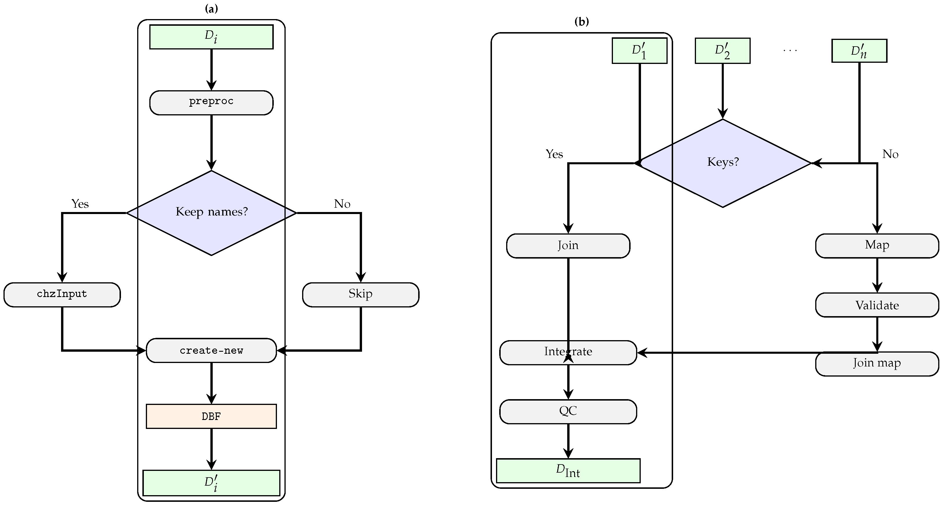
Figure 1. GISINTEGRATION workflow. (a) Single dataset preprocessing and export. (b) Integration of harmonized datasets into D Integrated .
Appliedmath 05 00166 g001
Figure 2. Geography preview of Super Data Zone across Northern Ireland. © NISRA 2025 Contains Ordnance Survey of Northern Ireland information licensed under the Open Government Licence v3.0.
Appliedmath 05 00166 g002
Figure 3. Geography preview of Super Data Zone across Northern Ireland after data linkage based on all usual residents as selected attribute. © NISRA 2025 Contains Ordnance Survey of Northern Ireland information licensed under the Open Government Licence v3.0.
Appliedmath 05 00166 g003
Figure 4. The left plot displays integrated population density, and the right plot illustrates area size. © NISRA 2025 Contains Ordnance Survey of Northern Ireland information licensed under the Open Government Licence v3.0.
Appliedmath 05 00166 g004
Figure 5. Spatial integration of daily PM2.5 observations with county administrative boundaries in California (July 2020). Panel (a) shows raw station-level readings, illustrating heterogeneity in monitor distribution. Panel (b) displays aggregated county-level means, revealing clear regional gradients and facilitating policy-relevant comparisons across jurisdictions.
Appliedmath 05 00166 g005
Table 1. Comparison of GISINTEGRATION with sf/terra on representative preprocessing tasks. LOC = lines of code.
Tasksf/terra (LOC)GISINTEGRATION (LOC)Added Value
Variable harmonization (15 files)90–1406–10Automated renaming, audit log
Key discovery and crosswalk buildCustom joins1–2Concordance generation
Spatial join and DBF-safe export20–402–3Standards-compliant fields
QA summary (coverage, variance)ManualAutoBuilt-in quality metrics
Batch pipeline (multi-dataset)Ad hoc loops1Reproducible processing
Disclaimer/Publisher’s Note: The statements, opinions and data contained in all publications are solely those of the individual author(s) and contributor(s) and not of MDPI and/or the editor(s). MDPI and/or the editor(s) disclaim responsibility for any injury to people or property resulting from any ideas, methods, instructions or products referred to in the content.