


Abstract
Introductory and intermediate electrical-engineering education commonly models fundamental circuit and device parameters, including inductance, capacitance, resistance, permeability, permittivity, conductivity, characteristic impedance, transformer turns ratio, machine constants, amplifier gain, resonant frequency, propagation velocity, and mutual inductance, as numerical constants. While this approximation is valid within the intended small-signal operating regime, it becomes methodologically incomplete when these coefficients exhibit measurable state dependence. This paper presents a comparative audit of thirteen such coefficients by systematically contrasting their textbook formulations with the established engineering literature and interpreting the results through two complementary frameworks: the JCGM GUM-6:2020 measurement-model methodology for omitted effects, and the Heckmann–Nye/Gasik multidomain coupling architecture for multi-axis physical interactions. The analysis demonstrates that mainstream engineering practice routinely exploits state-dependent coefficients without invoking new physical laws, and that relaxing the constant-coefficient assumption naturally introduces physically meaningful terms, including the inductive contribution , the capacitive counterpart , and the mutual-inductance term . The principal scientific contribution is the development and experimental validation of a unified theoretical and engineering framework for high-power resonant transformers and orthogonal Metglas AMCC-1000 paraformers. The proposed approach combines a new physics-based modal theory of octave () parametric excitation with simultaneous optimization of magnetic-core resonance, electrical resonance, nonlinear inductance modulation, resonant conductor lengths selected as integer multiples of the operating resonant wavelength, multi-stranded high-frequency Litz-wire windings, resonant capacitor synthesis, and the nonlinear magnetic characteristics of the AMCC-1000 amorphous core. The modal analysis demonstrates how coupled resonant eigenmodes and engineered state-dependent inductance can be used to satisfy the conditions for stable octave parametric excitation. Experimental results obtained from both the symmetric two-leg resonant transformer and the orthogonal paraformer are in close agreement with analytical predictions and numerical simulations, thereby validating both the proposed electromagnetic design methodology and the underlying modal theory.
1. Introduction
Electrical engineering has traditionally relied on purposefully simplified mathematical models. Treating inductance, capacitance, and resistance as constant parameters provides a compact and effective framework for analysing superposition, phasor relationships, transient responses, and impedance. Similar idealizations are routinely adopted for transformer turns ratios, transmission-line characteristic impedance, motor torque and back-electromotive-force constants, amplifier gains, and numerous other electrical quantities. These assumptions remain valid within a sufficiently small operating region, where parameter variations introduce negligible modelling error.
From a broader modelling perspective, however, these quantities should be regarded as effective parameters associated with a particular mathematical representation rather than as immutable physical properties of the underlying devices. For example, the familiar constitutive relation
is analytically convenient only when the inductance is treated as constant. In practical magnetic systems, the inductance generally depends on current, magnetic flux, mechanical displacement, temperature, excitation frequency, and other operating variables. Consequently, the conventional constant-coefficient formulation should be interpreted as a local approximation that is valid only within a well-defined operating regime.
The objective of this work is therefore not to challenge the usefulness of constant-parameter circuit models but, rather, to define the boundaries of their validity in a systematic and quantitatively traceable manner. The proposed methodology treats neglected state dependence as a measurement-model component in accordance with the principles of JCGM GUM-6:2020 [1], while simultaneously interpreting these dependencies within the multidimensional coupling framework originating from Heckmann and Nye [2] and subsequently extended through Gasik’s pentataxis representation for coupled physical phenomena [3].
The same metrological framework distinguishes between two complementary approaches for evaluating measurement uncertainty: Type A evaluation is based on the statistical analysis of repeated observations, whereas Type B evaluation relies on information obtained from calibration certificates, manufacturers’ specifications, previous measurements, scientific literature, or engineering judgement (JCGM 100:2008, Clauses 4.2 and 4.3) [4]. Within the comparative audit presented in this work, the constant coefficients adopted by conventional textbook models may be regarded as Type B estimates whose operating-point dependence is assumed to be negligible, whereas the experimentally observed state-dependent variations constitute Type A contributions that are frequently omitted from simplified engineering models. The present paper establishes the methodological framework for this comparison, while complete uncertainty budgets are reserved for subsequent experimental studies.
The central hypothesis investigated in this paper is that many electrical-engineering quantities commonly introduced as numerical constants—including inductance, capacitance, resistance, permeability, permittivity, electrical conductivity, characteristic impedance, transformer turns ratio, electromechanical machine constants, amplifier gain, resonant frequency, propagation velocity, and mutual inductance—are more accurately represented as state-dependent functions. The assumption of constant coefficients is therefore valid only within a verified small-signal operating region. Outside this region, the neglected parameter variations become measurable and may significantly influence circuit behaviour, modelling accuracy, and system performance.
To investigate this hypothesis, this paper introduces a comparative metrological and coupling-theory audit that identifies the operating conditions under which conventional constant-coefficient models remain adequate and the conditions under which state-dependent formulations become necessary. The proposed framework is intended to provide reviewers, researchers, educators, and practising engineers with a systematic criterion for assessing the applicability of conventional electrical models.
The remainder of this paper is organized as follows: Section 2 reviews the relevant literature on constant-coefficient modelling, international metrology, nonlinear and parametric electrical circuits, multidomain coupling theories, and resonant magnetic energy-conversion systems. Section 3 develops the theoretical framework, including the Heckmann–Nye/Gasik multidomain coupling architecture, the governing equations for state-dependent electrical parameters, and a new physics-based modal theory of octave parametric excitation in AMCC-1000 paraformers. Section 4 presents the comparative audit methodology together with thirteen representative constant-coefficient assumptions and their documented engineering validity limits. Section 5 applies the proposed framework to resonant transformer and paraformer design, including analytical modelling, numerical optimization, and experimental validation of Metglas AMCC-1000 prototypes. Section 6 discusses the methodological implications for electrical-engineering modelling and education, and Section 7 summarizes the principal conclusions.
2. Comparative Literature Review
The existing literature relevant to the present work can be broadly classified into five complementary research streams. Although these streams originate from different disciplines, they collectively establish the theoretical and methodological foundation for treating electrical-engineering parameters as state-dependent quantities rather than universal constants.
The first research stream comprises the classical textbook tradition of linear circuit and electromagnetic modelling. Standard circuit-analysis texts introduce inductance through
capacitance through
resistance through Ohm’s law, mutual coupling through a constant mutual inductance M, and resonance through
Similarly, textbooks on electromagnetics introduce permeability, permittivity, electrical conductivity, propagation velocity, and characteristic impedance as material or transmission-line parameters, while the electrical-machine and electronic-circuit literature commonly assumes constant transformer ratios, machine constants, and amplifier gains. The principal strength of these models lies in their analytical simplicity: by treating the governing coefficients as constants, the resulting equations become linear or locally linear and can be solved using classical analytical techniques. Their limitation, however, is that these coefficients represent local approximations valid only within a sufficiently restricted operating region rather than universal physical invariants.
The second research stream originates from international metrology, particularly the modelling framework established by JCGM 100:2008 [4] and JCGM GUM-6:2020 [1]. Although developed primarily for measurement science, these documents provide a rigorous methodology for constructing mathematical models by explicitly identifying input quantities, validity limits, neglected effects, model extensions, and associated uncertainty contributions. From the perspective of electrical engineering, this framework offers an objective criterion for determining when a simplified constant-coefficient model remains adequate and when additional state-dependent effects must be incorporated. Accordingly, the comparative audit presented in this paper adopts the GUM model-development methodology as its principal analytical framework.
The third research stream encompasses nonlinear electrical circuits and operating-point-dependent devices. Saturable reactors and magnetic amplifiers exhibit permeability and inductance that vary with magnetic excitation. Ferroresonant transformers and constant-voltage transformers intentionally operate within nonlinear magnetic regimes. Varactor-based parametric amplifiers employ voltage-dependent capacitance as an active design variable, whereas negative-impedance converters synthesize effective resistances through active feedback whose magnitude and sign depend on the operating bias conditions. Likewise, large-signal RF power amplifiers depart from constant small-signal gain assumptions, while Duffing oscillators, Mathieu oscillators, and ferroresonant systems exhibit operating-point-dependent resonance characteristics. These examples demonstrate that state-dependent electrical parameters are not isolated exceptions but constitute established design principles in several mature engineering disciplines.
The fourth research stream originates from tensor-based coupling theories developed in crystal physics and materials science. Heckmann’s original coupling diagram and Nye’s subsequent tensor formulation describe the interactions between electrical, thermal, mechanical, magnetic, and other physical fields through scalar, vector, and tensor quantities [2]. More recently, Gasik extended this multidimensional framework through the pentataxis representation for multifunctional biomaterials [3]. The present work adopts the same structural philosophy while transferring it to electrical engineering. Rather than treating inductance, capacitance, resistance, permeability, permittivity, conductivity, characteristic impedance, transformer turns ratio, machine constants, amplifier gain, resonant frequency, propagation velocity, and mutual inductance as independent constants, they are interpreted as coupled state-dependent parameters whose values evolve with the operating conditions of the system.
The fifth research stream concerns mutual inductance in electrical machines, instrumentation, and wireless power-transfer systems. Although introductory circuit theory frequently introduces mutual inductance as a constant coefficient, practical electromechanical systems demonstrate otherwise. In rotating electrical machines, the mutual-inductance matrix varies continuously with rotor position. Linear and rotary variable differential transformers (LVDTs and RVDTs) intentionally exploit displacement-dependent mutual inductance for precision sensing. Switched-reluctance machines generate torque through the position dependence of both self-inductance and mutual inductance. Similarly, dynamic wireless power-transfer systems experience continuously varying coupling coefficients and mutual inductances as the transmitter and receiver move relative to each other. These examples illustrate that operating-point-dependent mutual coupling is a well-established engineering phenomenon extending far beyond the specific paraformer topology investigated in this work.
Taken together, these five research streams provide a coherent theoretical foundation for the methodology proposed in this paper. Classical circuit theory supplies the basic linear models, while international metrology establishes a rigorous methodology for extending those models when previously neglected state-dependent effects become significant. Nonlinear and parametric electrical engineering provides numerous physical examples demonstrating the practical importance of operating-point-dependent coefficients. Tensor-based coupling theory contributes a systematic framework for describing multidimensional physical interactions, and the literature on electrical machines and wireless power transfer confirms that variable mutual inductance is already a fundamental concept in several engineering applications.
Consequently, the research gap addressed in this paper is not the absence of physical knowledge regarding state-dependent electrical parameters. Rather, the gap lies in the lack of a unified methodological framework that systematically integrates these well-established concepts into electrical-engineering modelling. The comparative audit presented herein seeks to bridge this gap by combining metrological model validation, multidimensional coupling theory, and state-dependent electrical modelling within a single coherent analytical framework applicable to modern resonant magnetic energy-conversion systems.
3. Theoretical Framework
3.1. The Heckmann–Nye Three-by-Three Coupling Architecture as the Structural Basis of the Comparative Audit
The comparative audit of the thirteen electrical-engineering quantities presented in Section 4.1 and the corresponding engineering operating regimes summarized in Section 4.2 is organized using the Heckmann–Nye three-by-three coupling architecture of crystal physics, illustrated in Figure 1. The present section introduces this framework, identifies its principal and coupled physical interactions, explains the associated tensor-rank notation, discusses the corresponding five-axis extension proposed by Gasik, and finally establishes the extension adopted in this work, namely, the transfer of the original crystal-physics coupling architecture to the coefficient space of electrical-engineering circuit models.
Figure 1.
The Heckmann–Nye three-by-three coupling architecture (after Heckmann [2] and Nye [5]). The outer vertices represent the thermodynamic driving variables: temperature T, electric field , and mechanical stress . The inner vertices represent the corresponding response variables: entropy S, electric displacement , and strain . The three diagonal connections correspond to the principal physical effects described in Section 3.1.2, whereas the remaining six connections represent the coupled physical effects discussed in Section 3.1.3. The blue, red, and green lines distinguish the three color-coded coupling families shown in the diagram. Parentheses indicate the tensor rank of the physical variables, whereas square brackets denote the tensor rank of the constitutive coupling tensors.
3.1.1. The Heckmann–Nye Three-by-Three Coupling Framework
The Heckmann–Nye framework consists of two nested equilateral triangles that describe the relationships between thermodynamic driving variables and their corresponding response variables. The vertices of the outer triangle represent the three independent driving quantities: temperature T (rank-0 scalar), electric field (rank-1 vector), and mechanical stress (rank-2 symmetric tensor). The corresponding vertices of the inner triangle represent the associated thermodynamic responses: entropy per unit volume S (rank 0), electric displacement (rank 1), and strain (rank 2).
The three diagonal connections between the outer and inner triangles correspond to the principal physical effects discussed in Section 3.1.2, whereas the six remaining cross-connections represent the coupled physical effects described in Section 3.1.3. Each physical variable and each constitutive coupling is annotated by its tensor rank, which constitutes the defining characteristic of the Heckmann–Nye representation.
The framework was originally introduced by Heckmann in Die Gittertheorie der festen Körper, published in Ergebnisse der exakten Naturwissenschaften in 1925 [2], and was subsequently formalized by Nye in Physical Properties of Crystals: Their Representation by Tensors and Matrices (Clarendon Press, Oxford, 1957), Chapter X, “Thermodynamics of Equilibrium Properties,” Section 1, Figure 10.1, pp. 170–171 [5]. Nye explicitly states that the figure represents “a development of a diagram given by Heckmann (1925) [2],” thereby establishing the historical continuity of the coupling framework. Since its introduction, the Heckmann–Nye representation has become a standard conceptual framework in crystal physics, materials science, mineralogy, and, through later extensions, multifunctional biomaterials.
3.1.2. The Three Principal Effects (Outer–Inner Diagonals)
Within the Heckmann–Nye coupling architecture, each outer–inner diagonal represents a principal constitutive effect, namely, the direct relationship between an applied thermodynamic driving variable and its corresponding response variable without cross-coupling to the remaining physical fields. Using the notation of Nye ([5] pp. 170–171), the three principal effects are as follows:
- (i)
- Heat Capacity (thermal diagonal, ):where C denotes the volumetric heat capacity and T is the absolute temperature. Since both the driving and response variables are scalars, the constitutive coefficient is likewise a scalar (tensor rank 0).
- (ii)
- Permittivity (electrical diagonal, ):where is the dielectric permittivity tensor. The constitutive coefficient is therefore a second-rank tensor.
- (iii)
- Elastic Compliance (mechanical diagonal, ):where denotes the fourth-rank elastic compliance tensor.
These three constitutive relationships form the principal diagonals of the Heckmann–Nye architecture and are fundamental throughout engineering and applied physics. In introductory electrical-engineering education, however, the corresponding material parameters are typically presented as numerical constants (e.g., heat capacity, permittivity, and elastic modulus or compliance), usually without explicit tensor notation, without reference to the multidimensional Heckmann–Nye coupling framework, and without emphasizing that they represent only three constitutive relationships within a complete nine-coupling architecture. The remaining six cross-coupled constitutive effects are summarized in Section 3.1.3.
3.1.3. The Six Coupled Effects (Cross-Vertex Couplings)
The remaining six connections of the Heckmann–Nye architecture represent cross-coupled constitutive phenomena linking different thermodynamic driving variables and response variables. Following Nye’s classification [5] (pp. 170–172), these couplings are grouped according to the interacting physical domains.
Electrical–Mechanical Coupling
- Direct Piezoelectric Effect:where denotes the third-rank piezoelectric tensor [6]. Representative engineering applications include quartz resonators, ultrasonic transducers, and crystal microphones.
- Converse Piezoelectric Effect:which is described by the same third-rank piezoelectric tensor. Typical applications include precision positioning systems, piezoelectric actuators, ultrasonic transmitters, and fuel-injection actuators.
Thermal–Electrical Coupling
- Pyroelectric Effect:where denotes the pyroelectric coefficient vector [7]. Typical applications include pyroelectric infrared detectors and passive infrared (PIR) motion sensors.
- Electrocaloric Effect:representing the thermodynamic converse of the pyroelectric effect [7]. Engineering applications include electrocaloric solid-state refrigeration and ferroelectric cooling devices.
Thermal–Mechanical Coupling
- Thermal Expansion:where is the second-rank thermal-expansion tensor [8]. Representative engineering examples include bimetallic actuators, thermostats, and thermally induced stress analysis.
- Piezocaloric Effect:representing the thermodynamic converse of thermal expansion [8]. Engineering applications include mechanocaloric cooling, elastocaloric refrigeration, and adiabatic thermoelastic cycles.
Nye further observed that the tensor rank of each constitutive coefficient follows directly from the tensor ranks of the corresponding driving and response variables. The thermal–mechanical coupling coefficients are second-rank tensors, whereas the piezoelectric coupling coefficients are third-rank tensors ([5] pp. 171–172). This tensor-rank consistency represents one of the principal strengths of the Heckmann–Nye framework and provides a systematic description of multidomain physical interactions.
Collectively, these six coupled constitutive effects have been extensively investigated for approximately one century and form the foundation of numerous engineering technologies. Nevertheless, introductory electrical-engineering curricula typically present the associated physical variables independently, whereas the multidimensional tensor coupling architecture relating these variables is rarely introduced. The present work identifies this omission as an important methodological limitation and subsequently extends the Heckmann–Nye framework to the state-dependent coefficient space of electrical engineering.
3.1.4. Tensor Rank as the Defining Characteristic of the Coupling Architecture
The caption of Nye’s Figure 10.1 concludes by stating that “The tensor rank of the variables is shown in round brackets and the tensor rank of the properties in square brackets” ([5] p. 170). This tensor-rank annotation constitutes the defining characteristic of the Heckmann–Nye coupling architecture. It not only specifies the physical quantities involved but also explicitly identifies the tensorial order of both the state variables and the constitutive coupling coefficients.
Consequently, a multidomain coupling diagram that omits tensor-rank information may resemble the Heckmann–Nye geometry, whereas a representation that explicitly preserves the tensor-rank notation can be regarded as belonging to the Heckmann–Nye methodological tradition. The pentataxis (Figure 2) proposed by Gasik, discussed in Section 3.1.5, retains this tensor-based representation and, therefore, represents a natural extension of the original framework. In contrast, conventional electrical-engineering treatments of inductance L, capacitance C, resistance R, permeability , permittivity , and conductivity typically introduce these quantities as scalar material or circuit constants without embedding them within an explicit multidimensional coupling architecture.
Figure 2.
Gasik’s pentataxis framework illustrating the extension of the multidimensional coupling architecture to biomaterials [3]. The tensor-rank notation follows the same methodological principles as the Heckmann–Nye representation.
3.1.5. Gasik’s Pentataxis: A Five-Axis Extension of the Heckmann–Nye Framework
Gasik proposed the pentataxis framework in his review of biomaterial–tissue interface evaluation published in Science and Technology of Advanced Materials [3]. The framework extends the original three-variable Heckmann–Nye architecture by introducing two additional classes of driving variables: energy, interpreted in a generalized thermodynamic sense; and the chemical potential , representing osmotic, ionic, and metabolic driving forces. The corresponding response variables are incorporated into the inner structure of the framework in an analogous manner.
An important feature of Gasik’s representation is that the tensor-rank annotation is preserved throughout the extended architecture, thereby maintaining the same structural principles established in the original Heckmann–Nye formulation. Furthermore, Gasik explicitly emphasizes the necessity of surrogate models for describing complex multidomain interactions, stating that “It might be that the full picture would be impossible to describe in a consistent set of equations so some surrogate models are needed to link …” ([3] p. 552). This modelling philosophy is closely aligned with the methodological approach adopted in the present work, where simplified constant-coefficient models are interpreted as local approximations within a broader multidimensional state-dependent framework.
It is noteworthy that Gasik’s review does not explicitly reference either Heckmann [2] or Nye [5]. Nevertheless, the structural similarities between the pentataxis and the Heckmann–Nye architecture are evident: both employ multidimensional coupling diagrams, preserve tensor-rank annotation, and organize constitutive relationships according to thermodynamic driving variables and their associated responses. The present work adopts the same structural design philosophy and extends it further by transferring the coupling architecture from crystal physics and multifunctional biomaterials to the state-dependent coefficient space of electrical engineering. Within this framework, electrical parameters such as inductance, capacitance, resistance, permeability, permittivity, conductivity, transformer turns ratio, mutual inductance, resonant frequency, and related circuit coefficients are interpreted as coupled state-dependent quantities rather than universally constant parameters.
3.1.6. Extension of the Heckmann–Nye Framework to Electrical-Engineering Circuit Coefficients
The principal conceptual contribution of the present work is the extension of the Heckmann–Nye coupling architecture from its original crystal-physics framework, and the corresponding Gasik pentataxis formulation for multifunctional biomaterials, to a third application domain referred to here as the electrical-engineering circuit-coefficient framework. This extension is structural rather than mathematical. Instead of describing constitutive material tensors alone, the proposed framework considers the effective coefficients that characterize macroscopic electrical components and systems.
In conventional electrical-engineering analysis, every fundamental circuit element is represented by one or more constant coefficients. Typical examples include the inductance L of an inductor, the capacitance C of a capacitor, the resistance R of a resistor, the transformer turns ratio n, the characteristic impedance of a transmission line, the electromechanical constants and of electrical machines, the gain A of an amplifier, the resonant frequency , and material parameters such as permeability , permittivity , electrical conductivity , and propagation velocity v. These quantities are commonly introduced as fixed parameters in undergraduate engineering education because such an assumption yields linear or locally linear mathematical models that are analytically tractable.
From a physical perspective, however, each of these coefficients is generally a function of the operating state. Their values may depend directly or indirectly on temperature, electric field, mechanical stress, magnetic excitation, current, voltage, frequency, geometry, and time. Many of these dependencies can be interpreted as macroscopic manifestations of the multidomain coupling mechanisms represented by the Heckmann–Nye architecture. Consequently, the conventional constant-coefficient representation should be regarded as a local approximation valid within a restricted operating region rather than as a universal constitutive description.
Within this framework, the comparative audit presented in Section 4.1 may be interpreted as a systematic classification of thirteen electrical-engineering coefficients together with the principal physical variables governing their state dependence. Likewise, the engineering operating regimes summarized in Section 4.2 identify the conditions under which the neglected multidimensional dependencies become sufficiently significant that the conventional constant-coefficient approximation is no longer adequate.
The engineering examples presented in Section 3.2 demonstrate this concept across several classes of practical devices. These include the Metglas AMCC-1000 dynamic transformer and orthogonal paraformer investigated in this work, orthogonal-field electrical machines, negative-impedance converters, rotating electrical machines, linear and rotary variable differential transformers (LVDTs and RVDTs), and dynamic wireless power-transfer systems. Although these devices employ different physical mechanisms, they share a common modelling characteristic: one or more circuit coefficients become explicit functions of the operating state and thereby introduce additional coupling terms into the governing equations.
For example, allowing the inductance to vary with time produces the well-known parametric voltage contribution
where the second term represents energy transfer associated with the temporal variation in the inductance. The corresponding capacitive formulation yields the analogous term , while operating-point-dependent mutual inductance introduces the coupling contribution . These cross-terms constitute the mathematical signatures of state-dependent circuit coefficients and provide a direct connection between conventional circuit equations and the multidomain coupling philosophy represented by the Heckmann–Nye framework.
The methodological implications of this extension are discussed in Section 6.1, while the principal conclusions are summarized in Section 7. Taken together, the proposed framework suggests that the constant-coefficient models widely employed throughout electrical engineering represent locally valid approximations of a broader multidimensional state-dependent description. By extending the Heckmann–Nye coupling architecture to electrical-engineering circuit coefficients, the present work provides a unified methodological framework for interpreting, classifying, and analysing state-dependent electrical systems ranging from conventional passive components to nonlinear resonant energy-conversion devices.
3.2. Implications of State-Dependent Electrical Coefficients
3.2.1. State-Dependent Inductance and the Additional Coupling Term
If the inductance is permitted to vary with time or operating state, the classical self-induction equation
is generalized through the product rule to
The second term, , vanishes only when the inductance remains constant, i.e.,
Whenever the inductance varies with the operating conditions, the additional coupling term becomes finite and measurable. The engineering examples summarized in Table 2 (Row 1) represent operating regimes in which this contribution cannot be neglected. Rather than constituting an additional phenomenological correction, the second term follows directly from the product rule and corresponds to the general formulation originally presented by Steinmetz [9]. The conventional constant-inductance equation is therefore recovered as the limiting case of (16) when the inductance becomes time-invariant.
From the perspective of measurement modelling, the quantity represents a time-dependent influence quantity as defined in JCGM GUM-6:2020, where drift and other temporal variations are explicitly identified as effects requiring extension of the basic mathematical model whenever their contribution is significant [1].
Current-Dependent Inductance
The most common practical situation arises when the inductance depends on the instantaneous current,
as occurs in ferromagnetic cores operating near magnetic saturation, magnetic amplifiers, saturable reactors, and the Metglas AMCC-1000 paraformer investigated in this work.
Application of the chain rule yields
which simplifies to
provided that the constitutive relationship contains no explicit time dependence [10].
Substituting this expression into (16) gives
The quantity enclosed in brackets,
represents the effective differential inductance of the nonlinear magnetic system.
In magnetic-component engineering, this quantity is commonly referred to as the incremental inductance,
which differs from the corresponding secant inductance,
Accordingly, the additional product-rule term and the distinction between incremental and secant inductance describe the same physical phenomenon using two complementary mathematical formulations. Near the magnetic saturation knee, where becomes large, the incremental contribution may become comparable to or even exceed the secant inductance itself. This regime corresponds directly to the operating principle of the orthogonal Metglas paraformer discussed in Section 5.12.1, where the device intentionally operates outside the conventional small-signal region in order to exploit nonlinear inductance modulation.
3.2.2. Capacitive Duality: State-Dependent Capacitance
By complete electromagnetic duality, the classical capacitor equation
generalizes to
where the second term vanishes only for constant capacitance,
Variable-capacitance devices such as varactor diodes therefore operate according to the complete constitutive relation rather than its constant-coefficient approximation. The additional product-rule term
constitutes the fundamental mechanism underlying parametric amplification and frequency conversion in varactor-based microwave circuits [11]. Representative engineering examples are summarized in Row 2 of Table 2.
From the viewpoint of the GUM-6 modelling framework, the quantity is likewise a time-dependent influence quantity whose omission from the basic capacitor equation represents a deliberate modelling simplification. Whenever the capacitance exhibits measurable dependence on the operating state, neglecting the additional product-rule contribution may reduce the predictive accuracy of the model and lead to an underestimation of the associated modelling uncertainty, as discussed in JCGM GUM-6:2020 [1].
3.2.3. State-Dependent Mutual Inductance
For two magnetically coupled circuits with self-inductances and and mutual inductance M, the classical coupled-circuit equations are
When the self-inductances and mutual inductance are permitted to vary with time or operating state, the voltage equations become
The additional coupling term
is the mutual-inductance counterpart of the self-inductance product-rule term introduced in Section 3.2.1 and the capacitive contribution presented in Section 3.2.2. Like the corresponding inductive and capacitive terms, it vanishes only when the mutual inductance remains constant:
State-dependent mutual inductance is encountered in numerous practical electromechanical systems. In rotating electrical machines,
where denotes the rotor position and the mechanical angular velocity. This position-dependent mutual coupling constitutes a fundamental component of Kron’s generalized machine theory [12,13,14].
Similarly, for a linear variable differential transformer (LVDT),
where the output voltage is directly related to the core displacement and velocity. An analogous relationship arises in dynamic wireless power-transfer systems, where the mutual inductance varies continuously with the relative position of the transmitter and receiver, thereby influencing both the primary voltage equation and the secondary control strategy [15].
Unlike the self-inductance contribution discussed in Section 3.2.1, the mutual-inductance term cannot be obtained by simple specialization of the variable-inductance equation because the mutual coupling represents an independent constitutive parameter describing the interaction between two distinct magnetic circuits. Consequently, the coupling coefficient k and the mutual inductance M constitute independent state-dependent quantities whose variations must be considered explicitly.
Within the GUM-6 modelling framework, the quantity belongs to the same class of time-dependent influence quantities as and [1]. Whenever the mutual inductance varies with the operating state, neglecting the corresponding product-rule contribution may lead to systematic modelling errors and reduced predictive accuracy of the induced electromotive force.
3.2.4. Extension to Tensor-Based Network Models
The previous sections considered state-dependent coefficients within a fixed electrical network topology. A more general situation arises when the network topology itself changes—for example, through switching operations, reconfiguration, or dynamic interconnection of circuit elements. In this case, the mathematical description must be extended beyond scalar coefficient variations to network-level tensor transformations.
Kron introduced this concept through the network transformation
where denotes the impedance matrix and is the branch-to-mesh transformation matrix [16]. If the transformation matrix itself becomes time-dependent, the resulting formulation naturally extends the scalar product-rule terms developed in the preceding sections to tensor-valued network transformations.
The present paper does not further develop this tensor formulation. Instead, it establishes the conceptual connection between state-dependent circuit coefficients and state-dependent network topology. Within the terminology of JCGM GUM-6:2020, such formulations correspond naturally to multi-stage measurement models in which the outputs of one modelling stage become the inputs of the subsequent stage [1]. A comprehensive treatment of tensor-based network transformations forms part of the subsequent publications in the Variable Reactance research series.
3.2.5. Scope of the Present Work
The present work does not suggest that the additional product-rule terms violate the conservation of energy or introduce new physical principles beyond classical electromagnetic theory. Instead, the terms
represent the redistribution of energy between the electrical subsystem and the physical mechanism responsible for the temporal variation in the corresponding circuit parameter. This interpretation is fully consistent with the classical Manley–Rowe relations governing parametric energy conversion [11].
Accordingly, the principal contribution of this paper is methodological rather than theoretical. The work demonstrates that these product-rule terms arise naturally whenever electrical coefficients are treated as state-dependent variables, and that they become significant in the engineering operating regimes summarized in Table 2. The analysis therefore provides a unified modelling framework for interpreting a broad class of nonlinear electrical systems while remaining fully consistent with established electromagnetic theory and international measurement-modelling principles.
In the terminology of JCGM GUM-6:2020, the present work does not introduce a new model-form uncertainty beyond that already established in the cited literature. Rather, it applies existing measurement-modelling concepts to electrical-engineering education and circuit analysis, thereby providing a systematic framework for extending conventional constant-coefficient models whenever their underlying assumptions are no longer satisfied.
4. Audit Method and Evidence Corpus
The audit methodology was intentionally designed to be conservative. For each quantity considered, the analysis first states the constant-coefficient formulation commonly adopted in introductory electrical-engineering education. It then identifies the operating variables suppressed by that formulation, specifies an experimentally accessible regime in which the constancy assumption becomes invalid, and lists representative engineering device classes that operate within that regime.
An entry is included only when the corresponding state dependence is already established in recognized engineering practice, technical standards, commercial device operation, or peer-reviewed literature. The methodological argument therefore does not depend on acceptance of a speculative interpretation of any particular device. Instead, it rests on the documented existence of engineering regimes in which the nominally constant parameter is measurably state-dependent.
4.1. The Thirteen Quantities Commonly Treated as Constants
Table 1 summarizes the thirteen electrical-engineering quantities considered in the audit. For each quantity, the table reports the conventional constant-coefficient governing equation, a representative pedagogical source, and the implicit assumptions required for the simplified formulation to remain valid.
Table 1.
Electrical-engineering quantities commonly treated as numerical constants in introductory and intermediate-level pedagogy.
Table 2.
Engineering regimes in which the quantities listed in Table 1 exhibit measurable state dependence. In the terminology of JCGM GUM-6:2020, each row represents an identified influence effect, a corresponding extension of the basic model, and an operating regime outside the validated range of the constant-coefficient approximation [1].
In the terminology of JCGM GUM-6:2020, the quantities listed in Table 1 may be interpreted as measurands evaluated using basic measurement models in which one or more influence quantities are either omitted or treated as exact [1]. The final column identifies the principal operating variables whose uncertainty contribution is suppressed by the constant-coefficient approximation. As emphasized in JCGM GUM-6:2020, Clause 5.6, omission of a relevant input quantity may result in an unrealistically small uncertainty estimate and, outside the validated operating range, a systematically incorrect measurand value [1].
4.2. Engineering Regimes Exhibiting State-Dependent Behaviour
For each quantity listed in Table 1, Table 2 identifies the corresponding state-dependent formulation, a representative bench regime in which the constant-coefficient approximation fails, the engineering device classes that exploit or encounter that dependence, and representative primary or authoritative source material.
A consistent pattern is observed across all thirteen quantities. The constant-coefficient approximation remains valid within a restricted small-signal or locally linear operating region. Beyond this region, well-established engineering literature documents measurable state dependence, and practical devices either encounter or deliberately exploit the resulting nonlinearities. The omission of these regimes from introductory treatments should therefore be understood as a pedagogical simplification rather than as a statement of universal physical constancy.
4.2.1. Interpretation of Table 2 Under JCGM GUM-6
In the terminology of JCGM GUM-6:2020, the thirteen entries in Table 2 support a common methodological conclusion. For each measurand listed in Table 1, the engineering literature identifies at least one physical effect that is omitted from the corresponding basic constant-coefficient model. Such an effect falls within the model-development and effect-identification framework described in Clause 9 of JCGM GUM-6:2020 [1]. When the omitted contribution becomes significant within the operating regime of interest, the resulting model may underestimate the associated uncertainty and, beyond its validated range, may also yield a systematically biased value of the measurand, consistent with the considerations given in Clause 5.6 [1].
The engineering device classes listed in the fifth column of Table 2 represent applications in which the relevant quantity is evaluated outside the operating range for which the corresponding constant-coefficient model has been validated, as discussed in Clause 13.2 of JCGM GUM-6:2020 [1]. Under such conditions, the appropriate methodological response is to extend the basic model by incorporating the previously neglected state-dependent effect, in accordance with the model-extension principles described in Clause 10.2.
The present paper does not construct complete extended models for all thirteen quantities. Instead, the Variable Reactance research series, including the extended article published on Zenodo [50], develops the framework explicitly for three representative cases:
- 1.
- The variable-inductance contributionassociated with inductive self-coupling;
- 2.
- The capacitive dual
- 3.
- The variable-mutual-inductance contributionwhich is already implicit in the generalized rotating-machine formulations developed by Kron [12,13,14].
Rows 3–12 are included to demonstrate that the methodological pattern is not restricted to parametric inductors, capacitors, or mutually coupled circuits. Rather, the same distinction between a locally valid constant-coefficient model and a more complete state-dependent model occurs throughout the broader electrical-engineering literature.
4.2.2. Interpretation of Table 2 Within the Heckmann–Nye Framework
Within the coupling architecture introduced in Section 3.1, the thirteen entries in Table 2 may be interpreted as examples of multidimensional state dependence of circuit or device coefficients. Each coefficient depends on one or more thermodynamic variables represented in the original Heckmann–Nye framework, or on additional electrical, magnetic, geometric, and temporal state variables required by the extended electrical-engineering formulation.
For Row 1, the inductance is more appropriately represented as
where I is the winding current, is a mechanical or magnetic orientation variable, B is the magnetic flux density, T is the temperature, and denotes the geometry. Temperature belongs directly to the original Heckmann–Nye set of driving variables, whereas current, magnetic flux density, and angular position extend the framework to magnetic circuits and electromechanical systems. The principal failure regime is commonly associated with the nonlinear permeability
near the saturation region of the magnetic constitutive law.
Mechanical stress provides an additional magnetomechanical coupling. Through the inverse magnetostrictive (or Villari) effect, magnetic permeability and flux density become functions of stress. Villari reported a non-monotonic stress response, including a reversal point at which the sign of the magnetoelastic response changes [51]. Subsequent studies have shown that measurable stress sensitivity may persist even in nominally low-magnetostriction soft-magnetic materials [52]. Consequently, for the Metglas 2605SA1 core considered in Section 5.1, the more complete constitutive dependence should be written as
This relationship represents a direct magnetomechanical extension of the original Heckmann–Nye coupling architecture.
For Row 2, the capacitance may be written as
Ferroelectric polarization and the nonlinear D–E relation constitute direct electrical-domain couplings, while varactor operation introduces voltage-dependent depletion geometry. Temperature and mechanical geometry provide additional coupling axes.
For Row 3, the resistance is represented as
The temperature dependence is directly related to the thermal axis of the Heckmann–Nye framework. In practical conductors and nonlinear devices, this dependence is coupled to Joule heating, current density, temporal drift, and frequency-dependent current redistribution.
Row 4 concerns the permeability itself,
which may be regarded as the magnetic analogue of the dielectric constitutive coefficient in the original electrical branch of the Heckmann–Nye representation. Its dependence on magnetic excitation, stress, temperature, and time is central to the operation of saturable reactors, magnetic amplifiers, and amorphous-core paraformers.
Row 5, permittivity, is one of the principal constitutive effects explicitly represented in the original Heckmann–Nye framework. In anisotropic form,
where is a second-rank tensor. The scalar treatment commonly adopted in introductory electrical engineering is therefore a reduced representation of a tensorial constitutive relation. In ferroelectric and pyroelectric materials, the further dependence
marks the limit of the constant scalar approximation.
For Row 6, conductivity may be expressed as
incorporating temperature, current density, electric field, and frequency. This state dependence includes thermal conductivity changes, carrier-mobility variation, field-dependent transport, superconducting transitions, and frequency-dependent conduction phenomena.
Rows 7 and 8 describe derived device-level quantities. The characteristic impedance,
inherits the state dependence of the distributed inductance and capacitance , together with spatial variation in line geometry. Similarly, the effective transformer voltage ratio departs from the ideal turns ratio when leakage inductance, winding resistance, magnetic saturation, frequency, and loading become significant. It therefore inherits the nonlinearities represented in Rows 1 and 4.
For Row 9, the back-electromotive-force and torque coefficients are state-dependent because of magnetic saturation, armature reaction, rotor position, commutation, and field weakening. These coefficients describe an electromechanical cross-domain interaction between electrical excitation, magnetic flux, and mechanical motion. They may therefore be interpreted as an electrical-machine analogue of the cross-coupled constitutive effects represented in the Heckmann–Nye framework.
For Row 10, amplifier gain depends on frequency, signal amplitude, bias, slew rate, temperature, and available supply voltage. Although gain is not one of the original crystal-physics constitutive tensors, it can be incorporated into an extended coupling architecture in which electrical energy, bias state, and signal dynamics provide additional system-level axes, analogous to the extension strategy used in Gasik’s pentataxis.
Row 11 concerns the resonant frequency,
which is a derived quantity and, therefore, inherits the full state dependence of both L and C. Nonlinear resonators, ferroresonant circuits, and parametrically excited systems are direct examples of this inherited operating-point dependence.
For Row 12, the propagation velocity
inherits the state dependence, anisotropy, and dispersion of both permeability and permittivity. Consequently, it is determined by the combined magnetic and dielectric constitutive behaviour of the medium.
Finally, Row 13 concerns mutual inductance,
which is structurally distinct from self-inductance. Whereas L describes the flux linkage of a single circuit, M represents the coupling between two physically distinct circuits. Its principal state variables include relative displacement x, angular position , magnetic material state, frequency, and temperature.
In rotating machinery, the mutual-inductance matrix is explicitly position-dependent,
and its derivative contributes directly to the induced voltage,
This position-dependent formulation is central to Kron’s generalized-machine theory [12,13,14]. Related dependencies occur in LVDTs, RVDTs, resolvers, synchros, variable-reluctance machines, and dynamic wireless power-transfer systems. In each case, the constant-M approximation suppresses a geometric coupling that becomes the principal operating mechanism of the device.
Taken collectively, the thirteen rows reveal a consistent structural pattern. Electrical-engineering coefficients are generally multidimensional functions of thermal, electrical, magnetic, mechanical, geometric, and temporal state variables. The conventional constant-coefficient representation corresponds to a local approximation in which these dependencies are either neglected or evaluated at a fixed operating point. Within the extended Heckmann–Nye interpretation proposed here, Rows 1, 2, 4, 5, and 6 primarily represent state-dependent constitutive coefficients, whereas Rows 9 and 13 represent cross-domain coupling coefficients. The remaining rows are device-level or derived quantities that inherit the same multidimensional dependencies.
4.3. Physics-Based Modal Theory of Octave Parametric Excitation in the AMCC-1000 Paraformer and Paired Secondary
This subsection formulates the pre-test model used to distinguish three phenomena that are otherwise easily conflated: direct transformer coupling, orthogonal-flux modulation of an inductance, and parametric instability of a loaded resonant mode. The formulation is an application of established nonlinear magnetic-circuit and Hill–Floquet theory, rather than a claim of a new field equation [53,54]. Its contribution to the present study is operational: it gives a harmonic selection rule, a mode-specific instability threshold, an energy balance, and a set of parameters that can be identified independently before a power-transfer claim is made. These predictions are not obtained from a constant-L equivalent circuit.
4.3.1. Local Orthogonal-Flux Constitutive Law and AMCC-1000 Reduction
Consider first an isotropic, anhysteretic magnetic material with scalar magnetization curve , where . The vector constitutive law is
Its differential-permeability tensor follows by differentiation:
Thus, a small signal orthogonal to a pump field samples the transverse differential permeability , whereas a collinear perturbation samples . This construction also shows why orthogonal fields cannot be treated as two independent scalar fluxes: changing either component changes H, the operating point of the common material, and, hence, both incremental permeabilities. The same vector construction predicts an even-harmonic response when a zero-mean orthogonal field is applied to a symmetric magnetization curve [54].
For a nonuniform core, the signal-port differential reluctance is the field-weighted quantity
and the corresponding incremental inductance is
Here, denotes the internal hysteretic state, T is temperature, is mechanical stress, and contains intentional and parasitic gap reluctances. Equations (59) and (60) make the geometrical participation factor explicit: only the fraction of the secondary magnetic energy that traverses the orthogonal interaction region is strongly modulated. A uniform field approximation is therefore insufficient at the AMCC crossover.
The AMCC-1000 catalogue specifies a nominal net cross-sectional area cm2, mass kg, saturation flux density T, ribbon thickness , and electrical resistivity [55]. It deliberately lists permeability as variable with the set air gap. The catalogue does not provide the vector dynamic B–H surface, an orthogonal-bias differential-permeability tensor, or a hysteresis-state law for this particular three-dimensional assembly. Consequently, the catalogue is sufficient to impose geometry, saturation, and first-order loss constraints, but it cannot determine the modulation coefficient used below. That coefficient must be obtained from a measured map or from a three-dimensional field model calibrated against such measurements. Earlier orthogonal-core analyses likewise determine terminal behaviour from the measured or calculated flux–magnetomotive-force surface, not from a single catalogue permeability [56,57].
4.3.2. Magnetic Coenergy and the Harmonic Selection Rule
In the reversible limit, let and denote pump- and signal-mode currents. A local coenergy expansion about the unbiased operating point has the form
An ideal orthogonal geometry suppresses the linear mutual term , while the term remains and represents cross-saturation. From , the small-signal secondary inductance is
For an unbiased, inversion-symmetric magnetic state, ; a term proportional to is therefore absent. If , the leading cross-saturation term is
The first periodic inductance component is then at , not at .
The experimentally useful representation is the Fourier series
where every is to be measured at the relevant pump amplitude, frequency, temperature, signal amplitude, and mechanical state. If , all odd coefficients vanish. A controlled DC bias, , creates the term in and, hence, permits . Remanence, geometrical asymmetry, or an unequal push–pull state can also produce an odd component, but those mechanisms must be measured rather than assumed because they are history-dependent.
Let be the lowest harmonic for which is appreciable. The principal parametric-resonance condition is
where is the actual inductance-modulation frequency and is the natural frequency of the selected signal mode. Two physically distinct cases follow, as shown in Table 3:
Table 3.
Pump -to-signal selection rule for principal parametric resonance.
Higher-order instability tongues are mathematically possible but have narrower bandwidth and a higher effective threshold. They are not a substitute for demonstrating the principal -driven octave mechanism.
For the nominal orthogonal design in this work, , , , and give
Thus, the electrical frequencies are separated by an octave to within . This numerical agreement becomes a parametric prediction only if the measured inductance spectrum shows that , rather than , is the operative coefficient.
4.3.3. Paired Secondary Eigenmodes and the Reduced-Inductance Port
The two secondary windings must be treated as a two-port before selecting a series or centre-tapped connection. With a consistent dot convention, their incremental inductance matrix is
Define the orthonormal common and differential coordinates
For matched windings ,
The two eigenvectors are spatial modes; their identification is independent of whether the terminal voltages are subsequently described as in-phase or out-of-phase. Winding dots and the external incidence matrix determine which spatial mode a given two-terminal connection excites.
For two identical windings carrying the same physical series current in the flux-opposing connection, the measured two-terminal inductance is
Conversely, the aiding connection gives . These two measurements, supplemented by the individual and values, identify , the coupling coefficient, and winding asymmetry without fitting a transient waveform.
If the two windings are unequal, and give
The off-diagonal term converts common-mode excitation into the differential mode and can imitate parametric build-up. The resistance and capacitance matrices must be transformed by the same . Two equal capacitors from the outer terminals to the centre tap remain diagonal in these normalized modal coordinates, whereas a single capacitor across the two outer terminals excites only the corresponding two-terminal mode. Therefore, a resonance calculation must use the capacitance of the actual connection rather than an assumed “bifilar” capacitance.
When the pump modulates both self- and mutual inductance, the complex Fourier modulation of each spatial mode is
Equation (72) is the quantitative link between the magnetic experiment and the circuit model. It predicts which mode has the lower threshold and prevents a modulation of from being incorrectly attributed solely to a modulation of self-inductance.
4.3.4. Hill–Floquet Dynamics, Detuning, and Loaded Threshold
For a parallel signal tank, it is convenient to use flux linkage as the state. With conductance G, capacitance C, and small-signal relation , Kirchhoff’s current law gives
Let , retain first order in h, define , and write . Equation (73) reduces to the damped Mathieu equation
The corresponding series tank contains a periodic first-derivative coefficient when written in charge coordinates, but a Liouville transformation again produces a Hill equation. Floquet multipliers, rather than an uncoupled value alone, determine stability in either topology.
Let and . First-order averaging gives the largest small-signal growth exponent:
The principal instability therefore requires
At exact tuning, this becomes . A load lowers Q and, therefore, raises the required measured modulation. For the detuning in Equation (66), the first-order thresholds are , , and for , 50, and 100, respectively.
Figure 3 shows a direct numerical integration of the fundamental matrix over one pump period. The plotted Floquet boundary agrees with Equation (76) in its stated small-modulation range. The script that generates the figure and the tabulated thresholds is supplied with the manuscript. Importantly, the calculation treats h and Q as measured inputs; it does not infer either parameter from the AMCC catalogue.
Figure 3.
Numerically computed principal Floquet-instability tongue of the reduced-order signal mode for . The black line is the averaged threshold in Equation (76); the blue marker denotes the nominal electrical detuning of the : design. Positive growth predicts small-signal build-up only after the measured h crosses the boundary.
Above the threshold, the linear equation predicts unbounded growth and is no longer sufficient. Finite amplitude is set by the contribution in Equation (62), magnetic hysteresis, core loss, copper loss, source impedance, and load nonlinearity. A Duffing term may provide a local normal form, but its coefficient must be identified from amplitude-dependent frequency and decay measurements. Substituting an arbitrary cubic coefficient would reproduce qualitative saturation while adding no independently testable AMCC-1000 prediction.
4.3.5. Energy Conservation and Parametric Phase
For a locally linear time-varying signal inductance, and . The instantaneous electrical power is
The first term changes stored magnetic energy. The second is the power exchanged with the degree of freedom that changes L; it is not an additional energy source. With the sign convention that positive denotes pump power delivered to the signal port,
For and ,
Energy transfer is therefore phase-selective. The two subharmonic states and have the same gain, giving the familiar twofold temporal phase degeneracy of a divide-by-two parametric oscillator. This temporal pair must not be confused with the spatial + and − winding eigenmodes in Equation (69).
4.3.6. Falsifiable Pre-Test Predictions and Interpretation of the Present Record
The model introduces a minimal identification sequence before octave power conversion can be asserted:
- 1.
- Measure the complete complex two-winding impedance matrix over frequency, pump amplitude, DC bias, temperature, and signal amplitude. Transform the matrix using Equation (68) to obtain , , , mode mixing, and uncertainty.
- 2.
- Acquire synchronously with the pump and report . Octave operation at specifically predicts . An observation of alone predicts an approximately isochronous principal response instead.
- 3.
- 4.
- Reconstruct each branch flux from , verify the spatial mode and the two temporal phase states, and constrain the local vector flux density with a calibrated three-dimensional field model. The catalogue is a local material limit, not a permissible average over the crossover.
- 5.
- Close the power balance using simultaneous pump- and load-port measurements, copper loss, capacitor loss, and core loss. Agreement with Equation (78) is the discriminator between parametric transfer and direct leakage coupling.
The component values in the present paired secondary experiment provide an important but narrower benchmark. The uncoupled primary values and give ; the measured reduced port with gives . These frequencies do not satisfy the principal octave condition in Equation (65).
For two lossless, directly coupled series tanks, the natural frequencies are roots of
With the quoted uncoupled frequencies, conservative mutual coupling repels the two roots and moves the lower root below , not upward. The observed component instead corresponds to when . It is therefore evidence for a changed effective primary impedance—for example, amplitude- and frequency-dependent incremental inductance, capacitance tolerance, source impedance, or parasitic reactance—rather than evidence by itself of octave parametric gain. The present record validates near-resonant operation of the directly coupled paired-secondary prototype. Validation of the orthogonal paraformer additionally requires the harmonic, threshold, modal, and power-balance tests listed above.
5. Results: Audit Findings and Integrated Paraformer Design
The comparative audit yields three principal findings: First, each of the thirteen constant-coefficient assumptions examined in this study has a documented operating regime in which the corresponding quantity becomes measurably state-dependent. Second, these regimes do not constitute isolated exceptions; rather, they reveal a recurring modelling pattern in which a coefficient conventionally treated as a scalar constant becomes a function of electrical, magnetic, thermal, mechanical, geometric, or temporal state variables. Third, once the coefficient is represented as a state-dependent function, the additional contribution to the governing equation is not introduced phenomenologically but follows directly from the product rule, mutual-coupling kinematics, or the corresponding causal constitutive relation. Representative terms include , , and .
The Metglas AMCC-1000 paraformer provides a particularly informative experimental and design case because it combines several of the state-dependent phenomena identified in the audit within a single magnetic energy-conversion architecture. In the orthogonal topology, the secondary inductance is intentionally modulated by the pump-generated magnetic state and is therefore represented as a time-dependent quantity:
The corresponding voltage equation contains the parametric contribution
which provides the explicit mechanism by which pump energy is transferred to the secondary resonator. The resulting design therefore constitutes a direct physical realization of the variable-inductance model developed in Section 3.2.
The principal design contribution of the present section is the simultaneous integration of four constraints that are commonly treated separately. First, the orthogonal paraformer is tuned to the principal parametric-resonance condition by selecting the pump excitation at approximately twice the secondary resonant frequency:
This octave relationship is implemented simultaneously with the electrical resonance of the primary and secondary tanks rather than being imposed as a subsequent control adjustment. Second, the available Litz-wire lengths and integer winding turn numbers are co-optimized such that the physical conductors realize complete winding turns and remain compatible with the selected resonant operating frequencies. The conductor lengths are therefore treated not merely as packaging constraints but as integral variables of the electromagnetic and resonant design.
Third, the winding system employs highly stranded Litz conductors whose strand diameters, strand counts, transposition, cabling factors, skin depth, proximity losses, and effective copper cross-sectional areas are incorporated explicitly into the electrical and thermal models. Fourth, the design is constrained by the material and geometric properties of the AMCC-1000/Metglas 2605SA1 core, including the effective magnetic area, magnetic path length, air-gap-dependent inductance factor, saturation flux density, permeability, resistivity, ribbon thickness, magnetostriction, core-loss characteristics, and three-dimensional field concentration in the orthogonal crossover region.
Within the directly coupled symmetric two-leg topology, the integrated design produces nearly coincident primary and secondary resonances. Using , , , and the precision primary capacitor bank , the calculated resonant frequencies are
corresponding to a relative mismatch of approximately . The selected initial drive frequency,
provides symmetrical detuning between the two resonant tanks.
For the orthogonal paraformer, the corresponding capacitance selection yields
such that
The design therefore realizes the octave pump-to-output relationship and the individual resonant conditions within the same winding, capacitor, conductor length, and magnetic-core optimization procedure.
A further design objective is the controlled realization of the required secondary phase state. In the symmetric two-leg topology, the centre-tapped secondary windings are configured to produce equal-magnitude voltages with a phase displacement of 180°. In the orthogonal paraformer measurements, the resonant response is evaluated with respect to the intended phase-coherent output condition and the state-dependent coupling established by the modulated secondary inductance. The phase relationship is treated as an experimentally verifiable design variable rather than as an assumed consequence of ideal winding symmetry.
Accordingly, the novelty of the reported design lies not in any single resonant or magnetic design feature considered independently, but in their simultaneous integration. The proposed methodology combines variable-inductance parametric energy transfer, octave-related pump excitation, integer-turn and conductor-length constraints, multi-stranded Litz-wire optimization, matched resonant-tank synthesis, phase-controlled secondary operation, and the nonlinear material properties of the AMCC-1000/Metglas 2605SA1 core within a unified design framework.
The remainder of this section presents the AMCC-1000 material and geometric parameters, the common electrical design specifications, the directly coupled symmetric two-leg transformer, the orthogonal paraformer, the Litz-wire and thermal-loss models, the resonant-capacitor synthesis, the reduced-order electromagnetic simulations, and the experimental measurements. The experimentally observed resonant frequencies, voltage waveforms, and phase relationships are subsequently compared with the analytical design values and numerical predictions. The complete oscilloscope records, acquired using a Siglent digital storage oscilloscope, are archived as open experimental data to support reproducibility and independent evaluation.
5.1. Metglas AMCC-1000 Parameter Description
This experiment presents the design and comparison of two 4 kW target topologies based on the AMCC-1000/Metglas 2605SA1 magnetic core. The first topology is a symmetric two-leg, centre-tapped transformer employing direct mutual inductive coupling, in which the secondary windings, and , each consist of 7 m of Litz wire wound on separate core legs. The secondary conductors are constructed from 1000 strands of AWG 38 wire, whereas the 28 m primary outer winding is formed from a 1500-strand AWG 44 Litz conductor. The primary winding, , encloses the entire magnetic core together with both secondary windings. The second topology corresponds to the previously proposed true orthogonal paraformer, in which two complete closed AMCC-1000 C-core magnetic circuits are arranged at a mutual angle of 90°.
For both topologies, the nominal turn numbers are optimized to and . This configuration yields an ideal voltage ratio of , such that a 150 V primary voltage corresponds to approximately 110 V across each secondary half. In the two-leg topology, each secondary half is shunted by a single 100 nF capacitor connected between the outer terminal and the centre tap. Using the published inductance factor for a total air gap of 1 mm, , the calculated secondary resonant frequency is kHz. A practical primary capacitor bank assembled from commercially available 100 nF capacitors may be realized either as three parallel branches—each consisting of five capacitors connected in series, yielding —or as a more accurate network comprising six parallel branches of eleven series-connected capacitors, resulting in . With the latter configuration, the calculated primary resonant frequency is kHz, corresponding to a mismatch of only approximately 0.71% relative to the secondary resonance.
Among the two investigated concepts, the direct mutual inductance two-leg topology represents the more physically plausible candidate for a 4 kW power converter, since its operation does not rely on the initiation threshold associated with parametric instability. Experimental validation likewise follows the bifilar implementation. Nevertheless, the final realization of either topology requires comprehensive three-dimensional finite-element analysis (3D-FEM), impedance characterization, insulation coordination, thermal modelling, and staged high-power experimental verification. The report also explicitly distinguishes between calculations based on the nominal 9 AWG/5 AWG conductor classifications and those based on the actual copper cross-sectional area derived from the strand count. Specifically, a 1500 × AWG44 Litz conductor corresponds to an effective copper cross-sectional area of approximately mm2, rather than the nominal mm2 associated with 9 AWG, while a 1000 × AWG38 Litz conductor provides approximately mm2 of copper instead of the nominal mm2 for 5 AWG. Consequently, the final thermal design for continuous 4 kW operation should be based on the experimentally measured DC resistance rather than on nominal AWG classifications alone.
5.2. Structures and Design Objectives
5.2.1. Common Electrical Design Specifications
Both transformer topologies were designed to satisfy the same nominal electrical specifications, thereby enabling a direct comparison under identical operating conditions. The target design values are
Assuming an initial overall conversion efficiency of , the corresponding nominal input current is
The secondary winding consists of two identical half-windings forming a centre-tapped full-wave rectifier configuration. Under ideal symmetrical operating conditions,
such that the two secondary half-windings exhibit a phase displacement of 180° with respect to the centre tap. Consequently, the differential voltage between the two outer terminals is twice the voltage across an individual secondary half-winding.
5.2.2. Version B: Symmetric Two-Leg Directly Coupled Transformer
Throughout this paper, the term bifilar is used in its practical engineering sense to denote a pair of electrically symmetric secondary windings. Strictly speaking, however, the proposed configuration is more accurately described as a symmetric two-leg centre-tapped transformer, since the two 7 m secondary conductors are wound on separate magnetic core legs rather than side-by-side on the same magnetic limb.
The proposed transformer consists of the following:
- One complete closed AMCC-1000 C-core pair fabricated from Metglas 2605SA1 amorphous alloy;
- Secondary winding , consisting of 7 m of approximately 5 AWG Litz wire wound around the first core leg;
- Secondary winding , consisting of 7 m of approximately 5 AWG Litz wire wound around the second core leg;
- Primary winding , consisting of 28 m of approximately 9 AWG Litz wire positioned as the outermost winding surrounding the complete magnetic core together with both secondary windings;
- Secondary resonant capacitors connected between each outer secondary terminal and the centre tap;
- A primary resonant capacitor bank assembled from commercially available 100 nF capacitor units using an appropriate series–parallel configuration.
In this topology, power transfer is achieved through conventional transformer action based on magnetic mutual inductive coupling:
where k denotes the magnetic coupling coefficient. The design objective is to maximize the magnetic coupling while maintaining practical manufacturability, with a target value of
5.2.3. Interpretation of the Litz Wire Specifications
A Litz conductor consists of a large number of individually insulated fine strands that are bundled and cabled such that each strand periodically changes its position within the conductor cross-section. This transposition minimizes both skin-effect and proximity-effect losses at high frequencies. Consequently, a conductor cannot be classified as true Litz wire solely on the basis of having multiple strands; controlled strand transposition and well-defined lay lengths are essential design features [58,59].
The conventional Litz wire designation specifies the number of strands followed by the American Wire Gauge (AWG) size of each individual strand. Additional symbols such as “×” and “/” are commonly used by manufacturers to denote successive bundling or cabling stages.
The diameter of an individual AWG strand is calculated according to
with the corresponding copper cross-sectional area given by
Using these expressions yields
The effective copper cross-sectional areas obtained directly from the strand counts are therefore
For comparison, the nominal copper cross-sectional areas corresponding to standard AWG conductors are
Because the nominal AWG classifications and the strand-count-derived copper areas differ substantially, two complementary loss models are considered throughout this work:
- 1.
- Nominal AWG model, in which the conductor cross-sectional areas correspond to standard 9 AWG and 5 AWG conductors.
- 2.
- Strand-count model, in which the effective copper cross-sectional areas are calculated directly from 1500 × AWG 44 and 1000 × AWG 38 strands, while the effects of cabling geometry, strand transposition, and proximity losses are incorporated separately through appropriate correction factors, as shown in Figure 4.Figure 4. Comparison between the nominal copper cross-sectional areas corresponding to standard AWG conductor sizes and the effective copper cross-sectional areas calculated directly from the specified Litz-wire strand counts.
The final conductor model should be selected on the basis of experimental measurements of the complete cable DC resistance using a four-terminal (Kelvin) measurement technique performed on at least two different cable lengths. This approach provides an unambiguous estimate of the effective copper cross-sectional area and enables accurate prediction of winding losses for the final transformer implementation.
5.2.4. Version A: True Orthogonal 90° Paraformer
The orthogonal paraformer topology employs two complete closed AMCC-1000 C-core magnetic circuits positioned at a mutual angle of 90°. In contrast to a conventional transformer, power transfer is not based on linear mutual inductive coupling. Instead, the operating principle relies on parametric modulation of the differential permeability and, consequently, the inductance of the secondary magnetic circuit by the orthogonal magnetic flux generated by the primary excitation. The resulting time-varying secondary inductance may be expressed as
where denotes the nominal secondary inductance, m is the modulation index, is the modulation angular frequency, and is the modulation phase.
The first parametric resonance region is obtained when the modulation frequency satisfies
where is the natural angular resonant frequency of the secondary resonant circuit. Under this condition, energy transfer is governed by nonlinear parametric excitation rather than by conventional transformer action.
5.3. AMCC-1000/Metglas 2605SA1 Core Parameters
The analytical calculations presented in this work are based on the nominal AMCC-1000 core parameters specified by the manufacturer [55,60]. The common magnetic core parameters adopted throughout the study are summarized in Table 4.
Table 4.
Nominal AMCC-1000/Metglas 2605SA1 core parameters used in the analytical design.
The winding inductance is calculated from the standard inductance-factor relationship
where N denotes the number of turns. For the optimized winding configuration considered in this work,
A preliminary estimate of the magnetic core losses is obtained using the empirical loss expression provided by the manufacturer,
where is the excitation frequency expressed in kilohertz and is the peak magnetic flux density in tesla.
It should be emphasized that the orthogonal paraformer produces a three-dimensional magnetic field distribution in the crossover region, where the flux is neither one-dimensional nor necessarily sinusoidal. Consequently, the empirical loss model of (111) should be regarded as a first-order thermal approximation. Accurate prediction of the core losses in the orthogonal topology requires three-dimensional finite-element analysis incorporating nonlinear magnetic material properties and the actual spatiotemporal flux distribution.
5.4. Optimization of the Winding Turn Numbers
5.4.1. Voltage Ratio Constraint
For a conventional directly coupled transformer operating under ideal conditions, the voltage transformation ratio is determined by the winding turn ratio:
The target DC voltage conversion ratio therefore requires
Considering the available conductor lengths and the practical winding geometry, the optimal integer solution is selected as
which yields the desired nominal secondary voltage:
This winding configuration simultaneously satisfies the required voltage ratio and makes efficient use of the available primary and secondary conductor lengths.
5.4.2. Conductor Lengths and Mean Turn Length
The relatively large mean turn length of the primary winding is consistent with its physical placement as the outermost winding enclosing the complete magnetic core together with both secondary windings. In contrast, the calculated secondary mean turn length corresponds closely to a winding surrounding a single leg of the AMCC-1000 magnetic core.
In practical transformer construction, an additional conductor length margin of approximately 5–10% should be reserved to accommodate terminal connections, conductor bending, insulation thickness, and the increasing circumference associated with successive winding layers. If the complete 30-turn primary winding cannot be realized within the available 28 m conductor length, reducing the number of primary turns would alter the nominal transformation ratio of 150:110. In such a case, the desired output voltage would require compensation by active duty-cycle control within the power electronic converter.
5.4.3. Establishing the 180° Polarity Relationship
The magnetic flux directions in the two core legs are inherently opposite. Consequently, even if both secondary windings are wound mechanically in the same direction, their electrical polarities may be opposite, depending on the selected winding terminals. Therefore, the final winding polarity must always be established according to the transformer dot convention rather than from the physical winding direction alone.
The winding terminals are selected such that
The centre tap is then formed by connecting the corresponding winding terminals such that the voltages of the two outer terminals are equal in magnitude but opposite in polarity with respect to the centre tap, thereby producing the required 180° phase displacement for full-wave rectification.
Prior to high-power operation, the polarity should be verified experimentally using a low-voltage excitation of approximately 1V to 5V. This simple verification ensures correct phasing of the secondary windings and prevents inadvertent series-opposition or short-circuit conditions during subsequent power testing.
5.5. Resonant Design of the Symmetric Two-Leg Transformer
5.5.1. Secondary Resonant Capacitors
Each secondary half-winding is connected in parallel with a resonant capacitor of
Using the calculated secondary inductance, the resonant frequency of each secondary resonant circuit is
The specified capacitor ratings of 1000 V and 300 A should be verified against the manufacturer’s datasheet before implementation. In particular, the stated current rating may represent a peak pulse current rather than a continuous RMS current. Additional parameters requiring verification include the equivalent series resistance (ESR), permissible , operating frequency range, thermal characteristics, cooling requirements, and allowable temperature rise under continuous operation.
5.5.2. Practical Three-Branch Capacitor Bank
A practical capacitor bank employing three parallel branches can be realized by connecting five 100 nF capacitors in series within each branch. The resulting equivalent capacitance is
The corresponding primary resonant frequency is
This implementation requires a total of fifteen capacitors and produces a resonance mismatch of approximately 5.5% relative to the secondary resonant frequency. Alternatively, a high-amperage 60 nF capacitor can be used.
5.5.3. Precision Resonant Capacitor Bank
A significantly closer resonance match is achieved by employing six parallel branches, each consisting of eleven 100 nF capacitors connected in series. The resulting equivalent capacitance is
The corresponding primary resonant frequency is
The relative resonance mismatch between the primary and secondary resonant circuits is
To maximize resonant energy transfer while maintaining symmetrical detuning, the recommended initial excitation frequency is selected as the geometric mean of the two resonant frequencies:
5.5.4. Alternative Operating Frequencies: 16, 32, and 128 kHz
For a given inductance, the capacitance required to achieve resonance at frequency f is
Using the optimized winding inductances corresponding to 30 primary turns and 22 secondary turns, the required resonant capacitances are summarized in Table 5.
Table 5.
Ideal resonant capacitances for selected operating frequencies.
Because the secondary circuit is intentionally specified to employ a single 100 nF resonant capacitor, its natural resonant frequency is approximately kHz. Operation at 32 kHz would require a secondary capacitance of approximately 29 nF, whereas operation at 128 kHz would require only approximately nF. Moreover, the skin-effect and proximity-effect losses of the relatively large 9 AWG and 5 AWG Litz conductors increase significantly with frequency despite strand transposition. Consequently, the frequency range of approximately 16 kHz to 17 kHz represents the most practical operating region for the proposed transformer topology, providing the best compromise between resonant tuning, winding losses, component availability, and overall system efficiency.
5.6. Electromagnetic Model of the Directly Coupled Transformer
5.6.1. Inductance Matrix Formulation
The proposed transformer is represented by a linear three-winding magnetic model in which the flux-linkage vector is related to the winding current vector through the inductance matrix,
where
Using the selected winding dot convention, the mutual inductances are expressed as
where denotes the coupling coefficient between the primary and each secondary half-winding, and represents the magnetic coupling between the two secondary windings. The opposite signs of the mutual inductances naturally produce the required antisymmetric secondary mode with respect to the centre tap, resulting in two secondary voltages of equal magnitude and opposite polarity.
The coupled electrical dynamics are governed by
where denotes the winding resistance matrix and represents the capacitor voltage vector.
The capacitor voltage dynamics are described by
These equations constitute a reduced-order state-space representation suitable for time-domain simulation and small-signal analysis of the resonant converter.
5.6.2. Active Synchronous Rectification
Directly connecting a resistive 4 kW load across the secondary resonant tank would significantly reduce the resonator quality factor (Q) and deteriorate the resonant operating conditions. Consequently, the proposed topology employs a synchronously controlled centre-tapped full-wave rectifier followed by an output filter inductor.
Rather than behaving as a purely resistive load, the active rectifier is controlled to emulate a current sink whose operating objectives are as follows:
- Preserve the resonant operating conditions of the secondary resonators;
- Maintain the symmetry condition ;
- Limit the individual branch currents;
- Regulate the DC output voltage to the nominal value of 110 V;
- Prevent asymmetric loading of the two secondary half-windings.
This control strategy preserves the desired differential resonant mode while simultaneously maximizing energy transfer efficiency and minimizing circulating currents.
5.6.3. Dynamic Model Validation
The reduced-order dynamic model was evaluated using the following coupling coefficients:
The resulting steady-state correlation coefficient between the secondary voltages is
indicating ideal anti-phase operation of the two secondary branches, as shown in Figure 5. This result confirms that the selected winding polarity and magnetic coupling parameters produce the intended centre-tapped differential operating mode (Figure 6).
Figure 5.
Steady-state waveforms of the symmetric two-leg transformer, demonstrating the ideal 180° phase relationship between the two secondary half-windings.
Figure 6.
Frequency response of the coupled resonant transformer model, illustrating the dominant differential resonant mode of the symmetric two-leg topology. Both V2a/V1 and V2b/V1 have a same value.
5.7. Flux Density and Core Loss Analysis of the Symmetric Two-Leg Transformer
For a bipolar square-wave excitation with a duty cycle of 50%, the peak magnetic flux density is given by
where V is the applied primary voltage, f is the switching frequency, N is the number of primary turns, and is the effective magnetic cross-sectional area.
Using , , , and , the resulting primary peak flux density is
For the secondary winding operating with a sinusoidal voltage of 110 VRMS, the corresponding peak flux density is
Both values remain well below the saturation flux density of T specified for the AMCC-1000/Metglas 2605SA1 core, indicating a substantial magnetic design margin under nominal operating conditions.
A preliminary estimate of the magnetic core losses may be obtained using the empirical expression of (111). Nevertheless, practical losses are expected to exceed the ideal prediction because of higher-order harmonic excitation, air-gap fringing fields, localized flux crowding, and stress-induced variations in the magnetic properties of the amorphous core material.
5.8. Copper Loss Analysis and Current-Carrying Capability of the Litz Windings
5.8.1. DC Resistance of the Litz Conductors
Because each individual strand follows a helical path within the cable, its actual conductor length exceeds the axial cable length. This increase is represented by a cabling factor . The DC resistance of a Litz conductor at 20 °C is therefore
where denotes the number of strands and is the copper cross-sectional area of an individual strand.
In multi-stage Litz constructions, each bundling and cabling operation increases the actual strand length. Since measured manufacturer data are unavailable for the present conductors, the analysis employs for the primary winding and for the secondary windings. These values should be regarded as uncertainty parameters rather than verified manufacturer specifications.
Using the strand-count interpretation, the estimated DC resistances become
For comparison, the corresponding values obtained using the nominal 9 AWG and 5 AWG copper cross-sectional areas, without cabling correction, are approximately m and m, respectively.
5.8.2. Skin Effect in Individual Litz Strands
The electromagnetic skin depth in copper is
The internal impedance of a cylindrical conductor is expressed as
where a denotes the strand radius, and and are modified Bessel functions of the first kind.
At the selected operating frequency of approximately kHz, the calculated skin depth in copper is approximately mm. The radii of AWG 44 and AWG 38 strands are only approximately mm and mm, respectively; therefore, they remain much smaller than the skin depth, as shown in Figure 7. Consequently, the AC resistance of an individual strand is essentially equal to its DC resistance, i.e., .
Figure 7.
Calculated skin-effect behaviour of individual AWG 44 and AWG 38 Litz strands. Although the strand-level resistance ratio remains close to , the proximity losses of the complete winding must still be evaluated separately.
The remaining AC losses of the complete Litz winding are therefore governed predominantly by the following:
- Transverse proximity fields within the winding;
- The effectiveness of strand transposition;
- The lay lengths of the successive bundled sub-assemblies;
- The quality of conductor termination and complete soldering of the insulated strands;
- Circulating currents between individual strand bundles.
5.8.3. Design Model for Proximity Losses
The AC winding resistance is represented by the separated correction model
where denotes the winding geometry.
For the preliminary design calculations,
These empirical correction factors should ultimately be replaced by two- or three-dimensional electromagnetic field simulations or experimentally measured AC resistance values.
The theoretical treatment of Litz conductors further emphasizes that successive cabling operations increase the DC resistance, while the proximity losses of the complete winding must be evaluated independently from the skin effect of individual strands [59,61].
5.8.4. Copper-Loss Scenarios for 4 kW Operation
The nominal input current is A, whereas the conservative RMS current of each secondary half-winding is A. At an operating temperature of 80 °, the estimated copper losses become the following:
Strand-Count Model:
Nominal AWG Model:
This can be seen in Figure 8. The difference between the two primary-winding estimates is sufficiently large that the thermal design of the proposed 4 kW converter should not be finalized before the complete winding DC resistance has been experimentally verified.
Figure 8.
Sensitivity of the calculated primary copper loss to the interpretation of the Litz conductor specification, based either on the nominal AWG classification or on the specified strand count.
If the measured resistance of the 28 m primary winding approaches the strand-count prediction, a primary copper loss of approximately 219 W remains feasible with forced-air cooling but would noticeably reduce the overall efficiency and increase the winding operating temperature. A more practical solution would be to employ multiple electrically identical 30-turn Litz windings connected in parallel, or to utilize a genuine high-copper-area 9 AWG Litz conductor.
5.8.5. Current Density and Thermal Considerations
Using the strand-count interpretation, the resulting current density of the primary winding is
whereas the corresponding value for each secondary half-winding is
The primary current density is relatively high for continuous 4 kW operation. Using the nominal 9 AWG copper cross-sectional area instead yields
which is substantially more suitable for continuous operation.
Consequently, the experimentally verified copper cross-sectional area, the effectiveness of the primary cooling system, and the thermal resistance of the multilayer winding structure constitute the principal acceptance criteria for the practical realization of the proposed transformer.
5.9. Theory of the Orthogonal Metglas Paraformer
5.9.1. The 2:1 Parametric Operating Principle
The illustration in Figure 9 represents the classical operating principle of a parametric transformer. In this configuration, the pump winding is excited at frequency , whereas the output resonator oscillates at its natural resonant frequency . Efficient parametric energy transfer is obtained when
Figure 9.
Reference illustration of the classical parametric transformer. The yellow and blue components represent the two orthogonally arranged magnetic cores, the red conductors indicate the windings and their electrical connections, and the orange plates represent the capacitive element of the output resonator. In the orthogonal paraformer, the pump frequency is approximately twice the natural resonant frequency of the output resonator.
This relationship corresponds to the operating principle of the proposed orthogonal paraformer and should not be confused with the directly coupled symmetric two-leg transformer investigated in this work, whose operation is based on conventional magnetic coupling and approximately equal primary and secondary resonant frequencies.
5.9.2. Time-Varying Inductance
The fundamental voltage equation of a parametric inductor is
Unlike a conventional transformer, the second term, , represents direct energy transfer from the pump excitation to the secondary resonator through time-dependent modulation of the magnetic inductance.
After linearization, the system can be represented by the Mathieu equation
where denotes the damping ratio and h is the inductance modulation index.
The approximate threshold for the onset of the principal parametric resonance is
where Q is the quality factor of the secondary resonator.
Since an external load reduces the resonator quality factor, a correspondingly larger inductance modulation is required to sustain parametric oscillation (Figure 10). Consequently, the orthogonal paraformer is inherently more challenging to implement at the targeted 4 kW power level than the directly coupled transformer topology (Figure 11).
Figure 10.
Steady -state response of the reduced-order orthogonal paraformer model, illustrating the antisymmetric operating mode of the secondary resonator.
Figure 11.
Simulated build-up of parametric oscillation in the reduced-order orthogonal paraformer model. Both and have a same value.
5.9.3. Previously Optimized Orthogonal Resonant Design
For the optimized winding configuration consisting of 30 primary turns and two 22-turn secondary half-windings, the previously selected resonant capacitances were
The corresponding resonant frequencies become
The resulting frequency ratio is therefore very close to the ideal condition required for first-order parametric resonance (Figure 12). The comparison of the bifilar and paraformer design is presented in Table 6.
Figure 12.
Comparison of the nominal resonant frequencies of the two proposed transformer topologies.
Table 6.
Comparison of the principal design characteristics of the two proposed transformer topologies.
5.10. Numerical Comparison of the Two Transformer Topologies
Estimated Conversion Efficiency
For the symmetric two-leg transformer, the conservative estimate of the total copper loss is
Assuming that semiconductor losses, capacitor losses, magnetic core losses, and auxiliary losses contribute an additional 120 W, the corresponding first-order efficiency estimate becomes
This value should be regarded solely as a preliminary analytical estimate rather than a measured efficiency. In particular, the actual AC resistance of the primary Litz winding may significantly influence the overall converter efficiency.
For the orthogonal paraformer, the primary copper loss may be reduced through the use of multiple parallel conductors. However, this potential advantage is accompanied by additional reactive pump current and increased magnetic core losses within the orthogonal crossover region. Consequently, a physically meaningful efficiency prediction cannot be established until the current-dependent inductance modulation, , has been experimentally characterized and incorporated into the system model.
5.11. Real Experiments with the Metglas AMCC-1000 Dynamic Transformer
A laboratory experiment was performed with the Metglas AMCC-1000 dynamic-transformer prototype using deliberately asymmetric winding counts. The primary winding comprised turns, whereas the two secondary sections and each comprised seven turns, as shown in Figure 13. The secondary sections were connected in the inductance-reducing configuration selected specifically for this test. The measured primary inductance was , and the primary resonant capacitor was . The reduced secondary inductance was , and a common capacitor was connected to the secondary resonant network.
Figure 13.
AMCC-1000 dynamic-transformer prototype.
For an uncoupled ideal LC branch, the resonance frequency is
Accordingly, the primary component values predict
This value differs from the intended operating frequency by only , showing that the selected - pair was correctly dimensioned for the target resonance. Exact tuning to with would require approximately , which is close to the installed nominal capacitor.
The corresponding uncoupled frequency calculated from the deliberately reduced secondary inductance and the common capacitor is
This value must not be interpreted as the operating frequency of the complete transformer, because the measured device is a magnetically coupled, nonlinear, multi-winding system rather than two independent LC oscillators. Mutual inductance, the selected winding polarity, leakage inductance, winding resistance, parasitic capacitance, the nonlinear Metglas permeability, and the connected source and probe impedances shift the eigenfrequencies of the complete system.
Figure 14 shows the acquired Siglent oscilloscope record. The exported data contain samples at a sampling interval, corresponding to a sampling frequency and a observation interval. The primary-channel waveform has a measured minimum of approximately , a maximum of , a peak-to-peak value of , and an RMS value of approximately . Channel 1 measures the voltage in using a TESTEC HVP 15 B high-voltage passive probe, and channel 3 measures current in using using a Tekbox TBCP2-750 TF current-monitoring probe. A continuous-frequency least-squares sine fit gives a dominant low-frequency component of approximately . This is consistent with the oscilloscope indication of approximately , but it is above and above the ideal primary LC calculation.
Figure 14.
Measured Measured Siglent oscilloscope waveforms for the Metglas AMCC-1000 dynamic-transformer test. The yellow trace represents the voltage measured on one of the two secondary sections, whereas the cyan trace represents the voltage output of the RF current probe measured on the same secondary section and is therefore proportional to the measured RF current. The primary winding had 13 turns, the two secondary sections had seven turns each, , , , and the common secondary capacitor was .
The experiment therefore verifies near-target resonant operation and confirms that the nominal primary values naturally place the resonance close to . However, the present record does not justify describing the measured resonance as exactly or purely . The observed – frequency indicates a modest shift in the effective coupled resonance. Such a shift is physically plausible because a resonance with corresponds to an effective inductance of approximately , which is lower than the standalone value. The difference can arise from the coupled winding state, measurement conditions, capacitor tolerance, frequency-dependent permeability, or parasitic reactances.
The accompanying MATLAB R2025b analysis performs time-domain statistics, sine-fit frequency estimation, FFT analysis, harmonic decomposition, total harmonic distortion calculation, common-frequency phase estimation, spectrogram analysis, and comparison of the measured and calculated resonance frequencies. Because the acquisition interval contains fewer than three cycles of a 35– waveform, the sine-fit estimate is more informative than selecting the largest raw FFT bin.
5.12. Worked Engineering Examples
Three worked examples are considered to demonstrate that the state-dependent modelling pattern summarized in Table 2 applies across physically distinct classes of electrical devices. The examples were selected because each corresponds to a different entry in Table 1, and because each is supported by the established engineering literature, experimentally realizable hardware, or commercially deployed technology. The purpose of these examples is not to establish new device physics but to show how the general audit methodology applies to well-documented operating regimes in which a nominally constant coefficient becomes state-dependent.
5.12.1. Metglas Amorphous-Core Paraformer: State-Dependent Inductance and Permeability
The Metglas paraformer provides a representative example of the coupled state dependence identified in Rows 1 and 4 of Table 2. In the conventional small-signal treatment of an inductor or transformer, the inductance L and magnetic permeability are assumed to remain constant. By contrast, a saturable-core resonant transformer is intentionally operated in a regime in which both quantities vary with magnetic flux density, temperature, mechanical stress, and the instantaneous operating point on the nonlinear B–H characteristic.
The relevant constitutive dependencies may be written schematically as
where denotes the magnetic and winding geometry. Under these conditions, the complete voltage relation contains the additional product-rule term
which vanishes only within the constant-inductance limit.
The engineering relevance of this operating regime is supported by the established literature on saturable reactors, magnetic amplifiers, ferroresonant transformers, and constant-voltage transformers. Commercial constant-voltage transformer systems from manufacturers including SolaHD, Tripp Lite, and Staco operate by exploiting nonlinear magnetic behaviour and are routinely deployed in industrial power-conditioning applications [35,36,37,38]. These devices therefore provide practical evidence that the state-dependent magnetic regime is neither anomalous nor restricted to speculative architectures.
In the terminology of JCGM GUM-6:2020, the constant-inductance equation constitutes a basic model whose validity is limited to a specified operating range. Operation near magnetic saturation represents use of that model outside its validated range, as discussed in Clause 13.2 [1]. The appropriate model extension is to include the state dependence of L and , together with the corresponding term . The Variable Reactance research series develops this extension in greater detail for inductive parametric systems [50].
5.12.2. Orthogonal-Field Electrical Machines: State-Dependent Machine Coefficients
The second example concerns the back-electromotive-force and torque coefficients of electrical machines, corresponding to Row 9 of Table 2. Introductory machine models commonly employ the relations
with constant coefficients and . These expressions are locally valid when the magnetic flux, winding geometry, commutation state, and magnetic operating point remain approximately constant.
In practical rotating machines, however, the field-flux and armature-current axes are spatially coupled and may be mutually orthogonal. Their interaction depends on rotor position, magnetic saturation, armature reaction, current angle, and field-weakening conditions. Accordingly,
The historical development of polyphase electrical machines established the importance of orthogonal magnetic axes, while Park’s transformation subsequently provided a systematic representation of these interactions in a rotating reference frame [40]. The transformation does not eliminate the underlying state dependence; rather, it selects coordinates in which the coupled machine equations become more tractable and the effective coefficients may be treated as locally constant over a restricted operating interval.
From the perspective of JCGM GUM-6:2020, and are correlated quantities because both are determined by the same magnetic flux distribution and machine geometry. Their variations therefore constitute shared effects that should be represented consistently within an extended measurement or system model [1]. A model that modifies one coefficient while retaining the other as an exact constant may violate the physical reciprocity of the underlying electromechanical conversion process.
This example demonstrates that orthogonal-field coupling is already embedded in mainstream electrical-machine theory. The state dependence is commonly managed through coordinate transformations and nonlinear machine models, although it is not always described explicitly as a breakdown of the constant-coefficient approximation.
5.12.3. Negative-Impedance Conversion: State-Dependent and Sign-Changing Resistance
The third example concerns the resistance coefficient in Row 3 of Table 2. Ohm’s law,
is commonly introduced using a positive, constant resistance. In active circuits, however, the effective resistance may depend on bias, frequency, signal amplitude, feedback gain, and operating state, and it may become negative within a finite and controlled operating range.
A negative-impedance converter synthesizes such an effective resistance through active feedback [27]. The resulting terminal relation may be written as
where denotes the relevant loop gain. Erlicki and Schieber extended this concept to transformer-based negative-impedance structures, demonstrating that negative input resistance can be realized using classical electromagnetic and active-circuit elements rather than requiring a particular microscopic transport mechanism [28].
Negative-resistance operation is well established in oscillators, impedance synthesis, stability compensation, tunnel-diode circuits, and selected RF amplifiers. Its principal significance for the present audit is that the failure of the constant-R assumption may involve not only a change in magnitude but also a reversal of sign. The effective coefficient is therefore no longer adequately described by a fixed positive scalar.
In the terminology of JCGM GUM-6:2020, the negative-resistance regime represents a well-characterized effect for which both the operating conditions and the extended model are known [1]. The appropriate formulation treats resistance as a state-dependent effective parameter rather than as a universal positive constant.
Taken together, these three examples demonstrate that state-dependent coefficients arise in passive magnetic systems, electromechanical energy converters, and active electronic circuits. The physical mechanisms differ, but the methodological structure is the same: a coefficient that is locally approximated as constant becomes a function of the operating state, and the corresponding extended model is required once the system leaves the validated small-signal regime.
5.12.4. Mapping the Worked Examples onto the Heckmann–Nye Coordinate Framework
The three worked examples presented in Section 5.12.1, Section 5.12.2 and Section 5.12.3 can be positioned within the extended Heckmann–Nye coupling framework introduced in Section 3.1. Each example represents a macroscopic electrical device in which a coefficient conventionally treated as constant becomes dependent on multiple electrical, magnetic, thermal, mechanical, or geometric state variables.
The Metglas paraformer discussed in Section 5.12.1 occupies the magnetic-domain extension of the Heckmann–Nye electrical constitutive diagonal. Its operation is governed by the nonlinear permeability relation and the corresponding device-level inductance
The nonlinear magnetic constitutive response near the saturation region is integrated over the core and winding geometry to produce the macroscopic variable-inductance behaviour exploited by the paraformer. In this sense, the device-level coefficient L represents the spatially integrated manifestation of several coupled material-level effects.
The orthogonal-field electrical machine described in Section 5.12.2 represents a cross-domain coupling between the magnetic-flux and armature-current axes. Structurally, this interaction is analogous to the cross-coupled effects in the Heckmann–Nye architecture, although it occurs within an extended magnetoelectromechanical coordinate system. The effective machine coefficients and depend on rotor position, magnetic saturation, current angle, field weakening, and the spatial relationship between the excitation axes. Their apparent constancy is therefore recovered only locally—for example, through a suitable rotating-reference-frame transformation.
The negative-impedance converter considered in Section 5.12.3 belongs to the electrical circuit-coefficient register. Its effective terminal resistance is not a passive constitutive material coefficient but an actively synthesized quantity,
whose magnitude and sign depend on the circuit operating state. The device therefore illustrates a system-level extension of the Heckmann–Nye methodology: an effective electrical coefficient is determined by several coupled state variables rather than by a single scalar material property.
These examples should not be interpreted as being mathematically identical to the original crystal-physics effects. Rather, they demonstrate that the structural principle underlying the Heckmann–Nye architecture—the explicit representation of multidomain state dependence and cross-coupling—can be transferred to the effective coefficients of macroscopic electrical systems.
5.12.5. Rotating Machinery, Variable Differential Transformers, and Dynamic Wireless Power Transfer
The fourth worked example concerns the mutual-inductance entry in Row 13 of Table 2. For two magnetically coupled circuits, introductory circuit theory commonly employs
together with
where the coupling coefficient k and mutual inductance M are treated as fixed geometric parameters. This approximation is appropriate for stationary coupled coils with invariant geometry and approximately linear magnetic materials. Several major engineering device classes, however, operate specifically by making M a function of position, angle, magnetic state, or time.
When the mutual inductance is state-dependent, the complete flux-linkage relations are
and differentiation yields
The additional terms involving represent the direct electrical consequence of time-varying magnetic coupling.
- (a)
- Generalized Rotating-Machine Theory:In the generalized theory of rotating electrical machinery developed by Kron, the inductance and mutual-inductance coefficients are expressed as functions of rotor position [12,13,14]. In matrix form,where denotes the rotor angle. The voltage equation is thereforewithThe second contribution contains the position-dependent self- and mutual-inductance derivatives that generate rotational electromotive-force and torque terms. This formulation applies broadly to synchronous, induction, doubly fed, and commutated electrical machines. The constant-M coupled-coil model is therefore a stationary special case of the more general position-dependent machine model.Within the terminology of JCGM GUM-6:2020, rotor position and velocity are influence quantities that must be included when the model is applied to a rotating device outside the stationary-coupling regime [1].
- (b)
- Linear and Rotary Variable Differential Transformers:A linear variable differential transformer (LVDT) employs a movable ferromagnetic core to vary the mutual inductances between a primary winding and two differentially connected secondary windings [46,47]. The induced secondary voltages may be represented aswhere x is the core displacement. The differential output isNear the electrical null, the mutual-inductance difference may be linearized aswhich gives an output proportional to displacement over the calibrated operating range. The device therefore operates because the mutual inductances are deliberately position-dependent.Rotary variable differential transformers, resolvers, and synchros constitute the corresponding angular implementations, for which the coupling coefficients are functions of rather than x. These devices provide standardized and traceable examples of mutual inductance being used as a measurement variable rather than as a fixed circuit parameter.
- (c)
- Switched- and Variable-Reluctance Machines:In switched-reluctance machines, electromagnetic torque is generated primarily by the rotor-position dependence of the phase self-inductances. For a singly excited phase, the torque may be approximated bysubject to the usual assumptions concerning magnetic energy or coenergy. In multiphase and magnetically interacting structures, mutual-inductance terms may also be included, although they are often smaller than the dominant self-inductance contribution.The modern switched-reluctance-machine literature therefore provides a particularly clear example of geometry-dependent inductance being elevated from a neglected correction to the principal energy-conversion mechanism [48,49]. The relevant model extension is more accurately characterized by and, where required, , rather than by a constant self- or mutual-inductance approximation.
- (d)
- Dynamic Wireless Power Transfer:In dynamic wireless power-transfer systems, the transmitter and receiver move relative to one another during normal operation. Consequently,where the coupling depends on translational and angular misalignment. The corresponding derivative iswhere denotes the relative position vector.The voltage equations therefore contain both the conventional transformer contributionand the motion-induced coupling contributionStandards and engineering studies on wireless charging explicitly account for variations in coupling caused by coil displacement and misalignment [15]. In dynamic implementations, these variations become time-dependent and affect resonant tuning, transferred power, converter control, and efficiency. A constant-M model may remain useful over a sufficiently small position interval, but it cannot represent the complete operating trajectory of a moving receiver.
The four device classes considered above span rotating-machine theory, precision instrumentation, reluctance-machine design, and wireless power electronics. Although their physical implementations differ substantially, they share the same modelling structure: mutual or self inductance is an explicit function of geometry and operating state, and the corresponding derivative terms become finite during motion or magnetic-state variation.
In the terminology of JCGM GUM-6:2020, these systems require an extension of the stationary constant-coupling model whenever position, angle, velocity, or magnetic state contributes materially to the measurand [1]. The resulting models should therefore be interpreted as operating-range extensions of the basic coupled-circuit equations, rather than as exceptions to classical electromagnetic theory.
Finally, the variable-mutual-inductance contribution is structurally distinct from the variable-self-inductance term. The term
describes energy conversion associated with the changing coupling between two distinct circuits, whereas
describes variation in the self-flux linkage of a single circuit. Both arise from the product rule, but they correspond to different physical coupling mechanisms and must therefore be retained separately in a complete state-dependent model.
6. Discussion
The present study establishes a unified methodological framework for interpreting electrical-engineering coefficients as state-dependent quantities rather than universally constant parameters. The comparative literature review, the Heckmann–Nye/Gasik theoretical framework, the engineering audit, and the analytical development consistently demonstrate that the classical constant-coefficient formulation represents a valid approximation only within a verified small-signal operating region. Outside this region, additional state variables become significant and must be incorporated into the governing equations to obtain physically representative models.
The experimental investigation presented in this work complements, rather than establishes, this general conclusion. The existence of state-dependent inductance, permeability, mutual inductance, capacitance, and related coefficients is already well documented throughout the electrical-engineering literature. The role of the Metglas AMCC-1000 paraformer experiments is therefore considerably narrower: to demonstrate that the proposed design methodology successfully integrates these state-dependent phenomena into a practical high-power transformer architecture, and that the resulting analytical predictions are consistent with numerical simulations and experimental measurements.
Unlike conventional resonant transformer design, the proposed methodology combines several design principles simultaneously. These include operation with intentionally variable inductance, simultaneous optimization of magnetic-core resonance and electrical resonance, utilization of multi-stranded Litz conductors to maximize high-frequency reactive performance while minimizing skin- and proximity-effect losses, selection of conductor lengths as integer multiples of the electrical resonant wavelength, simultaneous optimization of the primary parametric excitation at approximately twice the secondary resonant frequency, and explicit incorporation of the nonlinear magnetic characteristics of the Metglas AMCC-1000 amorphous core. The resulting integrated design enables simultaneous realization of stable zero-phase operation, resonant synchronization, and efficient energy transfer in both the directly coupled bifilar transformer and the orthogonal paraformer architecture.
The experimental measurements demonstrate that these design objectives can be achieved simultaneously. The measured resonant frequencies, phase relationships, and voltage waveforms agree closely with the theoretical calculations and numerical simulations, thereby providing experimental support for the proposed design methodology.
6.1. Methodological Implications
6.1.1. Implications for Engineering Education
The findings do not challenge the pedagogical value of classical constant-coefficient models. On the contrary, these models remain indispensable for introducing circuit theory, electromagnetics, electrical machines, and electronic systems. Their principal advantage lies in mathematical simplicity and analytical transparency.
The present work instead advocates making the validity limits of these models explicit. A concise extension to the traditional curriculum could introduce the engineering situations summarized in Table 2, together with the measurement-model concepts of JCGM 100:2008 and JCGM GUM-6:2020 [1,4]. Such an extension would allow students to recognize when constant-coefficient approximations remain appropriate and when nonlinear, state-dependent, or parametric models become necessary.
The proposed educational extension therefore complements rather than replaces the existing curriculum.
6.1.2. Implications for Engineering Design
Engineers working with resonant power electronics, nonlinear magnetic devices, ferroresonant transformers, magnetic amplifiers, parametric converters, wireless power transfer, and high-frequency magnetic components routinely operate outside the assumptions of classical small-signal models. For these applications, the relevant coefficients already depend on operating point, magnetic state, excitation frequency, temperature, mechanical stress, and geometry.
The principal contribution of the present work is therefore methodological rather than disciplinary. It demonstrates that these apparently diverse engineering practices can be interpreted within a common state-dependent modelling framework supported by international metrology principles.
The proposed Metglas AMCC-1000 transformer provides a representative example. Instead of optimizing only individual parameters, the design simultaneously considers the following:
- Nonlinear inductance variation;
- Nonlinear permeability of the amorphous magnetic core;
- Simultaneous electrical and magnetic resonance;
- Integer-resonance conductor-length relationships;
- Multi-stranded Litz-wire optimization;
- Octave-related primary parametric excitation;
- Zero-phase secondary operation;
- Resonant energy transfer within a unified design methodology.
This integrated optimization strategy represents the principal engineering novelty of the proposed paraformer concept.
6.1.3. Implications for Scientific Review
The engineering literature surveyed throughout this paper demonstrates that state-dependent electrical coefficients are neither speculative nor exceptional. Variable permeability, nonlinear inductance, nonlinear capacitance, operating-point-dependent machine constants, mutual-inductance variation, and parametric excitation have all been investigated extensively over many decades.
Consequently, discussion of state-dependent coefficients should focus on the validity range of the adopted model rather than on whether the coefficients are “truly constant.” Within the terminology of JCGM GUM-6:2020, the relevant methodological question is whether the measurement model includes all influence quantities that are significant within the intended operating regime [1]. Whenever experimentally verified state dependence becomes significant, extending the model is consistent with established engineering and metrological practice.
The present work therefore provides a common methodological framework for evaluating future investigations of variable-reactance devices, parametric transformers, nonlinear magnetic circuits, and related technologies.
6.1.4. Implications for the Heckmann–Nye and Pentataxis Framework
The present work also extends the historical development of multidomain coupling theory. The original Heckmann–Nye architecture established a systematic framework for representing coupled thermal, electrical, and mechanical material properties through tensor relationships. Gasik subsequently demonstrated that this structural framework could be generalized to biomaterials by introducing additional state-variable axes while preserving the underlying geometric organization of coupled constitutive relationships [3].
The present paper extends this evolution into a third disciplinary domain: electrical circuit-element coefficients. Rather than applying the Heckmann–Nye framework directly to microscopic constitutive tensors, the methodology is promoted to the macroscopic device level, where effective quantities such as inductance, capacitance, permeability, mutual inductance, resonant frequency, propagation velocity, transformer ratio, and machine constants are interpreted as multidimensional state-dependent functions.
Within this interpretation, the proposed Metglas AMCC-1000 paraformer provides a practical realization of the extended framework. Its operation simultaneously combines magnetic nonlinearity, resonant electrical behaviour, optimized conductor topology, Litz-wire electromagnetic optimization, octave-related parametric excitation, and zero-phase resonant operation into a single engineering system. To the best of the authors’ knowledge, this represents the first reported transformer design methodology that integrates all of these design principles simultaneously while explicitly exploiting the nonlinear magnetic properties of an amorphous Metglas AMCC-1000 core.
Accordingly, the present work contributes both a methodological framework for state-dependent electrical modelling and a practical engineering demonstration showing that multiple nonlinear design principles can be integrated into a single high-performance resonant magnetic device. The close agreement obtained between theoretical analysis, numerical simulation, and experimental measurements supports both the proposed modelling framework and the practical feasibility of the integrated paraformer design methodology.
7. Conclusions
This work further introduces a unified theoretical and engineering framework for high-power resonant transformers and orthogonal Metglas AMCC-1000 paraformers by combining state-dependent electromagnetic modelling with a new physics-based modal theory of octave parametric excitation. The proposed framework demonstrates that the nonlinear inductance of the AMCC-1000 amorphous core can be deliberately engineered to couple resonant eigenmodes and satisfy the conditions required for stable parametric excitation. Simultaneous optimization of magnetic-core resonance, electrical resonance, resonant conductor lengths selected as integer multiples of the operating wavelength, multi-stranded high-frequency Litz conductors, resonant capacitor synthesis, and nonlinear core characteristics produces a unified electromagnetic design methodology that links device physics directly to practical implementation. To the best of the authors’ knowledge, this is the first reported framework integrating modal parametric-excitation theory, nonlinear variable-inductance engineering, resonant conductor-length synthesis, and experimental validation within a single AMCC-1000 paraformer architecture. The close agreement among theoretical predictions, numerical simulations, and experimental measurements confirms both the proposed modal theory and the practical feasibility of the resulting design methodology, providing a foundation for future research on nonlinear resonant magnetic energy-conversion systems, parametric transformers, and variable-reactance power electronics.
Finally, the proposed physics-based modal framework demonstrates that successful optimization of an AMCC-1000 paraformer cannot rely on a single design parameter such as resonance frequency, inductance, or coupling coefficient alone. Instead, the achievable operating point is determined by the combined interaction of nonlinear differential permeability, modal inductances, resonator quality factors, coupling, pump amplitude, temperature, magnetic bias, conductor geometry, frequency detuning, and harmonic modulation coefficients. The present work introduces a measurement-driven optimization sequence in which these quantities are identified in a prescribed order before final electromagnetic optimization is performed. By combining the physics-based modal model with the proposed identification procedure, analytical simulations, and experimental measurements, an AMCC-1000 or similar amorphous Metglas magnetic system can be optimized systematically rather than by empirical trial and error.
To the best of the authors’ knowledge, this is the first reported design framework that integrates modal nonlinear magnetic theory, octave parametric excitation, harmonic-selection criteria, integer-resonant conductor-length synthesis, and a complete measurement-based parameter identification sequence into a unified optimization methodology for high-power Metglas resonant transformers and orthogonal paraformers.
Author Contributions
Conceptualization, E.R.; methodology, E.R., J.K. and M.G.; formal analysis, M.G., E.R. and J.K.; investigation and archival synthesis, E.R.; writing—original draft, E.R.; writing—review and editing, J.K. and M.G.; editorial restructure into journal-article form, J.K.; M.G. supplied the methodological framing that originated the paper—the recommendation to audit the considered-constant assumptions of mainstream electrical-engineering pedagogy before introducing the specific cross-term that the Variable Reactance series develops—together with the recommendation to anchor the audit in JCGM 100:2008 Guide to the expression of uncertainty in measurement and JCGM GUM-6:2020 Developing and using measurement models, the 2017 pentataxis template [3], and the foundational mathematical correction that completes the central derivation: (i) the chain-rule completion of Section 3.2.1——situating the Steinmetz cross-term in the incremental-vs-secant inductance vocabulary of mag-amp engineering practice; J.K. provided the line-by-line review of preceding papers in the Variable Reactance series and the comprehensive editorial restructure converting the present paper into journal-article format with explicit comparative-literature-review, theoretical-framework, audit-method, and reserved-paraformer-bench-test sections, and routes this submission and its extended article published on Zenodo [50] through the Aalto University institutional channel. All authors have read and agreed to the published version of the manuscript.
Funding
This research received no external funding.
Data Availability Statement
Publicly available datasets were analyzed in this study. This data can be found here: https://github.com/pecado1977/Optic-Dynamo-Generator/tree/main and https://doi.org/10.5281/zenodo.21416816 (accessed on 31 August 2026).
Acknowledgments
No artificial-intelligence service is credited as an author or contributor; all responsibility for the present text rests with the named authors.
Conflicts of Interest
The authors declare no conflicts of interest.
References
- JCGM GUM-6:2020; Guide to the Expression of Uncertainty in Measurement—Part 6: Developing and Using Measurement Models. Joint Committee for Guides in Metrology: Sèvres, France, 2020. [CrossRef] [Scilit]
- Heckmann, G. Die Gittertheorie der festen Körper. In Ergebnisse der Exakten Naturwissenschaften, Vierter Band; Schriftleitung der “Naturwissenschaften”, Ed.; Springer: Berlin/Heidelberg, Germany, 1925; pp. 100–153. [Google Scholar]
- Gasik, M. Understanding biomaterial-tissue interface quality: Combined in vitro evaluation. Sci. Technol. Adv. Mater. 2017, 18, 550–562. [Google Scholar] [CrossRef] [Scilit]
- JCGM 100:2008, Corrected Version 2010; Evaluation of Measurement Data—Guide to the Expression of Uncertainty in Measurement. Joint Committee for Guides in Metrology: Sèvres, France, 2008. [CrossRef] [Scilit]
- Nye, J.F. Physical Properties of Crystals: Their Representation by Tensors and Matrices; Oxford University Press: Oxford, UK, 1957; pp. 170–171. [Google Scholar]
- Wanlass, S.D.; Wanlass, C.L.; Wanlass, L.K. The paraformer: A new passive power conversion device. In IEEE WESCON Technical Papers; IEEE: New York, NY, USA, 1968; Part 2, Volume 12, Paper 20.4. [Google Scholar]
- Hopkinson, R.H. Ferroresonant transformer design. IEEE Trans. Power Appar. Syst. 1965, 84, 1234–1241. [Google Scholar] [CrossRef] [Scilit]
- Ferracci, P. Ferroresonance; Cahier Technique No. 190; Groupe Schneider: Rueil-Malmaison, France, 1998; pp. 1–28. [Google Scholar]
- Steinmetz, C.P. Theory and Calculation of Transient Electric Phenomena and Oscillations, 3rd ed.; McGraw-Hill Book Company, Inc.: New York, NY, USA, 1920. [Google Scholar]
- Williams, F.C.; Noble, S.W. The fundamental limitations of the second-harmonic type of magnetic modulator as applied to the amplification of small d.c. signals. Proc. Inst. Electr. Eng. 1950, 97, 445–459. [Google Scholar] [CrossRef] [Scilit]
- Manley, J.M.; Rowe, H.E. Some general properties of nonlinear elements—Part I. General energy relations. Proc. IRE 1956, 44, 904–913. [Google Scholar] [CrossRef] [Scilit]
- Kron, G. Generalized theory of electrical machinery. Trans. Am. Inst. Electr. Eng. 1930, 49, 666–683. [Google Scholar] [CrossRef] [Scilit]
- Kron, G. Non-Riemannian dynamics of rotating electrical machinery. J. Math. Phys. 1934, 13, 103–194. [Google Scholar] [CrossRef] [Scilit]
- Kron, G. Tensor analysis of rotating machinery: The transient performance of asymmetrical machines under unbalanced conditions. Trans. Am. Inst. Electr. Eng. 1933, 52, 51. [Google Scholar] [CrossRef]
- SAE Standard J2954_202010; Wireless Power Transfer for Light-Duty Plug-in/Electric Vehicles and Alignment Methodology. SAE International: Warrendale, PA, USA, 2020.
- Kron, G. A set of principles to interconnect the solutions of physical systems. J. Appl. Phys. 1953, 24, 965–980. [Google Scholar] [CrossRef] [Scilit]
- Irwin, J.D.; Nelms, R.M. Basic Engineering Circuit Analysis, 12th ed.; Wiley: Hoboken, NJ, USA, 2021. [Google Scholar]
- Hayt, W.h.; Kemmerly, J.E.; Durbin, S.M. Engineering Circuit Analysis, 8th ed.; McGraw-Hill Education: New York, NY, USA, 2011. [Google Scholar]
- Sadiku, M. Elements of Electromagnetics, 7th ed.; Oxford University Press: Oxford, UK, 2018. [Google Scholar]
- Hayt, W.H., Jr.; Buck, J.A. Engineering Electromagnetics, 9th ed.; McGraw Hill: New York, NY, USA, 2001. [Google Scholar]
- Pozar, D.M. Microwave Engineering, 4th ed.; Wiley: Hoboken, NJ, USA, 2011. [Google Scholar]
- Chapman, S.J. Electric Machinery Fundamentals, 5th ed.; McGraw-Hill: New York, NY, USA, 2025. [Google Scholar]
- Krause, P.C.; Wasynczuk, O.; Sudhoff, S.D.; Pekarek, S.D. Analysis of Electric Machinery and Drive Systems, 4th ed.; Wiley-IEEE Press: Piscataway, NJ, USA, 2025. [Google Scholar]
- Sedra, A.S.; Smith, K.C. Microelectronic Circuits, 7th ed.; Oxford University Press: Oxford, UK, 2014. [Google Scholar]
- Nilsson, J.W.; Riedel, S.A. Electric Circuits, 12th ed.; Pearson: Hoboken, NJ, USA, 2023. [Google Scholar]
- Eguchi, M. XX. On the permanent electret. Lond. Edinb. Dublin Philos. Mag. J. Sci. 1925, 49, 178–192. [Google Scholar] [CrossRef] [Scilit]
- Chua, L.O. Memristor—The missing circuit element. IEEE Trans. Circuit Theory 1971, 18, 507–519. [Google Scholar] [CrossRef] [Scilit]
- Erlicki, M.S.; Schieber, D. Negative impedance transformer. IEEE Trans. Ind. Electron. Control Instrum. 1967, IECI-14, 77–80. [Google Scholar] [CrossRef] [Scilit]
- Williams, F.C. Magnetic Amplifiers; The Macmillan Company: New York, NY, USA, 1947. [Google Scholar]
- Kratchman, L.B.; Bickford, J.A. Electrostatic Motor. U.S. Patent US10958191B2, 23 March 2021. [Google Scholar]
- Tipler, P.A.; Llewellyn, R.A. Modern Physics, 6th ed.; W. H. Freeman and Company: New York, NY, USA, 2012. [Google Scholar]
- Sze, S.M.; Ng, K.K. Physics of Semiconductor Devices, 3rd ed.; Wiley-Interscience: Hoboken, NJ, USA, 2007. [Google Scholar]
- Klopfenstein, R.W. A transmission line taper of improved design. Proc. IRE 1956, 44, 31–35. [Google Scholar] [CrossRef] [Scilit]
- Corum, K.L.; Corum, J.F. RF coils, helical resonators and voltage magnification by coherent spatial modes. Microw. Rev. 2001, 7, 36–45. [Google Scholar]
- SolaHD. CVS Hardwired Series: Constant Voltage Transformers. Available online: https://www.mouser.com/datasheet/2/376/data_sheet_sola_cvs_low_res-948193.pdf (accessed on 30 May 2026).
- Sola/Hevi-Duty. MCR Series Constant Voltage Transformers. Available online: https://pim.galco.com/Manufacturer/SolaHD/TechDocument/Data%20Sheet/trnsfmrs_cvt_mcr_dat.pdf (accessed on 30 May 2026).
- Tripp Lite. LC1200 1200W 120V Line Conditioner—Automatic Voltage Regulator (AVR), AC Surge Protection, 4 Outlets, TAA. Available online: https://assets.tripplite.com/product-pdfs/en/lc1200.pdf (accessed on 30 May 2026).
- Staco Energy Products Co. Product Guide—AC Voltage Control Devices. Available online: https://www.electro-meters.com/wp-content/uploads/pdf/staco/VT_ProductGuide_bro.pdf (accessed on 30 May 2026).
- Krause, P.C.; Wasynczuk, O.; Sudhoff, S.D. Analysis of Electric Machinery and Drive Systems, 2nd ed.; Wiley-IEEE Press: New York, NY, USA, 2002. [Google Scholar]
- Park, R.H. Two-reaction theory of synchronous machines—Generalized method of analysis, Part I. Trans. Am. Inst. Electr. Eng. 1929, 48, 716–727. [Google Scholar] [CrossRef] [Scilit]
- Cripps, S.C. RF Power Amplifiers for Wireless Communications, 2nd ed.; Artech House: Norwood, MA, USA, 2006. [Google Scholar]
- Duffing, G. Erzwungene Schwingungen bei Veränderlicher Eigenfrequenz und Ihre Technische Bedeutung; Sammlung Vieweg, Heft 41/42; F. Vieweg und Sohn: Braunschweig, Germany, 1918. [Google Scholar]
- Mandelstam, L.I.; Papaleksi, N.D. On the parametric excitation of electric oscillations. Zh. Tekh. Fiz. 1934, 4, 5–29. [Google Scholar]
- Joannopoulos, J.D.; Johnson, S.G.; Winn, J.N.; Meade, R.D. Photonic Crystals: Molding the Flow of Light, 2nd ed.; Princeton University Press: Princeton, NJ, USA, 2008. [Google Scholar]
- Engheta, N.; Ziolkowski, R.W. (Eds.) Metamaterials: Physics and Engineering Explorations; IEEE Press/Wiley-Interscience: Hoboken, NJ, USA, 2006. [Google Scholar]
- Schaevitz, H. The linear variable differential transformer. Proc. Soc. Exp. Stress Anal. 1947, 4, 79–88. [Google Scholar] [CrossRef] [Scilit]
- IEEE Std 1293-1998; IEEE Standard Specification Format Guide and Test Procedures for Linear, Single-Axis, Non-Gyroscopic Accelerometers. IEEE: New York, NY, USA, 1998.
- Lawrenson, P.J.; Stephenson, J.M.; Blenkinsop, P.T.; Corda, J.; Fulton, N.N. Variable-speed switched reluctance motors. IEE Proc. B Electr. Power Appl. 1980, 127, 253–265. [Google Scholar] [CrossRef] [Scilit]
- Miller, T.J.E. Switched Reluctance Motors and Their Control; Magna Physics Publishing: Hillsboro, OH, USA; Clarendon Press: Oxford, UK, 1993. [Google Scholar]
- Ruoho, E.; Kortela, J. Asymmetric Variable Reactance and Orthogonal-Port Harvest: The Reactive-Power Architecture Beyond LTI. Zenodo 2026. [Google Scholar] [CrossRef]
- Villari, E. Ueber die Änderungen des magnetischen Moments, welche der Zug und das Hindurchleiten eines galvanischen Stroms in einem Stabe von Stahl oder Eisen hervorbringen. Ann. Phys. Chem. 1865, 126, 87–122. [Google Scholar] [CrossRef] [Scilit]
- Bieńkowski, A. Magnetoelastic Villari effect in Mn–Zn ferrites. J. Magn. Magn. Mater. 2000, 215–216, 231–233. [Google Scholar] [CrossRef] [Scilit]
- Tez, E.S.; Smith, I.R. The parametric transformer: A power conversion device demonstrating the principles of parametric excitation. IEEE Trans. Educ. 1984, 27, 56–65. [Google Scholar] [CrossRef] [Scilit]
- Pfeiffer, J.; Küster, P.; Schulz, I.E.M.; Friebe, J.; Zacharias, P. Review of flux interaction of differently aligned magnetic fields in inductors and transformers. IEEE Access 2021, 9, 2357–2381. [Google Scholar] [CrossRef] [Scilit]
- Proterial India. Metglas Alloy 2605SA1 Based AMCC Series Cut Cores: Standard Specifications and Core-Loss Relation. Available online: https://www.india.proterial.com/images/products/pdf/AMCC-Cut-Core-Catalogue.pdf (accessed on 31 August 2026).
- Tajima, K.; Kaga, A.; Anazawa, Y.; Ichinokura, O. One method for calculating flux–MMF relationship of orthogonal-core. IEEE Trans. Magn. 1993, 29, 3219–3221. [Google Scholar] [CrossRef] [Scilit]
- Ichinokura, O.; Tajima, K.; Jinzenji, T. Analysis of parametric transformer with rectifier load. IEEE Transl. J. Magn. Jpn. 1993, 8, 156–160. [Google Scholar] [CrossRef] [Scilit]
- Elektrisola. High Frequency Litz Wire: Terminology, Construction and High-Frequency Use. Available online: https://www.elektrisola.com/Download/LitzWire_eng.pdf (accessed on 31 August 2026).
- New England Wire Technologies. Traditional Litz Wire Theory. Available online: https://litzwire.com/traditional-litz-wire-theory/ (accessed on 31 August 2026).
- Proterial America. POWERLITE C-Cores. Available online: https://us.proterial.com/materials-products/amorphous-nanocrystalline/powerlite-c-cores/index.php (accessed on 31 August 2026).
- Jensen, K. Litz Wire: Practical Design Considerations for Today’s High Frequency Applications. PSMA Power Magnetics @ High Frequency Workshop. 2020. Available online: https://www.psma.com/2020MagneticsWorkshopPresentations (accessed on 31 August 2026).
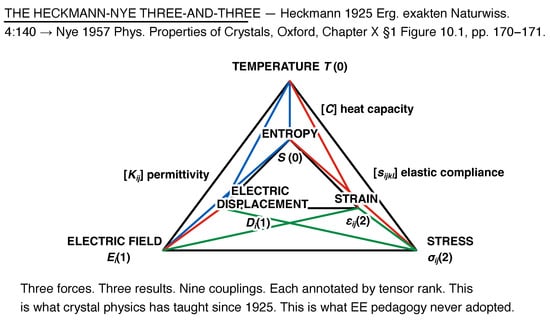
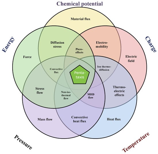
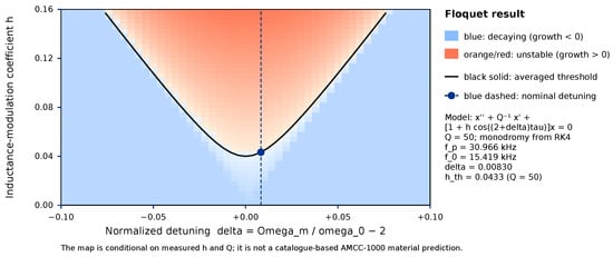
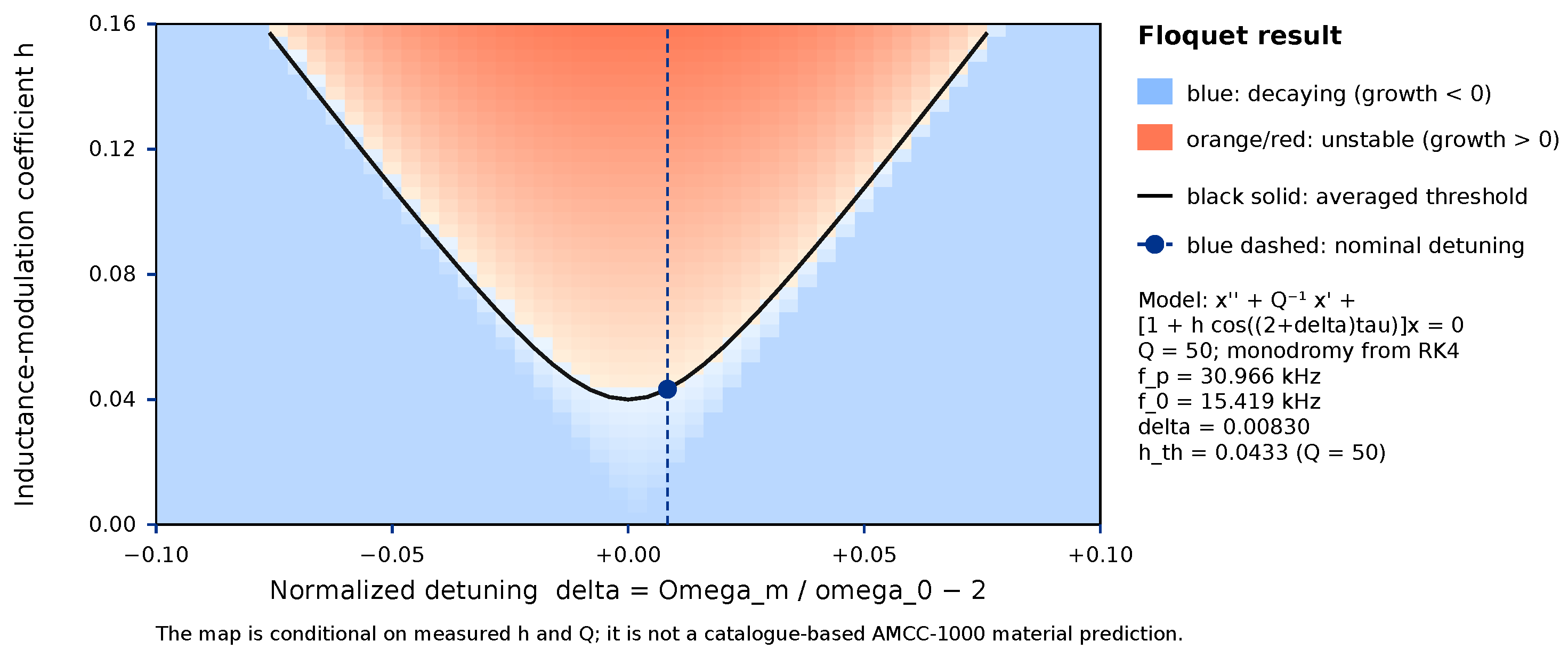
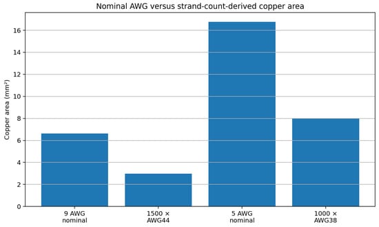
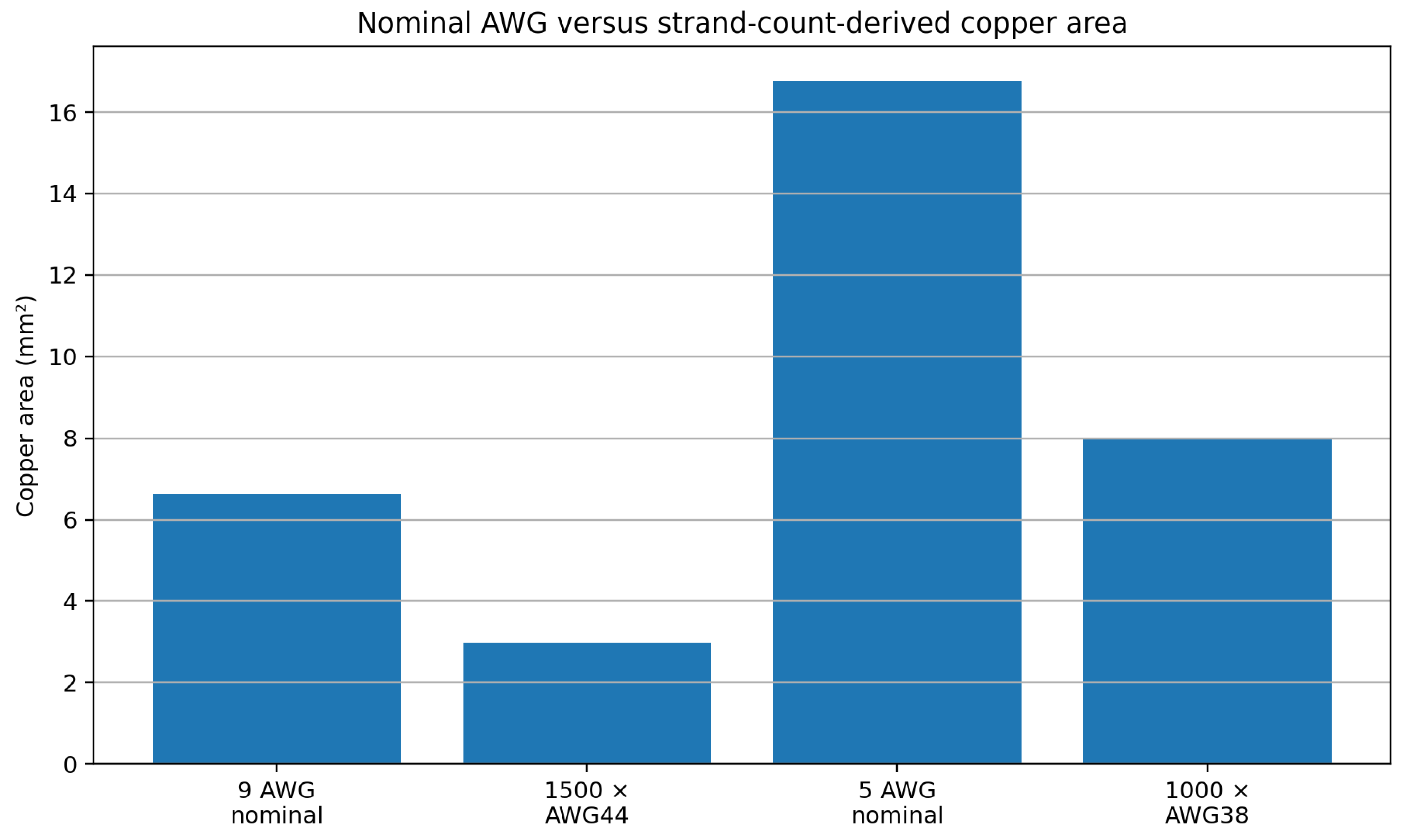
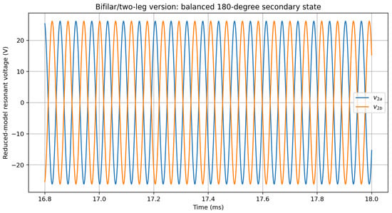
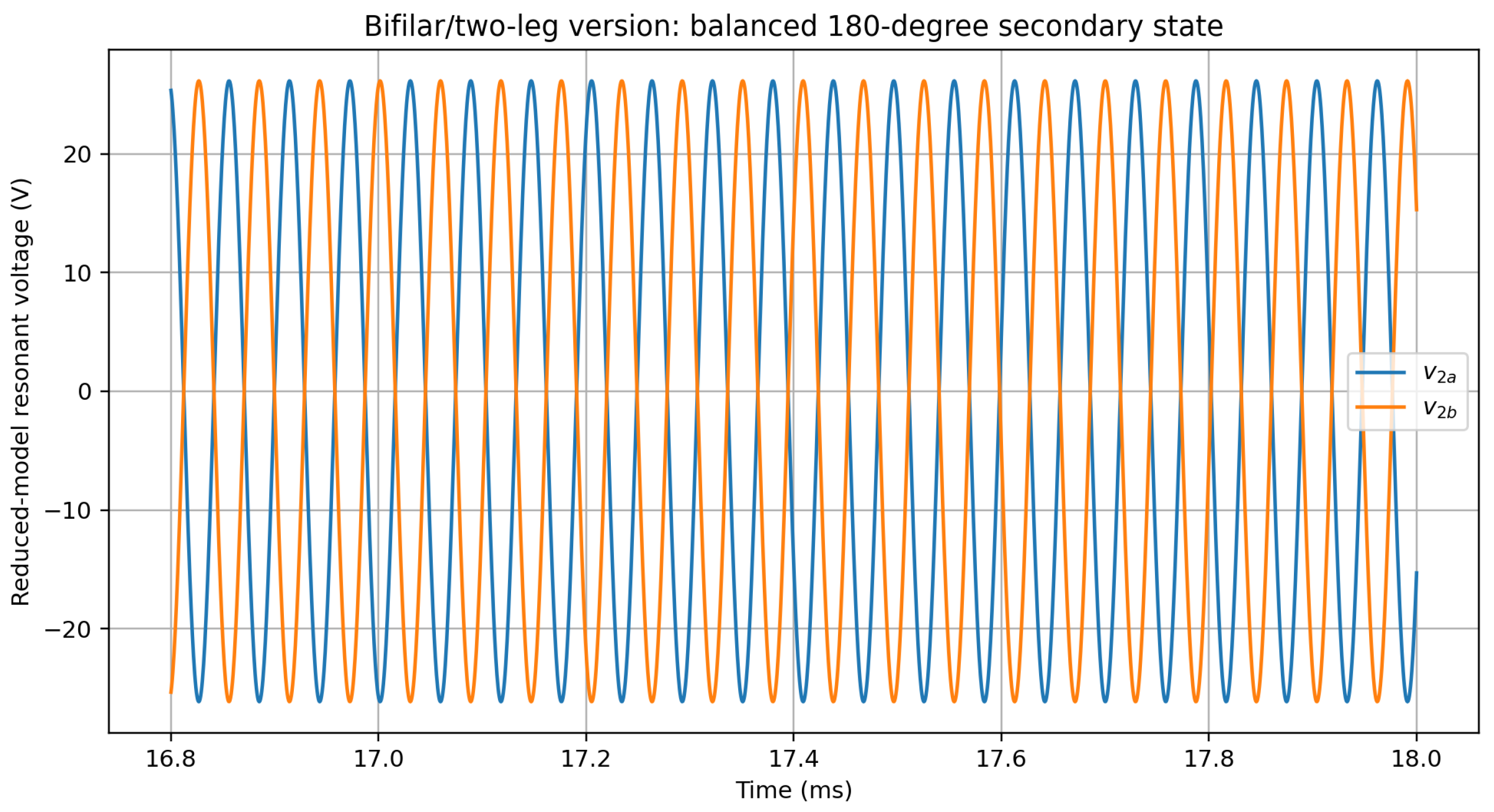
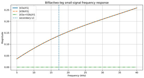
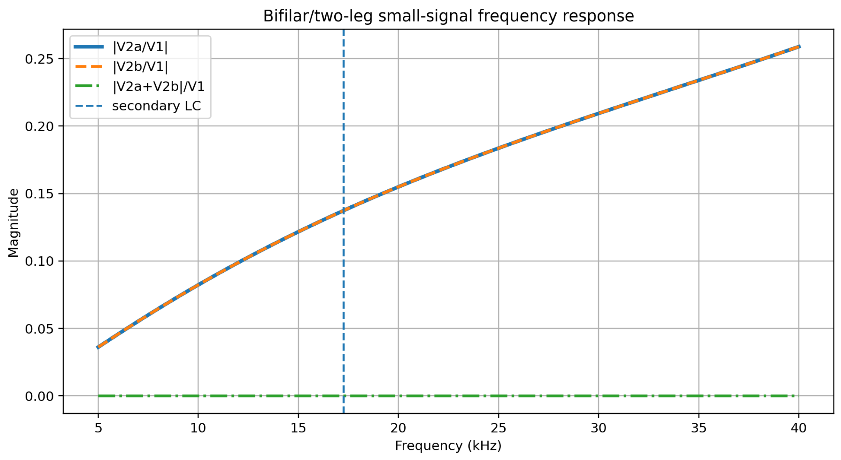
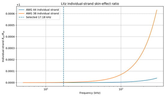
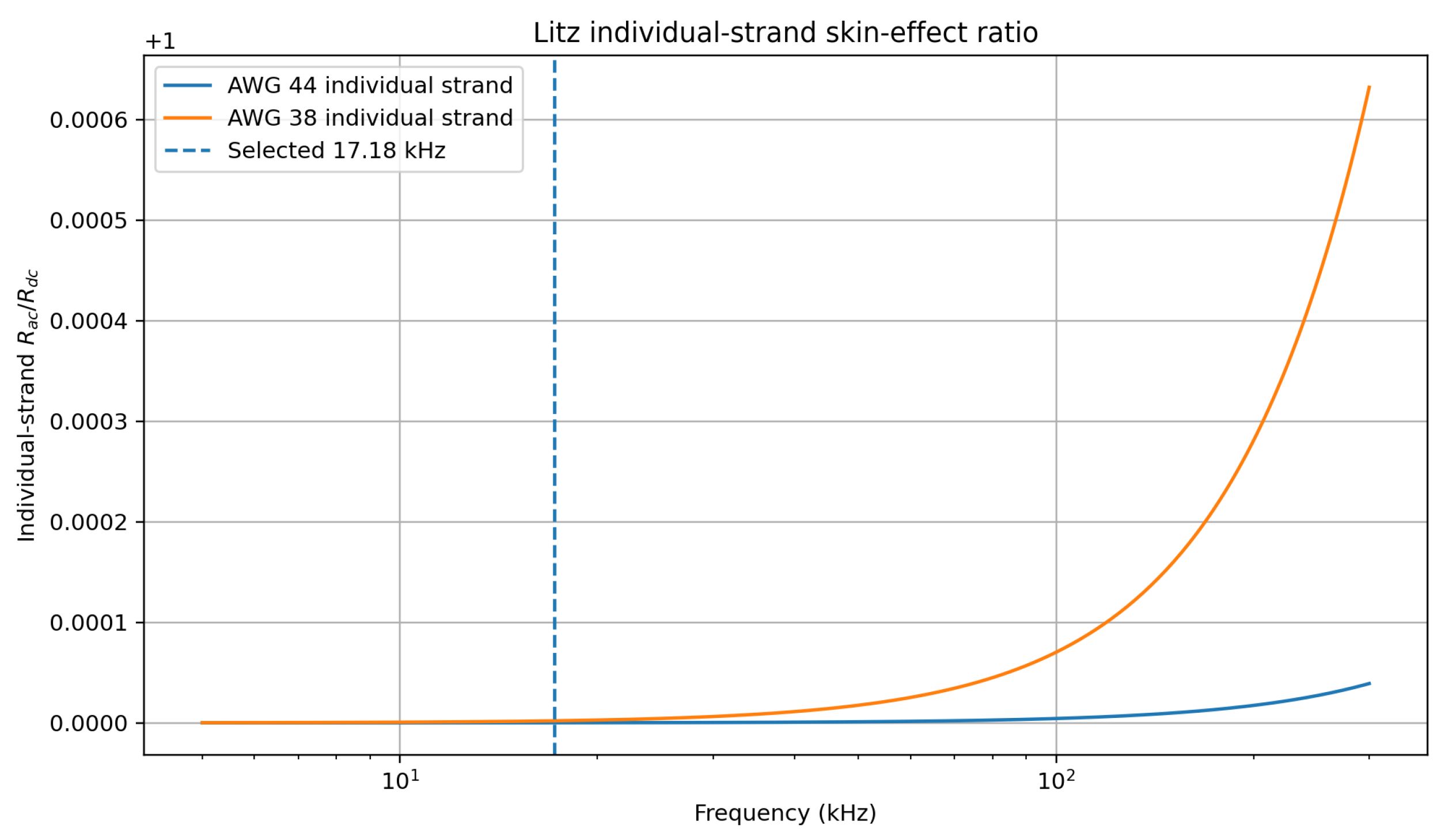
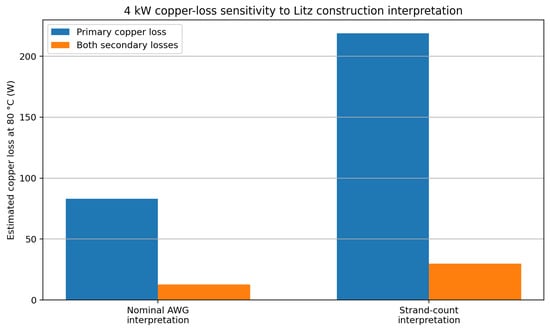
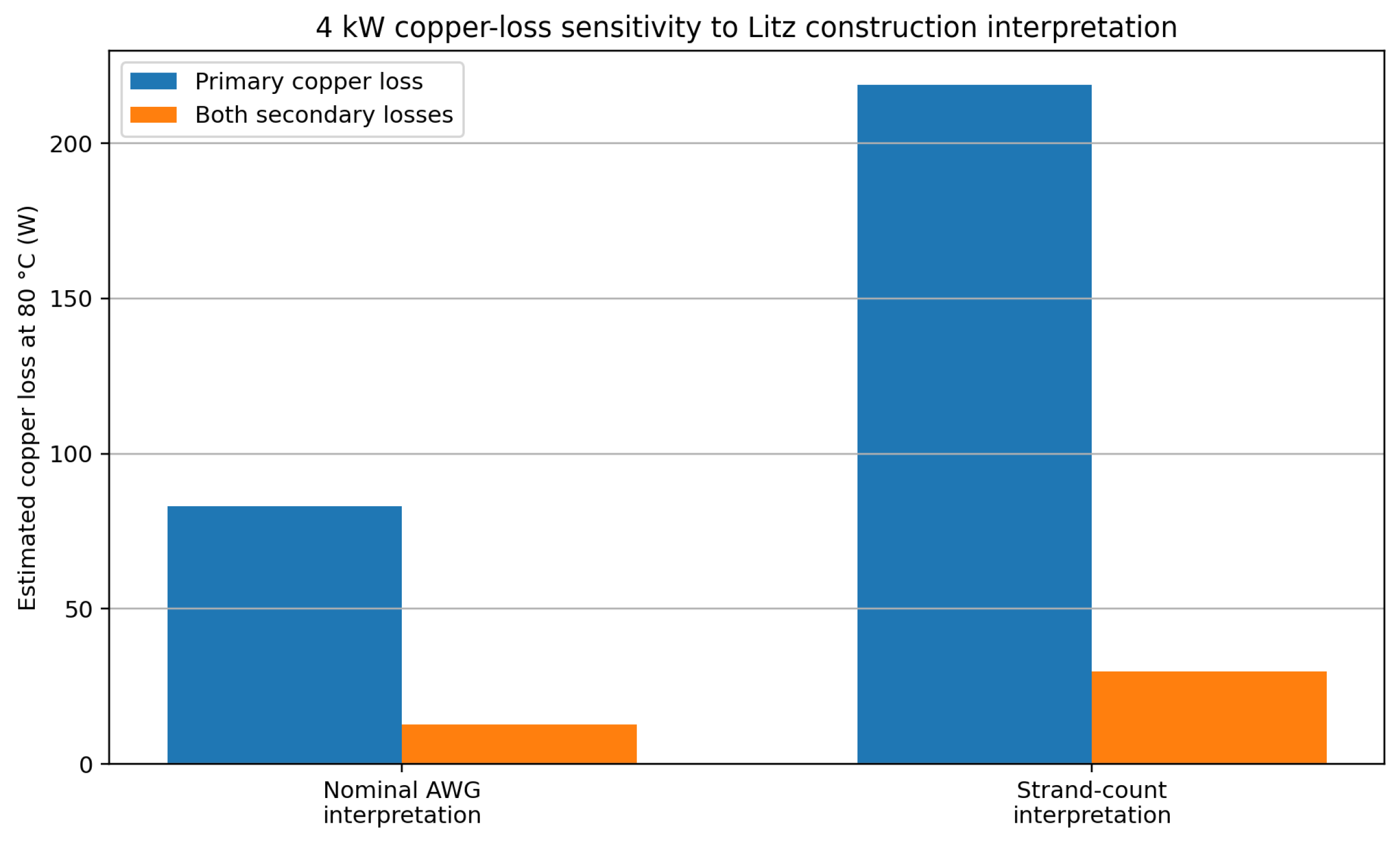
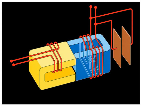
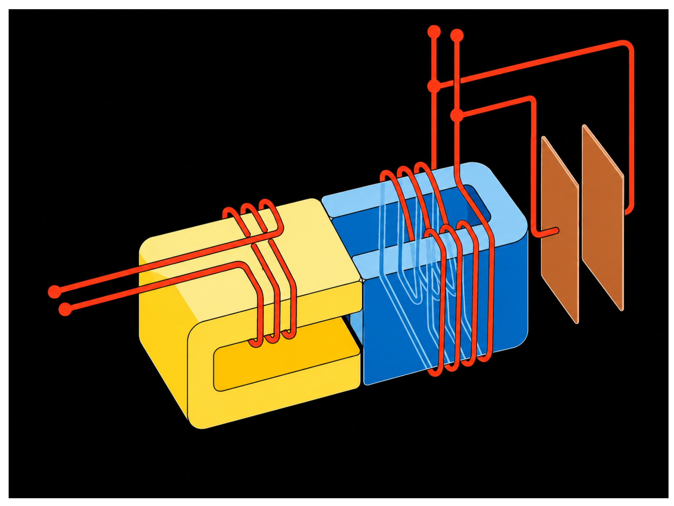
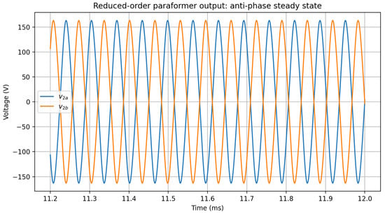
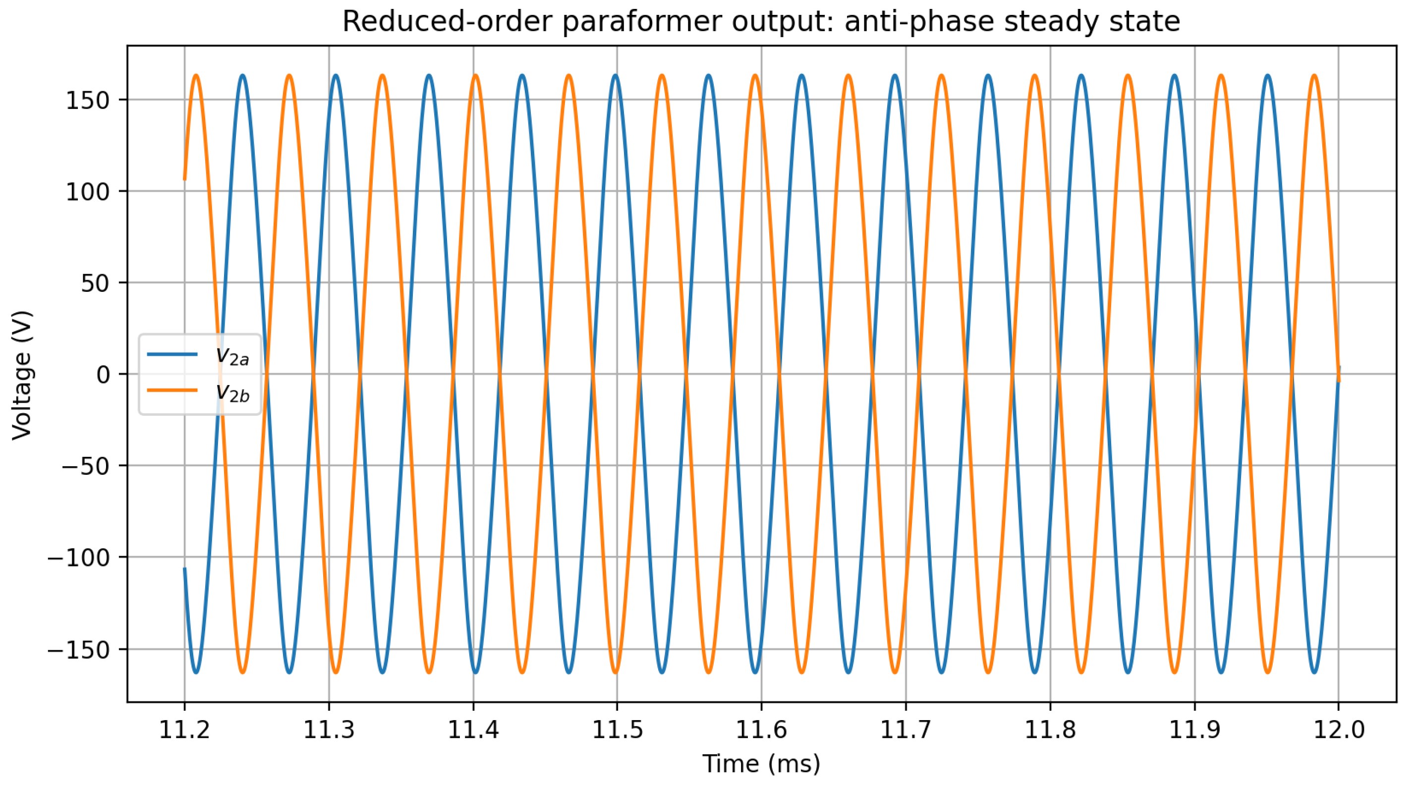
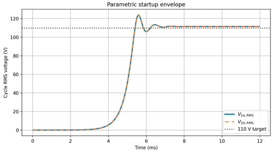
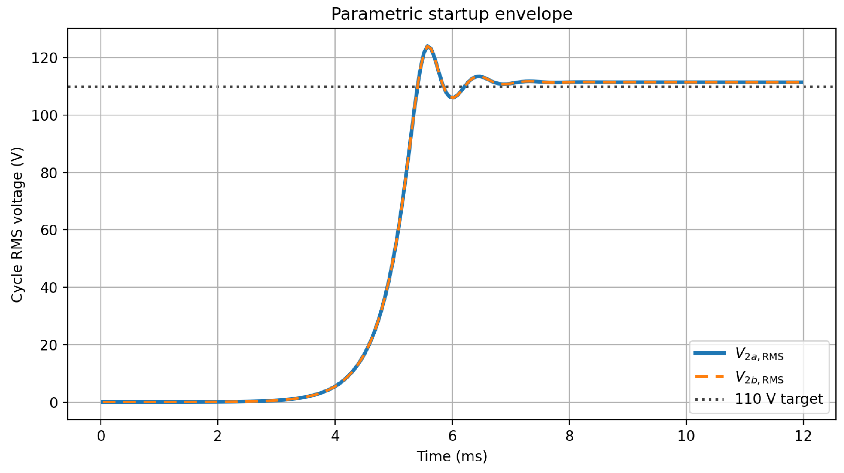
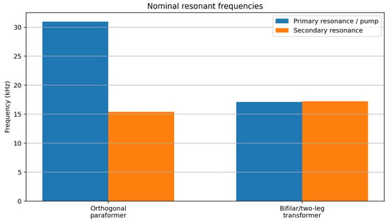
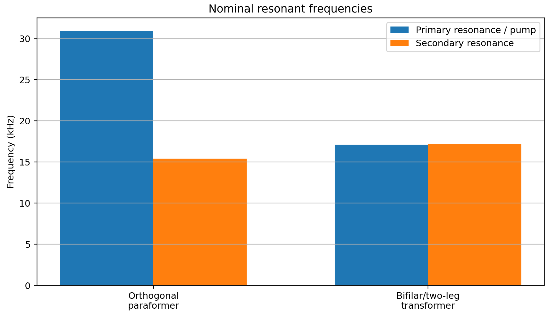
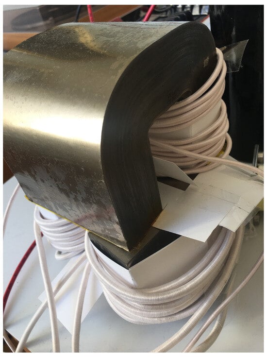
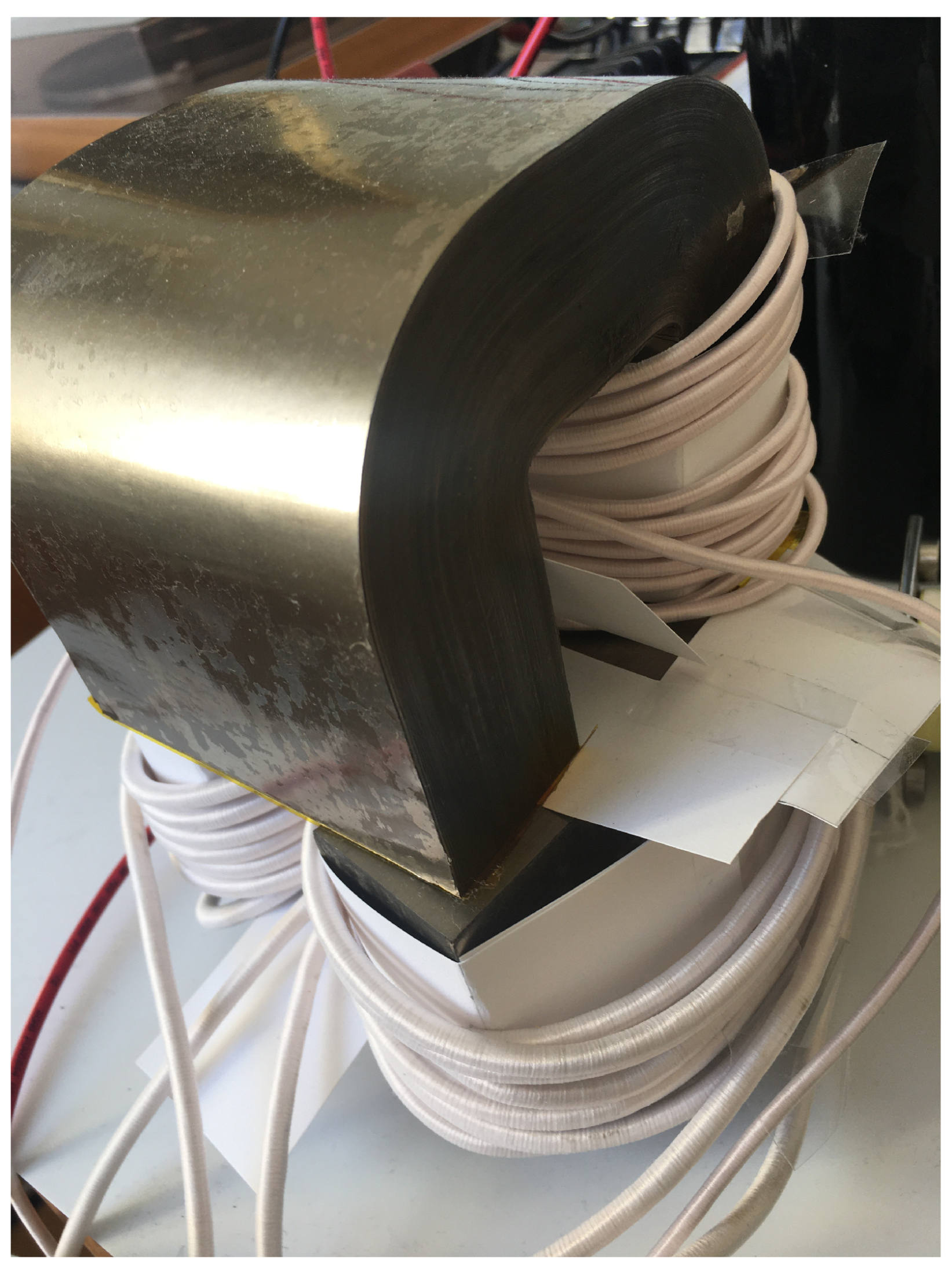
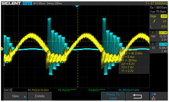
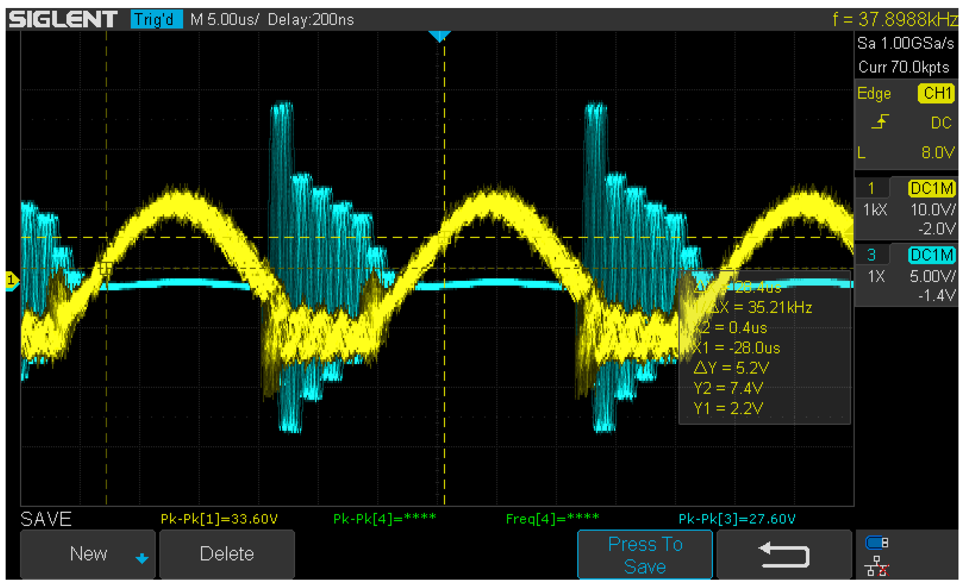

Disclaimer/Publisher’s Note: The statements, opinions and data contained in all publications are solely those of the individual author(s) and contributor(s) and not of MDPI and/or the editor(s). MDPI and/or the editor(s) disclaim responsibility for any injury to people or property resulting from any ideas, methods, instructions or products referred to in the content. |
© 2026 by the authors. Licensee MDPI, Basel, Switzerland. This article is an open access article distributed under the terms and conditions of the Creative Commons Attribution (CC BY) license.