Parametric Study of Yields and Properties of Corn Stover-Derived Hydrothermal Liquefaction Products by Using Statistical Approaches

Abstract

Hydrothermal liquefaction (HTL) of lignocellulosic biomass produces multiple product fractions, including solid residue (SR), heavy bio-oil (HBO), aqueous phase (AP), and light bio-oil (LBO). This study mainly applied principal component analysis (PCA) and regression modeling to predict AP solution weight, LBO weight and fuel characteristics, and HTL wastewater biodegradability, as well as to improve prediction accuracy for SR and HBO under various operating conditions (temperature: 250–350 °C, residence time: 5–60 min, and the combined solid loading of three batches: 15–45 g). A complementary relationship between SR and AP weights found in PCA enabled the estimation of AP weight based on predicted SR values in a regression analysis. A modified partition coefficient was introduced to link LBO weight with the carbon content of AP and was predicted, enabling accurate LBO yield estimation. Although LBO fuel characteristics could not be modeled reliably, those of SR and HBO were predicted with improved accuracy over prior kinetic models. The concentration of catechol in HTL wastewater (HTL-WW) was also modeled from operating conditions and linked to half-maximal inhibitory concentration (IC₅₀) of R. jostii and A. niger as a biodegradability index. This work demonstrates the feasibility of predicting underrepresented HTL outputs using statistical approaches.

1. Introduction

Hydrothermal liquefaction (HTL) is a promising approach for converting wet biomass into biocrude. The process is carried out by heating biomass and water in a pressure vessel under high temperature and pressure. Unlike pyrolysis, which requires dry feedstock, HTL can process wet biomass without a drying step, which is one of its major advantages. HTL generally produces three distinct phases: solid residue (SR), aqueous phase (AP), and heavy bio-oil (HBO) (also referred to as biocrude). The AP is rich in soluble organic matter, which offers potential as an organic resource; however, it also poses a drawback due to its possible toxicity to microbes [1]. Several promising treatment strategies for AP have been proposed, including biological wastewater treatment, struvite precipitation, and catalytic hydrothermal gasification, as summarized in the literature [2]. For instance, fed-batch fermentation of a high-biomass strain of Thraustochytrium striatum with 3,4-dihydroxybenzoic acid, an aromatic compound commonly found in natural lignin, increased the total fatty acid content to 22% on a dry cell weight basis [3]. Another approach is to recover organic matter in the form of oil from the aqueous phase. For example, Karagöz et al. [4] conducted a two-stage extraction using diethyl ether and ethyl acetate on the aqueous phase obtained from HTL of pinewood with bases, followed by acidification to pH 1–2, which yielded substantial amounts of oil, approaching the yield obtained from the solid phase using acetone. Similarly, Akalın et al. [5] reported the recovery of oil using diethyl ether from the AP derived from HTL of cornelian cherry stones, containing compounds such as furfurals, phenols, acetic acid, and vanillin. These examples demonstrate the potential for recovering valuable organics from AP. Research on the prediction of HTL products based on kinetic models is still active. For instance, the aqueous phase produced from the HTL of macroalgae was predicted with an accuracy where 84% of the dataset fell within the 95% prediction interval [6]. In our previous work, we predicted the yields and characteristics of SR, AP, and HBO produced from HTL of corn stover using an element-based kinetic model [7]. Light bio-oil (LBO), defined here as the oil fraction extracted from the AP as described above, is not directly associated with the kinetic model and was therefore not predicted in the previous study. However, LBO could potentially be predicted if an appropriate conversion equation relating to its extraction from AP can be established. Aside from the examples mentioned above, studies focusing on LBO recovery from AP are limited, and to the best of our knowledge, no research has addressed its prediction. The amount of AP solution is also not directly predicted by the kinetic model, but it could potentially be estimated if it is appropriately linked to model-predicted variables. Even if LBO is recovered, HTL wastewater (HTL-WW), which is defined here as the remaining aqueous phase after liquid–liquid extraction with water-insoluble organic solvents, still contains organic matter and requires biological treatment. Ideally, the biodegradability of HTL-WW should be predictable from HTL operating conditions. Once such a prediction model is established, it enables the simultaneous simulation of HTL-WW biodegradability as well as the yields and characteristics of HBO, SR, and LBO, thereby supporting the optimization of operating conditions with consideration for HTL-WW treatability. To enable such predictions, this study employed statistical methods such as principal component analysis (PCA) and regression analysis. These statistical approaches are particularly useful when constructing models for systems that lack a well-established scientific or engineering foundation.

Recently, there has been a significant increase in studies utilizing machine learning (ML) for the prediction or correlation of the yield and characteristics of the HTL or pyrolysis products. ML has demonstrated its capability to provide highly accurate predictions for the yields and properties of bioproducts [8,9,10]. For instance, Li et al. employed random forest and support vector regression (SVR) techniques to predict output parameters such as the yield and higher heating value (HHV) of hydrochar (HC) and pyrochar, based on feedstock input data including ultimate and proximate analyses [11]. They achieved average coefficients of determination of 0.90 and 0.94 for HC and pyrochar properties, respectively. While partial dependence plots (PDPs) and SHAP values can elucidate the contribution of input variables in ML models, these models lack explicit mathematical equations to represent the functional relationships between operating conditions and bioproduct outcomes. Subramanya et al. established that while the random forest model achieves the highest accuracy in predicting oil composition, multivariate linear regression is crucial for process understanding. They concluded that conventional regression models remain highly effective for chemical insights, as evidenced by their identification of novel ternary interactions between lipids, lignin, and proteins [12]. Even with the high accuracy of ML predictions, it remains essential to establish equations or functions that illustrate these relationships. Such formulations can deepen our understanding of the mechanisms involved in HTL processes and enhance the quality of scientific discussion, while supporting the practical engineering of HTL processes.

This study aims to predict the yields and characteristics of corn stover HTL products that were not be addressed in our previous research by our previous kinetic model. To begin, we explored the relationships among key variables using PCA. Based on insights from the PCA results, the AP weight was associated with SR weight. The introduced modified partition coefficient (D_mod) related the total organic carbon (TOC) in the AP to the LBO weight, and this coefficient was predicted using a regression model with operating parameters including temperature (Temp), residence time (RT), and solid loading (SL). The fuel characteristics of LBO were subsequently predicted through regression analysis based on the same operating variables. The present work aimed for more accurate estimations than our previous work by integrating PCA with regression analysis. Furthermore, the catechol concentration in HTL wastewater (HTL-WW) was predicted from operating condition, leading to a model predicting the HTL-WW biodegradability during aerobic fermentation by Aspergillus niger (A. niger) and Rhodococcus jostii (R. jostii). Finally, the study discusses the applicability and limitations of statistical models in this context.

2. Materials and Methods

2.1. Materials

Most of the materials, such as corn stover, deionized water, and paper filters, were identical to those described in our previous study [7]. In addition, dichloromethane (DCM, ≥99.8%, containing 40–150 ppm amylene as stabilizer, (Sigma-Aldrich, St. Louis, MO, USA)) was used for extracting LBO from AP.

2.2. Experimental Procedures

The experimental procedures, including HTL treatment, separation, extraction, analysis with total organic carbon (TOC), total nitrogen (TN), ash content and elemental analysis, followed those described in our previous study [7]. In the present work, a subset of the previously obtained data (the weights and elemental compositions (C, H, N, O) of SR alongside the TOC and TN in AP) was reused for further analysis. Additionally, new LBO extractions were conducted, which is not included in the prior publication. The combined AP was mixed with 225 mL of DCM in a 1000 mL separatory funnel and shaken for 10 min to extract organic compounds. After allowing the mixture to settle for phase separation, the aqueous and organic phases were carefully collected into a beaker. The aqueous phase remaining after DCM extraction is referred to as HTL-WW.

HTL-WW was analyzed with a gas chromatography–mass spectrometry (GC-MS) based on the method reported by Liu et al. [13]. The analysis was performed using an Agilent GC 6890 coupled with an MS 5973 system (Agilent Technologies, Santa Clara, CA, USA) equipped with a Zebron ZB-1701 column (30 m × 0.25 mm × 0.25 μm) (Phenomenex, Torrance, CA, USA). Helium was used as the carrier gas at a flow rate of 0.5 mL·min⁻¹. The half-maximal inhibitory concentration (IC₅₀) assay followed a previously described procedure [14].

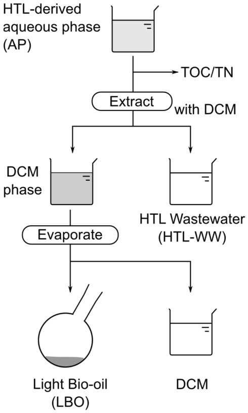
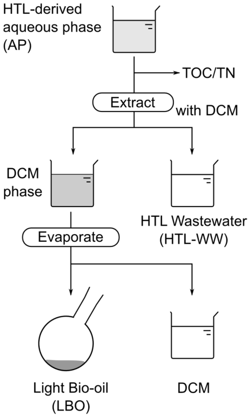
The collected DCM phase was transferred to a pre-weighed boiling flask and evaporated at 60 °C for 30 min using a rotary evaporator. After evaporation, the flask was heated in an oven at 105 °C for 30 min. It was then cooled to room temperature under ambient conditions and subsequently weighed. The viscous oil obtained from the DCM phase is referred to as LBO. The scheme for separating or collecting of LBO and HTL-WW is described in Figure 1.

Figure 1. Schematic of the HTL product separation process.

2.3. Data Analysis

Data analysis was performed using MATLAB^® (R2024b).

The root mean squared error (RMSE) and combined RMSE (RMSE₂) were used to quantify the differences between the observed and predicted data as defined in Equations (1) and (2).

$$RMSE=\sqrt{{\displaystyle \frac{1}{n}}{\displaystyle \sum _{i=1}^n}(y_i-{\widehat{y}}_i{)}^2}$$

(1)

$${RMSE}_2=\sqrt{{\displaystyle \frac{1}{2n}}{\displaystyle \sum _{i=1}^n}\left[(y_{1,i}-{\widehat{y}}_{1,i}{)}^2+(y_{2,i}-{\widehat{y}}_{2,i}{)}^2\right]}$$

(2)

For PCA, 23 variables related to HTL processing conditions and product characteristics were selected as candidates. These included process parameters (temperature, residence time, solid loading, and water input), physicochemical properties of AP (solution weight, TOC, TN, pH), and elemental compositions and yields of SR, HBO, and LBO. The nth principal component is denoted as $PCn$. Prior to performing the PCA, the dataset was optimized from 23 to 18 variables to address multicollinearity (|r| ≥ 0.9). Based on the preliminary correlation analysis, several variables exhibited redundant collinearity, including SL and TOC in AP ($r=+0.91$), TOC and TN in AP ($r=+0.93$), carbon and hydrogen contents in HBO ($r=+0.93$), carbon and oxygen contents in HBO ($r=-0.99$), hydrogen and oxygen in HBO ($r=-0.94$), carbon and hydrogen contents in LBO ($r=+0.95$), carbon and oxygen contents in LBO ($r=-1.00$), and hydrogen and oxygen contents in LBO ($r=-0.96$). To prevent statistical bias and ensure the stability of the principal components, TOC in AP (AP_TOC), hydrogen content in HBO hydrogen content in HBO (HBO_H), oxygen content in HBO (HBO_O), hydrogen content in LBO (LBO_H), and oxygen content in LBO (LBO_O) were strategically removed from the original variable matrix. This revised dataset was confirmed to be suitable for PCA, aligning with the standard requirements for linearity, sampling adequacy, and the absence of critical outliers. Up to PC3, the cumulative explained variance reached 71.3%. Detailed descriptions of the assumption verifications and statistical parameters are provided in Text S1 of the Supplementary Material. The loading factor of PCA was also applied to the van Krevelen diagrams of SR and HBO separately to reduce the two atomic ratios ($O/C$ and $H/C$) into a single principal component, denoted as ${PC1}_{\mathrm{v}\mathrm{K},\mathrm{S}\mathrm{R}}$ and ${PC1}_{\mathrm{v}\mathrm{K},\mathrm{H}\mathrm{B}\mathrm{O}}$, respectively.

The partition coefficient between the organic phase and AP is not necessarily constant. Moreover, since AP contains a variety of soluble organic compounds, it is reasonable to expect that the partition coefficient depends on the HTL conditions. To account for this, a modified partition coefficient, $D_{\mathrm{m}\mathrm{o}\mathrm{d}}$, was defined to correlate the mass concentration of LBO under each condition with the carbon content of AP solutes, which represents the primary organic component in AP, as shown in Equation (3) below:

$$D_{\mathrm{mod}}={\displaystyle \frac{w_{\mathrm{LBO}}}{w_{\mathrm{AP},\mathrm{TOC}}}}\cdot {\displaystyle \frac{V_{\mathrm{AP}}}{V_{\mathrm{DCM}}}}$$

(3)

where $w_{\mathrm{L}\mathrm{B}\mathrm{O}}$, $w_{\mathrm{A}\mathrm{P},\mathrm{T}\mathrm{O}\mathrm{C}}$, $V_{\mathrm{D}\mathrm{C}\mathrm{M}}$, and $V_{\mathrm{A}\mathrm{P}}$ represent the weight of LBO (g), the carbon weight of AP (g), the volume of DCM used for extraction (=225 mL), and the volume of AP (mL), respectively. The AP volume, $V_{\mathrm{A}\mathrm{P}}$, was estimated using Equation (4):

$$V_{\mathrm{AP}}\approx {\displaystyle \frac{w_{\mathrm{AP},\mathrm{soln}}-w_{\mathrm{AP},\mathrm{TOC}}}{d_{\mathrm{water}}}}$$

(4)

where $w_{\mathrm{A}\mathrm{P},\mathrm{s}\mathrm{o}\mathrm{l}\mathrm{n}}$, $w_{\mathrm{A}\mathrm{P},\mathrm{T}\mathrm{O}\mathrm{C}}$, and $d_{\mathrm{w}\mathrm{a}\mathrm{t}\mathrm{e}\mathrm{r}}$ denote the total weight of the AP solution (g), the weight of total organic carbon in AP (g), and the density of water (approximately 1 g·mL⁻¹), respectively. The modified partition coefficient $D_{\mathrm{m}\mathrm{o}\mathrm{d}}$ was predicted through regression analysis using Temp, RT, and SL. The predicted weight of LBO ($w_{\mathrm{L}\mathrm{B}\mathrm{O}}$) was then calculated by multiplying $D_{\mathrm{m}\mathrm{o}\mathrm{d}}$ by $w_{\mathrm{A}\mathrm{P},\mathrm{T}\mathrm{O}\mathrm{C}}$, $V_{\mathrm{A}\mathrm{P}}$, and $V_{\mathrm{D}\mathrm{C}\mathrm{M}}$, as expressed in Equation (5).

$${\widehat{w}}_{\mathrm{LBO}}={\displaystyle \frac{D_{\mathrm{m}\mathrm{o}\mathrm{d}}·w_{\mathrm{AP},\mathrm{TOC}}·V_{\mathrm{DCM}}}{V_{\mathrm{AP}}}}$$

(5)

Among the predictors, TOC stands out for its rapid and straightforward measurability. Although $D_{\mathrm{m}\mathrm{o}\mathrm{d}}$ is a semi-empirical lumped parameter that differs from classical partition coefficients, it excels in that pre-extracted AP data can be directly applied to predict the LBO weight.

The half-maximal inhibitory concentration (IC₅₀) was employed as an index of biodegradability. To predict the IC₅₀ value based on the initial environment, the relationship between the catechol concentration and the resulting IC₅₀ was modeled using a 4-parameter logistic function. This model effectively captures the characteristic sigmoidal dynamics of the dose-response relationship for toxic substances; specifically, the initial plateau at lower concentrations reflects a threshold effect where microorganisms tolerate the toxicant without significant inhibition. Exceeding this threshold triggers critical cellular damage, such as cell membrane disruption or enzyme inhibition, leading to an accelerated, steep drop in microbial activity. Finally, at elevated concentrations, the curve stabilizes into a lower plateau as the system reaches maximum bio-inactivation, where further increases in dosage yield no additional inhibitory effect.

The least-square algorithm, lsqcurvefit, was utilized for nonlinear curve fitting in MATLAB^®.

3. Results and Discussion

3.1. Experimental Data

The LBO data collected are presented in Table S1 of the Supplementary Material. The details of the yield and characteristics of LBO are discussed in Section 3.3 and Section 3.4. The other experimental data were reported in our previous research [7].

3.2. PCA

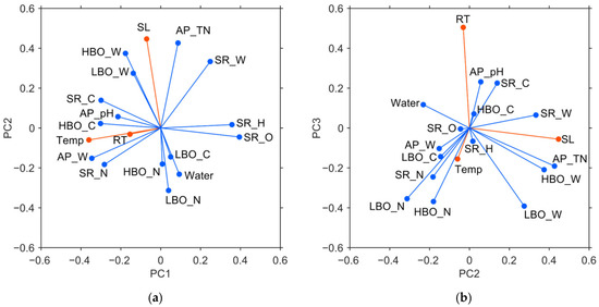
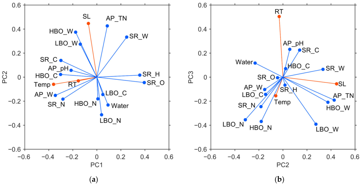
Figure 2 shows loading plots derived from PCA. The cumulative contribution ratio up to PC3 was 71.3%. It required the first five principal components to reach 87.9%. One of the key insights obtained through PCA is the relationship among variables, which can be interpreted from the loading plots. The loadings of variables are plotted in the coordinate plane or space consisting of axes of principal components obtained. Variables close to each other on the loading plot are positively correlated.

Figure 2. Loading plots from PCA of variables used. (a) PC1 vs. PC2 (b) PC2 vs. PC3. Red markers indicate main controllable variables. C, H, N, O correspond to carbon, hydrogen, nitrogen, and oxygen composition in fraction, and W denotes respective product mass. Data from our previous work [5], used under CC BY 4.0.

As shown in Figure 2a, Temp exhibited a moderate negative loading of −0.36 on PC1, indicating its substantial contribution to this component. The hydrogen and carbon ratios in HBO were also in negative side of PC1 although its oxygen content was in the positive side. Based on HHV estimation formula expressed in $HHV \left(\mathrm{MJ}/\mathrm{kg}\right)=0.335\left(\mathrm{C}\%\right)+1.423\left(\mathrm{H}\%\right)-0.154\left(\mathrm{O}\%\right)-0.145\left(\mathrm{N}\%\right)$ [15], the hydrogen and carbon contents positively affect the HHV of a bioproduct fraction whereas oxygen ratio negatively contributes to HHV. These suggest that PC1 may reflect an inverse HBO HHV component, negatively correlated with temperature. Interestingly, AP solution weight (AP_W) loaded similarly to Temp, rather than water input (Water). The SL, with a loading value of 0.45, along with TOC and TN in the AP solution (AP_TOC and AP_TN), was strongly loaded in the positive direction of PC2 on the loading plot. This layout implies that PC2 represents the indices related to SL. As shown in Figure 2b, RT exhibited high loading scores on PC3 (0.50). The AP solution weight was positioned on the opposite side of the SR weight, indicating that there was a negative correlation between them. The relationship is discussed in the following section in detail.

3.3. Relationship Between SR Weight and AP Solution Weight

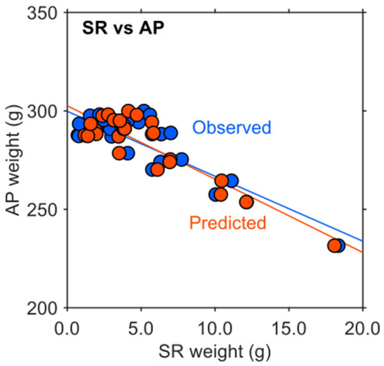
Figure 3 depicts the relationship between SR weight and AP solution weight. The blue markers represent the observed data. The regression line was descending, and AP solution weight was reduced with increasing SR weight. SR weight was negatively correlated with AP weight ($r=-0.854$). Therefore, the more SR there was, the more AP was absorbed, resulting in smaller AP solution left. As a result of the regression analysis, the following equation was derived:

$${\widehat{y}}_{\mathrm{A}\mathrm{P}\_\mathrm{W}}=299.79-3.30x_{\mathrm{S}\mathrm{R}\_\mathrm{W}}$$

(6)

where $x_{\mathrm{S}\mathrm{R}\_\mathrm{W}}$ and ${\widehat{y}}_{\mathrm{A}\mathrm{P}\_\mathrm{W}}$ correspond to the observed SR weight and predicted AP solution weight, respectively (RMSE = 8.20). This negative correlation was caused by the fact that AP solution was absorbed with SR.

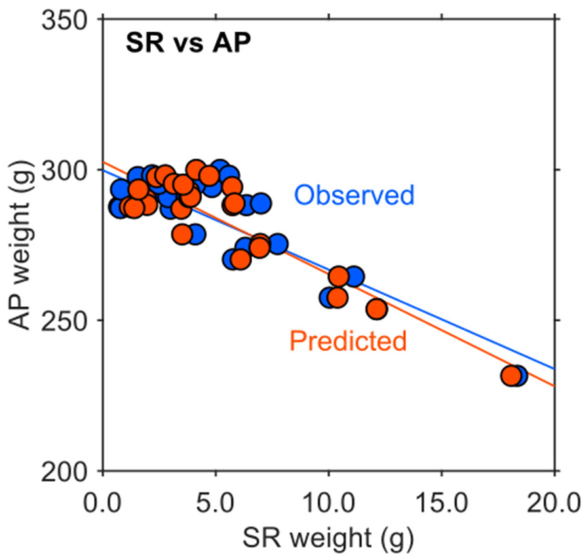
Figure 3. The relationship between SR weight and AP weight. Blue and red markers represent observed and predicted data. Data from our previous work [5], used under CC BY 4.0.

In the previous research, SR weights were well-predicted using the element-based kinetic model (RMSE = 0.73 g) [7]. The predicted SR weight data are overwrapped to the same figure using red markers. If SR weight is well-predicted, this should well-predict the corresponding AP weight. In fact, the regression line produced from the predicted SR weight was expressed as

$${\widehat{y}}_{\mathrm{A}\mathrm{P}\_\mathrm{W}}=302.59-3.73x_{\mathrm{S}\mathrm{R}\_\mathrm{W}\_\mathrm{p}\mathrm{r}\mathrm{e}\mathrm{d}}$$

(7)

where $x_{\mathrm{S}\mathrm{R}\_\mathrm{W}\_\mathrm{p}\mathrm{r}\mathrm{e}\mathrm{d}}$ denotes the predicted SR weight (RMSE = 7.18). Notably, the intercepts of both equations (299.79 g in Equation (6) and 302.59 g in Equation (7)) are extremely close. These values physically represent the theoretical initial weight of the AP solution when no SR is present ($x_{\mathrm{S}\mathrm{R}\_\mathrm{W}} {\mathrm{o}\mathrm{r} x}_{\mathrm{S}\mathrm{R}\_\mathrm{W}\_\mathrm{p}\mathrm{r}\mathrm{e}\mathrm{d}}=0$), demonstrating that the kinetic model accurately captures not only the consumption trend (slope) but also the initial state of the system. The regression equation can return the predicted AP weight values close to the values returned by the observed trend in the range of SR weight obtained this work. These results indicate that, although the AP solution weight is not directly related to the chemical reactions, it was appropriately predicted via its relationship with SR weight using an element-based kinetic model.

3.4. Modified Partition Coefficient and LBO Weight

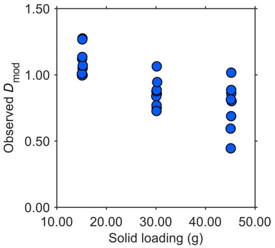
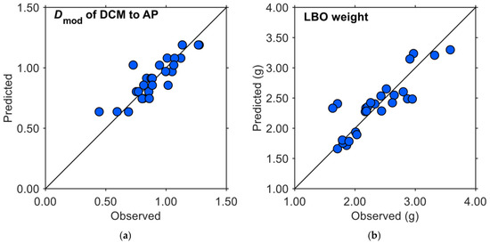
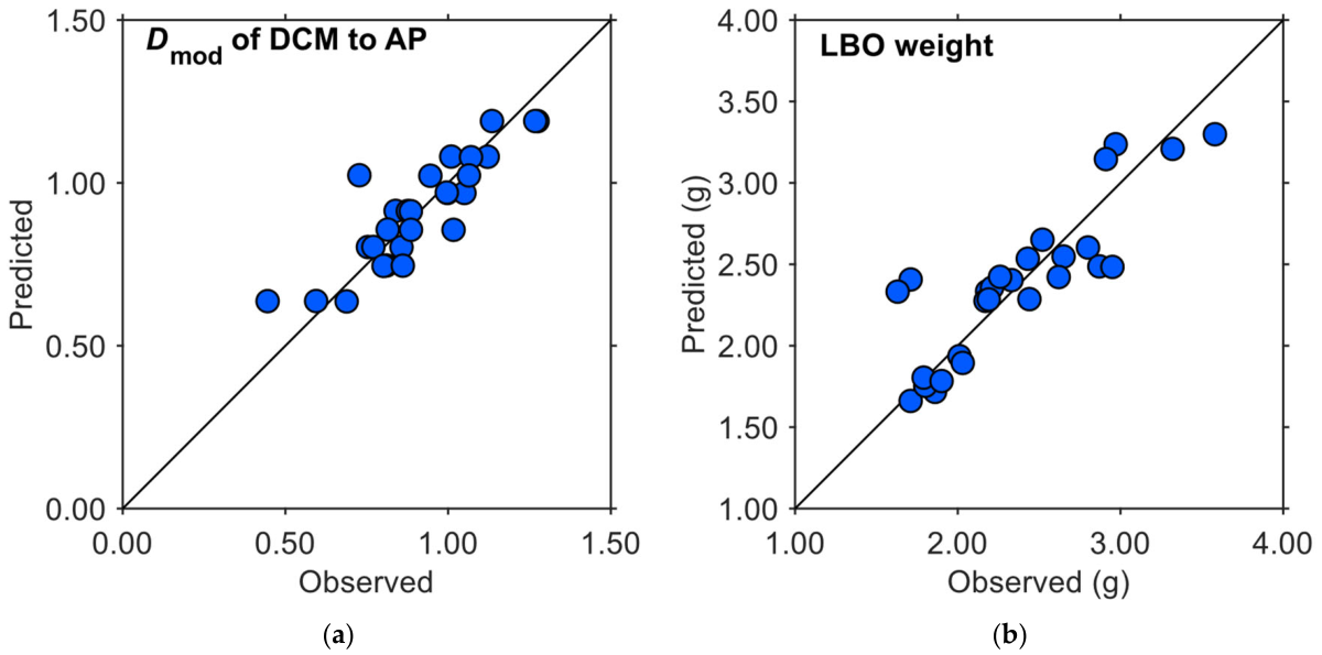
Table 1 showed the results of the regression analysis. This indicated that, with a 95% level of confidence, there was insufficient evidence to conclude that the general linear model was invalid. Looking at the validity of each variable, Temp and SL were significant variables for the linear regression model. On the other hand, RT was not a significant variable. As indicated by the F values, solid loading had the strongest effect on $D_{\mathrm{mod}}$. The regression equation for ${\widehat{D}}_{\mathrm{mod}}$, derived from the model, is as follows:

$${\widehat{D}}_{\mathrm{m}\mathrm{o}\mathrm{d}}=0.588+2.20\times {10}^{-3}{x}_{\mathrm{T}\mathrm{e}\mathrm{m}\mathrm{p}}-1.11\times {10}^{-2}{x}_{\mathrm{S}\mathrm{L}}$$

(8)

where $x_{\mathrm{T}\mathrm{e}\mathrm{m}\mathrm{p}}$, and $x_{\mathrm{S}\mathrm{L}}$ refer to temperature (°C), and total solid loading (g). Interestingly, the estimated coefficient of SL was negative. The association between the SL and observed $D_{\mathrm{mod}}$ is depicted in Figure 4. The significant and negative effect of SL weight on $D_{\mathrm{mod}}$ can be illustrated by the amount of SR obtained. Since more SR obtained took up more AP, the volume of AP remained was reduced, resulting in reducing the amount of AP solute which can be LBO. Figure 5a is the parity plot of predicted (${\widehat{D}}_{\mathrm{mod}}$) and observed ($D_{\mathrm{mod}}$), demonstrating that the predicted well fit the observed data (RMSE = 0.0925). Figure 5b is the parity plot of predicted LBO weight, calculated by Equation (5) and ${\widehat{D}}_{\mathrm{mod}}$, and observed LBO weight. The resulting relationship between the predicted LBO weight was associated with the observed value (RMSE = 0.2625 g). This statistical approach via the predicted ${\widehat{D}}_{\mathrm{mod}}$ successfully was associated with LBO weight with AP carbon weight based on Equation (5). However, it should be noted that the current calibration and evaluation were conducted using the same dataset. Therefore, these predictive performances should be interpreted cautiously as they might be optimistic.

Table 1. ANOVA table of ${\widehat{D}}_{\mathrm{mod}}$.

Source	DF	SS	MS	F Value	p Value
Regression	3	0.7180	0.2394	23.88	<0.0001
Residual	23	0.2306	0.0100	-	-
Total	26	0.9487	-	-	-
Variable	DF	Type I SS	Coefficient	95% CI	p value
Temp	1	0.2180	2.20 × 10−3	[1.22 × 10−3, 3.18 × 10−3]	0.0001
RT	1	0.0002	−1.14 × 10−4	[−1.89 × 10−3, 1.66 × 10−3]	0.8950
SL	1	0.5005	−1.11 × 10−2	[−1.44 × 10−2, −0.79 × 10−2]	<0.0001

Model summary: $R^2=0.757, Adjusted R^2=0.725$. DF, SS, MS, and CI denote degrees of freedom, sum of squares, mean square, and confidence interval, respectively. Temp, RT, and SL refer to temperature (°C), residence time (min), and solid loading (g).

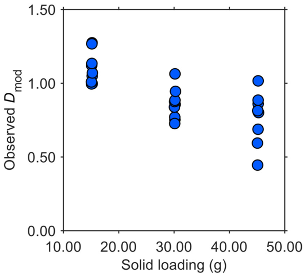
Figure 4. Scatter plot between solid loading and observed $D_{\mathrm{m}\mathrm{o}\mathrm{d}}$.

Figure 5. Prediction of LBO weight via modified partition coefficient (a) parity plot of modified partition coefficient (b) parity plot of LBO weight. Data from our previous work [5], used under CC BY 4.0.

3.5. Characteristics of LBO

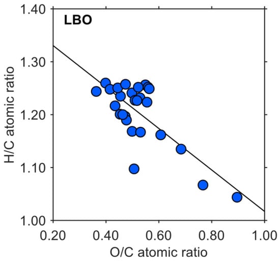
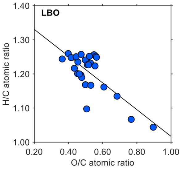
The van Krevelen diagram ($H/C$ vs. $O/C$ atomic ratio) of LBO was shown in Figure 6. The observed data of LBO were plotted with blue markers. The $O/C$ ratios ranged from 0.36 to 0.90, and the $H/C$ ratios ranged from 1.04 to 1.26. the observed data of LBO aligned in downward trend. Taking advantage of their linear layout, the first principal component (${PC1}_{\mathrm{v}\mathrm{K},\mathrm{L}\mathrm{B}\mathrm{O}}$) was produced from the variables of $H/C$ and $O/C$ to try to predict the observed data from values of Temp, RT, and SL. ${PC1}_{\mathrm{v}\mathrm{K},\mathrm{L}\mathrm{B}\mathrm{O}}$ here can be characterized as the index of occupation of carbon and hydrogen in LBO (low-rich in hydrogen, high-rich in oxygen), allowing for handling both $H/C$ and $O/C$ as an index. The regression analysis for ${PC1}_{\mathrm{v}\mathrm{K},\mathrm{L}\mathrm{B}\mathrm{O}}$ resulted in the fact that the p value of the linear regression model was 0.9. This means that, with a 95% level of confidence, there was sufficient evidence indicating that all coefficients of variables in the model to estimate ${PC1}_{\mathrm{v}\mathrm{K},\mathrm{L}\mathrm{B}\mathrm{O}}$ was zero. Therefore, the linear regression model produced did not help to predict the fuel characteristics of LBO. This lack of statistical significance can be attributed to several critical factors underlying the chemical complexity of the hydrothermal products. First, the highly complex, multi-component nature of LBO introduces substantial molecular noise, which likely masked clear statistical correlations between the macro-scale process parameters and the overall elemental ratios. Second, although the solvent used for liquid–liquid extraction remained identical across all experimental runs, the chemical composition of the resulting LBO is highly sensitive to the upstream HTL operating conditions. Variations in reaction temperature and time can induce distinct, competing pathways for molecular cracking and repolymerization, leading to structural shifts in the organic matrix that cannot be captured by a simple macro-scale regression. Furthermore, the underlying physicochemical interactions between the elemental composition and the fuel characteristics may be inherently nonlinear, falling outside the scope of the linear regression method applied in this study. Consequently, a more advanced modeling approach that accounts for these chemical complexities and nonlinearities will be required in future studies.

Figure 6. van Krevelen diagram of LBO.

3.6. Characteristics of SR and HBO

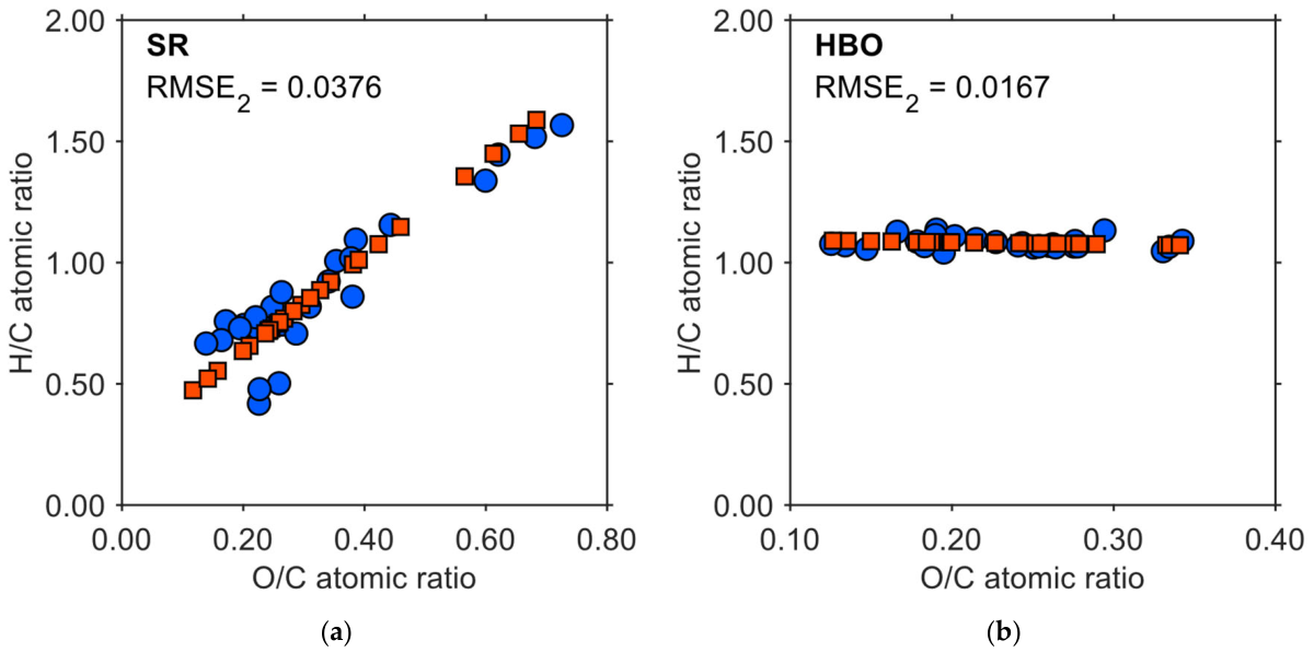
The previous work tried to associate the fuel characteristics of SR and HBO with the carbon, hydrogen, and oxygen atomic ratio predicted by element-based kinetic model, resulting in the limited accuracy of the prediction which yielded the similar trend line between the observed and predicted data [7]. Similar to the LBO as mentioned in the previous article, the fuel characteristics of SR and HBO were predicted via the first principal components of SR (${PC1}_{\mathrm{v}\mathrm{K},\mathrm{S}\mathrm{R}}$) and HBO (${PC1}_{\mathrm{v}\mathrm{K},\mathrm{H}\mathrm{B}\mathrm{O}}$) in the van Krevelen diagram. ${PC1}_{\mathrm{v}\mathrm{K},\mathrm{S}\mathrm{R}}$ and ${PC1}_{\mathrm{v}\mathrm{K},\mathrm{H}\mathrm{B}\mathrm{O}}$ produced from the observed data [7] were expressed as shown in Equations (9) and (10) below:

$${H/C}_{\mathrm{S}\mathrm{R}}=1.968·{O/C}_{\mathrm{S}\mathrm{R}}+0.243$$

(9)

$${H/C}_{\mathrm{H}\mathrm{B}\mathrm{O}}=-0.086·{O/C}_{\mathrm{H}\mathrm{B}\mathrm{O}}+1.101$$

(10)

with RMSE₂ = 0.0376 and RMSE₂ = 0.0167, respectively. The results of regression analysis for ${PC1}_{\mathrm{v}\mathrm{K},\mathrm{S}\mathrm{R}}$ and ${PC1}_{\mathrm{v}\mathrm{K},\mathrm{H}\mathrm{B}\mathrm{O}}$ are shown in Table 2 and Table 3. These tables demonstrate that, with a 95% level of confidence, there was insufficient evidence indicating that all coefficients of variables in the model to estimate ${PC1}_{\mathrm{v}\mathrm{K},\mathrm{S}\mathrm{R}}$ and ${PC1}_{\mathrm{v}\mathrm{K},\mathrm{H}\mathrm{B}\mathrm{O}}$ were zero. Therefore, the regression coefficients were found to be statistically valid, leading to the following Equations (11) and (12), respectively:

$${PC1}_{\mathrm{v}\mathrm{K},\mathrm{S}\mathrm{R}}=3.73-5.84\times {10}^{-3}{x}_{\mathrm{T}\mathrm{e}\mathrm{m}\mathrm{p}}-6.88\times {10}^{-3}{x}_{\mathrm{R}\mathrm{T}}-5.39\times {10}^{-3}{x}_{\mathrm{S}\mathrm{L}}$$

(11)

$${PC1}_{\mathrm{v}\mathrm{K},\mathrm{H}\mathrm{B}\mathrm{O}}=0.625-9.99\times {10}^{-4}{x}_{\mathrm{T}\mathrm{e}\mathrm{m}\mathrm{p}}-8.34\times {10}^{-4}{x}_{\mathrm{R}\mathrm{T}}$$

(12)

Table 2. ANOVA table of ${PC1}_{\mathrm{v}\mathrm{K},\mathrm{S}\mathrm{R}}$.

Source	DF	SS	MS	F Value	p Value
Regression	3	2.3002	0.7667	28.06	<0.0001
Residue	23	0.6284	0.0273
Total	26	2.9286
Variable	DF	Type I SS	Coefficient	95% CI	p value
Temp	1	1.5359	−5.84 × 10−3	[−7.45 × 10−3, −4.23 × 10−3]	<0.0001
RT	1	0.6467	−6.88 × 10−3	[−9.81 × 10−3, −3.96 × 10−3]	<0.0001
SL	1	0.1177	−5.39 × 10−3	[−10.76 × 10−3, 0.00 × 10−3]	0.0493

Model summary: $R^2=0.785,\mathrm{A}\mathrm{d}\mathrm{j}\mathrm{u}\mathrm{s}\mathrm{t}\mathrm{e}\mathrm{d} R^2=0.757$. DF, SS, MS, and CI denote degrees of freedom, sum of squares, mean square, and confidence interval, respectively. Temp, RT, SL refer to temperature (K), residence time (min), solid loading (g).

Table 3. ANOVA table of ${PC1}_{\mathrm{v}\mathrm{K},\mathrm{H}\mathrm{B}\mathrm{O}}$.

Source	DF	SS	MS	F Value	P Value
Regression	3	0.0574	0.0191	13.23	<0.0001
Residue	23	0.0333	0.0014
Total	26	0.0907
Variable	DF	Type I SS	Coefficient	95% CI	p value
Temp	1	0.0450	−9.99 × 10−4	[−13.70 × 10−4, −6.29 × 10−4]	<0.0001
RT	1	0.0095	−8.34 × 10−4	[−15.10 × 10−4, 1.61 × 10−4]	0.0174
SL	1	0.0029	−8.52 × 10−4	[−2.09 × 10−4, 3.84 × 10−4]	0.1672

Model summary: $R^2=0.633,\mathrm{A}\mathrm{d}\mathrm{j}\mathrm{u}\mathrm{s}\mathrm{t}\mathrm{e}\mathrm{d} R^2=0.585$. DF, SS, MS, and CI denote degrees of freedom, sum of squares, mean square, and confidence interval, respectively. Temp, RT, SL refer to temperature (K), residence time (min), solid loading (g).

By inversely projecting the PC1s onto the original van Krevelen diagram plane, the following Equations (13)–(16) were represented:

$${O/C}_{\mathrm{S}\mathrm{R}}=0.856-9.96\times {10}^{-4}{x}_{\mathrm{T}\mathrm{e}\mathrm{m}\mathrm{p}}-8.31\times {10}^{-4}{x}_{\mathrm{R}\mathrm{T}}$$

(13)

$${H/C}_{\mathrm{S}\mathrm{R}}=1.134-8.52\times {10}^{-5}{x}_{\mathrm{T}\mathrm{e}\mathrm{m}\mathrm{p}}-7.11\times {10}^{-5}{x}_{\mathrm{R}\mathrm{T}}$$

(14)

$${O/C}_{\mathrm{H}\mathrm{B}\mathrm{O}}=2.015-2.65\times {10}^{-3}{x}_{\mathrm{T}\mathrm{e}\mathrm{m}\mathrm{p}}-3.12\times {10}^{-3}{x}_{\mathrm{R}\mathrm{T}}-2.44\times {10}^{-3}{x}_{\mathrm{S}\mathrm{L}}$$

(15)

$${H/C}_{\mathrm{H}\mathrm{B}\mathrm{O}}=4.209-5.21\times {10}^{-3}{x}_{\mathrm{T}\mathrm{e}\mathrm{m}\mathrm{p}}-6.14\times {10}^{-3}{x}_{\mathrm{R}\mathrm{T}}-4.80\times {10}^{-3}{x}_{\mathrm{S}\mathrm{L}}$$

(16)

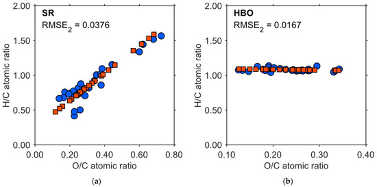
where $x_{\mathrm{T}\mathrm{e}\mathrm{m}\mathrm{p}}$ is temperature (K), $x_{\mathrm{R}\mathrm{T}}$ is residence time (min), and $x_{\mathrm{S}\mathrm{L}}$ is solid loading (g). In Figure 7, these newly predicted data were overlaid on the observed data reported previously, indicating that the prediction this time became more accurate over the prediction by the element-based kinetic model approach with RMSE₂ = 0.2093 for SR and RMSE₂ for HBO = 0.0586 for HBO [7]. Specifically, the newly developed equations yielded significantly lower RMSE₂ values of 0.0376 for SR and 0.0167 for HBO, demonstrating a substantial reduction in prediction error compared to the previous model.

Figure 7. van Krevelen diagram of SR and HBO. Blue circle and red square markers represent observed and predicted data, respectively. (a) SR (b) HBO. Modified from our previous work [7], used under CC BY 4.0.

3.7. HTL-WW Catechol Concentration and Biodegradability

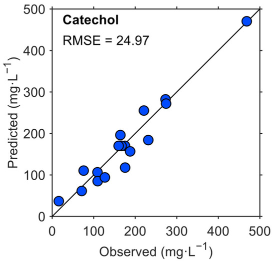
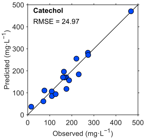
Among the carbon sources in the HTL-WW obtained from corn stover, catechol exhibited the largest peak area in the GC-MS chromatogram, which appeared to be influenced by operating conditions such as Temp, RT, and SL [14]. Therefore, it was assumed that cell inhibition was primarily influenced by the catechol concentration, serving as a representative index for predicting inhibition. In studies of HTL, the severity index, which is a concept integrating temperature and time, is frequently employed. Given that severity indices are often expressed as function such as ${\int }_0^t\mathit{e}\mathit{x}\mathit{p}\left({\displaystyle \frac{T\left(t\right)-100}{14.75}}\right)dt$ [16], $50t^{0.2}exp\left(-{\displaystyle \frac{3500}{T}}\right)$ [17], or ${\int }_0^{t}exp\left[-{\displaystyle \frac{E_b}{R}}\left({\displaystyle \frac{1}{T}}-{\displaystyle \frac{1}{T_0}}\right)\right]dt$ [18], the catechol concentrations (mg·L⁻¹) in HTL-WW in this study was assumed to be proportional to ${x_{RT}}^{C_2}$, $\mathrm{e}\mathrm{x}\mathrm{p}\left(C_3{x}_{Temp}+C_4\right)$ and $x_{SL}$. Consequently, to determine the constants $C_1$ through $C_4$, the curve fitting was conducted for a product-form equation: ${\widehat{y}}_{\mathrm{c}\mathrm{a}\mathrm{t}}=C_1{x}_{\mathrm{S}\mathrm{L}}·{x_{\mathrm{R}\mathrm{T}}}^{C_2}·exp\left(C_3{x}_{\mathrm{T}\mathrm{e}\mathrm{m}\mathrm{p}}+C_4\right)$. Here, $x_{\mathrm{S}\mathrm{L}}$, $x_{\mathrm{R}\mathrm{T}}$, and $x_{\mathrm{T}\mathrm{e}\mathrm{m}\mathrm{p}}$ refer to the values of SL (g), RT (min), and Temp (K). The predicted concentrations showed good agreement with the observed values, and the resulting equation was:

$${\widehat{y}}_{cat}=6.80\times {10}^{-6}{x}_{\mathrm{S}\mathrm{L}}·{x_{\mathrm{R}\mathrm{T}}}^{0.206}·exp\left(9.38\times {10}^{-3}{x}_{\mathrm{T}\mathrm{e}\mathrm{m}\mathrm{p}}+8.66\right)$$

(17)

with RMSE = 24.97 mg·L⁻¹. The parity plot of catechol concentration is presented in Figure 8.

Figure 8. Parity plot of catechol concentration. Modified from Ref. [14], with permission from Elsevier.

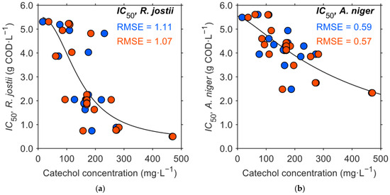
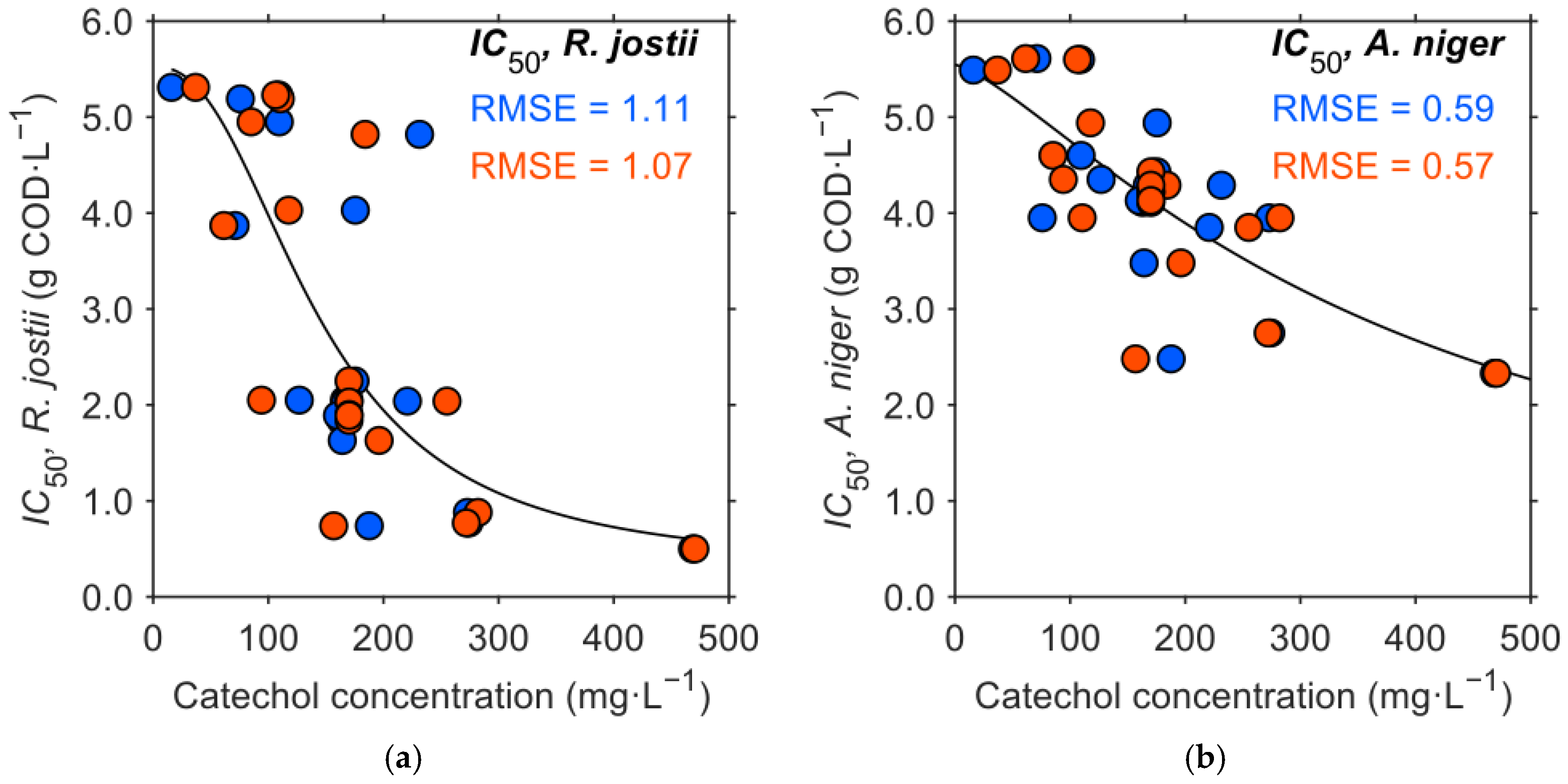
Figure 9 shows the results regarding the prediction of biodegradability of HTL-WW. The relationships between catechol concentration (mg·L⁻¹) and IC₅₀ of R. jostii and A. niger (g COD·L⁻¹) are shown in Figure 9a,b. Blue markers came from the observed catechol concentration. The plot seems to be scattered with a sigmoidal tendency, rather than a linear tendency. Therefore, the curves in the figures were thus fit by four-parameter logistic ($y_{{IC}_{50}}=d+{\displaystyle \frac{a-d}{1+{\left(\frac{x_{\mathrm{c}\mathrm{a}\mathrm{t}}}{c}\right)}^b}}$) with the observed catechol concentrations, where $y_{{IC}_{50}}$ and $x_{\mathrm{c}\mathrm{a}\mathrm{t}}$ represent IC₅₀ of each microbe (g COD·L⁻¹) and catechol concentration in HTL-WW (mg·L⁻¹), respectively. Those curves were fit to Equations (18) and (19) below:

$$y_{{IC}_{50}\_R.jostii}=0.30+{\displaystyle \frac{5.23}{1+{\left(\frac{x_{\mathrm{c}\mathrm{a}\mathrm{t}}}{143.97}\right)}^{2.37}}}$$

(18)

$$y_{{IC}_{50}\_A.niger}={\displaystyle \frac{5.55}{1+{\left(\frac{x_{\mathrm{c}\mathrm{a}\mathrm{t}}}{379.42}\right)}^{1.34}}}$$

(19)

with RMSE = 1.11 g COD·L⁻¹ for IC₅₀ of R. jostii and RMSE = 0.59 g COD·L⁻¹ for IC₅₀ of A. niger, respectively. The red markers come from the catechol concentration predicted by Temp, RT, and SL above. The red ones also appeared in the form of sigmoidal curve. The RMSEs of the predicted were 1.07 g COD·L⁻¹ for IC₅₀ of R. jostii and 0.57 g COD·L⁻¹ for that of A. niger. These results eventually indicated that the biodegradability of HTL-WW by R. jostii and A. niger can be predicted with values of Temp, RT, and SL. Catechol was selected as a practical indicator for biodegradability because it was the dominant component (the largest peak) in the GC-MS analysis. However, the toxicity of the entire system may also be influenced by minor components through complex interactions such as synergistic effects. Therefore, while monitoring catechol is an efficient tool for tracking system performance, further detailed analysis of the multi-component matrix remains a subject for future studies.

Figure 9. Prediction of biodegradability of HTL-WW. Relationship between catechol concentration and IC₅₀ of (a) R. jostii and (b) A. niger. Blue markers indicate data obtained from observed catechol concentration and red markers indicate data obtained from catechol concentration predicted by temperature, residence time, and solid loading. Solid curves represent four-parameter logistic fit for the observed catechol concentration data. Data from Ref. [14], with permission from Elsevier.

3.8. Applicability and Limitation of Prediction

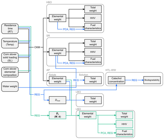
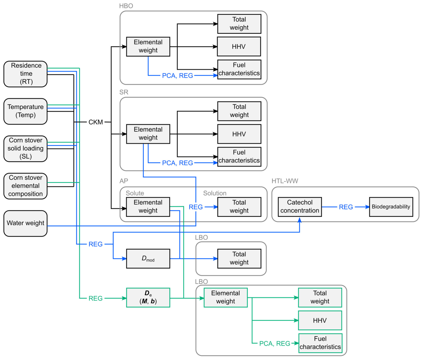
The statistical framework developed in this study provides significant engineering advancements beyond chemical kinetic models. While kinetic models are inherently limited to simulating chemical reaction pathways, the integration of PCA and regression analysis identifies and quantifies non-reactive physical phenomena, such as the physical absorption of the AP solution by the SR phase. Furthermore, this framework establishes a comprehensive, system-wide simulation that simultaneously links controllable operating variables to both downstream product recovery (LBO weight) and environmental treatability (${IC}_{50}$ biological inhibition indexes). Figure 10 illustrates relationships between independent variables (operating condition) and dependent variables (weights or characteristics of HTL products), along with the models used to develop the relationships. As described in the preceding sections, this work focused on predicting the yields and properties of HTL products, as well as biodegradability of HTL-WW, which were aspects not addressed in the previous work. By integrating these findings with the previous ones, the predictive scope encompasses the weight and characteristics of HBO and SR, the elemental weights of AP solutes (carbon and nitrogen), AP solution weight, LBO weight, and the biodegradability of HTL-WW. These parameters can assist in engineering the HTL process for corn stover in industrial applications to optimize fuel production while proactively assessing wastewater management within a unified predictive tool.

Figure 10. Schematic of relationship among operating conditions, product characteristics/yields, predictive models which have been developed by this and previous work [7]. Blue line shows relationships developed this time. Black line shows relationships developed previous work. Green line shows relationships that will be developed as futuristic work. PCA, REG, CKM denote the use of model including principal component analysis, regression analysis, element-based chemical kinetic analysis, respectively.

On the other hand, regarding the fuel characteristics of LBO, a significant predictive model could not be developed by using the combination of PCA and regression analysis, which represents a limitation of this work. To address this challenge, predicting LBO weight and characteristics via element-based partition coefficient, ${\mathit{D}}_{\mathrm{e}}$, is proposed as a future direction. ${\mathit{D}}_{\mathrm{e}}$ represents a 4 × 4 diagonal matrix defined by the equation: ${\mathit{w}}_{\mathrm{L}\mathrm{B}\mathrm{O},\mathrm{e}}={\mathit{D}}_{\mathrm{e}}{\mathit{w}}_{\mathrm{A}\mathrm{P},\mathrm{e}}$, where ${\mathit{w}}_{\mathrm{L}\mathrm{B}\mathrm{O},\mathrm{e}}$ and ${\mathit{w}}_{\mathrm{A}\mathrm{P},\mathrm{e}}$ denote vectors whose entries represent the weights of C, H, N, and O in LBO and AP after extraction, respectively, such that ${\mathit{w}}_{\mathrm{L}\mathrm{B}\mathrm{O},\mathrm{e}}={\left[w_{\mathrm{L}\mathrm{B}\mathrm{O},\mathrm{C}},w_{\mathrm{L}\mathrm{B}\mathrm{O},\mathrm{H}},w_{\mathrm{L}\mathrm{B}\mathrm{O},\mathrm{N}},w_{\mathrm{L}\mathrm{B}\mathrm{O},\mathrm{O}}\right]}^T$ and ${w_{\mathrm{A}\mathrm{P},\mathrm{e}}=\left[w_{\mathrm{A}\mathrm{P},\mathrm{C}},w_{\mathrm{A}\mathrm{P},\mathrm{H}},w_{\mathrm{A}\mathrm{P},\mathrm{N}},w_{\mathrm{A}\mathrm{P},\mathrm{O}}\right]}^T$). The matrix ${\mathit{D}}_{\mathrm{e}}$ is defined as a diagonal matrix constructed from the vector $\mathit{M}\mathit{x}+\mathit{b}$. Specifically, ${\mathit{D}}_{\mathrm{e}}=diag(\mathit{M}\mathit{x}+\mathit{b})$, where the operator “diag” denotes the transformation of the vector into the diagonal elements of a 4 × 4 matrix. Here, $\mathit{x}$ is a vector of three operating conditions ${\left[x_{\mathrm{T}\mathrm{e}\mathrm{m}\mathrm{p}},x_{\mathrm{R}\mathrm{T}},x_{\mathrm{S}\mathrm{L}}\right]}^T$, $\mathit{b}$ is a four-component residual vector, ${\left[b_{\mathrm{C}},b_{\mathrm{H}},b_{\mathrm{N}},b_{\mathrm{O}}\right]}^T$, and $\mathit{M}$ is a 4 × 3 matrix relating the elements to the operating conditions. Thus, determining $\mathit{M}$ and $\mathit{b}$ allows for the prediction of each elemental weight in LBO, ultimately enabling the estimation of LBO HHV and other fuel characteristics.

4. Conclusions

This study successfully applied statistical approaches by integrating principal component analysis (PCA) and regression modeling to enhance the predictive capabilities for hydrothermal liquefaction (HTL) of corn stover. The models were developed across a broad range of operating conditions, including temperatures of 250–350 °C, residence times of 5–60 min, and total solid loadings of 15–45 g. The primary achievement of this work was extending the predictive scope to include previously underrepresented product fractions, specifically the aqueous phase (AP) solution weight and light bio-oil (LBO) weight.

A strong negative correlation was identified between solid residue (SR) weight and AP solution weight by using PCA, enabling the accurate estimation of AP weight based on SR values. Furthermore, the introduction of a modified partition coefficient $D_{\mathrm{m}\mathrm{o}\mathrm{d}}$ allowed for the successful prediction of LBO yield (RMSE = 0.2625 g).

While LBO fuel characteristics proved challenging to model, the integration of PCA with regression analysis improved the prediction accuracy for the fuel characteristics of SR and HBO. These models outperformed prior element-based kinetic models in terms of it, with combined RMSE (RMSE₂) of 0.0376 for SR and 0.0167 for HBO.

A predictive equation for catechol concentration in HTL-WW was established as a product-form function of the operating conditions, which yielded good predictions with RMSE = 24.97 mg·L⁻¹. Subsequently, by utilizing catechol concentration as a representative inhibitory index and applying a four-parameter logistic curve, the half-maximal inhibitory concentration (IC₅₀), a biodegradability index for R. jostii and A. niger, can now be predicted directly from the initial process parameters with RMSEs of 1.07 and 0.57 g COD·L⁻¹, respectively. Ultimately, these results demonstrate that HTL operating conditions markedly influence both catechol concentration and the resulting biodegradability of HTL-WW, enabling the optimization of the process for improved wastewater treatability.

This integrated statistical framework provides a comprehensive tool for predicting HTL product yields, fuel properties, and environmental impacts. These insights facilitate the simultaneous optimization of product recovery and wastewater management, supporting the practical engineering and scaling of HTL processes for lignocellulosic biomass. Future work will focus on refining LBO characterization through advanced element-based partition coefficient modeling.

References

- Watson, J.; Wang, T.; Si, B.; Chen, W.-T.; Aierzhati, A.; Zhang, Y. Valorization of hydrothermal liquefaction aqueous phase: Pathways towards commercial viability. Prog. Energy Combust. Sci. 2020, 77, 100819. [Google Scholar] [CrossRef] [Scilit]
- SundarRajan, P.; Gopinath, K.P.; Arun, J.; GracePavithra, K.; Adithya Joseph, A.; Manasa, S. Insights into valuing the aqueous phase derived from hydrothermal liquefaction. Renew. Sustain. Energy Rev. 2021, 144, 111019. [Google Scholar] [CrossRef] [Scilit]
- Li, X.; Li, M.; Pu, Y.; Ragauskas, A.J.; Tharayil, N.; Huang, J.; Zheng, Y. Degradation of aromatic compounds and lignin by marine protist Thraustochytrium striatum. Process Biochem. 2021, 107, 13–17. [Google Scholar] [CrossRef] [Scilit]
- Karagöz, S.; Bhaskar, T.; Muto, A.; Sakata, Y.; Oshiki, T.; Kishimoto, T. Low-temperature catalytic hydrothermal treatment of wood biomass: Analysis of liquid products. Chem. Eng. J. 2005, 108, 127–137. [Google Scholar] [CrossRef] [Scilit]
- Akalın, M.K.; Tekin, K.; Karagöz, S. Hydrothermal liquefaction of cornelian cherry stones for bio-oil production. Bioresour. Technol. 2012, 110, 682–687. [Google Scholar] [CrossRef] [Scilit] [PubMed]
- Asama, M.; Resende, F.; Khanal, A. Predictive Models for the Hydrothermal Liquefaction Products of Brown Macroalgae. Ind. Eng. Chem. Res. 2025, 64, 1058–1071. [Google Scholar] [CrossRef] [Scilit]
- Umeda, I.; Liu, M.; Zheng, Y.; Wang, J.; Wang, Z.; Kumar, S. Element-Based Predictive Modeling of Hydrothermal Liquefaction Bioproducts Derived from Corn Stover. ACS Sustain. Chem. Eng. 2026, 14, 332–346. [Google Scholar] [PubMed]
- Qian, L.; Zhang, X.; Ma, X.; Xue, P.; Tang, X.; Li, X.; Wang, S. A Review on Machine Learning-Aided Hydrothermal Liquefaction Based on Bibliometric Analysis. Energies 2024, 17, 5254. [Google Scholar] [CrossRef] [Scilit]
- Zhang, W.; Chen, Q.; Chen, J.; Xu, D.; Zhan, H.; Peng, H.; Pan, J.; Vlaskin, M.; Leng, L.; Li, H. Machine learning for hydrothermal treatment of biomass: A review. Bioresour. Technol. 2023, 370, 128547. [Google Scholar] [CrossRef] [Scilit] [PubMed]
- Ascher, S.; Watson, I.; You, S. Machine learning methods for modelling the gasification and pyrolysis of biomass and waste. Renew. Sustain. Energy Rev. 2022, 155, 111902. [Google Scholar] [CrossRef] [Scilit]
- Li, J.; Pan, L.; Suvarna, M.; Tong, Y.W.; Wang, X. Fuel properties of hydrochar and pyrochar: Prediction and exploration with machine learning. Appl. Energy 2020, 269, 115166. [Google Scholar] [CrossRef] [Scilit]
- Subramanya, S.M.; Rios, N.; Kollar, A.; Stofanak, R.; Maloney, K.; Waltz, K.; Powers, L.; Rane, C.; Savage, P.E. Statistical Models for Predicting Oil Composition from Hydrothermal Liquefaction of Biomass. Energy Fuels 2023, 37, 6619–6628. [Google Scholar] [CrossRef] [Scilit]
- Liu, M.; Mahata, C.; Wang, Z.; Kumar, S.; Zheng, Y. Comparative exploration of biological treatment of hydrothermal liquefaction wastewater from sewage sludge: Effects of culture, fermentation conditions, and ammonia stripping. J. Environ. Manag. 2024, 349, 119527. [Google Scholar] [CrossRef] [Scilit] [PubMed]
- Liu, M.; Umeda, I.; Kumar, S.; Wang, Z.; Zheng, Y. Impact of corn stover hydrothermal liquefaction conditions on the chemical composition and aerobic fermentation of the aqueous phase. Water Res. 2025, 281, 123604. [Google Scholar] [CrossRef] [Scilit] [PubMed]
- Akdeniz, F.; Gündoğdu, M. Direct and alkali medium liquefaction of Laurocerasus officinalis Roem. Energy Convers. Manag. 2007, 48, 189–192. [Google Scholar] [CrossRef] [Scilit]
- Overend, R.P.; Chornet, E.; Gascoigne, J.A.; Hartley, B.S.; Broda, P.M.A.; Senior, P.J. Fractionation of lignocellulosics by steam-aqueous pretreatments. Philos. Trans. R. Soc. Lond. Ser. A Math. Phys. Sci. 1987, 321, 523–536. [Google Scholar] [CrossRef] [Scilit]
- Ruyter, H.P. Coalification model. Fuel 1982, 61, 1182–1187. [Google Scholar] [CrossRef] [Scilit]
- Qian, L.; Wang, S.; Savage, P.E. Fast and isothermal hydrothermal liquefaction of sludge at different severities: Reaction products, pathways, and kinetics. Appl. Energy 2020, 260, 114312. [Google Scholar] [CrossRef] [Scilit]
Disclaimer/Publisher’s Note: The statements, opinions and data contained in all publications are solely those of the individual author(s) and contributor(s) and not of MDPI and/or the editor(s). MDPI and/or the editor(s) disclaim responsibility for any injury to people or property resulting from any ideas, methods, instructions or products referred to in the content. |
© 2026 by the authors. Licensee MDPI, Basel, Switzerland. This article is an open access article distributed under the terms and conditions of the Creative Commons Attribution (CC BY) license.