Handover-Aware Conformal Throughput Intervals for Risk-Sensitive Rate Selection in Mobile 5G

Abstract

Mobile applications that must commit to a data rate—video streaming, guaranteed-rate admission, uplink scheduling—can stall or breach a service-level agreement whenever they promise more than the radio link can deliver. What protects them is not an accurate average-throughput forecast but a trustworthy lower bound on the rate that will actually be available. Conformal prediction (CP) can produce such bounds without distributional assumptions, but mobile 5G throughput is piecewise non-stationary: it jumps at cell handovers and radio-access-technology (RAT) transitions, exactly where a rate decision is most fragile. A natural fix is to condition the CP calibration on the mobility-regime state (RAT and time since the last handover). Using 188,711 s of real commercial 5G traces, we show that whether this conditioning helps is task-dependent. It helps two-sided prediction intervals, whose error scale varies by an order of magnitude across RATs, and it removes the post-handover under-coverage of online adaptive CP at no width cost. But for the one-sided lower bound that actually governs rate selection, a single global CP bound is better: it delivers higher link utilization at the same stall budget, and this advantage is robust to the data’s zero-inflation. The practical lesson for rate-control designers is to match the conditioning to the tail the decision uses, and to judge uncertainty methods by the operational outcome rather than by coverage alone. All results are reproducible from a released pipeline.

1. Introduction

Throughput prediction for 5G is a well-developed topic, with random forests, recurrent and graph neural networks, and Kalman filters all applied to client-side or network-side key performance indicators (KPIs) [1,2,3,4]. Almost all of this work optimizes a symmetric error such as mean absolute error (MAE) or root-mean-square error (RMSE) and returns a single number. That number is the wrong object once a controller has to act on it—selecting an adaptive bitrate (ABR), admitting a guaranteed-rate bearer, or sizing an uplink grant. The reason is that the loss is asymmetric in the two directions: a forecast that overshoots what the link can carry provokes a stall or a service-level-agreement (SLA) breach, while one that undershoots merely wastes radio resources. What such a controller actually needs is therefore not the expected throughput but a calibrated lower bound on it—a rate the link will meet with a stated probability—so that aggressive commitments are made only when they are statistically safe.

Conformal prediction (CP) provides distribution-free, finite-sample prediction sets under exchangeability [5,6,7], and adaptive conformal inference (ACI) restores long-run coverage under slow non-stationarity by adjusting the target miscoverage online [8]. Mobile 5G throughput, however, is not merely slowly drifting: it is piecewise non-stationary. At a cell handover or an Long-Term Evolution (LTE)↔5G (non-standalone) transition, the achievable rate—and, crucially, the residual distribution of any fixed predictor—can change discontinuously. Intuitively, these are exactly the moments at which a rate decision is most likely to be wrong, and at which a globally calibrated (or slowly adapting) interval is least trustworthy.

This motivates a domain-specific hypothesis: condition the conformal calibration on an observable mobility-regime state—the current radio-access technology (RAT) crossed with the time elapsed since the last handover—so that, immediately after a handover, the interval is drawn from the matching residual regime rather than a stale pooled one. We test this hypothesis on real commercial 5G measurements and reach a more nuanced conclusion than “condition on everything.”

• Contributions.

We do not propose a new estimator; split CP, Mondrian/group-conditional CP [5], and ACI [8] are established. Our contribution is an empirical, task-dependent characterization on real mobility traces, together with the practical rule it implies:

• We show the base predictor’s residual distribution is strongly regime-dependent—an order-of-magnitude scale difference across RATs and a significant sign flip of the prediction bias in the first seconds after a handover—establishing that the premise for regime conditioning is real (Section 4.1).
• For two-sided intervals, regime (RAT) conditioning rebalances a severe global over-coverage of slow RATs; for online intervals, regime-conditioned ACI eliminates ACI’s post-handover under-coverage at no width cost (Section 4.2 and Section 4.3).
• For the one-sided lower bound used by rate selection, we find the opposite: a single global CP bound dominates the regime-conditioned variants on the violation-versus-utilization frontier, and we identify the mechanism—the operative lower tail is near-idle-dominated and regime-invariant (Section 4.4). To our knowledge this “coverage-optimal ≠ decision-optimal” divergence has not been reported for cellular throughput.
• Against a non-conformal quantile-regression baseline, we show the conformal bound is better calibrated two-sided and, one-sided, avoids a zero-utilization collapse that quantile regression suffers under the target’s heavy zero-inflation (Section 4.5).

The takeaway is a concrete design rule—condition on regime for two-sided and online use, keep the one-sided decision bound global, and evaluate on the operational metric rather than coverage—validated on real data with a fully reproducible pipeline. We stress that reproducibility is a feature, not a weakness, of this contribution: because we reuse only established estimators and vary a single design axis (the calibration grouping), the reported effects are attributable to that axis and can be independently re-derived. The non-obvious finding—that the conditioning which is optimal for coverage is sub-optimal for the one-sided decision, and that this holds even after the zero-inflated samples are removed (Section 4.7)—is not something a practitioner would predict a priori, and getting it wrong directly costs link utilization at a fixed stall budget. All results are reproducible from a released pipeline; every reported number is computed from saved artifacts.

• Relation to our prior work.

This study builds on our earlier investigation of risk-aware conformal throughput prediction [9], and we are explicit about what is carried over and what is new. Carried over are the general problem stance (a calibrated, distribution-free wrapper around a gradient-boosting point predictor is preferable to a bare point forecast for risk-sensitive control) and the split-conformal foundation of Equations (1) and (2), which are standard. Everything that produces the findings of this paper is new relative to that work: the setting moves from a static, high-density single-cell dataset (L5GHDD) to commercial mobility traces with real handovers and RAT transitions; the mechanism moves from input-adaptive interval width with a deferral rule to conditioning the calibration on the mobility-regime state (RAT × time-since-handover), including its online form (Equation (5) applied per regime); the analysis moves from marginal coverage and deferral behavior to conditional coverage around handovers and a one-sided (Equation (4)) rate-selection frontier; and the central result—that regime conditioning helps two-sided and online coverage but not the one-sided decision bound—has no counterpart in the prior study, which considered neither mobility regimes nor a decision objective. The Methods section below reuse only the canonical conformal machinery and are otherwise written afresh for this setting.

2. Related Work

Our study sits at the intersection of three lines of work: throughput prediction for cellular networks, conformal prediction under non-stationarity, and uncertainty- or handover-aware rate control. We review each and then state the gap that motivates this paper.

2.1. Throughput Prediction for Cellular and 5G Networks

Accurate throughput prediction (TP) has long been pursued as an enabler for adaptive streaming and scheduling. Classical measurement-driven predictors use radio KPIs and recent history with linear models, random forests, or gradient boosting [3,10], while LinkForecast established that cellular bandwidth is learnable from lower-layer signals in LTE [11]. Raca et al. showed that combining physical-layer and application-layer measurements improves TP and, in turn, the quality of experience (QoE) delivered to video players [3,12]. To support such work at 5G speeds, Raca et al. released the first public 5G trace dataset combining throughput, channel, and context KPIs at 1 s granularity across static and driving mobility and multiple applications [2]; it is the dataset used here. In the millimeter-wave regime, Lumos5G characterized commercial 5G throughput and proposed context-aware, composition-based predictors that account for the extreme variability of mmWave links [1], and a broader “in-the-wild” study documented the performance, power, and QoE implications of early commercial 5G [13]. Sequence models and filters have since been applied to the same problem: LSTM- and Kalman-based predictors [4,14] and, more recently, standalone-5G uplink and downlink predictors on smartphones [14]. Across this literature the target is point accuracy (MAE/RMSE); calibrated uncertainty and the downstream cost of a wrong commitment are, with few exceptions, out of scope.

2.2. Conformal Prediction and Non-Stationarity

Conformal prediction yields distribution-free, finite-sample coverage under exchangeability and can wrap any base learner [5,6,7]. Two refinements are central to our setting. First, adaptivity to heteroscedasticity: normalized-residual scores [6] and conformalized quantile regression (CQR) [15] produce intervals whose width varies with the input, which matters when residual scale differs sharply across operating conditions. Second, conditional validity: Mondrian (group-conditional) CP guarantees coverage within predefined groups [5], and later frameworks give conditional guarantees more generally [16]. Because time series violate exchangeability, a family of online and ensemble methods has emerged. ACI adjusts the effective miscoverage level online via a single step-size parameter [8]; EnbPI wraps bootstrap ensembles and recalibrates on a sliding residual window without a held-out split [17]; and aggregation/meta-learning variants such as AgACI [18] and dynamically tuned ACI (DtACI) [19] remove the need to hand-tune the adaptation rate. Complementary theory characterizes conformal validity under covariate shift [20] and, more generally, beyond exchangeability [21]. A recurring theme in this line of work, noted explicitly for EnbPI and ACI, is that these methods adapt only after observing coverage errors, so they react slowly to abrupt, local changes in the error distribution—exactly the behavior we probe at handovers.

2.3. Uncertainty- and Handover-Aware Rate Control

On the decision side, ABR and rate-selection controllers have progressed from rate- and buffer-based rules to control-theoretic and learned policies: BOLA [22], model-predictive control (MPC) over a throughput/buffer horizon [23], data-driven throughput prediction feeding bitrate selection (CS2P) [24], and reinforcement-learned policies such as Pensieve [25]. These controllers consume a throughput estimate; they are typically agnostic to whether that estimate is a calibrated bound, and they rarely condition on radio-layer regime. Separately, handover-aware and predictive-handover schemes forecast signal quality or handover timing to improve mobility management, and measurement studies characterize the throughput cost of LTE/5G handovers [13,26]. These target the handover decision itself, not a calibrated throughput bound, and do not analyze conformal coverage around the handover. Crucially, such handover-aware controllers act on when or to which cell to hand over, or on a point throughput estimate; none supplies a finite-sample-valid lower bound on the post-handover rate. Predicting the handover does not by itself calibrate the residual uncertainty that the handover induces: even with perfect handover timing, the achievable-rate distribution changes discontinuously at the transition, and a controller still needs to know how conservatively to commit in the seconds that follow. That calibrated post-transition bound—and whether it should be regime-conditioned—is the gap addressed here, and it is orthogonal to improving the handover decision itself. Most directly, our own prior work applies risk-aware CP with input-adaptive interval width and a selective-abstention (deferral) rule to 5G downlink throughput [9], but on the static, high-density L5GHDD dataset, and it evaluates calibration and deferral rather than any mobility, handover, or downstream rate-selection frontier. The present paper departs from that study in setting (commercial mobility traces with handovers), in mechanism (conditioning calibration on the mobility-regime state rather than only adapting interval width), and in objective (a one-sided rate-selection frontier rather than coverage/deferral alone).

2.4. Research Gap and Motivation

Three gaps follow from the above. First, the cellular-TP literature optimizes point accuracy and largely stops short of calibrated bounds, even though rate-sensitive decisions depend on a lower tail, not a mean [1,3]. Second, the CP-for-time-series literature treats non-stationarity as slow drift and adapts reactively [8,17,18,19]; mobile 5G instead exhibits piecewise non-stationarity, with an observable covariate—the handover/RAT-change event—that signals the shift before residual errors reveal it, a structure existing methods do not exploit. Third, the closest conformal-5G work—including our own [9]—is evaluated on static data and by coverage/deferral alone, leaving open whether regime conditioning that helps coverage also helps the operational rate-selection objective on real mobility traces. These gaps motivate our questions: does conditioning conformal calibration on the mobility-regime state (RAT × time-since-handover) improve prediction intervals, and does it improve the downstream rate-selection decision? Answering both on real commercial 5G mobility data—finding that the answers diverge by task, benchmarking against a non-conformal quantile-regression baseline, and distilling a concrete design rule—is the contribution of this paper. We deliberately reuse established components (normalized-residual and CQR-style scores, Mondrian conditioning, ACI) rather than proposing a new estimator, so that the observed effects are attributable to the conditioning choice and not to a bespoke method.

3. Materials and Methods

3.1. Dataset

We use the public 5G production dataset of Raca et al. [2] (commercial Irish operator; client-side KPIs logged with G-NetTrack Pro, Gyokov Solutions, Sofia, Bulgaria). The archive contains 166 raw logs; after parsing, coercing missing markers, and discarding short or incomplete traces, the corpus comprises 83 usable traces and 188,711 one-second samples spanning three applications (Netflix, Amazon Prime, file download) and two mobility patterns (static, driving). Radio access is 5G for $72.3\%$ of samples, LTE for $18.7\%$, and legacy RATs (HSPA+/UMTS/…) for the remainder. We detect 2285 regime events (2111 cell handovers and 1001 RAT changes, some coinciding in the same second) as changes in CellID or NetworkMode. Downlink throughput is converted to Mbps; it is heavily right-skewed and zero-inflated ($45\%$ of seconds at ≤0.001 Mbps, reflecting idle/buffering periods), with median $0.002$, mean $10.8$, and maximum 533 Mbps. Fields used include RSRP, RSRQ, SNR, CQI, RSSI, speed, cell identifier and network mode. Table 1 summarizes the corpus by application, mobility, and radio access type.

Table 1. Summary of the 5G production dataset [2] after parsing and filtering (166 raw logs → 83 usable traces). Percentages are of the $188,711$ one-second samples. Legacy RATs beyond HSPA+ (UMTS, HSUPA, HSDPA, GPRS, EDGE) together account for <0.7% of samples and are grouped with HSPA+ as “other (OTH)” in the analysis.

Dimension	Category	Traces	Samples (%)
Application	Netflix	33	72,832 (38.6%)
	Amazon Prime	29	72,671 (38.5%)
	Download	21	43,208 (22.9%)
Mobility	Driving	60	103,545 (54.9%)
	Static	23	85,166 (45.1%)
Radio access	5G	–	136,403 (72.3%)
	LTE	–	35,212 (18.7%)
	HSPA+/other	–	17,096 (9.1%)
Total		83	188,711 (100%)

3.2. Prediction Task and Features

The target is next-second downlink throughput, $y_{t+1}$, predicted from strictly causal features available at time t: current and lagged radio KPIs; throughput lags at $1,2,3,5$ s; past-only rolling mean/std/min; speed; RAT one-hot indicators; and time_since_event. No future information enters any feature. The base point predictor is a histogram gradient-boosting regressor, held fixed across all CP variants to ensure a fair comparison.

All experiments were implemented in Python 3.12 (Python Software Foundation, Wilmington, DE, USA) using scikit-learn 1.8.0 for the base regressor, the quantile-regression baseline, and the conformal computations, with NumPy, pandas, and SciPy for data handling and the statistical tests and Matplotlib for the figures.

3.3. Leakage-Safe Evaluation Protocol

Because consecutive seconds within a measurement session are strongly autocorrelated, a row-wise split would let near-duplicate neighbours leak from calibration into test and inflate coverage. We therefore partition at the session level—disjoint sets of traces form train ($55\%$), calibration ($20\%$), and test ($25\%$)—rather than by the chronological row split appropriate to the single continuous stream of our prior static study [9]. Median imputation is fit on the training traces only, and all reported metrics are computed on held-out test traces. To keep conclusions from hinging on one partition, we repeat the whole procedure over independent random trace-level splits (30 seeds for the vectorized comparisons, 20 for the online-loop comparisons) and report the mean ± standard deviation together with paired Wilcoxon signed-rank tests across seeds.

3.4. Regime State

The mobility-regime state is $\mathrm{regime}=\mathrm{RAT}\times \mathrm{bucket}\left(\tau \right)$, where $\mathrm{RAT}\in \{5\mathrm{G},\mathrm{LTE},\mathrm{OTH}\}$ and $\tau$ is the time since the last regime event, bucketed into $\{0–2, 3–5, 6–10, 11+\}$ s.

3.5. Problem Formulation

Fix the trained point predictor $\widehat{f}$ (Section 3.2) and write its one-step forecast as $\widehat{y}=\widehat{f}\left(x\right)$ for a causal feature vector x. Our aim is not a better $\widehat{y}$ but a trustworthy uncertainty wrapper around it: a rule that, for a chosen error rate, returns an interval (or a lower bound) which brackets the realized throughput at the promised frequency, without any parametric assumption on the error law—a requirement that split conformal prediction meets [5,6]. Two properties of mobile 5G shape how we instantiate it. Residual magnitude is wildly heterogeneous across radio regimes (Section 4.1), so a single interval half-width is either wasteful on stable links or too tight on volatile ones; and the operational cost of an error is one-sided, since a promised rate the link cannot sustain stalls the application whereas a conservative promise merely leaves capacity unused. The first property pushes us to a scale-normalized score with a per-regime denominator; the second, to a one-sided bound for the decision layer.

Concretely, let the residuals be graded by a regime-dependent scale rather than pooled globally. For a calibration example i belonging to group $g_i$, define the normalized score

$$s_i = {\displaystyle \frac{|y_i-\widehat{f}\left(x_i\right)|}{\widehat{\sigma }\left(g_i\right)}},\hspace{1em}\widehat{\sigma }\left(g\right) = \max \left({\mathrm{median}}_{i: g_i=g}|y_i-\widehat{f}\left(x_i\right)|, ϵ\right),$$

(1)

where the group g ranges over the whole calibration set, the RAT, or the full regime state depending on the variant (Section 3.6); $\widehat{\sigma }\left(g\right)$ is the median absolute residual within that group, robust to the heavy right tail of throughput; and $ϵ={10}^{-3}$ Mbps guards against a zero denominator in near-idle groups. Ranking the calibration scores and taking the order statistic indexed by

$$k = ⌈(m+1)(1-\alpha )⌉,\hspace{1em}{Q}_{\alpha } = s_{\left(k\right)},$$

(2)

with $m=\left|{\mathcal{D}}_{\mathrm{cal}}\right|$ and $\alpha$ the target miscoverage ($\alpha =0.10$ throughout), reproduces the standard split-conformal quantile and therefore inherits its finite-sample validity: rescaling $Q_{\alpha }$ by the local $\widehat{\sigma }$ gives the two-sided band

$$C\left(x\right) = \widehat{f}\left(x\right) \pm Q_{\alpha } \widehat{\sigma }\left(g\left(x\right)\right),\hspace{1em}\mathrm{Pr}\left(y\in C\left(x\right)\right) \ge 1-\alpha$$

(3)

under exchangeability within each group. The novelty here is not Equation (2)—which is textbook—but the choice of grouping $g(·)$, which we tie to the mobility-regime state and study as the central design variable.

The rate-selection controller does not consume the band $C\left(x\right)$; it needs only a floor on what the link will deliver. We therefore calibrate a one-sided bound directly on the signed over-prediction ${\tilde{s}}_i=\widehat{f}\left(x_i\right)-y_i$: taking its $(1-\beta )$ conformal quantile $Q_{\beta }$ (again via Equation (2), now on $\left\{{\tilde{s}}_i\right\}$) and clipping at the physical floor of zero throughput,

$$L\left(x\right) = \max \left(\widehat{f}\left(x\right)-Q_{\beta }, 0\right),\hspace{1em}\mathrm{Pr}\left(y\ge L\left(x\right)\right) \ge 1-\beta ,$$

(4)

where $\beta$ is the tolerated stall budget of Section 4.4. Because L depends only on the lower tail of the error distribution, whether it should also be regime-conditioned is an empirical question we answer separately from the two-sided case—and the two answers turn out to differ.

Finally, for streaming (online) deployment the miscoverage level need not stay fixed. Adaptive conformal inference (ACI) [8] treats $1-\alpha$ as a control target and nudges the working level after every observation in proportion to whether the last interval missed,

$${\alpha }_{t+1} = {\alpha }_t+\gamma \left(\alpha -{\mathrm{err}}_t\right),\hspace{1em}{\mathrm{err}}_t = \mathbf{1}\left[ y_t\notin C_t\left(x_t\right) \right],$$

(5)

so a miss tightens the target (widening subsequent intervals) and a hit relaxes it, holding realized coverage near $1-\alpha$ over time; we use step size $\gamma =0.02$. Our contribution at this layer is to run Equation (5) per regime state rather than globally, so the online correction is not diluted across regimes with different error scales.

3.6. Conformal Variants

The five variants are obtained by varying two knobs only—the grouping g that sets both the scale $\widehat{\sigma }\left(g\right)$ in Equation (1) and the quantile Q in Equation (2), and whether Q is frozen or driven online by Equation (5)—while holding the base predictor $\widehat{f}$ fixed, so any difference is attributable to the conditioning choice and not to the regressor:

• Global: shared scale $\widehat{\sigma }$ and shared Q.
• Mondrian-RAT: $\widehat{\sigma }$ and Q estimated per RAT [5].
• HA-CP: $\widehat{\sigma }$ and Q per regime state (RAT ×$\tau$), with RAT/global fallback for small groups.
• ACI: online adaptive miscoverage on the plain absolute-residual score [8].
• HA-CP+ACI: per-regime pools with per-group online adaptation.

Algorithm 1 states the proposed HA-CP+ACI procedure, which maintains one calibration pool and one adaptive level ${\alpha }_t$ per regime state so that, immediately after a handover, the interval is drawn from the matching residual regime; setting a single group recovers plain ACI, and freezing ${\alpha }_t=\alpha$ recovers HA-CP.

Algorithm 1 Handover-Aware Conformal Prediction with online adaptation (HA-CP+ACI)

Require:  base predictor $\widehat{f}$; calibration set ${\mathcal{D}}_{\mathrm{cal}}$; target $\alpha$; step $\gamma$; scales $\widehat{\sigma }\left(g\right)$ from Equation (1) 1: Initialize per-group score pool $P_g\leftarrow \{ |y_i-\widehat{f}\left(x_i\right)|/\widehat{\sigma }\left(g\right) : g_i=g \}$ and ${\alpha }_g\leftarrow \alpha$ for each regime state g 2: for each test step $t=1,2,\dots$ do 3:     determine regime state $g\leftarrow g\left(x_t\right)$ ▹ RAT × time-since-handover; fall back to RAT / global if $|P_g|$ small 4:     $Q\leftarrow s_{\left(k\right)}$ of $P_g$ with $k=\lceil \left(\right|P_g|+1)(1-{\alpha }_g)\rceil$               ▹ Equation (2) 5:     output $C_t\left(x_t\right)=[\widehat{f}\left(x_t\right)-Q \widehat{\sigma }\left(g\right), \widehat{f}\left(x_t\right)+Q \widehat{\sigma }\left(g\right)]$ 6:     observe $y_t$;  $\mathrm{err}\leftarrow \mathbf{1}[y_t\notin C_t\left(x_t\right)]$ 7:     ${\alpha }_g\leftarrow {\alpha }_g+\gamma (\alpha -\mathrm{err})$               ▹ per-group ACI update, Equation (5) 8:     append $|y_t-\widehat{f}\left(x_t\right)|/\widehat{\sigma }\left(g\right)$ to $P_g$ (bounded sliding window) 9: end for

A first attempt using conformalized-quantile-regression scores [15] degenerated under the heavy zero-inflation of the target: the base 5th-percentile model collapsed to zero, the raw quantile-model interval already attained $\sim 92\%$ coverage on its own, and the conformal correction consequently shrank to zero, leaving nothing to calibrate. We report the normalized-residual score of Equation (1) instead, and note this dead-end explicitly rather than omitting it. The one-sided bound of Equation (4) is evaluated under the same global/RAT/regime partitions as the two-sided variants.

3.7. Decision-Layer Emulation

We emulate trace-driven rate selection: at each second the controller commits a rate $r_t$ for the next second. If $r_t>y_{t+1}$ the commitment is a violation (stall/rebuffer risk) and the delivered rate is capped at $y_{t+1}$; otherwise the committed rate is served. We report the violation rate $\mathrm{Pr}(r_t>y_{t+1})$ and utilization $\sum \mathrm{delivered}/\sum y$ (fraction of achievable capacity used). Sweeping the lower-bound aggressiveness ($\beta$, or a scalar multiplier) traces a violation-versus-utilization frontier; the fair comparison is utilization at a matched achieved violation budget. This trace-driven emulation follows common practice in the ABR literature [23,25].

4. Results

4.1. The Premise: Residuals Are Regime-Dependent

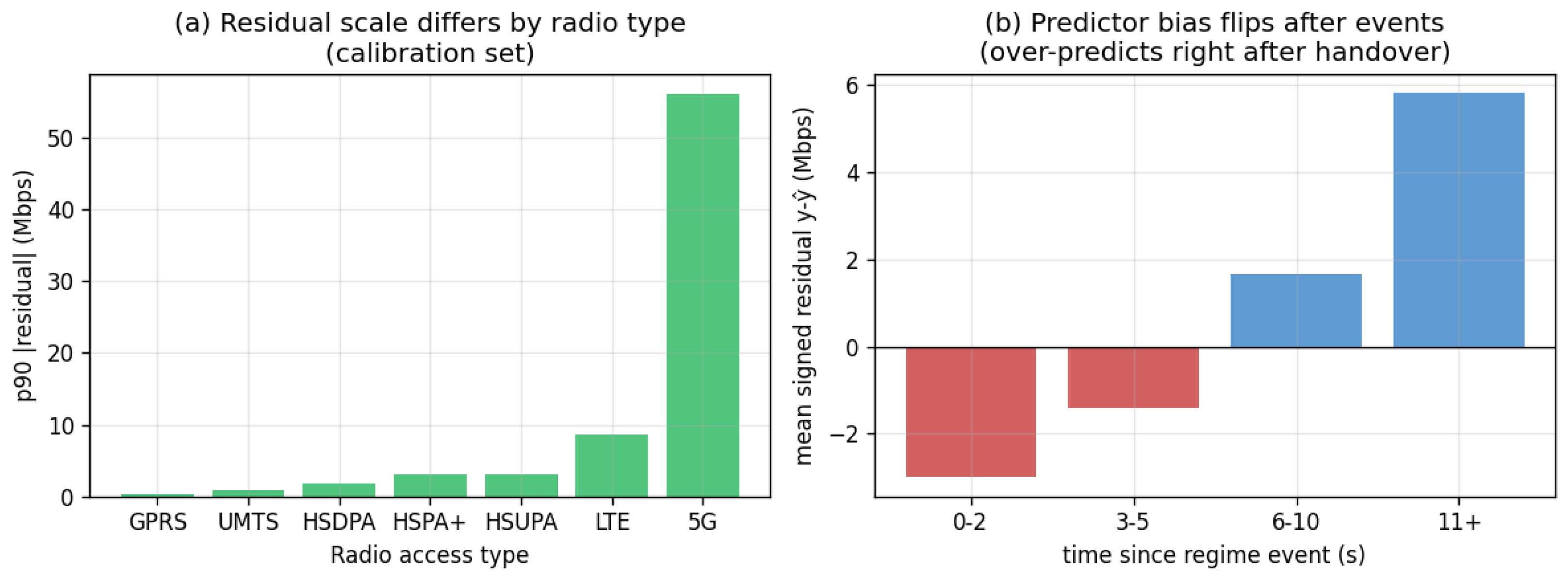
Figure 1 summarizes two significant effects on the calibration set. First, the scale of the base predictor’s residuals differs by an order of magnitude across RATs: the 90th-percentile absolute residual is $\approx 56$, $8.6$ and $3.0$ Mbps for 5G, LTE and HSPA+ respectively (Kruskal–Wallis $H=930.6$, $p\approx 8.5\times {10}^{-203}$). Second, the signed residual $y-\widehat{y}$ flips sign after a regime event: within 5G it is $-4.28$ Mbps in the first 2 s after an event (the model over-predicts, not yet having adjusted to the new regime) versus $+7.80$ Mbps in steady state (Mann–Whitney $p\approx 1.3\times {10}^{-32}$; rank-biserial $0.26$). We note that the naïve premise—that throughput is more volatile right after a handover—was not supported (post-event $|\Delta \mathrm{throughput}|$ was slightly lower, because many handovers occur during idle periods); the tested premise is the residual-distribution shift above.

Figure 1. Base-predictor residuals are regime-dependent (calibration set). (a) 90th-percentile absolute residual by radio access type spans an order of magnitude. (b) Mean signed residual $y-\widehat{y}$ by time since regime event: the predictor over-predicts in the first seconds after a handover and under-predicts in steady state.

4.2. Two-Sided Intervals: Regime Conditioning Rebalances Coverage

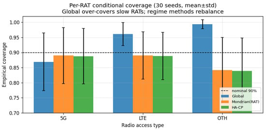
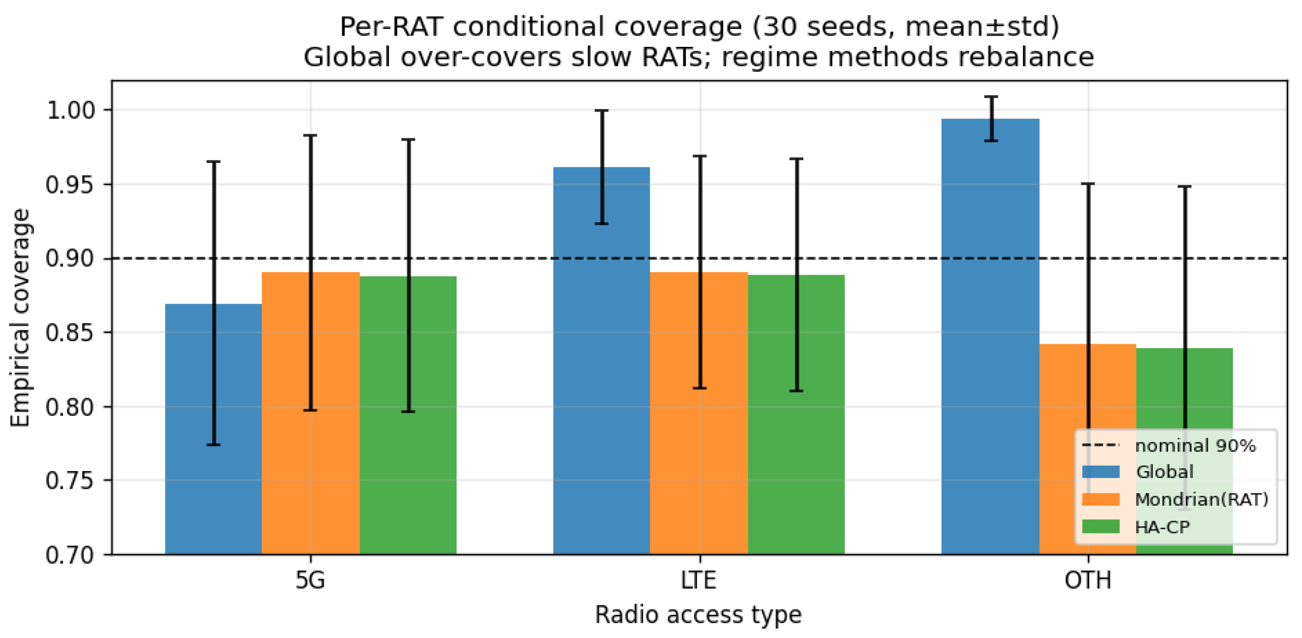
Table 2 and Figure 2 report coverage over 30 seeds at a $90\%$ target. The global interval over-covers slow RATs (LTE $96.2\%$, OTH $99.4\%$): a single global scale forces needlessly wide intervals where the link is stable. Regime conditioning rebalances toward nominal on 5G but then slightly under-covers the slow RATs—the classic Mondrian validity/efficiency trade-off [5], here quantified on real 5G data. Adding the time-since-event split (HA-CP) barely changes the two-sided picture beyond RAT conditioning.

Table 2. Two-sided coverage at nominal $90\%$ (mean over 30 seeds). Global over-covers slow RATs; regime methods rebalance per-RAT coverage.

Method	Marginal	Cov. 5G	Cov. LTE	Cov. OTH	Mean Width (Mbps)
Global	0.897	0.869	0.962	0.994	20.8
Mondrian-RAT	0.885	0.890	0.890	0.841	22.7
HA-CP	0.883	0.888	0.888	0.839	22.7

Figure 2. Per-RAT conditional coverage (30 seeds, mean ± std). The global method over-covers LTE and legacy RATs; regime-conditioned methods move all RATs closer to nominal on 5G at the cost of mild under-coverage on slow RATs.

4.3. Online Adaptive Intervals: HA-CP+ACI Fixes Post-Handover Coverage

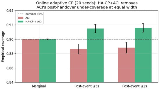
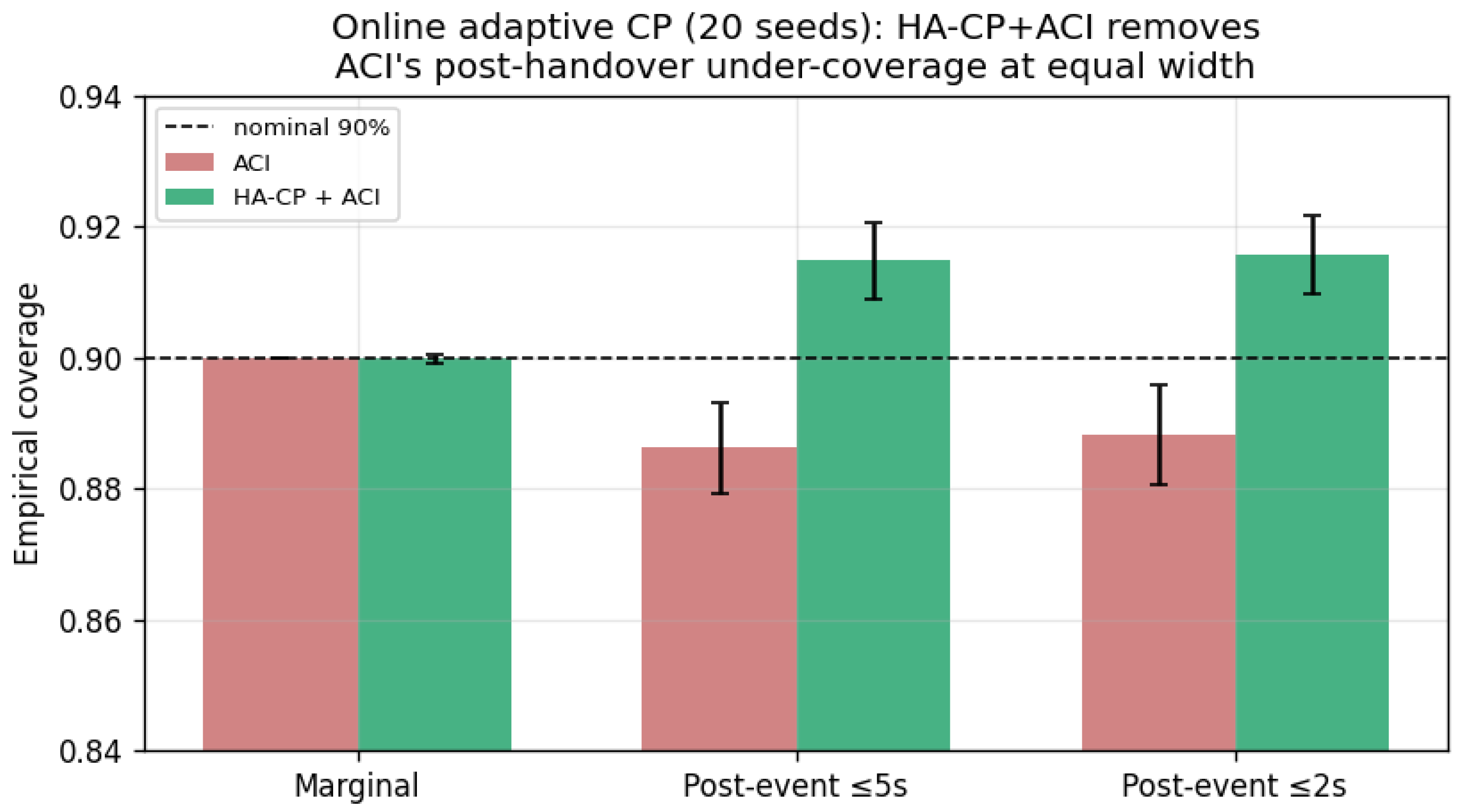
Table 3 and Figure 3 compare ACI and HA-CP+ACI over 20 seeds; we also include DtACI [19], a stronger global adaptive baseline that removes ACI’s single step-size by aggregating a set of ACI experts with different adaptation rates. All three hit (or nearly hit) marginal $90\%$, but the two global online methods—plain ACI and DtACI—systematically under-cover the post-handover window: ACI reaches $88.8\%$ within 2 s and DtACI $87.4\%$, because a global online quantile reacts only after coverage errors, precisely when a handover has just shifted the residuals. DtACI’s expert aggregation improves marginal width efficiency (narrower intervals, $20.3$ Mbps) but does not close the local post-handover gap—if anything it is marginally worse there than plain ACI, since its aggregation is tuned for marginal, not conditional, adaptation. Conditioning the online calibration on regime state (HA-CP+ACI) raises post-event coverage to $91.6\%$/$91.5\%$, eliminating the under-coverage at essentially equal width. The improvement is significant against both baselines (paired Wilcoxon: vs. ACI $+0.027$, $p<{10}^{-5}$; vs. DtACI $+0.041$, $p<{10}^{-5}$; HA-CP+ACI better on $20/20$ seeds in both cases). The lesson is that a stronger global adaptive scheme does not substitute for regime conditioning at the handover: for safety-oriented use, where under-coverage is the dangerous direction, cheap regime conditioning is what fixes the local failure.

Table 3. Online adaptive CP (mean over 20 seeds), nominal $90\%$. Both global adaptive baselines (ACI, DtACI) under-cover the post-handover window; only regime-conditioned HA-CP+ACI removes it, at equal width.

Method	Marginal	Post-Event $\le 2$ s	Post-Event $\le 5$ s	Mean Width (Mbps)
ACI	0.900	0.888	0.886	23.9
DtACI [19]	0.893	0.874	0.876	20.3
HA-CP+ACI	0.900	0.916	0.915	23.4

Figure 3. Online adaptive CP (20 seeds). Both methods meet the marginal target; HA-CP+ACI removes ACI’s post-handover under-coverage at equal width.

4.4. Decision Layer: For a One-Sided Bound, Global Wins

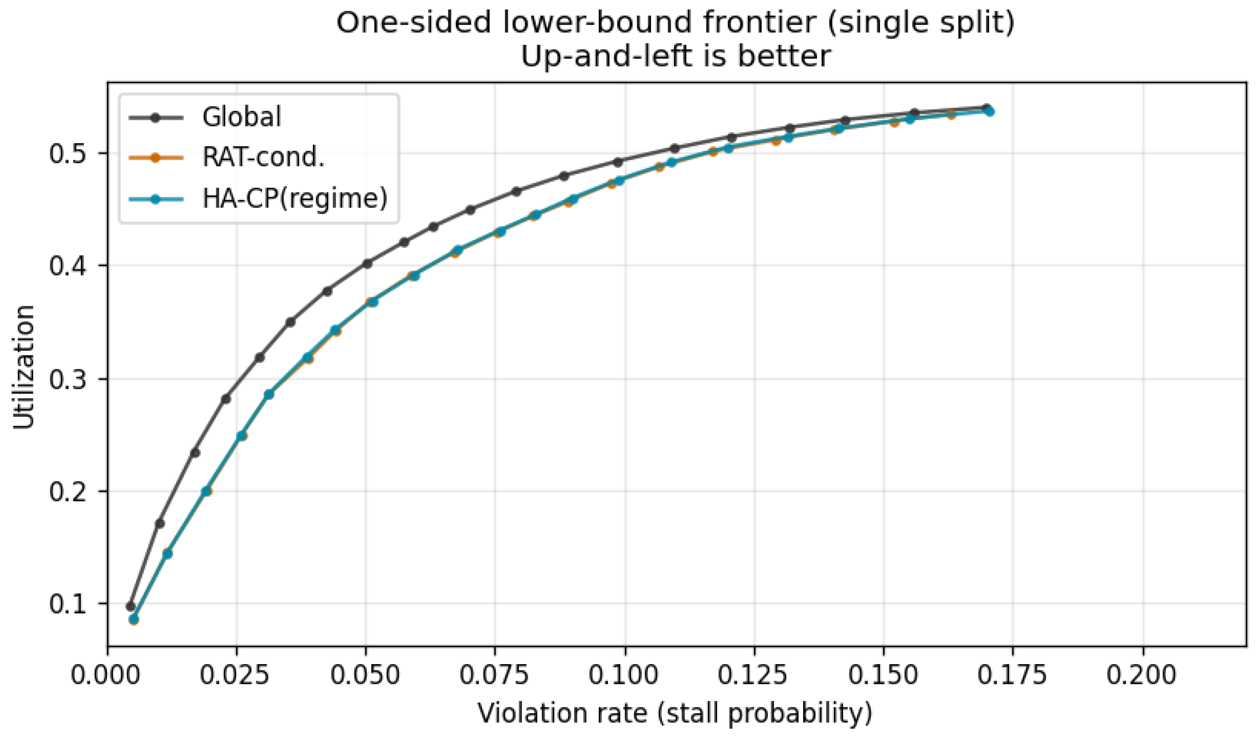
Committing to the point forecast is catastrophic—a $71.5\%$ violation rate—so a calibrated lower bound is essential. Table 4 and Figure 4 and Figure 5 compare one-sided lower bounds on utilization at a matched violation budget (30 seeds). The global bound dominates the regime-conditioned variants at every budget: e.g., $+21\%$ relative utilization at a $2\%$ stall budget. Paired Wilcoxon global-vs-HA-CP gives $p<{10}^{-4}$ at all three budgets (global better on $20/22$, $26/28$ and $25/29$ paired seeds; the paired count is below 30 at the tighter budgets because in some seeds neither method’s frontier reaches so low a violation rate, and those seeds are dropped from the test rather than counted for either side). The mechanism is structural. Rate selection is scored against a marginal violation budget, and the global bound calibrates that marginal quantile directly, whereas the regime variants estimate per-group conditional quantiles—several on small calibration groups (Table 5)—and aggregating these to meet a marginal target sacrifices utilization. We verified that this is an objective-mismatch effect rather than merely inflated estimation variance: the seed-to-seed coefficient of variation of the one-sided quantile is comparable for the global and per-regime estimators ($0.44$ versus a per-state median of $0.40$). The scale heterogeneity that made two-sided Mondrian useful lives in the upper tail (5G bursts), which is irrelevant to a lower bound.

Table 4. One-sided rate selection: utilization at a matched achieved violation budget (mean over 30 seeds; higher is better). The global bound dominates.

One-Sided Method	Util. @ 2%	Util. @ 5%	Util. @ 10%
Global	0.331	0.472	0.569
RAT-conditioned	0.275	0.427	0.549
HA-CP (regime)	0.274	0.427	0.549

Table 4. One-sided rate selection: utilization at a matched achieved violation budget (mean over 30 seeds; higher is better). The global bound dominates.

One-Sided Method	Util. @ 2%	Util. @ 5%	Util. @ 10%
Global	0.331	0.472	0.569
RAT-conditioned	0.275	0.427	0.549
HA-CP (regime)	0.274	0.427	0.549

Table 5. Median calibration-set sizes per grouping over 15 seeds. Several regime states are small, triggering the RAT/global fallback ($\mathrm{MIN}\_\mathrm{GROUP}=50$); this, together with the marginal-budget objective, explains the one-sided disadvantage of partitioning.

Grouping	Calibration Samples (Median)
Global	37,308
RAT: 5G	26,948
RAT: LTE	5312
RAT: OTH	3297
Regime-state (smallest, OTH|3–5)	92
Regime-state (largest, 5G|11+)	25,731

Table 5. Median calibration-set sizes per grouping over 15 seeds. Several regime states are small, triggering the RAT/global fallback ($\mathrm{MIN}\_\mathrm{GROUP}=50$); this, together with the marginal-budget objective, explains the one-sided disadvantage of partitioning.

Grouping	Calibration Samples (Median)
Global	37,308
RAT: 5G	26,948
RAT: LTE	5312
RAT: OTH	3297
Regime-state (smallest, OTH|3–5)	92
Regime-state (largest, 5G|11+)	25,731

Figure 4. One-sided rate selection (30 seeds): utilization at a matched violation budget. The single global lower bound dominates the regime-conditioned variants.

Figure 4. One-sided rate selection (30 seeds): utilization at a matched violation budget. The single global lower bound dominates the regime-conditioned variants.

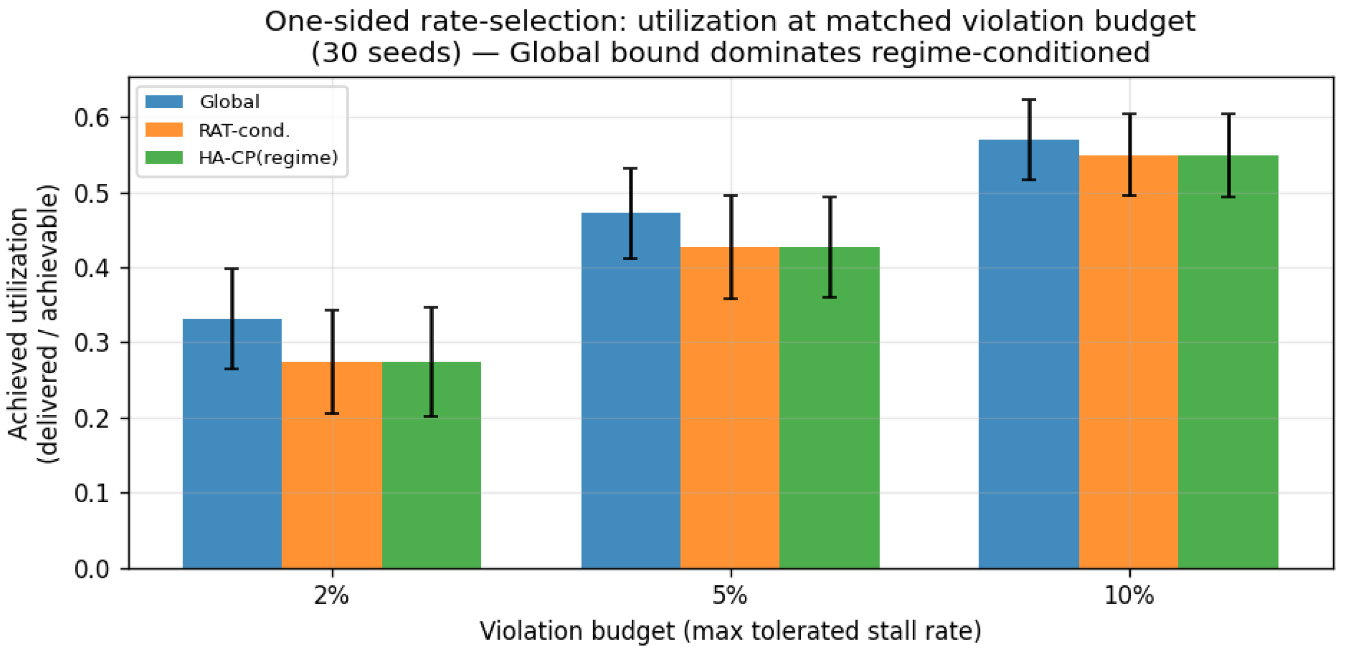
Figure 5. Violation-versus-utilization frontier for one-sided lower bounds (single split). Up-and-left is better; the global bound is on or above the regime-conditioned frontiers throughout.

Figure 5. Violation-versus-utilization frontier for one-sided lower bounds (single split). Up-and-left is better; the global bound is on or above the regime-conditioned frontiers throughout.

4.5. External Baseline: Direct Quantile Regression

The comparisons above are among conformal variants. To place them against a published, non-conformal alternative that also yields intervals and bounds, we add direct quantile regression (QR): gradient-boosting models trained with the pinball loss to predict conditional quantiles of throughput. For fairness the QR models use the same features and hyperparameters as the base predictor and are fit on the train and calibration traces combined—the same total labeled data the conformal method consumes—over the same 30 trace-level splits (Table 6). QR is a natural comparator precisely because it targets quantiles directly, but, unlike conformal calibration, it carries no finite-sample coverage guarantee.

Table 6. External quantile-regression (QR) baseline vs. conformal global (30 seeds). QR over-covers and is wider two-sided, and collapses to zero utilization one-sided under zero-inflation. Lower $|\mathrm{cov}-0.90|$ and higher utilization are better.

Setting	Metric	QR Baseline	Conformal (Global)
Two-sided	Marginal coverage (target $0.90$)	0.948	0.897
	Mean width (Mbps)	23.8	20.8
One-sided	Utilization @ $2\%$ budget	0.000	0.331
	Utilization @ $5\%$ budget	0.000	0.472
	Utilization @ $10\%$ budget	0.000	0.569

For two-sided intervals, the QR band $[{\widehat{q}}_{0.05},{\widehat{q}}_{0.95}]$ over-covers at every seed (marginal $0.948$ vs. the $0.90$ target; $30/30$ seeds above nominal) and is wider than the conformal global interval ($23.8$ vs. $20.8$ Mbps), so on marginal calibration and efficiency conformal is the better choice; QR’s one compensating virtue is more uniform per-RAT coverage, since its conditional quantiles adapt to the input without an explicit grouping. For the one-sided decision bound the gap is decisive: QR’s lower bound is degenerate under the heavy zero-inflation. Because roughly $45\%$ of samples sit at ≤0.001 Mbps, the conditional lower quantiles are essentially zero up to the median, so QR delivers zero utilization at any usable stall budget and only rises above zero at the $0.50$ quantile, where the achieved violation rate has already jumped to ≈0.60 (in all 30 seeds). The conformal global bound, whose offset is calibrated on the marginal residual tail rather than a conditional quantile, sidesteps this collapse and dominates QR on utilization at every budget ($0.33$/$0.47$/$0.57$ vs. $0.00$; paired Wilcoxon $p<{10}^{-7}$, conformal better on all paired seeds). This is the same failure mode that ruled out conformalized quantile regression in Section 3.6, now quantified against a plain-QR baseline. The mechanism is a difference in what is calibrated: quantile regression estimates a conditional quantile of the target, which under this zero-inflation is identically zero for the idle-dominated inputs, so its lower bound is zero until the quantile level is raised so far that the violation rate is unusable (empirically, the first non-zero utilization appears only at the median, where achieved violation $\approx 0.60$). The global conformal bound instead adds a single marginal offset to the point prediction, $L\left(x\right)=\widehat{f}\left(x\right)-Q_{\beta }$; since $\widehat{f}\left(x\right)$ regresses toward the positive conditional mean on active inputs and $Q_{\beta }$ is one fixed scalar, $L\left(x\right)$ remains positive and usable exactly where the conditional lower quantile collapses to zero. Global CP avoids the degeneracy not by being conformal per se, but by calibrating an additive marginal offset rather than a conditional quantile. In short, for risk-sensitive rate selection on zero-inflated throughput, a marginally calibrated conformal offset is not merely a refinement of quantile regression but a prerequisite for a usable lower bound.

4.6. Sensitivity Analysis

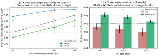
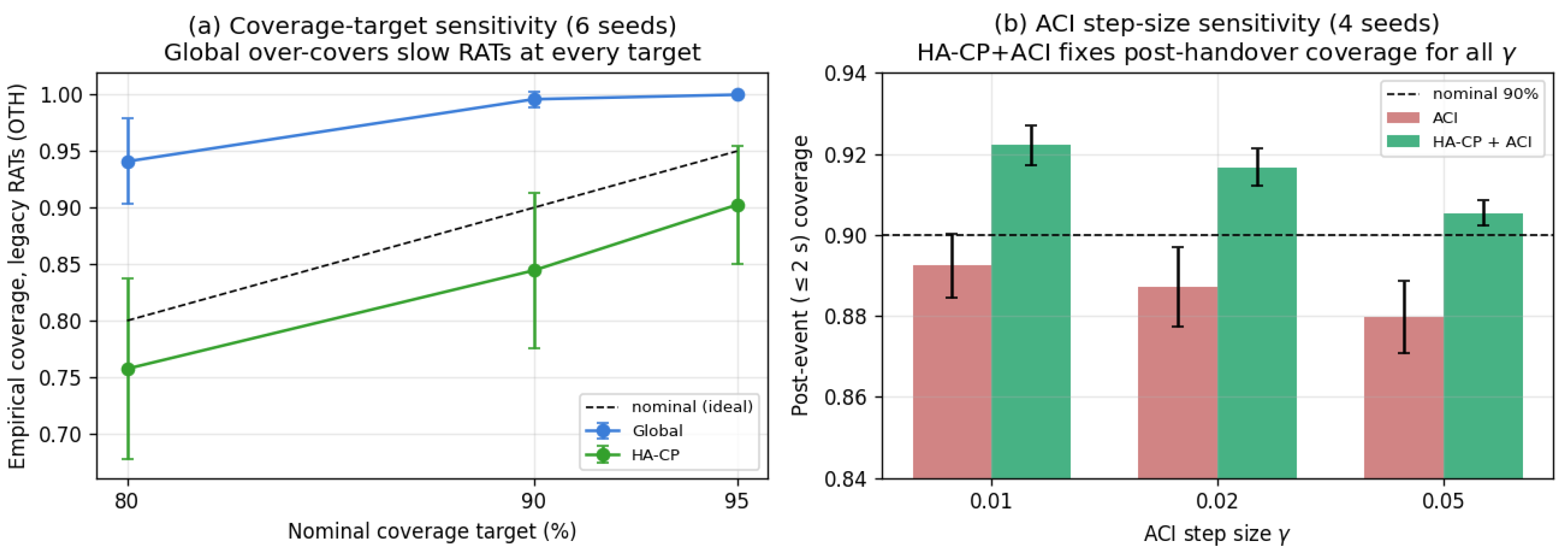
The nominal coverage target ($90\%$) and the ACI step size ($\gamma = 0.02$) were fixed a priori. We verify that the two headline findings do not depend on these choices (Table 7, Figure 6). First, varying the nominal target over $\{80, 90, 95\}\%$ leaves the two-sided pattern intact: the global interval over-covers the legacy (OTH) RATs at every target (empirical coverage $+0.14$, $+0.10$, and $+0.05$ above nominal at $80/90/95\%$), while HA-CP keeps them close to nominal throughout; the over-coverage shrinks at higher targets only because all methods approach $100\%$. Second, varying the ACI step size over $\gamma \in \{0.01,0.02,0.05\}$ leaves the online finding intact: plain ACI under-covers the post-handover window at every $\gamma$ (and progressively more as $\gamma$ grows, $88.0\%$ at $\gamma = 0.05$), whereas HA-CP+ACI restores post-event coverage to near or above nominal, improving on ACI by $+0.026$ to $+0.030$ and winning on all seeds at every $\gamma$. Both main results are therefore robust to the two fixed hyperparameters rather than artifacts of a particular setting. (These sweeps use fewer seeds, 4–6, than the main comparisons because each sweep multiplies the run count by the number of hyperparameter settings; we verified that the reported effects are monotone and consistent across every setting and seed, so additional seeds do not change the qualitative conclusion).

Table 7. Sensitivity analysis. Top: two-sided legacy-RAT (OTH) coverage vs. nominal target (6 seeds). Bottom: post-handover (≤2 s) coverage vs. ACI step size $\gamma$ at nominal $90\%$ (4 seeds). Both findings persist across settings.

Coverage-target sweep: empirical coverage on legacy RATs (OTH)
Nominal target	80%	90%	95%
Global	0.941	0.996	1.000
HA-CP	0.757	0.844	0.903
ACI step-size sweep: post-event (≤2 s) coverage, nominal 90%
$\gamma$	0.01	0.02	0.05
ACI	0.893	0.887	0.880
HA-CP + ACI	0.922	0.917	0.905

Figure 6. Sensitivity of the main findings. (a) Across nominal targets ($80/90/95\%$), the global interval over-covers legacy RATs while HA-CP stays near nominal. (b) Across ACI step sizes $\gamma$, plain ACI under-covers the post-handover window while HA-CP+ACI restores near-nominal coverage. Error bars are ± std across seeds.

The findings are likewise insensitive to the time-since-handover bucket boundaries. Re-running with a finer scheme ($\{0–1, 2–3, 4–7, 8+\}$ s) and a coarse scheme ($\{0–5, 6+\}$ s) in place of the default ($\{0–2, 3–5, 6–10, 11+\}$ s) leaves per-RAT two-sided coverage essentially unchanged (5G $0.900$, LTE $0.868$, OTH $\approx 0.838$ in all three) and preserves the one-sided ordering (global utilization $0.450$ at a $5\%$ budget versus $0.413$–$0.417$ for HA-CP, 8 seeds). This is expected: the two-sided picture is dominated by the RAT axis, and the one-sided bound is regime-invariant in its operative tail, so the sub-bucketing of time-since-handover is second-order.

4.7. Robustness to Zero-Inflation: Active-Traffic Ablation

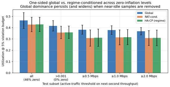
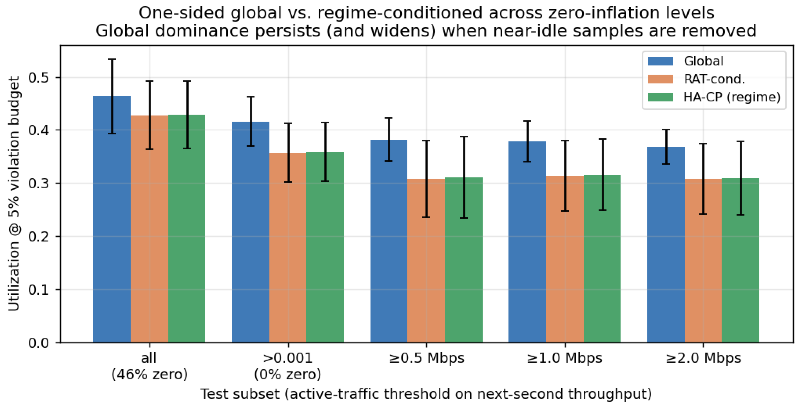
A natural concern is that the one-sided result—global beats regime-conditioned—is an artifact of the dataset’s heavy zero-inflation ($\approx 45\%$ of seconds at ≤0.001 Mbps). We test this directly by removing the near-idle samples: for a throughput threshold $\theta$ we restrict both calibration and test to seconds with $y > \theta$, yielding subsets whose zero-inflation is $0\%$, and re-run the one-sided frontier. Table 8 and Figure 7 report utilization at a $5\%$ stall budget over 15 seeds. The global bound continues to dominate at every threshold; the margin over HA-CP does not shrink but widens, from $+0.035$ on the full data to $+0.057$–$0.071$ on active traffic (paired Wilcoxon $p < {10}^{-3}$, global better on $15/15$ seeds on the de-inflated subsets). The finding is therefore not a consequence of the zeros. The mechanism is that rate selection is scored against a marginal violation budget, which the single global quantile calibrates directly, whereas partitioning the calibration set estimates per-group conditional quantiles that are less efficient for a marginal target—an effect that, if anything, strengthens once the regime-invariant near-idle mass is removed and the RAT-heterogeneous active tail dominates.

Table 8. Active-traffic ablation: one-sided utilization at a $5\%$ violation budget (mean over 15 seeds) on subsets with the near-idle mass removed. Global dominance persists and widens as zero-inflation is eliminated.

Test Subset	Zero-Infl.	Global	RAT-Cond.	HA-CP	Global−HA-CP
All rows	$46.3\%$	0.464	0.427	0.429	$+0.035$
>0.001 Mbps	$0.0\%$	0.416	0.357	0.359	$+0.057$
≥0.5 Mbps	$0.0\%$	0.382	0.308	0.311	$+0.071$
≥1.0 Mbps	$0.0\%$	0.378	0.314	0.316	$+0.063$
≥2.0 Mbps	$0.0\%$	0.368	0.308	0.310	$+0.059$

Figure 7. One-sided utilization at a $5\%$ violation budget as near-idle samples are removed (error bars ± std over 15 seeds). The global lower bound stays above the regime-conditioned variants at every active-traffic threshold, so the finding is not driven by the dataset’s zero-inflation.

4.8. Application-Layer Emulation: Rebuffering and Bitrate

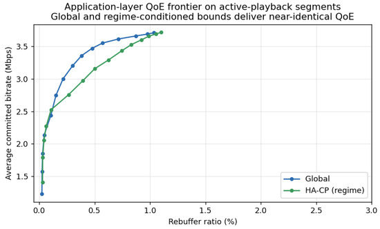
The violation-versus-utilization frontier is the operational metric this paper optimizes, but a reader may ask how the choice of lower bound plays out at the application layer. We therefore emulate a trace-driven adaptive-bitrate (ABR) controller: each second it commits the highest rate on a bitrate ladder ($\{0.3, 0.75, 1.2, 2.0, 3.0, 4.5, 6.0\}$ Mbps) that does not exceed the one-sided bound $L_t$, the link delivers the real trace throughput, and a standard chunk/buffer model accumulates rebuffering time, average committed bitrate, and bitrate-switch rate. This is an emulation, not a full video player. Two findings follow.

First, a QoE simulation over the full traces is not well posed on this dataset: because $\approx$45% of seconds are idle/near-zero throughput, a continuous-playback model spends almost all of its time in apparent rebuffering regardless of the method, and the metric saturates. This is itself a reason we adopt the violation/utilization frontier as the operational objective. We therefore evaluate the emulation on active-playback segments (seconds with $y > 0.5$ Mbps), treating them as continuous playback—an approximation we state plainly.

Second, on those active segments the calibrated bound behaves as intended and the global-versus-regime distinction is immaterial at the application layer. Committing to the raw point forecast rebuffers $\approx$1.3% of the time, whereas the global conformal lower bound (at $\beta = 0.10$) drives rebuffering to $\approx$0%, trading a lower average bitrate for near-elimination of stalls—the safety behaviour a rate-selection bound is meant to provide. Comparing the global and regime-conditioned bounds along the rebuffer-versus-bitrate frontier (Figure 8), they are statistically indistinguishable: at a matched $1\%$ rebuffer budget the global bound delivers $3.57$ Mbps versus $3.52$ Mbps for HA-CP (paired Wilcoxon $p = 0.56$; 10 seeds), with comparable switch rates. Once the raw utilization gap is mapped through a quantised bitrate ladder and a playout buffer, it does not translate into a meaningful QoE difference—which reinforces, from the application side, the practical recommendation to keep the one-sided bound global: it is simpler and no worse.

Figure 8. Trace-driven ABR emulation on active-playback segments (10 seeds). Average committed bitrate versus rebuffer ratio for global and regime-conditioned lower bounds; the two frontiers nearly coincide, so the choice is immaterial at the application layer.

• Why the continuous advantage narrows under discrete ABR.

The apparent tension between the two evaluations—a clear global advantage in the continuous violation–utilization analysis (Section 4.4) that all but vanishes here—is not a contradiction; it is itself an instance of this paper’s central message, and we make it explicit. Utilization is a continuous functional of the lower bound: any change in $L\left(x\right)$, however small, shifts the delivered throughput and is registered one-for-one. The ABR controller instead applies two smoothing operations on top of $L\left(x\right)$ before it can affect experience. First, it quantises the bound onto a finite bitrate ladder, so two bounds that differ by a few percent in continuous utilization often select the same ladder rung and yield identical decisions. Second, the playout buffer integrates throughput over time, so the brief shortfalls that a violation metric counts individually are absorbed by buffered video and never surface as stalls. The ABR objective is therefore far less sensitive to the exact lower bound than the raw frontier is: the global bound’s continuous edge is real, but it falls inside the dead-zone created by ladder quantisation and buffering. This does not reverse the recommendation—global remains no worse under ABR and strictly better on the continuous decision—but it sharpens the paper’s thesis. The magnitude of the benefit from a given uncertainty treatment is set by the downstream decision mechanism: a controller that commits to a near-continuous rate (guaranteed-bitrate admission, uplink-grant sizing) will feel the difference between lower bounds, whereas a coarsely quantised, heavily buffered ABR player largely will not. Practitioners should accordingly match the uncertainty treatment to the granularity and memory of the decision it will drive, not merely to the coverage target.

5. Discussion

We separate three levels of claim: (i) what our experiments demonstrate in the evaluated setting, (ii) how we interpret those results, and (iii) the broader recommendations they suggest, whose generality would require further validation.

(i)

What the experiments demonstrate (evaluated setting).

On the dataset and protocol of Section 3, three effects are statistically supported. First, for two-sided intervals a single global scale over-covers the slow RATs, and RAT conditioning rebalances per-RAT coverage toward nominal (Table 2). Second, for online intervals the two global adaptive methods we tested—ACI and the stronger, aggregation-based DtACI [8,19]—meet their marginal target but under-cover the post-handover window, whereas per-regime conditioning (HA-CP+ACI) restores post-event coverage at essentially equal width (Table 3). Third, for the one-sided bound evaluated on the near-continuous violation–utilization frontier, the global bound attains higher utilization than the regime-conditioned variants at matched stall budgets (Table 4); this ordering persists when the near-idle samples are removed (Section 4.7) but is substantially reduced—to statistical indistinguishability—once the same bound drives a discrete, buffered ABR ladder (Section 4.8). These statements are specific to our single-operator, 2019-era NSA-5G data, client-side KPIs, and single base predictor.

(ii)

How we interpret the results (mechanism; hypotheses).

We offer the following reading as interpretation rather than proven law. Reactive online methods adjust only after coverage errors, so they lag the abrupt residual shift at a handover—which is the mechanism we propose for why per-regime pools, pre-indexed by the observable regime state, close the post-handover gap. On the decision side, rate selection is scored against a marginal violation budget that the global quantile targets directly, whereas partitioning spends calibration data on per-group conditional quantiles, several estimated on small groups (Table 5); we attribute the one-sided ordering to this objective mismatch rather than to inflated quantile variance, which we found comparable across granularities. The compressed phrase “coverage-optimal was not decision-optimal” captures this interpretation in our evaluation: the variant with the best conditional coverage was not the one with the best rate-selection frontier. These directions and magnitudes for mobile 5G were, as far as we are aware, previously unquantified; the underlying trade-offs they echo—Mondrian conditioning exchanging marginal efficiency for conditional validity [5], and one-sided bounds depending on a single tail—are consistent with established theory.

(iii)

What we recommend, and with what caveats.

The practitioner-facing takeaways below are hypotheses supported within our evaluated setting, not validated general design rules, and they are contingent on the downstream decision mechanism. With those qualifications, our results suggest conditioning uncertainty on the radio regime where the objective is two-sided coverage or interval width (e.g., interval-based SLA monitoring); and, for a one-sided rate-selection bound consumed as a near-continuous commitment (e.g., guaranteed-bitrate admission, uplink-grant sizing), that in our data a single global bound was at least as good as regime conditioning and operationally simpler. This last point is explicitly conditional: the global advantage we observed shrank to practical irrelevance once the bound drove a coarsely quantised, buffered ABR player, where the two choices were statistically indistinguishable (Section 4.8). The transferable message we hold most confidently is therefore methodological rather than prescriptive: an uncertainty treatment should be chosen against—and evaluated on—the specific downstream decision it will drive (its operative tail, its granularity, and its memory), not on coverage diagnostics alone. The quantile-regression baseline makes the same methodological point from the other side: a method can target the nominal quantile yet be unusable for the decision (here, collapsing to zero utilization under zero-inflation). Whether the specific orderings we observed transfer to other operators, countries, standalone 5G or 6G, RAN-side KPIs, or other base predictors remains open and would require validation beyond the present evidence.

6. Conclusions

On the real commercial 5G mobility traces we study, the value of conditioning conformal calibration on the mobility-regime state depended on the task. In our evaluation it helped two-sided intervals (rebalancing a severe global over-coverage of slow RATs) and helped online intervals (removing the post-handover under-coverage of the global adaptive methods at no width cost), but it did not help the one-sided lower bound used for rate selection: on the near-continuous violation–utilization frontier a single global bound reached up to $21\%$ higher utilization at a fixed stall budget, an advantage that persisted after removing the zero-inflated samples yet became statistically indistinguishable once the bound drove a discrete, buffered ABR player.

We emphasize the scope of these results. They are demonstrated only for the setting we study: a single commercial operator, one country, and 2019-era non-standalone (NSA) 5G, with client-side (not RAN-side) KPIs and a single base predictor. We frame the practitioner-facing implications as hypotheses supported within this setting rather than validated design rules, and as contingent on the downstream decision mechanism. With those qualifications, our results suggest conditioning uncertainty on the radio regime where the objective is two-sided coverage or interval width, and, for a one-sided rate-selection bound consumed as a near-continuous commitment, that a single global bound was at least as good as regime conditioning and simpler to maintain—a recommendation that weakens or disappears for coarsely quantised, buffered decisions such as ABR. The most transferable takeaway is methodological: an uncertainty treatment should be selected and evaluated against the specific downstream decision it drives, not on coverage alone. We do not claim these findings for standalone (SA) 5G or for 6G. Their extension to those regimes is a hypothesis that requires future validation, not a demonstrated result. The hypothesis is motivated—but not established—by two observations internal to our data: the operative lower tail is set by idle/near-idle periods and by the marginal-versus-conditional calibration trade-off, neither of which is intrinsically NSA-specific; and the one-sided finding survives removal of the zero-inflated samples (Section 4.7). Confirming or refuting it will require SA-5G/6G traces that we could not obtain: to our knowledge no public trace set with per-second client-side KPIs, handover/RAT-change labels, and throughput is currently available for those regimes, and we deliberately did not substitute synthetic data. Generalization across operators, countries, RAN-side KPIs, and alternative base predictors likewise remains open. Releasing our pipeline is intended in part to make such replications straightforward once suitable data appear. The two fixed hyperparameters (the $90\%$ coverage target and the ACI step size $\gamma$), together with the time-since-handover bucket boundaries, were varied in Section 4.6 and left both findings intact.

References

- Narayanan, A.; Ramadan, E.; Mehta, R.; Hu, X.; Liu, Q.; Fezeu, R.A.K.; Dayalan, U.K.; Verma, S.; Ji, P.; Li, T.; et al. Lumos5G: Mapping and Predicting Commercial mmWave 5G Throughput. In Proceedings of the ACM Internet Measurement Conference (IMC), Virtual, 27–29 October 2020; pp. 176–193. [Google Scholar]
- Raca, D.; Leahy, D.; Sreenan, C.J.; Quinlan, J.J. Beyond Throughput, the Next Generation: A 5G Dataset with Channel and Context Metrics. In Proceedings of the 11th ACM Multimedia Systems Conference (MMSys), Istanbul, Turkey, 8–11 June 2020; pp. 303–308. [Google Scholar]
- Raca, D.; Zahran, A.H.; Sreenan, C.J.; Sinha, R.K.; Halepovic, E.; Jana, R.; Gopalakrishnan, V. On Leveraging Machine and Deep Learning for Throughput Prediction in Cellular Networks: Design, Performance, and Challenges. IEEE Commun. Mag. 2020, 58, 11–17. [Google Scholar] [CrossRef] [Scilit]
- Biswas, M.; Chakraborty, A.; Palit, B. A Kalman Filter Based Low Complexity Throughput Prediction Algorithm for 5G Cellular Networks. IEEE Trans. Veh. Technol. 2024, 73, 7089–7101. [Google Scholar] [CrossRef] [Scilit]
- Vovk, V.; Gammerman, A.; Shafer, G. Algorithmic Learning in a Random World; Springer: New York, NY, USA, 2005. [Google Scholar]
- Lei, J.; G’Sell, M.; Rinaldo, A.; Tibshirani, R.J.; Wasserman, L. Distribution-Free Predictive Inference for Regression. J. Am. Stat. Assoc. 2018, 113, 1094–1111. [Google Scholar] [CrossRef] [Scilit]
- Angelopoulos, A.N.; Bates, S. A Gentle Introduction to Conformal Prediction and Distribution-Free Uncertainty Quantification. Found. Trends Mach. Learn. 2023, 16, 494–591. [Google Scholar]
- Gibbs, I.; Candès, E. Adaptive Conformal Inference Under Distribution Shift. In Advances in Neural Information Processing Systems (NeurIPS); Curran Associates Inc.: Red Hook, NY, USA, 2021; Volume 34, pp. 1660–1672. [Google Scholar]
- Sirhan, N.N.; Alrousan, R.; Al-Saqqa, S.; Hamad, F.; Khrisat, Z. Risk-Aware Downlink Throughput Prediction in High-Density 5G Networks. Computation 2026, 14, 105. [Google Scholar] [CrossRef] [Scilit]
- Samba, A.; Busnel, Y.; Blanc, A.; Dooze, P.; Simon, G. Instantaneous Throughput Prediction in Cellular Networks: Which Information Is Needed? In Proceedings of the IFIP/IEEE Symposium on Integrated Network and Service Management (IM), Lisbon, Portugal, 8–12 May 2017; pp. 624–627. [Google Scholar]
- Yue, C.; Jin, R.; Suh, K.; Qin, Y.; Wang, B.; Wei, W. LinkForecast: Cellular Link Bandwidth Prediction in LTE Networks. IEEE Trans. Mob. Comput. 2018, 17, 1582–1594. [Google Scholar] [CrossRef] [Scilit]
- Raca, D.; Zahran, A.H.; Sreenan, C.J.; Sinha, R.K.; Halepovic, E.; Jana, R.; Gopalakrishnan, V.; Bathula, B.; Varvello, M. Empowering Video Players in Cellular: Throughput Prediction from Radio Network Measurements. In Proceedings of the 10th ACM Multimedia Systems Conference (MMSys), Amherst, MA, USA, 18–21 June 2019; pp. 201–212. [Google Scholar]
- Narayanan, A.; Zhang, X.; Zhu, R.; Hassan, A.; Jin, S.; Zhu, X.; Zhang, X.; Rybkin, D.; Yang, Z.; Mao, Z.M.; et al. A Variegated Look at 5G in the Wild: Performance, Power, and QoE Implications. In Proceedings of the ACM SIGCOMM Conference, Virtual, 23–27 August 2021; pp. 610–625. [Google Scholar]
- Minovski, D.; Ögren, N.; Mitra, K.; Åhlund, C. Throughput Prediction Using Machine Learning in LTE and 5G Networks. IEEE Trans. Mob. Comput. 2023, 22, 1825–1840. [Google Scholar]
- Romano, Y.; Patterson, E.; Candès, E.J. Conformalized Quantile Regression. In Advances in Neural Information Processing Systems (NeurIPS); Curran Associates Inc.: Red Hook, NY, USA, 2019; Volume 32, pp. 3538–3548. [Google Scholar]
- Gibbs, I.; Cherian, J.; Candès, E.J. Conformal Prediction with Conditional Guarantees. J. R. Stat. Soc. Ser. B 2025, 87, 1100–1126. [Google Scholar] [CrossRef] [Scilit]
- Xu, C.; Xie, Y. Conformal Prediction Interval for Dynamic Time-Series. In Proceedings of the 38th International Conference on Machine Learning (ICML); PMLR: New York, NY, USA, 2021; Volume 139, pp. 11559–11569. [Google Scholar]
- Zaffran, M.; Féron, O.; Goude, Y.; Josse, J.; Dieuleveut, A. Adaptive Conformal Predictions for Time Series. In Proceedings of the 39th International Conference on Machine Learning (ICML); PMLR: New York, NY, USA, 2022; Volume 162, pp. 25834–25866. [Google Scholar]
- Gibbs, I.; Candès, E.J. Conformal Inference for Online Prediction with Arbitrary Distribution Shifts. J. Mach. Learn. Res. 2024, 25, 1–36. [Google Scholar]
- Tibshirani, R.J.; Foygel Barber, R.; Candès, E.; Ramdas, A. Conformal Prediction Under Covariate Shift. In Advances in Neural Information Processing Systems (NeurIPS); Curran Associates Inc.: Red Hook, NY, USA, 2019; Volume 32, pp. 2530–2540. [Google Scholar]
- Barber, R.F.; Candès, E.J.; Ramdas, A.; Tibshirani, R.J. Conformal Prediction Beyond Exchangeability. Ann. Stat. 2023, 51, 816–845. [Google Scholar] [CrossRef] [Scilit]
- Spiteri, K.; Urgaonkar, R.; Sitaraman, R.K. BOLA: Near-Optimal Bitrate Adaptation for Online Videos. In Proceedings of the IEEE INFOCOM, San Francisco, CA, USA, 10–15 April 2016; pp. 1–9. [Google Scholar]
- Yin, X.; Jindal, A.; Sekar, V.; Sinopoli, B. A Control-Theoretic Approach for Dynamic Adaptive Video Streaming over HTTP. In Proceedings of the ACM SIGCOMM Conference, London, UK, 17–21 August 2015; pp. 325–338. [Google Scholar]
- Sun, Y.; Yin, X.; Jiang, J.; Sekar, V.; Lin, F.; Wang, N.; Liu, T.; Sinopoli, B. CS2P: Improving Video Bitrate Selection and Adaptation with Data-Driven Throughput Prediction. In Proceedings of the ACM SIGCOMM Conference, Florianópolis, Brazil, 22–26 August 2016; pp. 272–285. [Google Scholar]
- Mao, H.; Netravali, R.; Alizadeh, M. Neural Adaptive Video Streaming with Pensieve. In Proceedings of the ACM SIGCOMM Conference, Los Angeles, CA, USA, 21–25 August 2017; pp. 197–210. [Google Scholar]
- Xu, S.; Nikravesh, A.; Mao, Z.M. Leveraging Context-Triggered Measurements to Characterize LTE Handover Performance. In Proceedings of the Passive and Active Measurement Conference (PAM), Puerto Varas, Chile, 27–29 March 2019; pp. 3–17. [Google Scholar]
Disclaimer/Publisher’s Note: The statements, opinions and data contained in all publications are solely those of the individual author(s) and contributor(s) and not of MDPI and/or the editor(s). MDPI and/or the editor(s) disclaim responsibility for any injury to people or property resulting from any ideas, methods, instructions or products referred to in the content. |
© 2026 by the author. Licensee MDPI, Basel, Switzerland. This article is an open access article distributed under the terms and conditions of the Creative Commons Attribution (CC BY) license.