


Abstract
Noise contamination in three-dimensional data remains a persistent challenge in reconstruction and measurement pipelines, with critical implications for dimensional inspection and industrial metrology, as well as for autonomous navigation and cultural heritage documentation. Whenever a point cloud is used to measure rather than merely to visualize, the noise it carries propagates directly into the reported dimension and into its associated uncertainty. This work presents an innovative three-axis taxonomy that unifies the classification and mitigation of noise in 3D point clouds. Our framework systematically categorizes noise sources into (1) statistical models, (2) scene interferences, and (3) reconstruction imperfections, and it is designed so that any newly encountered noise type can be assigned consistently by means of three explicit criteria (origin, modeling tractability and spatio-temporal dependency). Through theoretical analysis along these three axes, we discuss the fundamental limitations, practical challenges, and adaptive strategies of each method and summarize the resulting cross-category applicability in a comparative table. Among the unresolved challenges are real-time processing of dynamic scenes, separation of overlapping noise types, and biases in learning models toward specific sensor geometries. We further argue that, in a measurement context, a denoising operator must be assessed not only by the noise it suppresses but also by the systematic surface displacement—the bias—it introduces, which aggregate distance metrics tend to conceal. This research consolidates fragmented knowledge into actionable guidelines, equipping metrology and inspection practitioners to design robust 3D measurement systems and guiding researchers toward impactful innovations in noise-adaptive sensing.
1. Introduction
Noise in three-dimensional data presents a complex and multifaceted challenge that significantly impacts reconstruction pipelines and downstream tasks such as object interpretation and scene analysis. Point clouds and other 3D representations, including voxels, meshes, and depth maps (e.g., RGB-D, ToF, etc.), are acquired from real-world environments that are inherently imperfect. These data are often corrupted by noise, outliers, occlusions, and clutter, which introduce irregular shadows and incomplete observations. Furthermore, the natural variability of objects, influenced by factors such as viewpoint, illumination, and positioning [1], adds additional complexity to noise characterization and mitigation.
Point clouds are considered the canonical representation of 3D data, as they provide a universal format for translating and unifying all other 3D representations, including raw sensor data, multiple images, depth maps, volumetric data, high-level graph structures, and surface representations such as meshes. This versatility makes point clouds a fundamental abstraction for 3D processing and analysis across various applications. In this work, we focus exclusively on geometric (spatial) noise affecting the positional accuracy of 3D points; noise solely in non-geometric attributes such as color, intensity, or reflectance, while relevant, lies outside the scope of this study.
The impact of this noise is best appreciated through the specific tasks that point clouds now support. In dimensional metrology and industrial inspection, structured-light and fringe-projection scanners are routinely used to verify machined and additively manufactured parts against CAD models, where the reported deviation directly inherits the acquisition noise and its associated uncertainty budget [2,3]; comparative studies of laser scanners against laser trackers with handheld scanning on the same calibrated artifacts show that the choice of instrument alone can shift the achievable dimensional accuracy [4]. In cultural heritage documentation, terrestrial laser scanning and photogrammetry are used to digitize monuments and archaeological sites, where dynamic obstructions from visitors temporarily block parts of the scene and create data gaps that must later be filled [5]. In autonomous driving and mobile robotics, LiDAR point clouds are the primary input to obstacle detection and path planning, and their reliability degrades sharply under fog, rain, and snow, motivating dedicated weather-denoising pipelines trained on datasets such as Weather-KITTI and Weather-NuScenes [6] or on controlled-environment recordings [7]. The same concern extends to underground and infrastructure surveying, where point clouds acquired in geometrically confined roadway environments must still yield usable surfaces, and where recent work has turned to lightweight learned extraction networks precisely because conventional pipelines struggle to eliminate outliers and preserve valid points in complex roadway scenes [8]. In indoor and people-tracking applications built on consumer depth cameras (e.g., Kinect-like ToF and structured-light sensors), the acquired geometry is used to localize and track people or objects in real time, which is why dedicated per-sensor noise models have been developed for this exact use case [9,10].
Adding to these challenges, processing 3D data with complex geometries often incurs high computational costs, limiting real-time applicability—a decisive constraint for in-line inspection, where the measurement must keep pace with the production cycle. Addressing these issues requires robust adaptive frameworks capable of systematically classifying and mitigating diverse noise sources while preserving critical structural information. This work proposes a comprehensive taxonomy and survey aimed at unifying current knowledge and guiding future research in noise-adaptive 3D point cloud denoising methods.
The consequences of noise are particularly tangible when the point cloud is used for measurement rather than visualization, since the acquired coordinates then carry a task-specific uncertainty that must be assessed and declared [11]. In that setting, denoising is not a neutral preprocessing step: filtering too aggressively displaces the surface and biases the reported dimension, so a filter should be judged by the bias it introduces as well as by the noise it removes.
This work classifies noise in 3D data along three main axes—statistical, environmental, and structural—and highlights effective strategies for its mitigation. Our taxonomy organizes fragmented knowledge into a unified framework, enabling the design of robust, adaptive systems for noise handling in diverse 3D sensing applications.
2. Taxonomy of Noise in 3D Data
2.1. Classification Criteria
With the growing adoption of three-dimensional data to tackle challenges once addressed solely through images, the landscape of 3D sensing technologies has expanded at an unprecedented pace. Each sensor, with its own physical principles and limitations, imprints a unique signature on the data it acquires. Structured-light and fringe-projection systems, for instance, recover depth by triangulating a projected pattern, so their error behavior is governed by pattern decoding, projector–camera calibration and the acquisition rate [2,3], whereas laser-based instruments are dominated by range-dependent and incidence-angle-dependent effects. That the resulting differences are substantial, rather than second-order, is borne out by controlled comparisons of instrument classes measuring the same artifacts under laboratory conditions, where a laser scanner and a laser tracker with handheld scanning yield distinguishable dimensional accuracy [4]. Combined with the randomness of environmental conditions and other unpredictable agents, this results in an inherent anti-determinism in 3D acquisition. Yet, within this diversity lies recognizability: noise often carries statistical fingerprints and discernible patterns that, once understood, reveal its origin. Consequently, while some denoising strategies are crafted within the framework of a particular sensor or scenario, others embrace generality, striving to enhance data quality across multiple acquisition technologies. From a metrological standpoint this distinction matters: a sensor-specific model can be tied to a documented calibration and thus contribute an identifiable component to the uncertainty budget of the measurement, whereas a general-purpose denoiser improves the data without, in itself, providing such traceability.
To establish a systematic and reproducible classification framework, we define three fundamental criteria that enable the categorization of any noise type encountered in 3D point cloud processing. These criteria ensure that future noise models can be consistently classified within our taxonomy.
- Origin-based Criterion: Distinguishes noise sources according to their fundamental cause:
- Intrinsic: Noise inherent to the mathematical/statistical nature of the measurement process.
- Extrinsic: Noise caused by external environmental factors during acquisition.
- Systemic: Noise introduced by the acquisition system, processing pipeline, or reconstruction algorithms.
- Modeling Criterion: Evaluates the mathematical tractability and predictability of noise behavior.
- Parametric: Noise that can be described by well-defined probability distributions with estimable parameters.
- Deterministic: Noise with predictable patterns that can be modeled algorithmically.
- Non-parametric: Noise that requires data-driven or empirical modeling approaches.
- Spatio-Temporal Dependency Criterion: Characterizes the correlation structure of noise:
- Independent: Noise affecting individual points without spatial or temporal correlation.
- Structured: Noise that exhibits spatial patterns, temporal evolution, or sensor-specific regularities.
- Global: Noise affecting entire acquisitions or large regions uniformly.
These criteria provide a decision framework where any noise type can be systematically assigned to one of three main categories based on its predominant characteristics. The intersection of these criteria guides the placement within our three-axis taxonomy, summarized in Figure 1.
Figure 1.
Three-axis taxonomy of noise in 3D point clouds. Noise sources are grouped into three categories—statistical models, scene-induced interferences, and acquisition/reconstruction imperfections—each with its dominant character shown underneath. The acquisition/reconstruction category is dominated by deterministic/structured noise, but discrete noise is classified as parametric and independent (see Section 2.4.4). Any newly encountered noise type is assigned by applying the three classification criteria at the bottom, which makes the taxonomy extensible rather than a fixed list.
- Precedence among the criteria.
Because the three criteria are orthogonal, a given noise type will in general receive one label from each of them, and those labels need not point to the same category. We therefore make the arbitration rule explicit, as it governs every assignment made in the remainder of Section 2: the origin criterion determines the category, while the modeling and spatio-temporal criteria characterize the noise within that category. The rationale is that origin is the only criterion tied to the physical mechanism that produces the perturbation, whereas modeling tractability is a property of the description we choose to adopt and may change as better models become available. Two consequences of this rule are worth stating in advance, because they are the source of apparent inconsistencies if the rule is left implicit. First, a noise type may be assigned to the acquisition/reconstruction category on the grounds of its systemic origin while still admitting a perfectly parametric description—this is exactly the case of discrete (quantization) noise, discussed in Section 2.4.4. Second, the modeling label refers to the tractability of the distribution, not to the smoothness or the magnitude of the perturbation: impulsive noise is highly non-smooth yet fully parametric, since a Bernoulli mixture with an estimable corruption rate describes it completely (Section 2.2.4).
- Worked example: classifying a noise type not covered by the taxonomy.
To show that the framework is reproducible rather than a post hoc grouping of the types we happen to review, we apply it to a noise phenomenon that is not among them. Consider mutual interference between two co-located amplitude-modulated continuous-wave (AMCW) time-of-flight cameras observing the same scene with nearby modulation frequencies. The light emitted by the second camera is demodulated by the first as if it were its own returning signal, so the recovered phase—and hence the reported range—acquires a slow beat at the difference frequency, producing depth values that drift coherently over large image regions and over successive frames. Applying the criteria in order: (i) origin is extrinsic, since the perturbing agent is an external emitter present in the scene rather than a limitation of the instrument or of its processing chain, which places the phenomenon in the scene-induced interferences category (Section 2.3); (ii) modeling is deterministic, because once the two modulation frequencies and the relative phase are known the beat is a closed-form function of time rather than a random draw—and it would become non-parametric, not parametric, if those quantities were unknown and had to be estimated empirically from the data; (iii) the spatio-temporal dependency is global, as the beat displaces whole regions of the depth map in the same direction at any given instant, instead of perturbing points independently. The resulting characterization—extrinsic, deterministic, global—immediately carries a practical implication that the taxonomy is meant to expose: a per-point statistical filter is structurally unable to remove this noise, because the corruption is not locally distinguishable from a genuine surface displacement, and mitigation must instead exploit the temporal signature of the beat or coordinate the emitters’ modulation frequencies. The same three-step procedure applies to any newly encountered noise type.
2.2. Statistical Noise Models
This category refers to noise types that arise from the fundamental statistical nature of the measurement process and can be characterized by probability distributions. However, it is important to clarify that these noise models themselves are mathematical constructs designed to approximate the behavior of such noise, rather than phenomena that originate directly from the statistical nature of the process. These noise models generally satisfy the intrinsic origin and parametric modeling criteria and typically exhibit independent spatial behavior. For example, certain noise phenomena, such as those caused by sensor malfunctions, can be effectively approximated by impulsive noise models, even though such models do not represent physically existing noise types.
First, let a 3D point cloud without noise be defined as
2.2.1. Gaussian Noise
Gaussian noise represents the most common statistical noise model in 3D acquisition systems, arising from thermal fluctuations in sensors, quantization errors, and multiple independent error sources following the Central Limit Theorem.
Mathematical Model: Noise follows a multivariate normal distribution , where typically for zero-mean noise. For point clouds, this results in
where is additive, spatially uncorrelated and white (spectrally flat) when is diagonal.
Gaussian noise is said to be isotropic (non-directional) when the variance is equal along all axes, i.e., , which leads to a covariance matrix of the form
This implies rotational invariance; i.e., the noise is distributed equally in all directions, producing a spherical distribution of perturbations around each point. As a type of noise that arises from statistical measurement processes and is characterized by a normal distribution with isotropic covariance, it can be categorized as intrinsic, parametric, and independent.
Otherwise, if the variances differ per axis (), but there are still no inter-axis correlations, the noise is said to be anisotropic (directional), and the covariance matrix becomes diagonal:
This models ellipsoidal noise distributions aligned with the coordinate axes, but still without directional coupling.
More generally, the covariance matrix of a 3D Gaussian noise distribution can be expressed as:
where represent the variances along each axis, and are correlation coefficients that satisfy . This matrix is symmetric () and positive definite, ensuring a valid covariance structure.
The presence of non-zero off-diagonal terms encodes correlations between the axes, which means that the noise distribution may be oriented along directions that do not align with the Cartesian axes. Even if the variances are equal (i.e., the diagonal entries are the same), these correlations break the rotational symmetry of the distribution, making the noise non-isotropic.
A concrete example of a full covariance matrix, used for the non-isotropic Gaussian noise experiments in Section A.1 of the supplementary material in [12], is
Although the variances along each axis are equal (diagonal terms), the non-zero off-diagonal elements introduce cross-axis dependencies. Consequently, the resulting noise distribution is directionally biased and no longer spherically symmetric, hence non-isotropic in nature. In this case, the noise becomes structured.
This general formulation offers a more accurate real-world noise approximation, as practical systems often exhibit correlated noise across dimensions due to shared mechanical or electronic components.
Moreover, empirical evidence supports the Gaussian approximation of Kinect-like depth sensor noise. Park et al. [9] developed a spatial uncertainty model for Kinect sensors, representing measurement error with a full covariance matrix in Cartesian space—effectively modeling noise as multivariate Gaussian. Additionally, Korkalo and Takala [10] proposed a noise measurement model for depth cameras (including structured-light and ToF sensors), where noise in the floor-plane domain is explicitly treated as a 2D Gaussian distribution.
Although most academic articles place particular emphasis on testing models and comparing their performance against synthetic Gaussian noise with zero mean and isotropic standard deviation, this, like other simple parametric distributions, does not faithfully represent complex real-world noise [13,14]. Based on the reviewed literature, a complementary and more demanding validation route—standard in dimensional metrology, but one that we found to be rarely reported in the point cloud denoising studies surveyed here—would be the acquisition of calibrated reference artifacts such as spheres, planes and step gauges, whose true geometry is independently known. Under such a protocol the residual after filtering could be reported as a deviation from a traceable value rather than as a distance to a nominally clean synthetic cloud. We raise this as a direction for future benchmarking rather than as an evaluation carried out in the present work, which is a literature review and not an experimental study; the point is developed further in Section 4.2.
2.2.2. Poisson Noise
Poisson noise typically applies to discrete measurements and is dependent on the signal (amplitude), unlike Gaussian noise, which is additive and signal-independent. It is more suitable for modeling noise in the signal attributes of a point cloud, such as color or intensity, rather than the geometric coordinates that are continuous rather than discrete counts. Emerging from intrinsic signal-dependent processes, this parametric model describes discrete attribute variations through independent Poisson distributions.
Mathematical Model: The noise is based on the Poisson distribution with parameter , where the probability of observing k events is given by the following probability mass function (PMF):
The expected value and variance of the Poisson distribution are:
For a true signal attribute value (e.g., intensity or color) of a point, the noisy observation can be modeled as
where the noise is signal-dependent and non-additive, with variance equal to the mean. Unlike Gaussian noise, it is not spatially uncorrelated in amplitude due to its dependence on local signal intensity.
Poisson noise is ubiquitous in imaging systems [15,16,17,18]. The work in [19] shows that the BM3D (3D Block Matching) filter—originally designed for Gaussian noise removal in 2D images—can be effectively adapted to Poisson noise using variance-stabilizing transformations (VSTs). Although their method operates on pixels, its core idea of grouping similar 3D patches (2D + time/depth) and applying collaborative filtering could inspire analogous approaches for 3D point clouds. In this context, “patches” might correspond to local geometric neighborhoods around each point, with similarity defined via local descriptors (e.g., normals, curvature) or attributes like intensity or color. Indeed, previous methods such as [20] have explored similarities between non-local surface descriptors for denoising 3D unstructured data.
2.2.3. Laplacian Noise
Laplacian noise is additive. It has heavier tails than Gaussian noise and is therefore more robust to outliers. Each point perturbation is an independent draw from a Laplace distribution, so the noise is parametric.
Mathematical Model: The noise vector added to a point follows a multivariate Laplace distribution with zero mean:
where the components are typically independent (spatially uncorrelated) but exhibit stronger deviations than Gaussian noise.
For the univariate case, the Laplace distribution with mean and scale parameter has the following probability density function (PDF):
For multidimensional data, the noise components are often assumed to be independent and identically distributed Laplace variables on each axis.
Laplacian noise is useful when the noise model must account for frequent small errors plus occasional large jumps, unlike Gaussian noise, which heavily penalizes large deviations.
Experimental tests with Laplacian noise are conducted in [21], where it is highlighted that, unlike Gaussian noise, Laplacian noise is sparse but contains larger outliers. Therefore, it is essential to design robust methods that can handle these outliers effectively, allowing for more efficient removal of Laplacian noise without excessively smoothing out the fine details of the point cloud.
Acquired 3D data typically contain small positional errors that can be approximately modeled as zero-mean additive noise—either Gaussian (frequent small errors) or Laplacian (sporadic larger errors). As noted in [21], while complex sensor-specific noise models exist, simpler approximations such as those presented there balance accuracy with computational feasibility. Those extend prior Gaussian-only approaches and establish a more rigorous framework for handling both types of noise.
2.2.4. Impulsive Noise/Outliers
Impulsive noise is non-additive and spatially sparse. Also known as salt-and-pepper noise or outliers, it is characterized by occasional large deviations that do not follow a smooth distribution like Gaussian noise. Its physical causes are heterogeneous—transient sensor dropouts, decoding failures, spurious returns—but what is common to all of them is that the perturbation replaces a measurement instead of adding to it. Applying the criteria of Section 2.1, the phenomenon is intrinsic in origin when it stems from the stochastic failure of the measurement itself, which is why we treat it within the statistical family; it is parametric, because the replacement mechanism is described completely by a Bernoulli mixture whose corruption rate and outlier support are both estimable—the label refers to the tractability of the distribution and not to the smoothness of the realizations; and it is independent in the memoryless case, although, as discussed below, real acquisitions frequently violate this last assumption.
Mathematical Model: Let denote the corruption rate and let be an indicator drawn independently for each point. The observed point is then given by the impulse-replacement model
where is the true coordinate and is a wild (outlier) point drawn from a broad distribution with wide spatial support. The usual choice is a uniform distribution over the axis-aligned bounding box of the clean cloud,
which makes the outliers directionally unbiased; constraining the support to a subset of the axes, or replacing by a heavy-tailed distribution centred on , yields the directional and near-surface variants encountered in practice. Equations (4) and (5) together make the non-additive character of the model explicit: the clean coordinate is discarded rather than perturbed, so a fraction of the points are replaced by outliers randomly distributed in space.
In real-world captures, impulsive noise frequently appears in spatial bursts (e.g., contiguous outlier clusters from transient occlusions or sensor glitches). This suggests extending the Bernoulli model to Markovian frameworks, where outlier probability depends on neighboring point states—akin to Markov–Middleton models in signal processing. Moreover, bursty outliers violate the i.i.d. assumption, necessitating denoising methods that account for local spatial correlations, such as Markov random fields (MRFs) or density-aware clustering [22].
2.2.5. Speckle Noise
Speckle noise is one of the most important forms of multiplicative and spatially correlated noise, so it follows a multiplicative model:
where denotes the clean signal (e.g., geometry or attributes of points), is the noise field, and are the noisy data observed.
Applying the three criteria requires care here, and we state the reasoning explicitly because speckle is the type whose classification is least self-evident. Physically, speckle is the interference pattern produced when coherent illumination is backscattered by a surface that is rough at the scale of the wavelength; the mechanism therefore belongs to the measurement process itself and the origin is intrinsic, which is what places speckle in the statistical family rather than among scene-induced interferences—the scene modulates the effect, but it does not cause it. On the modeling axis, speckle is parametric, consistently with how it is treated in the adjacent fields where it was first characterized: in synthetic aperture radar and in medical ultrasound, fully developed speckle is conventionally described by the Rayleigh distribution of the envelope amplitude and by the Gamma distribution of the multi-look intensity, both of which are closed-form families with estimable parameters. This connects speckle directly to the Rayleigh and Gamma models discussed in Section 2.2.7, of which it is the coherent-imaging instance. Finally, on the spatio-temporal axis speckle is structured and not independent, since the speckle grain has a finite correlation length set by the aperture and the wavelength, so neighboring samples are correlated by construction. The resulting characterization is thus intrinsic, parametric and structured.
We note that the Perlin-based generator used below to simulate speckle is a deterministic algorithm, but this is a property of the surrogate used to inject the noise in controlled experiments, not of the noise being modeled; classifying a phenomenon by its synthesis routine would place any noise type in the deterministic class as soon as a pseudo-random generator for it existed. We therefore classify speckle as parametric and describe the Perlin field purely as a practical, spatially coherent surrogate.
Mathematical Model: To synthesize speckle noise in point clouds, a common strategy is to use Perlin noise, a spatially coherent, gradient-based pseudo-random function originally developed for texture synthesis. Speckle is simulated by applying a Perlin noise field multiplicatively over the surface:
where denotes the m-th octave of the noise function, with frequency and amplitude . Parameters , , and persistence control the level of detail and spatial variation [23]. Essentially, it introduces anisotropic structured perturbations aligned with the surface.
This model yields spatially structured fluctuations that mimic real-world speckle effects and provides a controllable way to introduce non-additive, anisotropic distortions into 3D data.
2.2.6. Uniform Noise
Uniform noise is an additive and bounded noise model commonly used in synthetic experiments to test denoising methods under intrinsic limited but random perturbations. It is characterized by having an equal probability for all values within a fixed interval. This parametric model applies independent uniform perturbations within fixed intervals, representing random uncertainties.
Mathematical Model: Each scalar perturbation is drawn from a uniform distribution over the interval with , whose probability density function is
with mean and variance . This makes the noise non-directional if the interval is symmetric (, hence zero mean) and directional if it is biased (e.g., , which displaces the surface by on average and therefore introduces a systematic bias rather than pure scatter).
When applied to 3D point clouds the three coordinates are perturbed independently, so that the resulting displacement is uniform over the axis-aligned cube :
Some works instead draw the displacement uniformly from a ball of radius r, which removes the axis alignment of Equation (8) at the cost of a slightly less convenient marginal. Either way, uniform noise serves as a useful baseline for controlled noise studies due to its well-defined bounds and simplicity.
The method in [24] shows strong performance against uniform noise (generated by a 3D ball distribution) through its gradient field learning approach. Quantitative evaluation shows good Chamfer Distance and Point-to-Mesh metrics. The key advantages are that the gradient field estimation naturally pulls uniformly distributed points toward the underlying surface without explicit noise modeling, that the continuity-preserving resampling algorithm maintains geometric consistency during denoising and that the method generalizes well to unseen noise types despite being trained only on Gaussian noise. The results confirm the robustness of their physics-inspired approach to uniform noise removal while preserving surface details.
Another physics-inspired approach to uniform noise removal is similar to the approach of [25], which demonstrates effective uniform noise suppression in 2D vector fields through physical constraints (solenoidal projection removing divergent noise components), spectral filtering (preserving large-scale flow structures while attenuating high-frequency noise) and vorticity rectification (enforcing physical consistency). These principles can be directly translated to 3D point cloud denoising by treating point displacements as vector fields and the underlying surface as a physical constraint. The projection operation becomes surface reconstruction (e.g., via MLS or RANSAC), spectral filtering translates to neighborhood-based smoothing that preserves geometric features while reducing random displacements, and the vorticity constraint corresponds to normal/curvature regularization that pulls noisy points toward geometrically consistent positions. This physical-to-geometric analogy provides a robust framework for correcting 3D point displacements while maintaining surface continuity, mirroring how fluid dynamics maintains flow continuity in 2D denoising.
The method proposed in [26], based on norm fitting, is particularly well-suited for inverse problems with this type of noise, as it explicitly accounts for the noise’s bounded support, as the functional constraint focuses on the largest values that the signal takes, ignoring the small fluctuations, and ensuring that the reconstruction tolerates the worst-case perturbation without over-smoothing edges or textures. This framework extends seamlessly to 3D point clouds, where uniform noise arises naturally in spatial coordinates. Here, each point is perturbed independently within a hypercube , and the residual minimization enforces geometric consistency by bounding the maximum deviation across all dimensions. Unlike methods, which are sensitive to outlier perturbations, the approach guarantees uniform data fidelity.
2.2.7. Other Parametric Noise Models of Interest
Beyond the noise models discussed above, the parametric family also includes several distributions that, while not yet tied in the literature to a documented 3D point cloud acquisition or denoising use case, remain of interest because they are the natural extension of well-established models from adjacent signal processing domains (coherent imaging, laser-based sensing…) to the 3D setting, and may become relevant as new sensing modalities are adopted. We group them here rather than granting each its own subsection, precisely because—unlike Gaussian, Poisson, Laplacian, impulsive, speckle, or uniform noise—no cited work currently applies them to 3D point clouds specifically.
Gamma noise is suitable for modeling non-negative, skewed deviations and is relevant in scenarios involving multiplicative effects and photon statistics, typical in laser-based imaging systems, offering a more realistic representation than symmetric additive models. This type of noise originates from intrinsic photon statistics, and parametrically models skewed positive deviations via Gamma distributions:
where k is the shape parameter, is the scale parameter and is the Gamma function. This distribution is also known as Erlang noise in the laser imaging context.
Rayleigh noise arises in magnitude measurements involving coherent signals, such as radar and range imaging, where the underlying complex signal components may be modeled as Gaussian distributions. It is produced by intrinsic magnitude measurements in coherent systems; this parametric noise follows independent Rayleigh distributions:
where is the scale parameter of the noise distribution. This model is often applied to noise in range imaging and radar magnitude data. Rayleigh noise is skewed and strictly positive, capturing the distribution of envelope fluctuations.
Unidirectional noise is additive and axis-aligned, perturbing only one coordinate. It tests the ability of denoising algorithms to handle noise with directional bias and a reduced complexity structure. As it independently adds axis-aligned Gaussian perturbations, this parametric noise simulates intrinsic anisotropic effects. In practice, this is often implemented by adding Gaussian noise only to a single component of each point; for example, the x-component is perturbed as:
where is set as a relative percentage of the bounding region (e.g., the radius of the bounding sphere or the side length of the bounding box) to control the noise intensity. Unlike Gamma and Rayleigh noise, unidirectional noise does have a demonstrated use in the point cloud denoising literature as a synthetic stress test: Luo and Hu use noise levels of 1%, 2%, and 3% of the bounding-region scale to evaluate robustness to directional bias [12].
2.3. Scene-Induced Interferences
This category includes noise that arises from environmental factors and scene characteristics that interfere with the acquisition process. These noise types satisfy the extrinsic origin criterion and typically exhibit deterministic or structured spatial–temporal dependencies.
A qualification applies to this whole category, and it is the same one that we develop quantitatively for the acquisition chain in Section 2.4.1. A scene-induced disturbance does not act on the reconstructed coordinates directly. It acts on a physical quantity measured much earlier in the chain—the irradiance reaching the detector, the visibility of a projected pattern, the shape of the returned pulse—and only reaches the point cloud after that quantity has been transformed by the estimation and reconstruction stages of the instrument. Ambient light from an uncontrolled scene, for instance, does not displace a point: it raises the background level of the captured images, reduces the modulation contrast of the projected fringes, and thereby inflates the variance of the estimated phase, which the triangulation geometry then converts into a depth uncertainty whose magnitude depends on the local geometry of the setup and not only on the strength of the disturbance. The practical consequence is that the same environmental agent produces different coordinate-domain signatures on different instruments, and that the intensity-domain statistics of the disturbance cannot be carried over unchanged to the coordinate domain. Throughout this section we therefore describe the disturbance at its point of entry and, where the literature supports it, its coordinate-domain manifestation separately.
2.3.1. Specular/Reflective Surfaces
Reflective surfaces, such as polished metal, ceramics, or translucent materials, are a significant challenge in 3D scanning due to the way they interact with light, e.g., with laser or natural light. Instead of simply bouncing coherently back to the sensor, these surfaces can scatter or reflect in unexpected and random ways, altering the resulting 3D data. It is categorized as extrinsic (environmental origin), non-parametric (empirical mitigation), and structured (spatial coherence created by complex light-scattering artifacts).
Chen and Shen describe a common issue in this respect [27], which is the presence of long-range outlier noise, i.e., points that appear noticeably far from the true surface. Such outlier-like noise usually results from single reflections, when the laser hits the object at sharp angles, or multiple reflections, when the scanned surface is characteristically shiny. The errors derived from these phenomena can be grouped into two categories: (1) isolated noise points, which are relatively easy to remove using filters that detect distant anomalies, and (2) attached noise clusters, which lie close to the surface and are much harder to remove without altering the true geometry of the object.
But even when the reflectivity involved is not extreme, it is typical that subtle variations in how the light reflects on the surface still cause short-range, high-frequency noise. This distortion usually blurs fine details, but without affecting the overall shape, as also noted in [27].
Another important phenomenon is edge flare—a known effect that occurs near sharp edges or corners (i.e., geometric discontinuities). In these zones, the sensor tends to lose accuracy because of the sharp changes in geometry, scattering light unpredictably, making it impossible in practice to acquire a measurement.
In addition, multi-view stereo (MVS) systems face additional challenges. This is because, according to Berger et al. [28], reflections can change depending on the viewpoint, creating specular highlights that confuse stereo matching procedures and algorithms. This results in structured clusters of false points that may be spatially coherent but do not correspond to the actual surface, worsening the already low reliability of these reconstruction methods for high-precision applications.
The analysis of highly reflective surfaces such as solar panels, polished metals, and ceramics presents unique imaging challenges, as investigated by Zhou et al. [29]. These materials exhibit three characteristic difficulties: intense specular reflections that mask genuine defects and generate false artifacts, extreme sensitivity to environmental conditions where minor lighting or viewpoint changes dramatically alter surface appearance, and complex microstructural properties that introduce high-frequency noise patterns. The combination of these factors renders conventional defect detection approaches ineffective, as they struggle to distinguish between actual surface imperfections and reflection-induced artifacts. Ref. [29] addresses these challenges through an improved Faster R-CNN architecture featuring three principal innovations. First, the framework employs adaptive anchor boxes optimized for micro-defect detection via K-Means clustering. Second, it implements a hierarchical feature fusion approach that combines multi-scale visual information to differentiate true defects from reflection noise. Third, the system incorporates illumination-invariant training protocols to maintain stability in varying lighting conditions. While originally developed for defect identification, this methodology’s robust handling of reflective surface artifacts suggests promising applications in 3D point cloud denoising, particularly for scenarios involving specular materials where traditional noise removal techniques often fail.
Finally, translucent materials introduce yet another layer of difficulty. In this sense, light does not just reflect off them, but it penetrates and scatters within. Ref. [27] highlights that this internal scattering, combined with external reflections, creates both long-range outliers and dense patches of short-range noise, seriously compromising the quality of CAD or metrology scan scenarios.
Surfaces of this kind—specular, transparent or translucent—are collectively termed non-collaborative, and they are the standard failure case of optical acquisition. The recent turn towards learning-based reconstruction does not by itself resolve the problem: such methods can produce visually plausible geometry where classical pipelines fail outright, but their dimensional fidelity has to be quantified separately and does not follow from perceptual quality [30].
2.3.2. Dynamic Obstructions
Dynamic obstructions refer to transient, moving objects—such as pedestrians or vehicles [5]—that interrupt 3D scanning and appear as spurious clusters of outliers. Unlike static noise, these obstructions manifest briefly and unpredictably, often creating temporary point clusters or ghost points that drift in and out of the scanned data. These artifacts require multi-frame, time-aware filtering strategies, since single-frame denoising is usually insufficient. As noted in [6], these artifacts manifest themselves as structured but transient anomalies that confuse downstream tasks such as semantic segmentation and object detection, which makes it vital to suppress them. In this sense, it is classified under extrinsic sources with non-parametric modeling and structured dependencies, as transient objects create spatiotemporal outlier clusters.
Although they form clusters similar to surface outliers, dynamic obstructions differ because they disappear suddenly, introducing temporal discontinuities in the noise pattern. This erratic behavior sets them apart from other ones like persistent geometric noise or seasonal environmental artifacts. Moreover, each point cloud frame is usually irregularly sampled, and different frames may exhibit varying sampling patterns with possibly different numbers of points, which means there is no explicit temporal correspondence between points over time, which complicates the task [31].
Dynamic obstructions are particularly problematic because they do not maintain consistency over time. Their presence in one frame and absence in the next can create discontinuities that are difficult to distinguish from genuine scene features or legitimate structures. This requires the development of specialized techniques to effectively identify and mitigate their impact.
Additionally, motion blur artifacts—caused by relative movement between the sensor and objects during acquisition—can manifest as elongated point clusters or smeared surfaces. These effects share similarities with dynamic obstructions, but arise from temporal integration rather than physical occlusions, requiring motion-aware reconstruction or deblurring techniques.
Furthermore, Chen et al. highlight an additional issue with Terrestrial Laser Scanning (TLS) point clouds [5]. In uncontrolled scenes, the scanned data often suffer from irregular data gaps due to moving objects like pedestrians or cars, leading to a loss of integrity and quality, and since dynamic occlusions are transient, they create gaps that must be identified and filled in order to achieve accurate reconstructions. This makes it essential to develop effective techniques to handle such cases.
2.3.3. Light Interference
Light scattering can also cause the appearance of long-range noise in scanned objects [27]. A well-known effect is edge flare, which refers to aggravated errors at sharp edges or corners (geometric discontinuities) caused by light scattering. This phenomenon leads to a loss of measurement accuracy in these regions due to the sensor’s reduced ability to capture precise data, all due to the lighting or reflective nature of the surface or artifact in the scene [32].
So, exhibiting extrinsic, non-parametric, and structured traits, scattered light usually induces edge flare artifacts at geometric discontinuities.
2.3.4. Temperature Variations
Temperature variations are an extrinsic and deterministic noise source that globally affects 3D point cloud data, particularly in sensor-based acquisition systems. These thermal shifts cause systemic calibration drifts in LiDAR or structured-light sensors, leading to inaccuracies in depth measurements and introducing distortions in the captured 3D surface geometry. They act on the instrument and on the workpiece alike, since thermal expansion of the measured part displaces the very surface being sampled; this is why dimensional measurements are conventionally referred to a reference temperature of 20 °C, and it is also why departures from controlled shop-floor conditions cannot be treated as ordinary random noise.
Unlike random noise, temperature-induced errors follow predictable patterns but require specialized denoising approaches to correct without compromising fine structural details. As demonstrated by Ding et al. [33], temperature fluctuations produce distinct noise patterns in 3D scans, where the authors use statistical thresholds to automatically detect and filter these thermal artifacts, enabling accurate surface reconstruction while maintaining critical micro-texture details.
The method in [33] tackles temperature-related 3D noise using a two-step approach. First, it applies a modified Gaussian filter that ignores extreme values (common in temperature errors) by setting the kernel’s center weight to zero. Second, it detects outliers, points with values three times higher than average, and replaces them with neighborhood averages. It also uses coefficient of variation (CV) analysis to spot smaller local errors without affecting real surface details. Tests prove this method outperforms traditional filters on real surfaces, and it preserves original texture better while effectively removing temperature errors. It handles both gradual temperature changes (with the Gaussian filter) and sudden sensor errors (with CV detection).
2.3.5. Vibrations or Mechanical Instability
Demonstrating extrinsic, deterministic, and structured behavior, mechanical resonances produce spatially correlated distortions in the point cloud. This noise source is prevalent in mobile mapping systems, such as UAVs or handheld scanners, where the platform’s engine or movement introduces high-frequency oscillations to the sensor’s pose during acquisition.
Unlike random noise, these vibrations do not affect points independently. Instead, they manifest as wave-like patterns or “ripples” on otherwise planar surfaces, strictly following the scanning trajectory. Since the error depends on the platform’s oscillation frequency and the specific timestamp of the measurement, the resulting distortion is highly structured and predictable, often requiring trajectory smoothing or inertial data fusion for correction rather than simple local averaging.
2.3.6. Adverse Weather
Qualified as extrinsic, non-parametric, and structured noise, adverse weather conditions, such as atmospheric particles, rain, fog, and snow, create localized interference patterns and introduce noise into scanned point clouds, significantly degrading their quality and reliability for downstream perception tasks in autonomous driving and robotics. Environmental particles scatter, absorb, or anomalously reflect laser pulses (for example), generating false returns and occluding true surface geometries. Unlike intrinsic sensor noise (e.g., Gaussian noise), adverse weather effects exhibit spatial and temporal correlations, making them challenging to filter using traditional statistical or geometric heuristics.
As noted in [6], the noise characteristics vary significantly between different weather conditions. Weather-induced noise points are predominantly concentrated near the LiDAR sensor, and snow produces more dispersed and irregular patterns than rain or fog; across conditions, the corruptions combine substantial spurious returns with missing points. In [7], intensity-dependent spatial correlations are leveraged to distinguish fog particles from valid surfaces, while TripleMixer employs a hybrid geometric–spectral approach to decouple weather-induced artifacts from true geometries in both the spatial and frequency domains.
The development of large-scale datasets (e.g., Weather-KITTI, Weather-NuScenes, etc.) [6] with point-level weather annotations has further enabled data-driven solutions, overcoming the limitations of synthetic simulations and small-scale real-world collections.
2.4. Acquisition/Reconstruction Imperfections
This category encompasses noise introduced by the acquisition system itself, reconstruction algorithms, and processing pipelines. These noise types satisfy the systemic origin criterion and often exhibit structured or global spatial dependencies.
2.4.1. Structured/Sensor-Specific Noise
Structured noise commonly originates from real LiDAR-type sensor acquisitions, which is why it is also referred to as sensor-specific noise. It is characterized by depth-dependent, angular, or sparse perturbations. Empirical studies such as that of Ji et al. [34] have demonstrated that the measurement noise in LiDAR sensors increases with distance due to a lower signal return strength, resulting in range-dependent noise patterns. It also suffers from angular noise caused by the discrete scanning mechanism. The study by Pomerleau et al. [35] further shows that different commercial sensors exhibit distinct error patterns depending on the model, distance, incidence angle or the type of material being scanned. These errors are not random, but systematic and depend on the sensor, the surface, and lighting conditions.
Beyond intrinsic sensor limitations, environmental and operational factors can exacerbate structured noise. Low illumination, high ambient or sensor temperatures, dust or airborne particles, and transmission interference may degrade the measurements. Acquisition conditions can excite intrinsic speckle or Poisson-like fluctuations and shape them into observable patterns; the systemic category captures the resulting structured acquisition artifact, not the intrinsic noise type itself. Impulsive failures and semi-deterministic spatially correlated patterns can also arise under these conditions, and they are treated here as structured acquisition artifacts.
In [36], they attempt to generalize Gaussian noise and address structured noise at high levels. Specifically, they train their model with simulated noise on a LiDAR dataset by scanning ShapeNet objects with a Velodyne HDL-64E scanner using Blensor software [37]. They consider two sources of noise: a laser distance bias modeled as a Gaussian distribution and Gaussian noise added per laser beam (both distributions are set with zero mean and a standard deviation proportional to the region of interest). Similarly, in [24], Blensor is also used to simulate LiDAR noise: point clouds are sampled from meshes at several resolutions, normalized into a unit sphere, and acquired with a virtual Velodyne HDL-64E2 scanner at a fixed noise level.
Similarly, stripe noise in 2D images is widely recognized as structured noise, as noted by [38], while ref. [39] extends this understanding to 3D imaging, categorizing it as sensor-specific noise arising from hardware imperfections or interference. This noise manifests itself as depth/angle-dependent stripe patterns with varying widths and intensities, systematically degrading image quality due to deterministic sensor limitations. To address this, ref. [39] proposes a dual-resolution 3D U-Net model (USRL) that directly learns and removes multiscale 3D stripes through hierarchical feature extraction, coupled with nonlinear dynamic range normalization to adapt to diverse stripe intensities. Their approach outperforms conventional methods (e.g., DnCNN [40]) by preserving structural details while eliminating artifacts, as demonstrated in LSFM neural data, and offers extensibility to other modalities like infrared or medical imaging despite current limitations in processing wide stripes or low-light conditions.
- From detector noise to coordinate noise: the propagation chain.
The discussion above, and indeed most of the denoising literature, describes sensor-specific noise by its appearance in the final point cloud. That description is convenient but incomplete, and for phase-based optical instruments it can be actively misleading. The perturbation does not originate in the coordinate domain at all: it originates in the detector, and what reaches the point cloud is the image of that perturbation under a sequence of transformations performed by the instrument. Making this chain explicit is central to the argument of this survey, because it is what justifies treating point cloud noise as the terminal result of a measurement chain rather than as an additive corruption of an otherwise clean geometry.
Fringe projection profilometry (FPP) is the clearest case, and also the best characterized: a complete precision model chaining the successive stages has been established for it, decomposing the problem into stage models for the camera intensity, the fringe intensity, the phase and the 3D geometry, together with the transfer models that connect them [41]; a subsequent unification shows that the precision models of the vertical-, horizontal- and optimal-angle-fringe reconstructions reduce to a common formulation [42]. We adopt this chain as a conceptual/analytical model for FPP, not as a new experimental result of the present survey. The chain proceeds as follows:
Each arrow is a distinct transformation rather than an identity, and two of them are worth writing out. For an N-step phase-shifting scheme in which the captured intensity at a pixel is , with A the background and B the fringe modulation, propagating the intensity variance through the standard arctangent phase estimator gives
so that the phase uncertainty is governed not by the absolute detector noise but by the ratio between that noise and the local fringe modulation. The triangulation stage then maps the phase uncertainty onto the reconstructed coordinate. To first order, and writing for the sensitivity of the recovered depth to the phase at the point considered, this is
where ℓ is the standoff distance, d the projector–camera baseline and the effective fringe period on the object. Composing Equations (10) and (11) yields , which already exhibits the properties that a purely coordinate-domain noise model cannot represent.
Three consequences follow, and they bear directly on how denoising methods should be designed and assessed. First, detector noise is not simply additive on the final coordinates. It is additive on the intensity; the coordinate-domain effect is the result of a non-linear estimator followed by a geometry-dependent scaling, and the composed operator is neither additive nor, in general, shift-invariant over the measurement volume. Second, the resulting coordinate noise is signal-dependent and spatially non-stationary. Through the factor in Equation (10), the local surface reflectance, the local albedo and the local contrast of the projected pattern all modulate the noise magnitude; through the factor in Equation (11), so does the position of the point within the measurement volume. A dark, steeply inclined, or distant region is therefore noisier than a bright frontal one by an amount that is predictable from the instrument model, which is precisely the kind of structure that an i.i.d. Gaussian assumption discards. Third, the coordinate-domain distribution need not be Gaussian even when the detector noise is. Camera noise is itself a mixture of a signal-dependent photon (shot) component and a signal-independent read component, so is a function of the local intensity rather than a constant; passing such a mixture through the arctangent estimator produces a phase error that is only asymptotically normal, and the approximation degrades exactly in the low-modulation regions where the noise matters most.
The practical implication for the present survey is twofold. On the modeling side, the near-universal practice of validating denoisers against zero-mean isotropic Gaussian noise added directly to the coordinates evaluates them on a corruption that no phase-based instrument actually produces; the discrepancy is not a matter of the noise level chosen but of its structure. On the mitigation side, the chain also indicates where the leverage lies: because depends on quantities that are known or measurable at acquisition time—the modulation B, the number of steps N, the baseline-to-standoff ratio—a per-point uncertainty can in principle be propagated forward and handed to the denoiser as a prior, instead of being discarded and then partially re-estimated from the geometry. This is the concrete form taken, for the FPP case, by the uncertainty-propagating denoisers we advocate in Section 4.2, and it is the sense in which point cloud noise is best understood as a chain-of-measurement result rather than as terminal coordinate noise.
Two additional sensor-specific noise types are shot noise and quantization noise. Shot noise, fundamental to photon-counting sensors like LiDAR, follows Poisson statistics and becomes dominant under low-light conditions, creating signal-dependent variance that scales with measurement intensity. Quantization noise represents systematic errors introduced by analog-to-digital conversion, particularly impactful in time-of-flight (ToF) sensors where depth discretization creates stair-step artifacts at quantization boundaries. Both noise types exemplify how sensor physics imposes structured error patterns that require specialized modeling for effective mitigation.
2.4.2. Data Gaps
Resulting from systematized occlusions or acquisition failures, these deterministic artifacts produce missing-structured regions that often follow the scanning geometry or motion pattern. Data gaps are therefore systemic, deterministic, and structured/global. Such gaps can severely hinder subsequent processing steps by breaking surface continuity and removing critical geometric cues.
The method proposed in [43] targets point cloud denoising with sharp-feature preservation. It defines discrete second-order operators on point clouds to regularize the normal field, detects geometric features via a bi-tensor voting scheme, and repositions points with a RANSAC-based multi-normal strategy. Validated on synthetic Gaussian noise, impulsive outliers, and unorganized point sets, including Kinect scans, the method processes raw point clouds directly without relying on global topology.
In addition, TP-NoDe [44] handles data gaps using its noise-denoising upsampling approach. The method injects controlled noise into sparse regions and applies denoising to reconstruct the underlying surface geometry. This process naturally fills missing areas while preserving sharp features and surface continuity. The progressive refinement strategy enables effective reconstruction of incomplete scans without requiring explicit gap-filling algorithms or complex preprocessing steps.
2.4.3. Scan Stitching Errors
Scan stitching errors manifest as misalignments and geometric inconsistencies when fusing data from multiple depth sensors, such as in multi-camera Poisson reconstruction setups. These errors are systemic, deterministic, and structured/global, arising from calibration inaccuracies, temporal synchronization issues, and sensor-specific noise patterns. Because registration error accumulates along the chain of pairwise alignments, it frequently dominates the overall length-measurement error of a multi-view scan: the point-level repeatability of the sensor may lie well below the residual misalignment between views, so the achievable dimensional accuracy over the whole part is set by the registration stage rather than by the individual acquisitions. This is precisely why the acceptance testing of optical 3D coordinate measuring systems evaluates length measurement error on calibrated artifacts spanning the whole measuring volume, rather than local point-cloud quality alone [45].
These errors often create “balloon-like” artifacts in empty regions where depth measurements conflict, or strongly directional and artificial patterns and clusters of outliers, as shown in [46].
Although traditional approaches often address these problems through post hoc point cloud denoising, recent methods—such as [47]—focus on improving calibration and 3D data recovery during multi-view reconstruction itself. By refining alignment parameters through Kalman filtering and leveraging auxiliary data (e.g., reflectance images or geometric constraints), these techniques reduce stitching errors at the source rather than correcting them after the fact, not only minimizing artifacts but also preserving structural integrity, particularly in large-scale scans where error accumulation is a major concern.
Zhu et al. introduce an innovative stitching methodology [48] for 3D point clouds using PDE-based analytical solutions. Their approach fundamentally addresses the stitching problem by enforcing geometric continuity through explicit PDE solutions that mathematically guarantee smooth transitions between stitched patches. Unlike conventional stitching techniques that rely on iterative alignment, this method formulates the stitching process as a boundary-value problem where the PDE solutions automatically maintain both positional and tangential continuity at stitch boundaries, although the implementation focuses on basic stitching scenarios (single-patch reconstructions).
2.4.4. Discrete Noise
Discrete noise refers to perturbations in which point displacements occur only at a finite set of fixed offsets rather than continuously across a range. This type of noise can model sensor errors that produce quantized, atypical, or degenerate measurements, often due to digitization or mechanical constraints.
Its placement in this category rather than among the statistical models of Section 2.2 follows the precedence rule of Section 2.1. On the modeling axis discrete noise is parametric, and on the spatio-temporal axis it is independent in its basic form; what decides the category is the origin criterion, since the finite set of admissible displacements is an imprint of the instrument—the finite step of an analog-to-digital converter, of an encoder, or of a mechanical indexing stage—rather than a property of the measurand. Discrete noise is thus classified as systemic, parametric and independent.
Formally, the noise distribution is defined as a discrete probability mass function (PMF) on a finite set of displacements :
where s is a scale parameter that controls the magnitude of the displacements. Any displacement not explicitly listed among the has zero probability of occurring, and the perturbed point is obtained as with drawn from Equation (12).
For example, in [12], the simplified discrete noise model displaces points by along each of the three coordinate axes with probability 0.1 each, and leaves them unchanged with probability 0.4:
where the six non-zero displacements and the null displacement satisfy the normalization . The model captures the non-continuous, quantized perturbations that arise whenever the reported coordinate is constrained to a lattice, and it is a convenient stress test precisely because its support is a finite set of offsets rather than a continuous neighborhood.
3. Noise Mitigation Techniques
This section provides a comprehensive review of published denoising and filtering techniques organized by their applicability to the noise categories established in our taxonomy. We analyze computational complexity, parameter sensitivity, and cross-noise category effectiveness for each approach.
3.1. Gradient-Guided Point Set Resampling
Ref. [24] proposes a probabilistic denoising framework that reformulates point cloud restoration as gradient ascent on the log-density of a noise-convolved distribution . Their method demonstrates effective performance across multiple noise types, including isotropic Gaussian noise, Laplace noise, discrete noise, anisotropic Gaussian noise, uni-directional Gaussian noise, uniform noise, simulated LiDAR noise, and real-world noise. It particularly excels against structured parametric noise (e.g., anisotropic/discrete) and scene-induced interferences (e.g., LiDAR artifacts).
Statistical Noise Mitigation: For parametric noise models—such as isotropic Gaussian, Laplace, or uniform noise—the method’s mode-seeking gradient ascent is theoretically grounded in the observation that the clean surface corresponds to the mode of . By iteratively moving points along the gradient , it avoids shrinkage artifacts common in displacement-based methods (e.g., PCN [49]). This is especially effective for Laplace noise with heavy tails, where the continuity of the gradient field (enforced by cosine annealing) prevents over-smoothing while preserving outliers near the surface.
Structured and Scene-Induced Noise: The global gradient field estimation of the method proves critical for anisotropic Gaussian noise and discrete directional noise (both classified as structured). Unlike local operators (e.g., bilateral filtering), the global field aggregates features from all neighbors within the radius r, weighted by cosine annealing to ensure continuity. This allows the model to handle directionally varying corruption—such as anisotropic covariance or discrete spikes along axes—without assuming noise symmetry. For real-world LiDAR noise (a scene-induced interference), the adaptability of the gradient field to local geometry mitigates scanline artifacts and irregular shadows.
Systemic and Non-Parametric Noise: While the method is trained only on Gaussian noise, its regularization-flexible resampling generalizes to non-parametric noise (e.g., Paris-rue-Madame real-world data). By alternating gradient ascent with Graph Laplacian Regularization (GLR) or Reweighted GLR (RGLR), it adapts to unstructured corruption during inference. RGLR’s dynamic edge weights are pivotal for acquisition imperfections, such as inhomogeneous density or sensor-specific artifacts, as they iteratively refine the underlying graph to preserve sharp features.
Computational Trade-offs: Iterative resampling (50+ steps) incurs higher costs for global noise (e.g., uniform spatial corruption) compared to feedforward networks. However, the authors argue that this is justified for structured noise where local methods fail. The continuity constraint improves robustness on anisotropic noise by preventing abrupt gradient changes near the surface boundaries.
Most of the time, this framework excels where noise exhibits directional structure (anisotropic/discrete) due to global gradient estimation; parametric heavy tails (Laplace), through robustness to outliers; and scene/systemic patterns (LiDAR/reconstruction artifacts), through adaptive regularization. Its limitations comprise computational cost and initialization sensitivity.
3.2. Graph-Convolutional Point Denoising Network
Structured Systemic Noise: GPOD [50] presents a method with distinct architectural advantages that make it particularly effective against different types of noise. Its performance is most notable when dealing with structured systemic noise, such as the spatially correlated artifacts found in LiDAR acquisitions. The network excels in this category due to its dynamic graph construction, which continuously updates neighborhood relationships in the feature space rather than relying on fixed 3D coordinates. This allows GPOD to adapt to sensor-specific noise patterns, such as laser distance bias or per-ray Gaussian perturbations. Additionally, its non-local receptive fields, which expand progressively from 16 to 189 points, enable the capture of spatially dependent noise, making it robust against systemic imperfections in real-world 3D sensing systems.
Statistical Noise: For statistical noise, particularly Gaussian models, GPOD employs a specialized loss function (MSE-SP) that combines point-to-point error with surface proximity regularization. This prevents common denoising artifacts, such as point clustering or filament structures, which often arise in learning-based approaches. The hierarchical feature learning—gradually expanding from 33 to 99 channels—further enhances its ability to filter out independent noise while preserving geometric fidelity. The adaptive neighborhood selection (defaulting to 16 nearest neighbors) ensures a balance between noise suppression and detail retention, particularly useful in high-noise scenarios.
Limitations: GPOD is not equally effective against all types of noise. Its computational cost increases as a result of dynamic graph updates, which may limit real-time applications. Additionally, it shows reduced effectiveness against environmental noise (extrinsic category), such as occlusions or illumination artifacts, since these often require scene-specific context beyond geometric correction. The method also depends on careful parameter tuning, particularly in selecting the optimal neighborhood size, which can affect performance if not configured properly.
Overall, GPOD aligns best with noise types that exhibit systemic origin (e.g., sensor-based distortions) and structured dependencies (e.g., LiDAR ray patterns). Its dynamic graph convolutions and feature-space processing make it a strong candidate for denoising tasks where traditional methods—reliant on surface fitting or fixed neighborhood assumptions—struggle. This positions GPOD as a particularly effective solution for real-world 3D data corruption where noise follows predictable, acquisition-related patterns rather than purely random or scene-induced distortions.
3.3. Score-Based Point Cloud Denoising
Statistical Noise Performance: ref. [12] demonstrates particular effectiveness against statistical noise due to its foundational probabilistic framework. By modeling the noisy point cloud as a convolution () between the clean surface distribution and noise distribution, the method naturally handles Gaussian noise through gradient ascent toward the distribution’s mode. The local score estimation architecture preserves geometric features while filtering noise, avoiding common artifacts like shrinkage that plague displacement-based methods. The algorithm’s training objective, which enforces score consistency across local neighborhoods rather than single points, enhances its robustness against various statistical noise models including non-Gaussian distributions.
Structured Noise Adaptation: While primarily designed for statistical noise, the method shows notable adaptability to structured noise through its ensemble scoring mechanism. The dynamic aggregation of neighborhood information (as nearest neighbors) allows handling of spatially correlated patterns like LiDAR artifacts, despite being trained solely on synthetic Gaussian noise. This generalizability stems from the local processing paradigm that learns fundamental geometric relationships rather than complete shapes, making it robust to acquisition-specific noise patterns.
Noise Limitations: The purely geometry-focused score estimation lacks semantic understanding to distinguish true surface points from obstructions or shadows. Performance also degrades on highly non-uniform noise distributions where the convolution model assumptions break down.
This method is optimally aligned with noise types that exhibit intrinsic origin (sensor measurement errors) and independent / parametric characteristics. Its theoretical grounding in distributional modes provides unique advantages for statistical noise removal while maintaining adaptability to certain structured noise patterns. The local processing framework makes it particularly suitable for applications that require the preservation of fine geometric details in varied acquisition scenarios.
3.4. Density-Based Denoising
The method proposed in [32] is particularly effective in handling impulsive noise/outliers and structured / sensor-specific noise in 3D point clouds. The method leverages kernel density estimation (KDE) with an optimized bandwidth selection via particle swarm optimization (PSO), making it robust against irregularly distributed outliers that deviate significantly from the underlying surface. The mean-shift clustering step efficiently isolates and removes these outliers by exploiting their low-density characteristics, which is ideal for impulsive noise where erroneous points are sparsely distributed, as in light interferences. Additionally, subsequent bilateral mesh filtering smooths high-frequency noise while preserving geometric features, addressing structured noise artifacts introduced by sensor imperfections.
Since the method relies on density-based outlier rejection, subtle noise patterns that do not significantly alter local point densities may remain unaddressed. However, the bilateral filtering step mitigates this limitation to some extent by smoothing high-frequency variations. The denoising pipeline excels in scenarios where noise manifests itself as sparse, high-magnitude deviations. Its adaptive bandwidth selection ensures robustness across varying noise intensities (density-aware outlier removal), while the bilateral filter preserves sharp features (feature-preserving smoothing). The framework is particularly suitable for raw point clouds from consumer-grade depth sensors.
3.5. 3D Local Shape Properties Feature Estimation
Statistical Noise and Outliers: PCN [49] demonstrates superior performance against statistical noise, particularly Gaussian distributions and impulsive outliers, which align with its training objectives. The method combines a classification network for outlier detection with an iterative denoising network that learns point displacements. This dual approach proves especially effective for independent noise satisfying the intrinsic origin criterion, as it does not require explicit noise modeling. The network’s patch-based processing and multi-iteration refinement allow it to handle varying noise intensities without parameter adjustments, outperforming traditional methods like bilateral filtering and jet-fitting across different noise levels.
Structured Systemic Noise: For structured systemic noise, including scanner-specific artifacts (e.g., Velodyne LIDAR’s distance bias) and misaligned scans, PCN adapts through retraining on targeted datasets. Although not originally designed for these cases, its displacement-based denoising can correct anisotropic noise patterns and partially compensate for misalignments by learning to merge overlapping scans. However, its performance is highly dependent on the representativeness of training data, and it can preserve some structured artifacts when encountering unseen scanner configurations.
Environmental Noise Limitations: The approach shows reduced effectiveness against scene-induced interference categories such as occlusions or illumination artifacts [12], as these require scene context beyond local geometric correction. The method can cause point cloud shrinking—a common issue in similar methods. Additionally, its dependence on paired clean-noisy data for training restricts the model’s ability to generalize to unseen or unmodeled noise distributions, limiting performance on structured or unknown noise types. The patch-based local approach may also struggle with global noise patterns and artifacts arising from misaligned scans. Finally, although the architecture avoids manual parameter tuning and is more efficient than graph-based methods, computational costs increase with point cloud density.
Noise robustness: PCN aligns best with noise types exhibiting intrinsic origin and independent/parametric characteristics, particularly Gaussian noise and sparse outliers. Its strength lies in handling acquisition imperfections that can be approximated through local displacement learning, making it particularly suitable for post-processing raw point clouds from various sensors when retrained on domain-specific data.
3.6. Mesh Total Generalized Variation
As noted in [51], while TGV [52] has proven effective for 2D tasks like speckle reduction and image restoration, its extension to 3D meshes presents unique challenges due to irregular connectivity. The authors address this through novel discrete operators that maintain TGV’s feature-preserving qualities while handling mesh irregularity.
The Total Generalized Variation (TGV)-based method proposed in [51] excels in handling structured and non-uniform noise in 3D meshes, particularly for surfaces combining smooth regions with sharp geometric features (e.g., CAD models). Unlike traditional approaches that prioritize homogeneous smoothing, the TGV regularizer operates at multiple orders, enabling adaptive edge preservation while effectively removing noise in homogeneous areas.
Optimal Noise Performance: The method demonstrates superior performance against high-variance Gaussian noise, where the spatial noise distribution may obscure fine features. The key lies in its dynamic weighting scheme, which iteratively adjusts weights based on normal differences between adjacent triangles. This attenuates noise in flat regions (low frequency) without excessive smoothing of edges (high frequency), even when the noise magnitude rivals feature size.
Key Advantages: The TGV method offers three key advantages for mesh denoising. First, it preserves sharp edges through the selective application of its first-order term near features while using the second-order term in smooth regions, avoiding the oversmoothing typical of the Laplacian-based (HO) [53] or TV [54] methods. Second, its discretized differential operators maintain robustness with irregular sampling and non-uniform mesh density, overcoming limitations of methods requiring regular structures such as NLLR [55]. Finally, the second-order formulation prevents artifacts common in -based approaches [56], maintaining natural transitions in flat regions while eliminating staircasing effects.
Limitations: The method is computationally more expensive than alternatives such as BF or CNR, due to iterative linear system solving. Its efficacy diminishes when noise exceeds the size of geometric features, a common scenario with extreme outliers or impulsive noise. Nevertheless, unlike learning-based approaches, TGV’s discrete operators generalize across CAD, non-CAD, and scanned surfaces, preserving sharp features while recovering smooth regions and showing superiority particularly in cases of heavy noise or complex geometric features.
TGV is ideal for environments where medium-to-high frequency additive noise must be removed without compromising inherent geometric structure, particularly in CAD models or scans with Gaussian artifacts. Its adaptability positions it as a versatile tool in reconstruction pipelines that prioritize geometric fidelity over processing speed. The same regularizer has since been carried over from meshes to unstructured point clouds, where a TGV-based functional is formulated directly for the point set [57].
3.7. Anisotropic Neighborhoods and Sharp Feature Detection
According to its abstract, the method in [58] targets point cloud denoising with explicit sharp-feature preservation. As reported there, the pipeline proceeds in four stages: anisotropic neighborhoods are computed via local quadratic optimization that penalizes normal variation; a piecewise-smooth normal field is estimated with bilateral filtering and a corrector step; sharp features are detected; and point positions are updated to fit the estimated normals while retaining the detected features. The procedure is reportedly iterative and is evaluated with both qualitative and quantitative comparisons. Because the full text was not available to us, the method is not included in the cross-category characteristics matrix; we mention it here as a related feature-preserving, model-based approach.
3.8. Feature Graph Laplacian Regularization
The Graph Laplacian Regularization method proposed in [21] is particularly effective for removing Laplacian noise due to its -norm fidelity term in the optimization formulation. Unlike Gaussian noise, which is best modeled with the -norm fidelity, Laplacian noise exhibits sparsity with occasional large outliers that are better captured by the -norm. This robustness to outliers allows the method to effectively eliminate Laplacian noise while preserving fine geometric details in the point cloud that might otherwise be oversmoothed by -based approaches. The formulation provides the mathematical foundation for handling the characteristic of a heavy-tailed Laplacian noise distribution.
A key strength of the method lies in its Signal-Dependent Feature Graph Laplacian Regularizer (SDFGLR), which operates on surface normals rather than point coordinates directly. This approach maintains sharp edges and geometric structures while denoising, as the graph weights adapt according to both surface normals and point positions. The reliance on normals is a double-edged property worth making explicit: normals are themselves estimated from the noisy neighborhood, so their quality bounds what the regularizer can achieve. The difficulty is well documented in applied settings, where estimating surface normals from terrestrial laser scanner point clouds of small industrial features such as aerospace fasteners requires dedicated treatment to yield usable orientations [59]. Normal-driven denoisers therefore inherit a dependency on point density and local curvature that coordinate-domain methods avoid. For Laplacian noise, which can create localized distortions in the point cloud, this signal-dependent regularization proves crucial for preserving geometric fidelity. The graph-based formulation naturally handles the non-uniform noise distribution typical of Laplacian corruption.
The method employs an Accelerated Proximal Gradient (APG) algorithm to solve the non-differentiable -norm optimization problem efficiently. APG’s convergence properties make it well-suited for Laplacian noise removal, as it can handle the non-smooth objective function while maintaining computational stability. Furthermore, the method’s adaptive noise variance estimation automatically adjusts the regularization parameter for different Laplacian noise levels, eliminating the need for manual tuning. This adaptability ensures consistent performance across varying noise intensities, while the graph Laplacian framework provides the geometric constraints needed for high-quality denoising.
3.9. Fine-Granularity Dynamic Graph Convolutional
The GD-GCN method [60] addresses denoising of static point clouds by learning a continuous geometric graph convolution through its Micro-Step Temporal Graph Convolution (MST-GConv) module. Unlike conventional discrete-step graph convolutions, GD-GCN frames point cloud processing as a neural ordinary differential equation (ODE), enabling iterative refinement of the point positions via pseudo-temporal steps rather than modeling actual temporal correspondences between scans.
This method performs well at reconstructing continuous surfaces from point clouds corrupted by intrinsic–parametric noise (particularly Gaussian/uniform) through its Riemannian metric learning and micro-step temporal convolutions. Its spectrum-adaptive filters show the strongest performance against systemic–structured sensor noise, where dynamic graph topology adaptation captures depth-dependent artifacts. While effective for measurement noise respecting manifold assumptions, the method faces limitations with non-parametric outliers (e.g., impulsive noise) and extrinsic interference like specular reflections where geometric consistency breaks down. The fusion of differential geometry with learnable spectral filters makes it particularly suitable for surface-aware denoising in acquisition processes with known noise characteristics.
Noise robustness: The method performs well on intrinsic–parametric noise (Gaussian/uniform) and systemic–structured sensor noise, where the dynamic graph topology adaptation captures depth-dependent artifacts. It is not designed for, or evaluated on, dynamic scenes or real temporal sequences: the MST-GConv steps are pseudo-temporal refinements of a single static cloud, not a multi-scan correspondence model. Its Riemannian graph construction and Bernstein polynomial-based spectral filtering help maintain geometric fidelity under irregular sampling, but they do not address scene-induced interferences such as specular reflections or moving obstructions, where the assumed manifold structure breaks down.
Main advantages: GD-GCN’s primary strength lies in its continuous geometric graph convolution, which enables iterative refinement of point positions via the MST-GConv ODE formulation. The Riemannian graph construction maintains geodesic consistency, avoiding some distortion effects common in Euclidean-based graph convolutions, while the spectral filtering mechanism stabilizes operations under irregular sampling patterns. However, the iterative nature of the ODE solver introduces higher computational costs compared to single-step denoising approaches.
3.10. Second-Order Regularization and Bi-Tensor Voting
In [43], the authors present a second-order normal filtering method that demonstrates distinct performance between different types of noise in point clouds. The technique stands out particularly against intrinsic–parametric noise (e.g., uniform distributions) through its anisotropic second-order operator, which preserves sharp features while smoothing continuous surfaces. The bi-tensor voting scheme shows robustness against systemic–structured noise such as scan artifacts and misalignments by effectively distinguishing genuine geometric features from systematic perturbations.
The method achieves optimal performance for surface reconstruction affected by discrete noise and outliers, where its RANSAC-based multi-normal estimation reliably identifies underlying planes amidst noisy samples. However, it faces limitations with non-parametric noise types like specular reflections or severe ambient interference, where geometric continuity assumptions break down. The computational stability of the augmented Lagrangian solver enhances practical applicability, though the multi-normal processing increases complexity for feature-rich scenes.
In essence, it merges point and normal tensor voting to distinguish real geometry from noise. Although designed for static denoising, its noise-resistant approach could help filter dynamic obstructions without distorting surfaces. The method suppresses artifacts similarly to how pseudo-features occur in dynamic clusters, suggesting potential for temporal adaptation. As its key strength, the approach outperforms in preserving sharp edges while filtering structured sensor noise, effectively combining second-order regularization with tensor analysis. This makes it particularly valuable for high-precision scanning applications where geometric fidelity is critical, though performance declines in dynamic environments with temporal occlusions.
3.11. Total Denoising Unsupervised Learning
The unsupervised denoising algorithm proposed in [61] addresses the challenge of total noise in 3D point clouds (deviations in all coordinates, without a reliable regular grid), where both spatial coordinates (domain) and attributes (range) are corrupted.
The method excels against statistical noise models, particularly parametric distributions like Gaussian noise or systematic sensor bias (e.g., LiDAR artifacts), by leveraging a spatial-appearance prior to steer convergence toward the closest clean point on a noisy manifold. This prior resolves the ambiguity of total noise, where a corrupted observation could originate from multiple clean points, by enforcing proximity in both geometry and (optionally) color space. The algorithm outperforms supervised methods for independent, low-to-medium intensity noise due to its ability to generalize directly from noisy data without clean references. The key strength of the method lies in its unsupervised adaptability to intrinsic–parametric noise while preserving sharp features.
However, its performance diminishes for structured noise (e.g., occlusions, reconstruction artifacts) or non-parametric outliers, as the unimodal prior struggles to disambiguate complex corruptions. Notably, it fails to address global noise (e.g., rigid displacements) or scene-dependent interferences, as these violate its core assumption of local deviations around a clean surface. The method remains limited by its reliance on spatial locality and unimodality, excluding broader noise classes in real-world scans.
3.12. Topology-Aware Progressive Noising and Denoising Towards Upsampling
The TP-NoDe method [44] demonstrates particular effectiveness in addressing data gaps in point clouds, a common imperfection that arises during 3D acquisition or reconstruction. By employing density-aware k-nearest neighbors (DA-kNN) to extract local neighborhoods and strategically introducing topological noise (perturbations that respect the underlying geometric structure rather than purely random displacements), the method can intelligently fill missing regions while preserving the shape’s fidelity. This approach outperforms traditional upsampling methods that often create artificial geometries or fail to maintain uniform point distributions in gapped areas.
For non-uniform noise patterns, the TP-NoDe progressive noising and denoising framework shows significant advantages. The density-aware neighborhood selection adapts to varying noise distributions across the point cloud, unlike fixed-k NN approaches that struggle with spatially varying noise characteristics. The method’s ability to handle different statistical noise types (Gaussian, Laplacian, discrete, uniform, and covariance noise) through its perturbation model makes it robust against the non-uniform noise commonly encountered in real-world 3D scanning scenarios.
A distinctive feature of TP-NoDe is its specialized handling of topological noise (understood as structured perturbations guided by local surface properties rather than purely statistical distributions) through the DA-kNN algorithm. By dynamically adjusting the neighborhood size based on local density, the method better preserves sharp features and intricate geometric details that are often corrupted by conventional denoising approaches. This makes it particularly suitable for point clouds that contain both structured noise patterns and complex geometries, where maintaining topological fidelity is crucial for accurate upsampling.
3.13. Handling Long-Range and Discrete Outliers in Surface Reconstruction
Recent advances in surface reconstruction have developed specialized approaches for handling both long-range clustered outliers and discrete scattered outliers. As discussed in [27], the mono-oriented grouping method [62] provides an effective solution for long-range outliers by organizing point clouds into octrees and clustering through active contours. This approach identifies outlier clusters when bounded by neighboring mono-oriented groups with identical orientation, demonstrating particular effectiveness against structured noise and distant outlier clusters. The method’s integration with implicit surface reconstruction preserves features while handling incomplete data, though its performance depends heavily on octree resolution and incurs higher computational costs than local statistical methods.
For discrete outliers, the spectral reconstruction approach [63] employs graph partitioning techniques through Delaunay tetrahedralization and two-stage spectral analysis of the dual Voronoi diagram. By constructing a weighted pole graph and partitioning via eigenvector analysis, the method automatically filters discrete outliers while maintaining watertight surfaces. Both approaches share a global analysis perspective (the mono-oriented method through orientation voting and the spectral method through eigenvector partitioning) which provides superior robustness against non-local noise patterns compared to local statistical methods.
Although these methods excel in their respective domains (long-range clustered outliers and discrete scattered outliers), they share common limitations with Gaussian noise distributions where smoothing techniques may prove more effective. The mono-oriented approach demonstrates particular strength with scanning artifacts and structured noise, while the spectral method shows advantages for organic shapes where topological completeness is prioritized. Both approaches represent significant advances in handling challenging outlier cases that traditional local methods struggle with, albeit at higher computational costs. Their complementary strengths suggest potential for hybrid approaches in future work, particularly for datasets containing both types of outlier patterns.
3.14. Differentiable Manifold Reconstruction
The DMR method [64] is particularly effective in handling Gaussian noise and impulsive noise/outliers, as highlighted in the experimental results. The differentiable pooling operator learns to identify and retain points closer to the underlying surface, filtering out high-frequency Gaussian noise by adaptively downsampling the point cloud. For impulsive noise, the pre-filtering step and manifold reconstruction explicitly mitigate the impact of outliers by leveraging local and non-local feature representations, which are robust to sparse, large-magnitude perturbations. The method’s ability to reconstruct the underlying manifold from subsampled points makes it well-suited for these statistical noise models.
The method also shows some robustness on the Paris-rue-Madame real-world LiDAR scans [65], which contain unstructured real-sensor artifacts; the paper does not isolate specular/reflective surfaces or dynamic obstructions as evaluated noise categories. By learning patch manifolds from neighborhood features, DMR can partly compensate for generic real-world distortions, and the adaptive pooling operation prioritizes points with stable, low-noise features. This contrasts with traditional methods that rely on fixed filtering rules and struggle with complex real-sensor artifacts.
The manifold reconstruction decoder infers missing or corrupted geometry by resampling from learned local surfaces, effectively filling gaps while preserving sharp features. The paper demonstrates strong performance on real-world LiDAR noise (an unseen structured noise pattern), indicating generalization to sensor-specific artifacts. However, the method may be less suitable for uniform noise or unidirectional noise, as these can uniformly perturb the point cloud, making it harder for the pooling layer to distinguish clean points without explicit prior knowledge of the noise direction or distribution.
3.15. Self-Supervised Deep Depth Denoising
The self-supervised denoising method proposed in [46] demonstrates particular effectiveness against various types of noise encountered in depth sensing. For structured sensor noise such as the characteristic patterns from Intel RealSense D415 cameras, the combination of partial convolutions and robust loss functions of the method prevents the boundary spraying artifacts that plague other learning-based approaches like DDRNet [66]. The architecture handles both the high-frequency noise components and low-frequency distortion patterns typical of consumer depth sensors, outperforming traditional bilateral filters while avoiding the over-smoothing tendencies of methods like DRR that were trained on planar-dominated datasets. The approach shows special resilience to the mixed noise profiles found in real sensor data, where mechanical instability and sensor-specific noise often appear simultaneously.
In complex acquisition scenarios that involve multiple sensors or dynamic scenes, the method maintains robust performance when others, such as RGF [67], fail. The experiments with four-camera Poisson reconstruction setups reveal the method’s ability to handle stitching artifacts and inconsistent depth measurements that create “balloon” distortions in the fused output. This self-supervised approach automatically adapts to varying noise conditions in different sensor viewpoints. The KinectFusion experiments further demonstrate how the method preserves geometric detail while suppressing the flying pixels and temporal instability that usually cause tracking failures.
3.16. Variational Formulations for Noise Types
As demonstrated in [68], variational methods have proven highly effective at removing noise in the grid domain. These approaches combine two key components: a data fidelity term that maintains consistency with observed data, and a regularization term that controls solution smoothness while preserving important features. The method’s effectiveness stems from its adaptability to different noise statistical models and geometric structures.
The choice of data fidelity term depends on the specific noise properties. For Gaussian noise common in sensor data, minimizing squared differences between processed and observed data works best. Poisson noise requires terms combining observations with logarithmic transformations, while Laplace noise benefits from absolute difference measures. Impulse noise like salt-and-pepper artifacts is best handled by counting non-zero discrepancies.
Regularization strategies vary according to the desired geometric properties. Isotropic total variation promotes general smoothness while respecting edges, whereas anisotropic versions better preserve sharp features. Recent sparsity-promoting regularizers that track non-zero gradient entries have shown particular success in maintaining fine details.
For 3D point clouds, these methods adapt well by replacing image gradients with spatial differences between points or normal variations, for example. The approach effectively removes noise while preserving crucial geometric features, making it particularly valuable for point cloud processing across different applications.
3.17. CNN-Based LiDAR in Adverse Weather
The CNN-based WeatherNet architecture [7] performs semantic weather classification of LiDAR points, learning to distinguish valid surfaces from weather-induced points produced by back-scattered water drops and particles under fog and rain. It is well suited to this task because the CNN learns intensity-dependent patterns and spatial correlations, unlike traditional filters that rely solely on geometric heuristics. Unlike traditional geometric filters (e.g., SOR/ROR [69]), which rely on fixed spatial thresholds, the learned feature representations in WeatherNet classify atmospheric returns by analyzing both spatial distribution and intensity characteristics. By modeling non-linear intensity distributions of weather-induced reflections and preserving structural details through dilated convolutions, the method achieves robust performance in adverse conditions.
For dynamic scene interferences—including specular reflections and adverse weather effects—the method significantly outperforms geometric filtering approaches. The 2D cylindrical projection maintains critical structural relationships for identifying weather patterns, while the modified LiLaNet architecture [70], enhanced with dropout and dilated convolutions, adapts to varying point densities caused by environmental conditions. Notably, the method retains detection capability for dynamic objects such as pedestrians and cyclists in heavy fog, where conventional filters fail, making it well-suited for real-world mobile applications. Inclusion of intensity-based data augmentation further improves generalization to natural rainfall patterns.
However, the method exhibits limitations when dealing with sensor-specific structured noise and unidirectional errors. While the autolabeling procedure mitigates minor measurement inconsistencies, the CNN’s effectiveness depends on the training data coverage of specific sensor artifacts. Although the architecture supports real-time processing, scan stitching errors and mechanical vibrations may require additional temporal filtering, which is not addressed in the current framework.
3.18. Edge-Guided Second-Order TGV for Depth Maps
The ESTGV method [71] outperforms in handling high-variance Gaussian noise due to its variational formulation, which minimizes an energy functional combining a regularization term and a data fidelity term. The model’s key strength lies in its adaptive edge preservation via a Canny-based indicator function, which selectively weakens diffusion in high-gradient edge regions while enforcing stronger smoothing in low-gradient homogeneous areas. This makes ESTGV particularly effective for high-intensity Gaussian noise, where traditional PDE-based or filtering methods often fail to balance noise removal and edge retention.
ESTGV is optimally suited for additive statistical noise due to its -norm fidelity term, which aligns with Gaussian-distributed errors. The method’s second-order TGV regularization also mitigates staircasing artifacts common in TV-based approaches, making it theoretically robust against moderate speckle and uniform noise. However, its performance may degrade for impulsive noise or scene-induced interferences such as specular surfaces, as these violate the Gaussian assumption and require specialized fidelity terms.
Although ESTGV outperforms benchmarks like WNNM [72] for Gaussian noise, its reliance on gradient-based edge detection makes it less effective for structured noise or data gaps. The method assumes noise homogeneity, so unidirectional noise or dynamic obstructions may cause uneven denoising. Its iterative first-order primal-dual solver is convergent and computationally efficient compared to deep learning approaches. Although here the focus is on regular depth maps, which are markedly different from unstructured 3D point clouds, it is nevertheless worth mentioning these considerations.
3.19. Regularization of a Statistical Low-Dimensional Manifold
The proposed R-SLDM method in [73] is particularly effective for handling two main types of noise in 3D point clouds: Gaussian noise and Laplacian noise. The method takes advantage of the inherent low-dimensional manifold structure of point clouds to regularize the denoising process, making it robust against these statistical noise types.
Gaussian noise, characterized by its symmetric distribution around zero, is well-addressed by R-SLDM due to its statistical modeling approach. The method minimizes the impact of this noise by optimizing the fidelity term in the objective function, which ensures that the denoised point cloud remains close to the observed data while reducing the noise variance. The regularization term further enhances this by preserving the geometric structure of the underlying manifold, effectively smoothing out the Gaussian noise without oversmoothing the salient features of the point cloud.
Laplacian noise, which is more impulsive and sparse compared to Gaussian noise, is also effectively handled by R-SLDM. The method identifies and removes outliers by statistically analyzing local neighborhood distances, setting a threshold to detect and eliminate points that deviate significantly from the manifold structure. This approach is particularly suitable, as it targets the sparse, large-magnitude perturbations that are characteristic of this noise type. The alternating optimization framework ensures that both the fidelity and regularization terms are balanced, leading to effective noise removal while maintaining the geometric integrity of the point cloud.
Nevertheless, this method is not intended for other types of noise explicitly described in the taxonomy. So its main strength lies in handling the combined presence of Gaussian and Laplacian noise, which are common in practical scenarios. However, it may fail when dealing with more complex, scene-dependent, or uncontrolled scans.
3.20. TripleMixer in Adverse Weather
The TripleMixer [6] algorithm presents a novel multi-perspective approach to point cloud denoising, particularly effective against extrinsic-structured noise types such as adverse weather conditions (snow, fog, and rain) that dominate real-world LiDAR acquisitions. Its three-layer architecture demonstrates unique advantages against different noise categories according to our taxonomy:
The Geometry Mixer (GMX) Layer excels at handling spatially structured noise through voxel-wise downsampling and attentive pooling of local neighborhoods, preserving geometric fidelity while suppressing weather-induced outliers. This makes it particularly suitable for environmental interference noise (e.g., snow and rain particles) that exhibit spatial clustering patterns.
The Frequency Mixer (FMX) Layer shows exceptional performance against global weather patterns, especially dense fog (its best-performing case), through multi-scale wavelet analysis. This layer effectively separates the characteristic low-frequency spectra of fog from true surface geometries in the frequency domain, addressing the non-parametric nature of atmospheric scattering effects.
The Channel Mixer (CMX) Layer refines features across neural-network channels to improve contextual representation; it is not described as compensating for sensor-specific acquisition channels such as LiDAR intensity versus spatial coordinates.
While demonstrating comprehensive coverage, TripleMixer shows relative limitations with intrinsic–parametric noise (e.g., Gaussian, Poisson, etc.), where simpler statistical models might suffice, and requires additional temporal processing for dynamic obstructions. The voxel-based approach may also underperform with specular surface noise requiring sub-voxel precision. Its hybrid geometric-spectral approach achieves high mIoU on the reported simulated and real-world weather benchmarks, particularly in autonomous driving scenarios where complex noise mixtures prevail.
As noted in [6], unlike statistical methods, deep learning excels at directly learning weather-induced noise patterns in point clouds. Although general-purpose segmentation networks [74,75,76] have been adapted for denoising, they lack specialization. Existing denoising networks fall into two categories: range-image-based and raw 3D point cloud-based. WeatherNet [7] modifies LiLaBlock [70] to filter weather noise, while 4DenoiseNet [77] leverages spatiotemporal KNN convolutions and attention, but requires temporally continuous LiDAR scans. LiSnowNet [78] combines FFT and CNNs for unsupervised snow removal. However, range-image methods suffer from projection artifacts and spatial information loss. In contrast, 3D-OutDet [79] processes raw 3D points using Neighborhood (NH) Convolution, specifically targeting snowflake removal without structural degradation. More recently, DeSnow-GNN [80] likewise operates on raw LiDAR points, using a spatiotemporal graph neural network that exploits the temporal structure of consecutive scans to suppress snow returns while preserving geometry.
3.21. Dynamic Statistical Outlier Removal
Several statistical approaches have been developed for LiDAR denoising in adverse weather and light interference noise. The basic Statistical Outlier Removal (SOR) [69] and Radius Outlier Removal (ROR) [69] filters were enhanced by dynamic variants such as Dynamic ROR (DROR) [81], Low-Intensity Outlier Removal (LIOR) [82] and Dynamic Distance-Intensity Outlier Removal (DDIOR) [83], which incorporate additional sensor data (distance, intensity) to adapt the filter threshold to LiDAR density falloff. Wang et al. [84] propose a snow-removal formulation based on spatio-temporal Conditional Random Fields (CRF); according to the abstract, the CRF uses k-nearest neighbors and snow-confidence terms derived from physical priors such as intensity and point distribution, with Iterated Conditional Modes used for confidence propagation.
The Dynamic Statistical Outlier Removal (DSOR) filter [85] dynamically adjusts its radius threshold based on point distance from the sensor. This approach handles LiDAR’s natural density variations while maintaining computational efficiency, scaling better than fixed-radius filters in severe winter weather.
3.22. Dynamic Occlusion in TLS Point Clouds Sequence
The dynamic occlusion detection and inpainting method [5] demonstrates particular effectiveness against extrinsic-structured noise caused by dynamic obstructions such as pedestrians or vehicles in terrestrial laser scanning (TLS) sequences. Its ray-voxel background modeling combines geometric and intensity information to distinguish persistent scene structures from transient moving objects. The adaptive logistic weighting proves crucial when geometry or intensity alone would fail because of camouflage effects between foreground and background elements.
The method shows strong capabilities for scene-induced interferences including both slow-moving crowds (e.g., historical site) and fast-moving athletes (e.g., gymnasium), with a GMM-based approach successfully rejecting irregularly shaped and incomplete occlusions. However, it faces limitations with specular reflections at foreground-background junctions, where mirrored points can initially corrupt the background model until sufficient scans are acquired. The technique’s multi-scan requirement (minimum 3, optimal more than 6 scans) makes it less suitable for single-scan applications or environments with extremely rapid scene changes.
Key strengths include the method’s precision in background point extraction and its ability to preserve complex static structures while removing dynamic elements. The adaptive logistic function weighting mechanism ensures robustness against geometry/intensity camouflage, outperforming fixed-weight or single-feature approaches.
3.23. Dynamic Graph CNN
The method proposed in [24] is competent in handling statistical noise models with spatial coherence, particularly Gaussian noise and uniform noise introduced during acquisition. The initial gradient estimation unit leverages local neighborhood features through DGCNN layers, making it robust to moderate Gaussian perturbations where noise follows . The temporal gradient field construction further suppresses such noise by averaging transformed gradients from adjacent frames, effectively exploiting the noise’s zero-mean property. This aligns with the method’s assumption of additive noise, where the gradient potential energy minimizes deviations from the underlying surface.
For scene-induced interferences like dynamic obstructions or specular reflections, the rigid motion-based correspondence search proves advantageous. By modeling patch transformations through classical mechanics, the method distinguishes between noise and legitimate motion artifacts. However, the inertia matrix formulation assumes a uniform mass distribution, making it less ideal for impulsive noise/outliers that violate this assumption. Even so, the results confirm its superior performance against Gaussian noise and simulated LiDAR data as well as its robustness to outliers.
The framework shows reduced efficacy for acquisition imperfections like structured noise or data gaps. While the temporal correspondence search (Algorithm 2 in the original work) can interpolate small gaps via k-NN graphs, the gradient ascent struggles with sensor-specific patterns (e.g., stripe noise in LiDAR). The ablation study confirms this: it degrades significantly with high-variance Gaussian noise, as the method primarily optimizes for minimization of the -norm rather than structural integrity metrics.
3.24. PD-Flow: Denoising Framework with Normalizing Flows
PD-Flow [86] reports competitive denoising results on several statistical noise types, including isotropic and anisotropic Gaussian noise, uniform noise, unidirectional noise, and discrete noise. Its flow-based architecture employs Normalizing Flows (NFs) to learn bijective mappings between noisy and clean point clouds, aiming to preserve geometric structures while filtering perturbations. The invertible NF framework learns a disentangled latent space that separates noise components from underlying surface features.
A distinctive component is the Feature-Based Masking (FBM) filter, which decomposes the latent space into clean and noisy channels. The paper reports that this design is effective for non-isotropic noise and for some sensor-specific patterns such as LiDAR artifacts, where it suppresses directional distortions while preserving surface topology. The FBM mechanism enables selective noise suppression, while the flow-based formulation promotes point distribution uniformity.
The paper reports results on several noise types after training on the corresponding noise distributions; zero-shot generalization from Gaussian-only training to unidirectional or discrete noise is not demonstrated. The disentangled latent representation allows adaptive filtering of diverse perturbations, including sparse outliers and structured artifacts, while maintaining surface smoothness, but only within the noise distributions on which the model has been trained.
PD-Flow’s combination of invertible transformations, latent space disentanglement, and distribution-aware processing shows good per-noise-type results on the tested synthetic distributions; mixed or unpredictable noise is not evaluated. This restricts the extent to which the method can be recommended for scenarios where the test-time noise distribution differs from the training one.
3.25. Spatial–Temporal Graph Learning for 3D Dynamic Denoising
The proposed spatio-temporal graph learning method in [31] is particularly effective against statistical additive noise due to its Mahalanobis distance-based edge weighting and Graph Laplacian Regularizer minimization. This noise type aligns well with the method’s assumption of smooth signal variation across connected nodes in the graph. For example, the exponential kernel in edge weight computation naturally suppresses Gaussian-distributed perturbations, while the trace constraint on the metric matrix prevents overfitting to Laplacian or uniform noise outliers. The method’s iterative proximal gradient optimization further enhances robustness against these additive noise models.
For specular/reflective surfaces and light interference, the method shows strong performance through its surface normal-aware feature vector and patch-based similarity metric. The inclusion of angular differences between normals in the feature space helps to distinguish true geometry from transient lighting artifacts. However, the method is less suited for dynamic obstruction effects that violate the temporal consistency assumption, as these may introduce structured noise that corrupts the inter-frame correspondence estimation.
The algorithm excels at addressing structured/sensor-specific noise and scan stitching errors through its joint spatial–temporal optimization framework. The alternating minimization between point cloud updates and graph learning adaptively corrects sensor-specific distortions while preserving genuine geometric features. However, the patch-based approach may struggle with data gaps that exceed the local search window size, as missing connectivity information cannot be reliably inferred from graph topology alone. The method’s performance degrades gracefully with increasing noise variance, maintaining superiority over static denoising approaches even at high noise levels.
3.26. Mixed Noise
The work of [87] proposes a score-based framework for mixed noise in 2D images that handles several combinations of multiplicative and additive noise (e.g., Gamma, Poisson and Rayleigh mixed with Gaussian). Although centered on images, their approach offers valuable insights for 3D point cloud denoising. A key challenge is the lack of a closed-form solution for the joint distribution ; their mixed-noise derivation assumes the additive Gaussian component is small compared with the multiplicative component, an assumption that may not hold for all 3D sensors.
Their iterative optimization method is effective but computationally expensive, limiting scalability to large 3D datasets. Unsupervised and self-supervised methods such as Noise2Score [88] and Neighbor2Neighbor [89] also face challenges with non-exponential and spatially correlated noise, respectively, which are common in 3D data. The score-based approach shows promise but requires precise noise parameter tuning, difficult in 3D due to unknown noise models.
The treatment of multiplicative Rayleigh noise and the corresponding iterative solver could be adapted for depth-dependent noise in 3D sensors. Their framework for mixed noise, combining multiplicative and additive components, may inspire similar strategies for 3D data corrupted by speckle and thermal noise. However, reliance on known noise parameters restricts its applicability to real-world scans.
In a related manner, ref. [22] shows that Markov–Middleton models capture bursty noise dependencies through state transitions, a concept directly applicable to 3D point clouds when outliers cluster spatially (e.g., due to persistent scene obstructions and impulsive noise). For bursty noise, memory-aware approaches—such as spatiotemporal filtering or graph-based smoothing—outperform pointwise filters by leveraging contextual coherence. While the memoryless Bernoulli model is sufficient for isolated outliers, Markovian extensions are critical for bursty artifacts, which are common in dynamic captures or multi-sensor fusion. The tractability of the Bernoulli–Gaussian mixture also makes it a promising candidate for hybrid noise modeling in 3D, where outliers often coexist with structured noise (e.g., Gaussian jitter).
3.27. Cross-Category Characteristics Matrix
The Cross-Category Characteristics Matrix, shown in Table 1, condenses the method-by-method discussion of Section 3 into a single comparative view. For each method it records the noise types it is designed to address, expressed in the vocabulary of the three-axis taxonomy of Section 2; the representation it operates on; the supervision paradigm it belongs to; the data on which its authors evaluated it; the metrics they reported; whether a runtime figure is given; and the principal limitation identified in the corresponding subsection above. The table is meant to be read row by row when a specific method is already under consideration, and column by column when the practitioner instead starts from a known or suspected dominant noise type in their data, or from a hard constraint—an input representation that is fixed by the sensor, an absence of clean training data, a real-time budget—and needs to shortlist candidates compatible with it.
Table 1.
Cross-category characteristics matrix: evaluation protocols and reported characteristics of the denoising and filtering methods reviewed in Section 3. The table deliberately records how each method was evaluated rather than a unified performance ranking, because the heterogeneity of datasets, noise models, configurations and metrics across the surveyed studies makes their published numbers mutually incomparable (see the discussion in Section 3.27).
On the deliberate absence of performance rankings. This table deliberately assigns no high/medium/low effectiveness rating per noise family, and it is worth stating plainly why, since the reasoning applies well beyond this table. Because the reviewed studies employ different datasets, different noise models and noise levels, different experimental configurations and different evaluation metrics, direct numerical comparison of their published results is not reliable; a rating distilled from them would inherit that incomparability while concealing it behind an apparently uniform scale. Concretely, the values reported across the surveyed works are not measurements of the same quantity: some are Chamfer distances on synthetic clouds sampled from ModelNet or PU-Net meshes at a stated percentage of the bounding-sphere radius, others are point-to-mesh distances, others intersection-over-union or F-score on annotated LiDAR sequences acquired in snow or fog, and the noise against which each was validated ranges from zero-mean isotropic Gaussian added directly to coordinates to real weather returns with point-level labels. Even the normalization of the noise level differs between works. Table 1 therefore summarizes the evaluation protocols and the reported characteristics of each method, rather than assigning unified performance rankings across them. What the table supports is a judgement about applicability and about the evidential basis of each claim—on what data, under what noise model, measured how—which we regard as the more honest and, for method selection, the more actionable output of a review.
This is also the appropriate place to delimit the scope of the present work. This is a survey: its stated goal is the consolidation and structuring of the state of the art and the construction of a taxonomy within which methods and noise types can be positioned, and it does not contribute new numerical benchmarks of its own. We have deliberately refrained from reproducing a headline figure from each paper into a common column, because doing so would present numbers obtained under incompatible protocols as though they were commensurable. A genuine quantitative comparison would require re-running every method on a common corpus under a common noise model with a common metric, which is a substantial experimental undertaking in its own right—made harder by the fact that the original implementations of many of the reviewed methods are not publicly available—and one that lies outside the scope of a review article. We regard the establishment of such a shared benchmark as a priority for the community, and return to it in Section 4.2.
Coverage. The table covers the methods reviewed in Section 3, including the statistical outlier-removal family (SOR, ROR, DROR, DSOR and their intensity-aware variants), the total generalized variation formulations in both their mesh and depth-map instantiations, differentiable manifold reconstruction, and the weather-specific learned denoisers 4DenoiseNet, LiSnowNet and 3D-OutDet. Two groups of entries in Section 3 are represented only in aggregate, and the exclusions are deliberate. The first is the discussion of variational formulations in Section 3.16, which is a methodological framework for choosing fidelity and regularization terms according to the noise statistics rather than a single evaluated algorithm, and which therefore has no dataset or metric of its own to report. The second is the treatment of mixed noise in Section 3.26, whose constituent works are 2D image-domain methods discussed for the transferable insight they offer to the 3D setting, and which were consequently never evaluated on point clouds at all. Listing either with empty evaluation fields would suggest an omission by their authors where there is none.
Read as a whole, the table makes two field-level patterns visible that no individual subsection does. The first is a clean split in evaluation culture: the methods targeting statistical noise families are almost invariably assessed with Chamfer and point-to-mesh distances on meshes sampled from PU-Net, PCNet or ShapeNet, whereas the methods targeting adverse weather are assessed with detection-style metrics (precision, recall, IoU) on annotated LiDAR corpora such as WADS and Weather-KITTI. These two groups do not merely use different numbers; they measure different things, one the geometric fidelity of a reconstructed surface and the other the correctness of a per-point classification. No single scalar can rank a method from one group against a method from the other, which is the strongest argument against reducing them to a single effectiveness scale. The second pattern is that runtime is reported almost exclusively by the weather-denoising group, where real-time operation is a deployment requirement, and is largely absent from the geometric denoising literature even though several of the methods concerned are explicitly iterative. Finally, and consistently with the argument developed in Section 2.4.1 and revisited in Section 4.1, none of the reported metrics is a signed quantity: all of them are unsigned aggregates, and they are therefore structurally insensitive to the systematic surface displacement that a denoiser may introduce—which is the quantity that ultimately matters when the filtered cloud feeds a dimensional inspection.
4. Conclusions
The interdependence of noise sources demands hybrid solutions that jointly consider statistics, physics, and learning. Our taxonomy highlights that treating noise dimensions in isolation leads to suboptimal or brittle methods, especially in realistic imaging pipelines where mixed, scene-dependent, and sensor-specific artifacts coexist.
Two practical remarks follow. First, evaluation protocols would benefit from reporting signed deviations alongside aggregate distances such as Chamfer, since the sign exposes the systematic surface displacement caused by over-smoothing, which unsigned aggregate metrics conceal. Second, the noise that reaches the filter is not a given: it is partly determined upstream by the acquisition strategy, and treating uncertainty as an objective at planning time can reduce the burden placed on any subsequent denoising stage, as in Uncertainty-based autonomous path planning for laser line scanners by Vlaeyen et al. [90].
A structural gap. The survey also surfaces a field-level limitation that we consider worth stating explicitly. Open datasets and reproducible toolchains that jointly span the three axes of our taxonomy are still scarce; most available resources instead focus on a single noise family in isolation. As a result, most methods are trained and validated under narrowly scoped noise assumptions, and introducing a new noise type often forces the evaluation pipeline to be rebuilt from scratch. We do not see this as a shortcoming of individual contributions, but as a possible bottleneck for the field as a whole. Developing and fairly comparing the hybrid solutions argued for above requires shared resources that couple classical parametric models, physically grounded noise simulation, and data-driven denoising within a common, extensible framework; without such resources, progress in this direction remains difficult. Complementary evaluation practices would also help: testing against calibrated reference artifacts, and reporting signed deviations alongside aggregate ones, would let the community assess systematic bias rather than noise reduction alone.
4.1. Critical Problems Analysis
Several challenges identified throughout this survey remain unresolved, and we argue that they are unresolved for reasons that go beyond a simple lack of engineering effort. A unified framework for mixed noise (e.g., Gaussian combined with impulsive contamination) is still missing because most methods are designed and validated against a single dominant noise family, as reflected in the method-by-method analysis of Section 3; combining assumptions that were tuned in isolation does not, in general, yield a method that is sound for the joint distribution. Real-time performance for dynamic or large scenes is likewise limited precisely by the complex learned or physics-based priors that give these methods their accuracy, so speed and adaptability trade off against each other rather than improving together. Sensor-specific biases in learning-based denoising persist because training data reflect the acquisition geometry and noise signature of a particular sensor family, which hinders cross-device generalization and long-term robustness whenever the deployment sensor differs from the training one.
A further group of problems is evaluative rather than algorithmic, and we consider it the most consequential for metrology and inspection use. There is no standardized evaluation protocol for hybrid methods that combine model-based and data-driven components, which makes reported comparisons across papers difficult to trust. State-of-the-art denoisers offer insufficient interpretability and uncertainty quantification, which in turn prevents the filtering stage from being incorporated as a declared component of a measurement uncertainty budget. Validation against calibrated reference artifacts—spheres, planes, step gauges—was not reported, to the best of our knowledge, in the point cloud denoising studies reviewed here, even though it is precisely this kind of validation that would let denoising performance be expressed as a traceable deviation rather than as a distance to a synthetic ground truth. We record this as an observation about the surveyed literature, not as a claim demonstrated experimentally in the present work, and we formulate the corresponding recommendation in Section 4.2. Finally, evaluation practice remains dominated by aggregate distance metrics such as Chamfer distance, which reward average accuracy but are, by construction, insensitive to the systematic surface bias that over-smoothing introduces—the same limitation we flagged for the cross-category characteristics matrix in Section 3.27.
4.2. Future Work and Future Directions
Building on the problems above, we see several directions as particularly promising. Physics-augmented neural networks that jointly learn sensor models and scene priors would directly target the noise-disentanglement problem, rather than treating the sensor as an unknown black box. Progress also depends on benchmark datasets with complex ground-truth noise annotations that cover mixed regimes, temporal dynamics, and multiple sensor types, since the absence of such datasets is what currently forces most methods to be validated on a single synthetic noise family. On the algorithmic side, modular open-source pipelines that couple forward noise simulation with inverse denoising would enable end-to-end evaluation and help close the structural gap identified in Section 4; within such pipelines, we expect generative restoration to increasingly displace simple filtering, for instance through 3D diffusion models that treat denoising as a reverse stochastic process able to recover the underlying manifold in extreme low-density or high-noise scenarios where traditional geometric heuristics fail. A first step in that direction reformulates the diffusion itself to be deterministic and noise-free, casting point cloud denoising as a two-phase residual diffusion [91].
Artifact-based benchmarking and a shared evaluation corpus. Two of the limitations identified above—the incomparability of published numerical results documented in Section 3.27, and the absence of traceable validation noted in Section 4.1—have, in our reading of the literature, a single remedy, and we set it out here as a recommendation and a call for community effort rather than as a result of this survey. What is missing is a shared, openly available evaluation corpus in which the deviations of interest can be injected consistently and the ground truth is independently known. Two complementary components would be required. The first is a set of acquisitions of calibrated artifacts—spheres, planes and step gauges whose form and size are certified against a traceable standard—so that the residual left by a denoiser can be expressed as a signed deviation from a known value. Artifacts of this kind are the established basis for the acceptance testing of optical 3D coordinate measuring systems [45] and for task-specific uncertainty assessment of dense point clouds [11], and the instrument-comparison methodology already applied to them in the metrology literature [4] transfers directly to the comparison of filtering algorithms. Their value in this context is specific: because a sphere has a known diameter and a plane a known flatness, over-smoothing becomes directly observable as a systematic change in the fitted parameter, which no distance to a synthetic reference cloud can reveal. The second component is a common noise-injection protocol allowing the noise types of Section 2 to be applied to a fixed set of clean clouds at controlled and comparably normalized levels, including physically grounded simulation of the acquisition chain rather than coordinate-domain corruption alone—which is what the precision models discussed in Section 2.4.1 make possible for phase-based instruments [41,42]. Together these would permit the numerical comparison that the present survey, by its nature as a review, is not in a position to provide, and would let each method be reported with both an unsigned aggregate error and a signed bias.
Domain adaptation and continuous learning strategies are needed to reduce the sensor- and dataset-specific biases discussed above, and real-time, hardware-aware algorithms optimized for edge devices and embedded vision systems would extend denoising to in-line inspection at production rates, where today’s computational costs are prohibitive. Most importantly for the measurement use case that motivates this survey, we advocate for uncertainty-propagating denoisers that output, together with the filtered coordinates, a per-point uncertainty consistent with the sensor model; only then does the filtering stage become an auditable component of the measurement chain, instead of the opaque preprocessing step it is treated as today.
Author Contributions
Conceptualization, A.G.M.; methodology, A.G.M.; investigation, A.G.M.; writing—original draft preparation, A.G.M.; writing—review and editing, A.G.M., S.R.-H.T. and R.C.G.d.l.R.; supervision, S.R.-H.T. and R.C.G.d.l.R. All authors have read and agreed to the published version of the manuscript.
Funding
This research received no external funding.
Institutional Review Board Statement
Not applicable.
Informed Consent Statement
Not applicable.
Data Availability Statement
No new data were created in this study. Data sharing is not applicable to this article.
Acknowledgments
During the preparation of this manuscript, the authors used Claude Opus 5 (Anthropic) to translate text drafted in Spanish into English and to improve its grammar and readability, and to speed up the LaTeX preparation of the manuscript—specifically, to write the TikZ markup of Figure 1 and the LaTeX markup of Table 1 from content devised and specified by the authors, to format the bibliographic entries in BibTeX, and to insert the corresponding citation commands. The tool was not used to generate the scientific content of this review, to conceive the proposed taxonomy or its classification criteria, to select or interpret the reviewed literature, or to decide which works to cite. The authors selected every cited work, verified the bibliographic entries against the original publications, checked the rendered figure and table against their intended content, and reviewed and edited all AI-assisted output, taking full responsibility for the content of this publication.
Conflicts of Interest
The authors declare no conflicts of interest.
References
- Poux, F. The Smart Point Cloud: Structuring 3D Intelligent Point Data. Ph.D. Thesis, University of Liège, Liège, Belgium, 2019. [Google Scholar] [CrossRef]
- Juarez-Salazar, R.; Esquivel-Hernandez, S.; Diaz-Ramirez, V.H. Optical Fringe Projection: A Straightforward Approach to 3D Metrology. Metrology 2025, 5, 47. [Google Scholar] [CrossRef] [Scilit]
- Miyashita, L.; Tabata, S.; Ishikawa, M. High-Speed 3D Vision Based on Structured Light Methods. Metrology 2025, 5, 24. [Google Scholar] [CrossRef] [Scilit]
- Krummenauer, A.; Bergamo, D.; Soares, R.S.; Gomes, V.E.d.O.; Nardelli, V.C. Comparison of Dimensional Accuracy between a Laser Scanner and a Laser Tracker with Handheld Scan in a Laboratory Setting. Metrology 2024, 4, 205–226. [Google Scholar] [CrossRef] [Scilit]
- Chen, C.; Yang, B. Dynamic occlusion detection and inpainting of in situ captured terrestrial laser scanning point clouds sequence. ISPRS J. Photogramm. Remote Sens. 2016, 119, 90–107. [Google Scholar] [CrossRef] [Scilit]
- Zhao, X.; Wen, C.; Zhu, X.; Wang, Y.; Bai, H.; Dou, W. TripleMixer: A 3D Point Cloud Denoising Model for Adverse Weather. arXiv 2024, arXiv:2408.13802. [Google Scholar] [CrossRef] [Scilit]
- Heinzler, R.; Piewak, F.; Schindler, P.; Stork, W. CNN-Based Lidar Point Cloud De-Noising in Adverse Weather. IEEE Robot. Autom. Lett. 2020, 5, 2514–2521. [Google Scholar] [CrossRef] [Scilit]
- Yu, C.; Xu, S.; Wang, C.; Deng, X.; Wang, H.; Zhu, Z.; Xing, F. Point cloud extraction for coal mine roadways based on a lightweight deep learning network. Measurement 2026, 283, 122142. [Google Scholar] [CrossRef] [Scilit]
- Park, J.H.; Shin, Y.D.; Bae, J.H.; Baeg, M.H. Spatial Uncertainty Model for Visual Features Using a Kinect™ Sensor. Sensors 2012, 12, 8640–8662. [Google Scholar] [CrossRef] [Scilit] [PubMed]
- Korkalo, O.; Takala, T. Measurement Noise Model for Depth Camera-Based People Tracking. Sensors 2021, 21, 4488. [Google Scholar] [CrossRef] [Scilit] [PubMed]
- Kortaberria, G.; Mutilba, U.; Gomez, S.; Ahmed, B. Three-Dimensional Point Cloud Task-Specific Uncertainty Assessment Based on ISO 15530-3 and ISO 15530-4 Technical Specifications and Model-Based Definition Strategy. Metrology 2022, 2, 394–413. [Google Scholar] [CrossRef] [Scilit]
- Luo, S.; Hu, W. Score-Based Point Cloud Denoising. In Proceedings of the IEEE/CVF International Conference on Computer Vision (ICCV); IEEE: Piscataway, NJ, USA, 2021; pp. 4563–4572. [Google Scholar] [CrossRef] [Scilit]
- Zhou, L.; Sun, G.; Li, Y.; Li, W.; Su, Z. Point cloud denoising review: From classical to deep learning-based approaches. Graph. Model. 2022, 121, 101140. [Google Scholar] [CrossRef] [Scilit]
- Chen, C.; Xiong, Z.; Tian, X.; Zha, Z.J.; Wu, F. Real-World Image Denoising with Deep Boosting. IEEE Trans. Pattern Anal. Mach. Intell. 2020, 42, 3071–3087. [Google Scholar] [CrossRef] [Scilit] [PubMed]
- Niknejad, M.; Figueiredo, M. Poisson Image Denoising Using Best Linear Prediction: A Post-processing Framework. In Proceedings of the 2018 26th European Signal Processing Conference (EUSIPCO); IEEE: Piscataway, NJ, USA, 2018; pp. 2230–2234. [Google Scholar] [CrossRef] [Scilit]
- Chowdhury, M.; Zhang, J.; Qin, J.; Lou, Y. Poisson image denoising based on fractional-order total variation. Inverse Probl. Imaging 2020, 14, 77–96. [Google Scholar] [CrossRef] [Scilit]
- Chukhovskii, F.N.; Konarev, P.V.; Volkov, V.V. Denoising of the Poisson-Noise Statistics 2D Image Patterns in the Computer X-ray Diffraction Tomography. Crystals 2023, 13, 561. [Google Scholar] [CrossRef] [Scilit]
- Rodrigues, I.; Sanches, J.; Bioucas-Dias, J. Denoising of medical images corrupted by Poisson noise. In Proceedings of the 2008 15th IEEE International Conference on Image Processing; IEEE: Piscataway, NJ, USA, 2008; pp. 1756–1759. [Google Scholar] [CrossRef] [Scilit]
- Bodduna, K.; Weickert, J. Poisson Noise Removal Using Multi-Frame 3D Block Matching. In Proceedings of the 2019 8th European Workshop on Visual Information Processing (EUVIP); IEEE: Piscataway, NJ, USA, 2019; pp. 58–63. [Google Scholar] [CrossRef] [Scilit]
- Deschaud, J.E.; Goulette, F. Point Cloud Non Local Denoising Using Local Surface Descriptor Similarity. In Proceedings of the International Archives of Photogrammetry, Remote Sensing and Spatial Information Sciences; ISPRS: Bethesda, MD, USA, 2010; Volume XXXVIII-3A, pp. 109–114. [Google Scholar]
- Dinesh, C.; Cheung, G.; Bajić, I.V. Point Cloud Denoising via Feature Graph Laplacian Regularization. IEEE Trans. Image Process. 2020, 29, 4143–4158. [Google Scholar] [CrossRef] [Scilit] [PubMed]
- Shongwe, T.; Vinck, A.J.H.; Ferreira, H.C. A Study on Impulse Noise and Its Models. SAIEE Afr. Res. J. 2015, 106, 119–131. [Google Scholar] [CrossRef] [Scilit]
- Roos-Hoefgeest, S.; Roos-Hoefgeest, M.; Álvarez, I.; González, R.C. Simulation of Laser Profilometer Measurements in the Presence of Speckle Using Perlin Noise. Sensors 2023, 23, 7624. [Google Scholar] [CrossRef] [Scilit] [PubMed]
- Chen, H.; Du, B.; Luo, S.; Hu, W. Deep Point Set Resampling via Gradient Fields. IEEE Trans. Pattern Anal. Mach. Intell. 2022, 45, 2913–2930. [Google Scholar] [CrossRef] [Scilit] [PubMed]
- Vlasenko, A.; Schnorr, C. Physically Consistent and Efficient Variational Denoising of Image Fluid Flow Estimates. IEEE Trans. Image Process. 2010, 19, 586–595. [Google Scholar] [CrossRef] [Scilit] [PubMed]
- Clason, C. L-infinity fitting for inverse problems with uniform noise. Inverse Probl. 2012, 28, 104007. [Google Scholar] [CrossRef] [Scilit]
- Chen, H.; Shen, J. Denoising of point cloud data for computer-aided design, engineering, and manufacturing. Eng. Comput. 2018, 34, 523–541. [Google Scholar] [CrossRef] [Scilit]
- Berger, M.; Tagliasacchi, A.; Seversky, L.; Alliez, P.; Levine, J.; Sharf, A.; Silva, C. State of the Art in Surface Reconstruction from Point Clouds. In Eurographics 2014-State of the Art Reports; The Eurographics Association: Goslar, Germany, 2014; pp. 161–185. [Google Scholar] [CrossRef]
- Zhou, Z.; Lu, Q.; Wang, Z.; Huang, H. Detection of Micro-Defects on Irregular Reflective Surfaces Based on Improved Faster R-CNN. Sensors 2019, 19, 5000. [Google Scholar] [CrossRef] [Scilit] [PubMed]
- Yan, Z.; Padkan, N.; Trybała, P.; Farella, E.M.; Remondino, F. Learning-Based 3D Reconstruction Methods for Non-Collaborative Surfaces—A Metrological Evaluation. Metrology 2025, 5, 20. [Google Scholar] [CrossRef] [Scilit]
- Hu, W.; Hu, Q.; Wang, Z.; Gao, X. Dynamic Point Cloud Denoising via Manifold-to-Manifold Distance. IEEE Trans. Image Process. 2021, 30, 6168–6183. [Google Scholar] [CrossRef] [Scilit] [PubMed]
- Zaman, F.; Wong, Y.P.; Ng, B.Y. Density-based Denoising of Point Cloud. In Proceedings of the 9th International Conference on Robotic, Vision, Signal Processing and Power Applications; Lecture Notes in Electrical Engineering; Springer: Singapore, 2016; pp. 287–295. [Google Scholar] [CrossRef] [Scilit]
- Ding, S.; Chen, X.; Ai, C.; Wang, J.; Yang, H. A noise-reduction algorithm for raw 3D point cloud data of asphalt pavement surface texture. Sci. Rep. 2024, 14, 16633. [Google Scholar] [CrossRef] [Scilit] [PubMed]
- Ji, H.; Zhang, Y.; Chen, S.; Chen, H.; Guo, P.; Zhao, L.; Liang, T.; Zheng, S. Enhanced inversion accuracy of aerosol backscatter coefficient based on simple de-noising operation. J. Quant. Spectrosc. Radiat. Transf. 2020, 257, 107358. [Google Scholar] [CrossRef] [Scilit]
- Pomerleau, F.; Breitenmoser, A.; Liu, M.; Colas, F.; Siegwart, R. Noise characterization of depth sensors for surface inspections. In Proceedings of the 2012 2nd International Conference on Applied Robotics for the Power Industry (CARPI); IEEE: Piscataway, NJ, USA, 2012; pp. 16–21. [Google Scholar] [CrossRef] [Scilit]
- Pistilli, F.; Fracastoro, G.; Valsesia, D.; Magli, E. Learning Graph-Convolutional Representations for Point Cloud Denoising. In Proceedings of the Computer Vision—ECCV 2020; Lecture Notes in Computer Science; Springer: Cham, Switzerland, 2020; pp. 103–118. [Google Scholar] [CrossRef] [Scilit]
- Gschwandtner, M.; Kwitt, R.; Uhl, A.; Pree, W. BlenSor: Blender Sensor Simulation Toolbox. In Proceedings of the Computer Aided Systems Theory—EUROCAST 2011; Lecture Notes in Computer Science; Springer: Berlin/Heidelberg, Germany, 2011; Volume 6939, pp. 199–208. [Google Scholar] [CrossRef] [Scilit]
- Yanovsky, I.; Dragomiretskiy, K. Variational Destriping in Remote Sensing Imagery: Total Variation with L1 Fidelity. Remote Sens. 2018, 10, 300. [Google Scholar] [CrossRef] [Scilit]
- Li, C.; Li, Y.; Zhao, H.; Ding, L. Enhancing brain image quality with 3D U-net for stripe removal in light sheet fluorescence microscopy. Brain Inform. 2024, 11, 24. [Google Scholar] [CrossRef] [Scilit] [PubMed]
- Zhang, K.; Zuo, W.; Chen, Y.; Meng, D.; Zhang, L. Beyond a Gaussian Denoiser: Residual Learning of Deep CNN for Image Denoising. IEEE Trans. Image Process. 2017, 26, 3142–3155. [Google Scholar] [CrossRef] [Scilit] [PubMed]
- Lv, S.; Kemao, Q. Modeling the measurement precision of Fringe Projection Profilometry. Light. Sci. Appl. 2023, 12, 257. [Google Scholar] [CrossRef] [Scilit] [PubMed]
- Lv, S.; Huang, N.; Zou, Y.; Liu, C.; Long, S.Y.; Tang, D.; Jiang, X.; Kemao, Q. On the precision models of fringe projection profilometry: Unification, simplification and connection. Light. Sci. Appl. 2026, 15, 232. [Google Scholar] [CrossRef] [Scilit] [PubMed]
- Liu, Z.; Xiao, X.; Zhong, S.; Wang, W.; Li, Y.; Zhang, L.; Xie, Z. A feature-preserving framework for point cloud denoising. Comput.-Aided Des. 2020, 127, 102857. [Google Scholar] [CrossRef] [Scilit]
- Kumbar, A.; Anvekar, T.; Vikrama, T.; Tabib, R.; Uma, M. TP-NoDe: Topology-aware Progressive Noising and Denoising of Point Clouds towards Upsampling. In Proceedings of the IEEE/CVF International Conference on Computer Vision Workshops (ICCVW); IEEE: Piscataway, NJ, USA, 2023; pp. 2264–2274. [Google Scholar] [CrossRef] [Scilit]
- ISO 10360-13:2021; Geometrical Product Specifications (GPS)—Acceptance and Reverification Tests for Coordinate Measuring Systems (CMS)—Part 13: Optical 3D CMS. ISO: Geneva, Switzerland, 2021.
- Sterzentsenko, V.; Saroglou, L.; Chatzitofis, A.; Thermos, S.; Zioulis, N.; Doumanoglou, A.; Zarpalas, D.; Daras, P. Self-Supervised Deep Depth Denoising. In Proceedings of the IEEE/CVF International Conference on Computer Vision (ICCV); IEEE: Piscataway, NJ, USA, 2019; pp. 1242–1251. [Google Scholar] [CrossRef] [Scilit]
- Shan, W. Optimized Design of 3D Spatial Images Based on Kalman Filter Equation. Adv. Math. Phys. 2021, 2021, 7262871. [Google Scholar] [CrossRef] [Scilit]
- Zhu, Z.; Chaudhry, E.; Wang, S.; Xia, Y.; Iglesias, A.; You, L.; Zhang, J.J. Shape Reconstruction from Point Clouds Using Closed Form Solution of a Fourth-Order Partial Differential Equation. In Proceedings of the ICCS 2021: International Conference on Computational Science, Krakow, Poland, 16–18 June 2021; Lecture Notes in Computer Science; Springer: Cham, Switzerland, 2021; pp. 207–220. [Google Scholar] [CrossRef] [Scilit]
- Rakotosaona, M.J.; Barbera, V.L.; Guerrero, P.; Mitra, N.J.; Ovsjanikov, M. PointCleanNet: Learning to Denoise and Remove Outliers from Dense Point Clouds. Comput. Graph. Forum 2019, 39, 185–203. [Google Scholar] [CrossRef] [Scilit]
- Pistilli, F.; Fracastoro, G.; Valsesia, D.; Magli, E. Learning Robust Graph-Convolutional Representations for Point Cloud Denoising. IEEE J. Sel. Top. Signal Process. 2021, 15, 402–414. [Google Scholar] [CrossRef] [Scilit]
- Liu, Z.; Li, Y.; Wang, W.; Liu, L.; Chen, R. Mesh Total Generalized Variation for Denoising. IEEE Trans. Vis. Comput. Graph. 2022, 28, 4418–4433. [Google Scholar] [CrossRef] [Scilit] [PubMed]
- Bredies, K.; Kunisch, K.; Pock, T. Total Generalized Variation. SIAM J. Imaging Sci. 2010, 3, 492–526. [Google Scholar] [CrossRef] [Scilit]
- Liu, Z.; Zhong, S.; Xie, Z.; Wang, W. A novel anisotropic second order regularization for mesh denoising. Comput. Aided Geom. Des. 2019, 71, 190–201. [Google Scholar] [CrossRef] [Scilit]
- Zhang, H.; Wu, C.; Zhang, J.; Deng, J. Variational Mesh Denoising Using Total Variation and Piecewise Constant Function Space. IEEE Trans. Vis. Comput. Graph. 2015, 21, 873–886. [Google Scholar] [CrossRef] [Scilit] [PubMed]
- Li, X.; Zhu, L.; Fu, C.W.; Heng, P.A. Non-Local Low-Rank Normal Filtering for Mesh Denoising. Comput. Graph. Forum 2018, 37, 155–166. [Google Scholar] [CrossRef] [Scilit]
- He, L.; Schaefer, S. Mesh denoising via L0 minimization. ACM Trans. Graph. 2013, 32, 64. [Google Scholar] [CrossRef] [Scilit]
- Li, J.; Wang, C.; Deng, C.; Liu, L. Total generalized variation based point cloud denoising. Comput. Aided Geom. Des. 2026, 130, 102622. [Google Scholar] [CrossRef] [Scilit]
- Hurtado, J.; Gattass, M.; Raposo, A. 3D point cloud denoising using anisotropic neighborhoods and a novel sharp feature detection algorithm. Vis. Comput. 2022, 39, 5823–5848. [Google Scholar] [CrossRef] [Scilit]
- Pexman, K.; Robson, S.; Corcoran, H. Estimation of Surface Normals of Aerospace Fasteners from 3D Terrestrial Laser Scanner Point Clouds. Metrology 2025, 5, 68. [Google Scholar] [CrossRef] [Scilit]
- Xu, W.; Dai, W.; Xue, D.; Zheng, Z.; Li, C.; Zou, J.; Xiong, H. Point Cloud Denoising with Fine-Granularity Dynamic Graph Convolutional Networks. arXiv 2024, arXiv:2411.14158. [Google Scholar]
- Hermosilla, P.; Ritschel, T.; Ropinski, T. Total Denoising: Unsupervised Learning of 3D Point Cloud Cleaning. In Proceedings of the IEEE/CVF International Conference on Computer Vision (ICCV); IEEE: Piscataway, NJ, USA, 2019; pp. 52–60. [Google Scholar] [CrossRef] [Scilit]
- Xie, H.; McDonnell, K.; Qin, H. Surface reconstruction of noisy and defective data sets. In Proceedings of the IEEE Visualization 2004; IEEE: Piscataway, NJ, USA, 2004; pp. 259–266. [Google Scholar] [CrossRef] [Scilit]
- Kolluri, R.; Shewchuk, J.R.; O’Brien, J.F. Spectral surface reconstruction from noisy point clouds. In SGP ’04: Proceedings of the 2004 Eurographics/ACM SIGGRAPH Symposium on Geometry Processing; Association for Computing Machinery: New York, NY, USA, 2004; pp. 11–21. [Google Scholar] [CrossRef] [Scilit]
- Luo, S.; Hu, W. Differentiable Manifold Reconstruction for Point Cloud Denoising. In Proceedings of the 28th ACM International Conference on Multimedia; Association for Computing Machinery: New York, NY, USA, 2020; pp. 1330–1338. [Google Scholar] [CrossRef] [Scilit]
- Serna, A.; Marcotegui, B.; Goulette, F.; Deschaud, J.E. Paris-rue-Madame database: A 3D mobile laser scanner dataset for benchmarking urban detection, segmentation and classification methods. In Proceedings of the ICPRAM 2014—Proceedings of the 3rd International Conference on Pattern Recognition Applications and Methods; SCITEPRESS: Setubal, Portugal, 2014; pp. 819–824. [Google Scholar] [CrossRef] [Scilit]
- Yan, S.; Wu, C.; Wang, L.; Xu, F.; An, L.; Guo, K.; Liu, Y. DDRNet: Depth Map Denoising and Refinement for Consumer Depth Cameras Using Cascaded CNNs. In Proceedings of the European Conference on Computer Vision (ECCV); Springer: Cham, Switzerland, 2018; pp. 155–171. [Google Scholar] [CrossRef] [Scilit]
- Zhang, Q.; Shen, X.; Xu, L.; Jia, J. Rolling Guidance Filter. In Proceedings of the Computer Vision—ECCV 2014; Lecture Notes in Computer Science; Springer: Cham, Switzerland, 2014; Volume 8691, pp. 815–830. [Google Scholar] [CrossRef] [Scilit]
- Zhang, Z. Image Noise: Detection, Measurement and Removal Techniques. Technical Report. 2015. Available online: https://api.semanticscholar.org/CorpusID:27267998 (accessed on 23 September 2026).
- Rusu, R.B.; Cousins, S. 3D is here: Point Cloud Library (PCL). In Proceedings of the 2011 IEEE International Conference on Robotics and Automation; IEEE: Piscataway, NJ, USA, 2011; pp. 1–4. [Google Scholar] [CrossRef] [Scilit]
- Piewak, F.; Pinggera, P.; Schäfer, M.; Peter, D.; Schwarz, B.; Schneider, N.; Pfeiffer, D.; Enzweiler, M.; Zöllner, M. Boosting LiDAR-based Semantic Labeling by Cross-Modal Training Data Generation. In Proceedings of the Computer Vision—ECCV 2018; Lecture Notes in Computer Science; Springer: Cham, Switzerland, 2019; pp. 497–513. [Google Scholar] [CrossRef] [Scilit]
- Li, S.; Zhang, B.; Yang, X.; Zhu, W. Edge-guided second-order total generalized variation for Gaussian noise removal from depth map. Sci. Rep. 2020, 10, 16329. [Google Scholar] [CrossRef] [Scilit] [PubMed]
- Gu, S.; Zhang, L.; Zuo, W.; Feng, X. Weighted Nuclear Norm Minimization with Application to Image Denoising. In Proceedings of the 2014 IEEE Conference on Computer Vision and Pattern Recognition; IEEE: Piscataway, NJ, USA, 2014; pp. 2862–2869. [Google Scholar] [CrossRef] [Scilit]
- Liu, Y.; Zou, B.; Xu, J.; Yang, S.; Li, Y. Denoising for 3D Point Cloud Based on Regularization of a Statistical Low-Dimensional Manifold. Sensors 2022, 22, 2666. [Google Scholar] [CrossRef] [Scilit]
- Cortinhal, T.; Tzelepis, G.; Aksoy, E.E. SalsaNext: Fast, Uncertainty-Aware Semantic Segmentation of LiDAR Point Clouds. In Proceedings of the Advances in Visual Computing (ISVC 2020); Lecture Notes in Computer Science; Springer: Cham, Switzerland, 2020; pp. 207–222. [Google Scholar] [CrossRef] [Scilit]
- Zhu, X.; Zhou, H.; Wang, T.; Hong, F.; Ma, Y.; Li, W.; Li, H.; Lin, D. Cylindrical and Asymmetrical 3D Convolution Networks for LiDAR Segmentation. In Proceedings of the IEEE/CVF Conference on Computer Vision and Pattern Recognition (CVPR); IEEE: Piscataway, NJ, USA, 2021; pp. 9934–9943. [Google Scholar] [CrossRef] [Scilit]
- Lai, X.; Chen, Y.; Lu, F.; Liu, J.; Jia, J. Spherical Transformer for LiDAR-based 3D Recognition. In Proceedings of the IEEE/CVF Conference on Computer Vision and Pattern Recognition (CVPR); IEEE: Piscataway, NJ, USA, 2023; pp. 17545–17555. [Google Scholar] [CrossRef] [Scilit]
- Seppanen, A.; Ojala, R.; Tammi, K. 4DenoiseNet: Adverse Weather Denoising From Adjacent Point Clouds. IEEE Robot. Autom. Lett. 2023, 8, 456–463. [Google Scholar] [CrossRef] [Scilit]
- Yu, M.Y.; Vasudevan, R.; Johnson-Roberson, M. LiSnowNet: Real-time Snow Removal for LiDAR Point Cloud. In Proceedings of the 2022 IEEE/RSJ International Conference on Intelligent Robots and Systems (IROS); IEEE: Piscataway, NJ, USA, 2022; pp. 6820–6826. [Google Scholar] [CrossRef] [Scilit]
- Raisuddin, A.M.; Cortinhal, T.; Holmblad, J.; Aksoy, E.E. 3D-OutDet: A Fast and Memory Efficient Outlier Detector for 3D LiDAR Point Clouds in Adverse Weather. In Proceedings of the 2024 IEEE Intelligent Vehicles Symposium (IV); IEEE: Piscataway, NJ, USA, 2024; pp. 2862–2868. [Google Scholar] [CrossRef] [Scilit]
- Liao, L.; Ding, X.; Zhu, K.; Mei, L.; Ou, H. DeSnow-GNN: Spatiotemporal graph neural network for robust LiDAR point cloud denoising in adverse weather. Adv. Eng. Inform. 2026, 72, 104449. [Google Scholar] [CrossRef] [Scilit]
- Charron, N.; Phillips, S.; Waslander, S.L. De-noising of Lidar Point Clouds Corrupted by Snowfall. In Proceedings of the 2018 15th Conference on Computer and Robot Vision (CRV); IEEE: Piscataway, NJ, USA, 2018; pp. 254–261. [Google Scholar] [CrossRef] [Scilit]
- Park, J.I.; Park, J.; Kim, K.S. Fast and Accurate Desnowing Algorithm for LiDAR Point Clouds. IEEE Access 2020, 8, 160202–160212. [Google Scholar] [CrossRef] [Scilit]
- Wang, W.; You, X.; Chen, L.; Tian, J.; Tang, F.; Zhang, L. A Scalable and Accurate De-Snowing Algorithm for LiDAR Point Clouds in Winter. Remote Sens. 2022, 14, 1468. [Google Scholar] [CrossRef] [Scilit]
- Wang, W.; Yang, T.; Du, Y.; Liu, Y. Snow Removal for LiDAR Point Clouds with Spatio-Temporal Conditional Random Fields. IEEE Robot. Autom. Lett. 2023, 8, 6739–6746. [Google Scholar] [CrossRef] [Scilit]
- Kurup, A.; Bos, J. DSOR: A Scalable Statistical Filter for Removing Falling Snow from LiDAR Point Clouds in Severe Winter Weather. arXiv 2021, arXiv:2109.07078. [Google Scholar] [CrossRef] [Scilit]
- Mao, A.; Du, Z.; Wen, Y.H.; Xuan, J.; Liu, Y.J. PD-Flow: A Point Cloud Denoising Framework with Normalizing Flows. In Proceedings of the Computer Vision—ECCV 2022; Lecture Notes in Computer Science; Springer: Cham, Switzerland, 2022; pp. 398–415. [Google Scholar] [CrossRef] [Scilit]
- Xie, Y.; Yuan, M.; Dong, B.; Li, Q. Unsupervised Image Denoising with Score Function. In Proceedings of the Advances in Neural Information Processing Systems (NeurIPS); Neural Information Processing Systems Foundation, Inc. (NeurIPS): La Jolla, CA, USA, 2023; pp. 69752–69763. [Google Scholar] [CrossRef] [Scilit]
- Kim, K.; Ye, J.C. Noise2Score: Tweedie’s Approach to Self-Supervised Image Denoising without Clean Images. arXiv 2021, arXiv:2106.07009. [Google Scholar] [CrossRef] [Scilit]
- Huang, T.; Li, S.; Jia, X.; Lu, H.; Liu, J. Neighbor2Neighbor: Self-Supervised Denoising from Single Noisy Images. In Proceedings of the IEEE/CVF Conference on Computer Vision and Pattern Recognition (CVPR); IEEE: Piscataway, NJ, USA, 2021; pp. 14776–14785. [Google Scholar] [CrossRef] [Scilit]
- Vlaeyen, M.; Haitjema, H.; Dewulf, W. Uncertainty-Based Autonomous Path Planning for Laser Line Scanners. Metrology 2022, 2, 479–494. [Google Scholar] [CrossRef] [Scilit]
- Liu, Z.; Huang, Z.; Pan, M.; He, Y. Deterministic Point Cloud Diffusion for Denoising. IEEE Trans. Vis. Comput. Graph. 2026, 32, 1822–1834. [Google Scholar] [CrossRef] [Scilit] [PubMed]
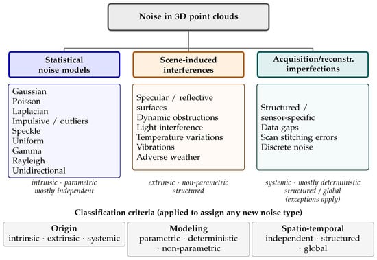
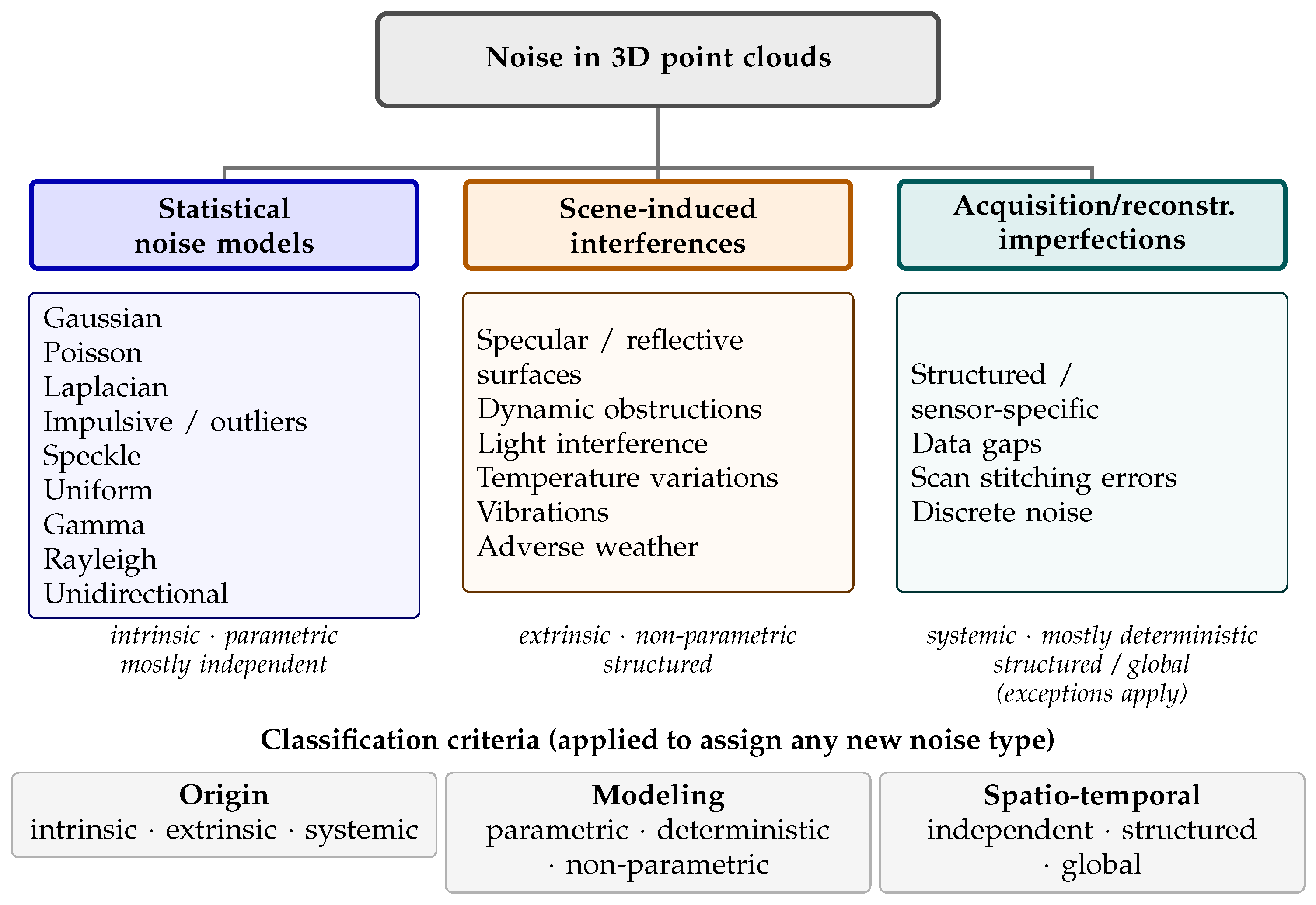

Disclaimer/Publisher’s Note: The statements, opinions and data contained in all publications are solely those of the individual author(s) and contributor(s) and not of MDPI and/or the editor(s). MDPI and/or the editor(s) disclaim responsibility for any injury to people or property resulting from any ideas, methods, instructions or products referred to in the content. |
© 2026 by the authors. Licensee MDPI, Basel, Switzerland. This article is an open access article distributed under the terms and conditions of the Creative Commons Attribution (CC BY) license.