Machine Learning-Assisted Modal Reconstruction of an Aluminum Plate from Vision-Based Deflection Measurements

Abstract

The reconstruction of structural deformation fields from sparse or indirect measurements represents a key challenge in structural health monitoring, particularly for real-time applications involving lightweight mechanical components. In linear elastic systems, any deformation state can be represented as a linear combination of structural mode shapes through modal superposition. Exploiting this property, the present work proposes a machine learning-based framework for the real-time reconstruction of the deflection field of an aluminium plate subjected to the impingement of a non-stationary water flow. The methodology combines modal superposition with a supervised Random Forest classifier trained on a database of known deformation states generated from a finite element model. For each deformation state, the retained modes are selected through a novel linear-regression-based criterion, in which the optimal modal subset is identified by simultaneously promoting a unit regression slope, a vanishing intercept, and a Pearson correlation coefficient close to unity between the reconstructed and reference deflection fields. The proposed strategy is compared with the previously developed Internal Strain Potential Energy Criterion (ISPEC), providing a direct comparison between an energy-based and a reconstruction-oriented mode selection approach. Experimental deflections are acquired through a vision-based displacement tracking system. Seven measurement points, located close to the clamped boundary and therefore far from the fluid excitation, are used as input to the reconstruction algorithm, whereas additional markers positioned closer to the fluid-loaded region are retained exclusively for validation, providing a more demanding assessment of the methodology. The classifier identifies the active modes from the measured deflection pattern, while the full-field structural response is recovered through modal superposition. Experimental validation demonstrates that the proposed regression-based approach consistently improves the reconstruction accuracy with respect to ISPEC. At the most demanding validation point, located closest to the fluid excitation, the mean reconstruction error is approximately $1.65\mathrm{mm}$ for deflection amplitudes reaching $25\mathrm{mm}$, corresponding to an NRMSE of $10.60\%$, compared with $14.74\%$ obtained using ISPEC, representing a reduction of $28.1\%$. Despite this improvement, the average computation time remains below $0.3\mathrm{ms}$, confirming the suitability of the proposed framework for real-time applications. These results demonstrate that the proposed methodology provides an accurate, computationally efficient, and robust solution for real-time full-field deformation estimation from sparse non-contact optical measurements.

1. Introduction

Modal superposition is a well-established method in structural dynamics, based on the linear combination of mode shapes to describe structural displacement or strain fields. It has been widely adopted in engineering applications because it provides a computationally efficient alternative to direct numerical integration methods [1,2,3,4]. Although it is primarily used to evaluate the transient dynamic response of structures [5,6], modal superposition has also found widespread application in other fields, including the analysis of seismic site response [7,8,9].

Beyond these traditional applications, modal superposition provides the theoretical foundation for modal reconstruction, namely the estimation of a full-field structural deformation from a limited number of sparse measurements. Modal reconstruction algorithms recover the displacement field of a structure from measurements available only at a restricted number of locations [10,11,12,13,14,15,16,17,18]. Assuming linear elastic behaviour and small displacements, the structural response can be represented by a reduced set of vibration modes, allowing the complete deformation field to be reconstructed by estimating the corresponding modal coordinates.

This capability is particularly attractive for structural health monitoring (SHM), where measuring the complete structural response is often impractical. Sensors or optical markers can usually be installed only at accessible locations, without interfering with the normal operation of the monitored component. When the modal shapes are available from a finite element (FE) model, the measured displacements at these locations can be used to estimate the modal coordinates and reconstruct the full-field structural response. The resulting displacement and strain fields provide valuable information for damage detection, anomaly identification, and condition assessment of engineering structures.

Modal reconstruction has also been investigated for shape reconstruction from partial displacement or strain measurements [18,19,20,21,22,23,24,25]. Such approaches are particularly relevant for SHM applications, where reliable real-time estimation of structural deformation must often be achieved from a limited number of measurements [26,27]. Furthermore, for isotropic, homogeneous, and linearly elastic structures, reconstructed displacement and strain fields may also be exploited to infer the corresponding stress state through compatibility conditions and constitutive relations, further increasing the value of modal reconstruction for monitoring safety-critical systems.

A fundamental challenge in modal reconstruction is the selection of the vibration modes to be retained [28]. Retaining too few modes may compromise the reconstruction accuracy, whereas including unnecessary or poorly correlated modes may increase computational cost and introduce numerical instability. Consequently, the retained modal basis should be as compact as possible while preserving the capability to reproduce the structural response. Several mode selection criteria have been proposed over the years [29,30]. Among these, energy-based approaches such as the Internal Strain Potential Energy Criterion (ISPEC) have demonstrated the importance of selecting modes according to their physical contribution to the deformation field [31].

In a previous study [32], a modal reconstruction framework was proposed for the structural health monitoring of a flexible aluminium plate subjected to unsteady water-flow excitation. The methodology combined the Internal Strain Potential Energy Criterion (ISPEC) with a Random Forest classifier to enable real-time modal identification from sparse displacement measurements. In that formulation, the modal labels used for supervised learning were generated through an energy-based criterion, whereby the retained modes were selected according to their contribution to the internal strain potential energy. The present work extends this framework by introducing a reconstruction-oriented modal selection criterion. Rather than selecting modes according to their energetic contribution, the proposed approach directly evaluates the quality of the reconstructed displacement field obtained from progressively enlarged modal subsets. The optimal modal basis is therefore selected according to its reconstruction capability, making the selection process explicitly consistent with the final objective of accurately reconstructing the full-field structural deflection from sparse measurements.

For each known deformation state, the available modes are first ranked according to their correlation with the sparse deflection measurements. Candidate modal subsets are then progressively tested by reconstructing the full-field deflection and comparing it with the corresponding finite element solution through linear regression. The optimal subset is identified by simultaneously promoting a Pearson correlation coefficient close to unity, a regression slope close to one, and a negligible regression intercept. The selected modal subsets are subsequently encoded as binary labels and used to train a supervised Random Forest classifier. Once trained, the classifier predicts the active modal subset directly from sparse experimental measurements, allowing the modal coordinates and the corresponding full-field deflection to be reconstructed through modal superposition.

To extend this strategy to real-time SHM applications, the selected modal subsets are encoded as binary labels and used to train a supervised Random Forest classifier. Once trained, the classifier predicts the active modal subset directly from sparse experimental measurements, allowing the modal coordinates and the corresponding full-field deflection to be reconstructed through modal superposition.

The proposed methodology is experimentally validated on a flexible aluminium plate subjected to unsteady water-flow excitation in a closed-loop water tunnel. Plate deflections are measured through a vision-based optical tracking system using only seven marker locations as input to the reconstruction algorithm, while additional markers are retained as independent verification points. Reconstruction accuracy is assessed by comparing the reconstructed and measured deflection histories at the verification markers using root-mean-square error, normalised root-mean-square error, and signal correlation metrics. The reconstruction performance obtained with the proposed regression-based modal selection is also compared with that achieved using the Internal Strain Potential Energy Criterion (ISPEC), allowing the effectiveness of the proposed mode selection strategy to be quantitatively assessed. Finally, the computational performance of the proposed framework is evaluated to assess its suitability for real-time structural health monitoring.

The remainder of the paper is organised as follows. Section 2 describes the experimental setup, including the water tunnel, the aluminium plate, and the optical measurement system. Section 3 presents the proposed methodology, including modal reconstruction, regression-based mode selection, finite element database generation, Random Forest training, and online reconstruction. Section 4 reports and discusses the experimental results. Finally, Section 5 summarises the main conclusions and outlines future developments.

2. Experimental Setup

2.1. Water Tunnel and Optical Acquisition System

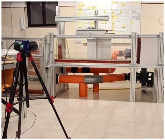
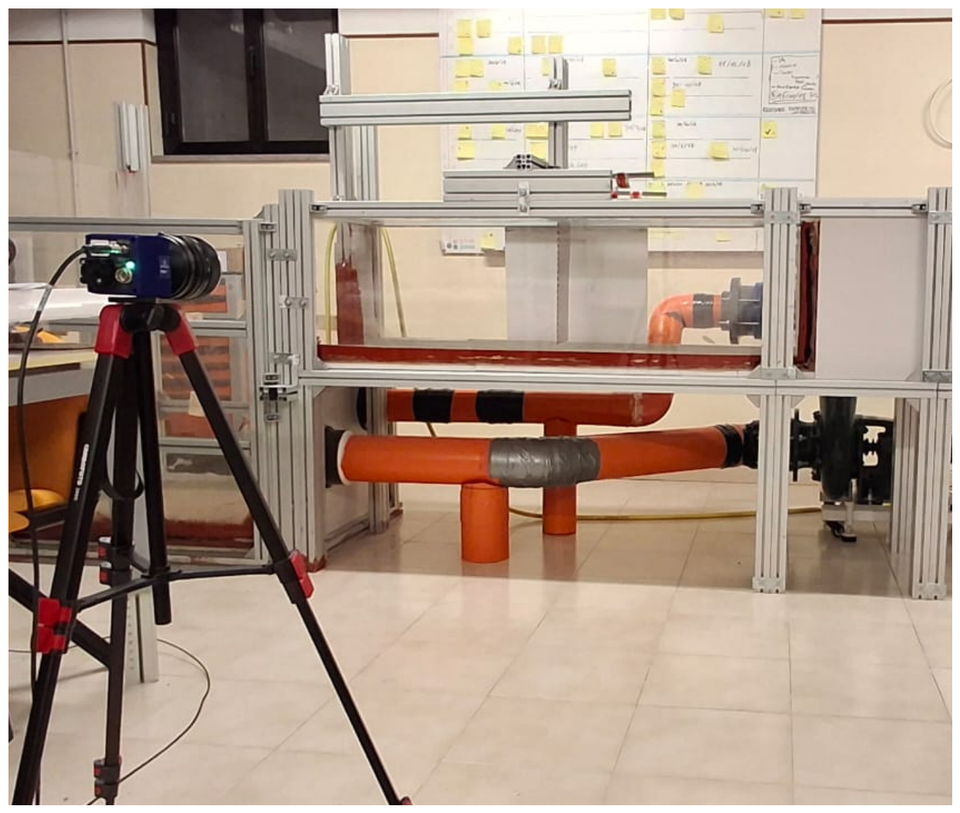
The experiments were carried out in the recirculating closed-loop water tunnel facility at the University of Tuscia. The test section consists of a transparent prismatic chamber with dimensions $1.30\times 0.49\times 0.45{\mathrm{m}}^3$ ($L\times W\times H$), providing full optical access for displacement measurements. The flow is generated by a centrifugal pump driven by an inverter-controlled asynchronous electric motor, allowing the free-stream velocity to be continuously adjusted through the pump rotational speed. Within the investigated operating conditions, the flow velocity ranges from approximately $0.1\mathrm{m}/\mathrm{s}$ to $0.5\mathrm{m}/\mathrm{s}$, corresponding to Reynolds numbers of the order of ${10}^4$. During the experiments, a flexible aluminium plate is vertically mounted inside the test section and subjected to the hydrodynamic loading generated by the unsteady water flow. A general view of the experimental facility, including the water tunnel, the aluminium plate, and the optical acquisition system, is shown in Figure 1.

Figure 1. General overview of the water tunnel facility, showing the test section, the aluminium plate, and the optical acquisition system.

The optical acquisition system consists of a high-resolution CMOS camera used for marker tracking. The camera has a sensor resolution of $2440\times 2040$ pixels and acquires images at $123\mathrm{fps}$ at full resolution. The proposed reconstruction procedure does not identify vibration modes from the temporal frequency content of the measured signals. Instead, each acquired frame is processed independently: the instantaneous deflections measured at the seven input markers define the spatial deformation pattern supplied to the Random Forest classifier, which identifies the FE mode shapes required for its reconstruction. The FE mode shapes therefore act as spatial basis functions rather than as experimentally identified oscillations at their corresponding natural frequencies. Consequently, the acquisition frequency determines the temporal resolution of the monitored deformation history, while the modal reconstruction itself is based on the instantaneous spatial configuration measured at each frame. The camera is equipped with a fixed focal length lens and is positioned laterally with respect to the test section in order to capture the out-of-plane motion of the plate. Illumination is provided by an LED light source producing a collimated light sheet.

2.2. Aluminium Plate and Marker Layout

The monitored structure is a flexible aluminium plate with dimensions $200\mathrm{mm}\times 400\mathrm{mm}\times 2.5\mathrm{mm}$. The plate is vertically mounted inside the water tunnel test section, with its upper edge clamped to produce a fixed-free boundary condition. The lower portion is immersed in water and directly exposed to the unsteady flow, while the upper portion remains above the free surface and visible to the optical acquisition system.

The structural quantity of interest is the plate deflection, denoted by $\eta$, defined as the displacement component orthogonal to the plate mid-plane. High-contrast reflective markers are applied along the longitudinal edge visible to the camera. They are equally spaced by $20\mathrm{mm}$, starting from the clamped edge and extending towards the free surface.

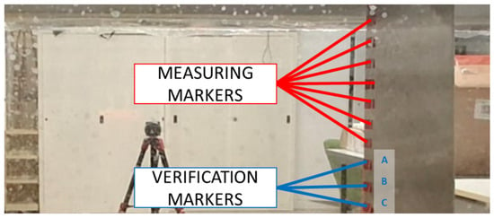
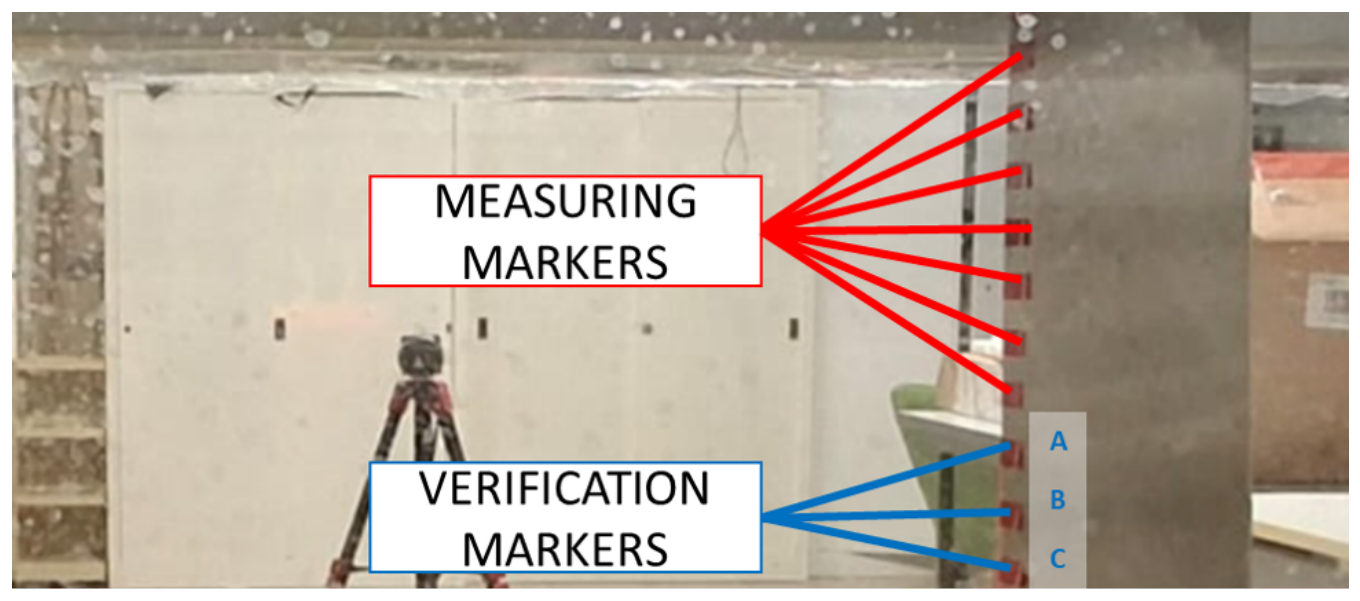
The first seven visible markers, located closest to the clamped boundary, provide the sparse deflection vector used as input to the reconstruction algorithm. These are shown in Figure 2. The three subsequent markers are excluded from the reconstruction and retained as independent verification points. This configuration provides a deliberately demanding validation, since measurements are acquired closer to the constraint, where deflections are smaller and farther from the fluid loading, whereas reconstruction is verified progressively closer to the fluid-excited region, where larger deflections occur.

Figure 2. Marker layout used for image-based displacement tracking.

The marker locations are prescribed rather than optimised, reflecting practical monitoring conditions in which measurement positions are constrained by accessibility, visibility, and installation requirements. Their spatial distribution can nevertheless affect modal selection, since the modal coordinates depend on the mode-shape values at the measurement locations. The regression-based criterion therefore identifies the modal subset providing the best reconstruction for the prescribed marker configuration. Figure 3 and Figure 4 refer specifically to this deliberately demanding measurement layout.

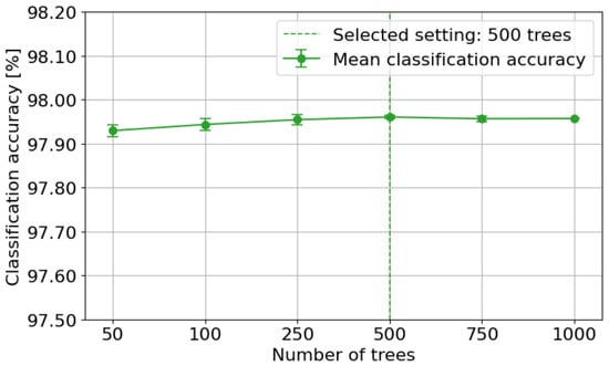
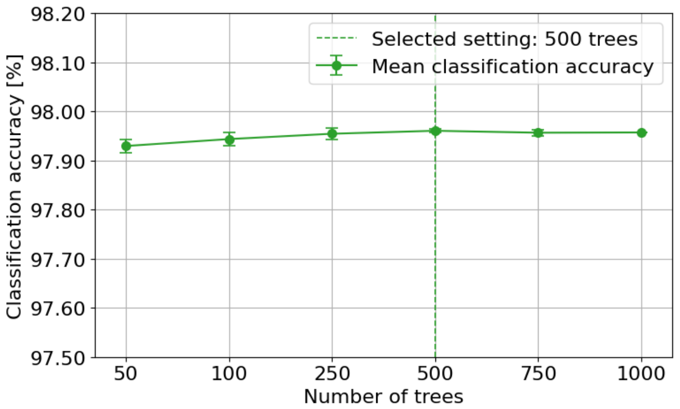
Figure 3. Sensitivity of the Random Forest classifier associated with the proposed regression-based modal selection procedure to the number of trees. Markers represent the mean classification accuracy obtained from five random initialisations, while the error bars indicate the corresponding standard deviation. The dashed vertical line identifies the adopted configuration of 500 trees.

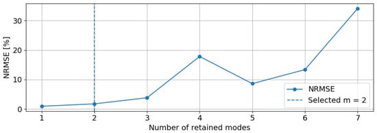
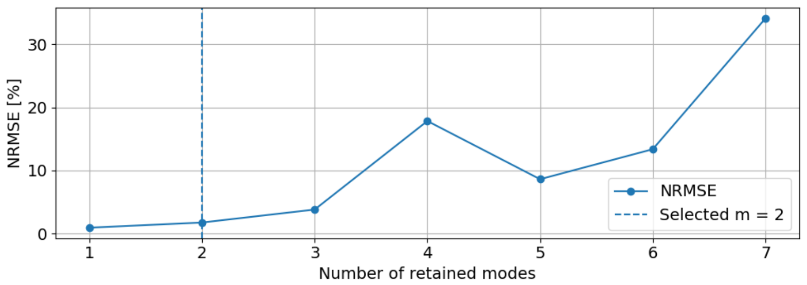
Figure 4. NRMSE as a function of the number of retained modes for the selected finite element case. The vertical dashed line indicates the number of modes selected by the regression-based score, $m=2$.

The number of input markers was selected considering both the optically accessible plate geometry and the requirements of the modal inversion. Seven input measurements allow up to seven modal coordinates to be estimated without producing an underdetermined system. Since the selection procedure generally retains fewer than seven modes, the modal-coordinate estimation is typically overdetermined. Increasing the number of independent measurement locations can provide additional spatial information, whereas reducing their number requires a corresponding limitation of the number of simultaneously retained modes. The marker distribution must also provide sufficiently independent information on the retained mode shapes to ensure stable modal-coordinate estimation.

3. Methodology

3.1. Measurement Selection and Deflection Notation

The proposed methodology reconstructs the full-field deflection of the plate from sparse optical measurements. The monitored quantity is the scalar deflection field $\eta$, corresponding to the displacement component orthogonal to the plate mid-plane. At each time instant t, the full-field deflection vector is written as

$$\eta \left(t\right)={\left[{\eta }_1\left(t\right),{\eta }_2\left(t\right),\dots ,{\eta }_{N_n}\left(t\right)\right]}^T$$

(1)

where $N_n$ is the number of nodes or spatial points used to describe the plate deflection field.

Only a limited number of marker deflections is experimentally measured. Let $N_s$ be the number of input markers used by the reconstruction algorithm. In the present implementation,

$$N_s=7$$

(2)

The corresponding sparse measurement vector is

$${\eta }_s\left(t\right)={\left[{\eta }_{s,1}\left(t\right),{\eta }_{s,2}\left(t\right),\dots ,{\eta }_{s,N_s}\left(t\right)\right]}^T$$

(3)

Since one deflection component is measured at each marker, the number of independent measurement equations coincides with the number of input markers. The remaining visible markers are used only for verification and are excluded from the modal inversion.

3.2. Modal Reconstruction of the Plate Deflection

The modal reconstruction procedure is based on the assumption that the plate behaves within the linear elastic range and that small displacements occur. Under these hypotheses, the instantaneous deflection field can be represented as a linear combination of vibration mode shapes:

$$\eta \left(t\right)=\varphi ·\mu \left(t\right)$$

(4)

where $\eta \left(t\right)$ is the full-field deflection vector, $\varphi$ is the modal matrix, and $\mu \left(t\right)$ is the vector of modal coordinates. The modal matrix is defined as

$$\varphi =\left[{\varphi }_1,{\varphi }_2,\dots ,{\varphi }_{N_m}\right]$$

(5)

where ${\varphi }_i$ is the i-th modal deflection shape and $N_m$ is the number of available modes. The vector of modal coordinates is

$$\mu \left(t\right)={\left[{\mu }_1\left(t\right),{\mu }_2\left(t\right),\dots ,{\mu }_{N_m}\left(t\right)\right]}^T$$

(6)

In practice, the modal coordinates cannot be directly obtained from the full-field deflection vector because only the marker deflections are measured. Therefore, Equation (4) is restricted to the measurement locations:

$${\eta }_s\left(t\right)={\varphi }_s·\mu \left(t\right)$$

(7)

where ${\varphi }_s$ is the modal matrix evaluated only at the marker locations used as input.

If a reduced set of modes is retained, the sparse modal relation becomes

$${\eta }_s\left(t\right)={\varphi }_{s,r}·{\mu }_r\left(t\right)$$

(8)

where ${\varphi }_{s,r}$ contains only the retained modal columns and ${\mu }_r\left(t\right)$ is the corresponding reduced vector of modal coordinates.

For an overdetermined or exactly determined system, the modal coordinates are computed in the least-squares sense as

$${\mu }_r\left(t\right)={\left({\varphi }_{s,r}^T·{\varphi }_{s,r}\right)}^{-1}·{\varphi }_{s,r}^T·{\eta }_s\left(t\right)$$

(9)

More generally, the same operation can be expressed through the Moore–Penrose pseudo-inverse:

$${\mu }_r\left(t\right)={\varphi }_{s,r}^{+}·{\eta }_s\left(t\right)$$

(10)

Once the reduced modal coordinates have been computed, the full-field plate deflection is reconstructed as

$${\eta }_{rec}\left(t\right)={\varphi }_r·{\mu }_r\left(t\right)$$

(11)

where ${\varphi }_r$ is the full-field modal matrix containing the same retained modes used in the sparse inversion.

The modal reconstruction is well posed only if the number of independent measurement equations is greater than or equal to the number of retained modes. Therefore, the following condition is imposed:

$$N_s\ge N_r$$

(12)

where $N_r$ is the number of retained modes. Since one deflection component is measured at each of the seven input markers, the maximum number of retained modes is constrained by

$$N_r\le 7$$

(13)

This constraint avoids an underdetermined modal inversion and reduces the risk of unstable reconstructions.

3.3. Regression-Based Mode Selection

The accuracy of the modal reconstruction depends on the subset of vibration modes retained in the reduced modal matrix. Retaining too few modes may not be sufficient to reproduce the actual deflection field, while retaining modes that are weakly related to the measured deformation may increase the reconstruction error. A regression-based mode selection criterion is therefore introduced to identify, for each known deflection state, the modal subset that provides the best agreement between the reconstructed full-field deflection and the corresponding reference deflection.

Let ${\eta }^{\left(j\right)}$ be the reference full-field deflection vector associated with the j-th known deformation state:

$${\eta }^{\left(j\right)}={\left[{\eta }_1^{\left(j\right)},{\eta }_2^{\left(j\right)},\dots ,{\eta }_{N_n}^{\left(j\right)}\right]}^T$$

(14)

and let the corresponding sparse deflection vector be

$${\eta }_s^{\left(j\right)}={\left[{\eta }_{s,1}^{\left(j\right)},{\eta }_{s,2}^{\left(j\right)},\dots ,{\eta }_{s,N_s}^{\left(j\right)}\right]}^T$$

(15)

For each mode i, the Pearson correlation coefficient between the sparse modal shape ${\varphi }_{s,i}$ and the sparse reference deflection ${\eta }_s^{\left(j\right)}$ is computed. The mean values are

$${\overline{\varphi }}_{s,i}={\displaystyle \frac{1}{N_s}}{\displaystyle \sum _{k=1}^{N_s}}{\varphi }_{s,i,k}$$

(16)

and

$${\overline{\eta }}_s^{\left(j\right)}={\displaystyle \frac{1}{N_s}}{\displaystyle \sum _{k=1}^{N_s}}{\eta }_{s,k}^{\left(j\right)}$$

(17)

The Pearson coefficient is then

$${\rho }_i^{\left(j\right)}={\displaystyle \frac{{\sum }_{k=1}^{N_s}\left({\varphi }_{s,i,k}-{\overline{\varphi }}_{s,i}\right)·\left({\eta }_{s,k}^{\left(j\right)}-{\overline{\eta }}_s^{\left(j\right)}\right)}{\sqrt{{\sum }_{k=1}^{N_s}{\left({\varphi }_{s,i,k}-{\overline{\varphi }}_{s,i}\right)}^2}·\sqrt{{\sum }_{k=1}^{N_s}{\left({\eta }_{s,k}^{\left(j\right)}-{\overline{\eta }}_s^{\left(j\right)}\right)}^2}}}$$

(18)

This coefficient ranges between $-1$ and 1 and measures the similarity between the measured sparse deflection shape and each modal shape evaluated at the same locations.

Since a mode may contribute to the deflection field with either a positive or a negative modal coordinate, the modes are sorted according to the absolute value of the correlation coefficient:

$$\left|{\rho }_{i_1}^{\left(j\right)}\right|\ge \left|{\rho }_{i_2}^{\left(j\right)}\right|\ge \cdots \ge \left|{\rho }_{i_{N_m}}^{\left(j\right)}\right|$$

(19)

For a given number of retained modes r, the candidate modal subset is

$$M_r^{\left(j\right)}=\left[i_1,i_2,\dots ,i_r\right],r=1,2,\dots ,r_{max}$$

(20)

The maximum number of retained modes is

$$r_{max}=\min \left(N_s,N_m\right)$$

(21)

For each candidate subset, the modal coordinates are obtained from the sparse reference deflection through pseudo-inverse-based inversion:

$${\mu }_r^{\left(j\right)}={\left({\varphi }_{s,r}^{\left(j\right)}\right)}^{+}·{\eta }_s^{\left(j\right)}$$

(22)

The corresponding full-field reconstruction is

$${\eta }_{rec,r}^{\left(j\right)}={\varphi }_r^{\left(j\right)}·{\mu }_r^{\left(j\right)}$$

(23)

The quality of the candidate reconstruction is evaluated by comparing ${\eta }_{rec,r}^{\left(j\right)}$ with the known full-field reference deflection ${\eta }^{\left(j\right)}$. The comparison is performed through the linear regression model

$${\eta }_{rec,r}^{\left(j\right)}={\alpha }_{1,r}^{\left(j\right)}·{\eta }^{\left(j\right)}+{\alpha }_{0,r}^{\left(j\right)}·1$$

(24)

where 1 is a vector of ones, ${\alpha }_{1,r}^{\left(j\right)}$ is the regression slope, and ${\alpha }_{0,r}^{\left(j\right)}$ is the regression intercept. A perfect reconstruction gives

$${\alpha }_{1,r}^{\left(j\right)}=1,{\alpha }_{0,r}^{\left(j\right)}=0$$

(25)

The mean values of the reference and reconstructed deflection fields are

$${\overline{\eta }}^{\left(j\right)}={\displaystyle \frac{1}{N_n}}{\displaystyle \sum _{k=1}^{N_n}}{\eta }_k^{\left(j\right)}$$

(26)

and

$${\overline{\eta }}_{rec,r}^{\left(j\right)}={\displaystyle \frac{1}{N_n}}{\displaystyle \sum _{k=1}^{N_n}}{\eta }_{rec,r,k}^{\left(j\right)}$$

(27)

The regression slope is computed as

$${\alpha }_{1,r}^{\left(j\right)}={\displaystyle \frac{{\sum }_{k=1}^{N_n}\left({\eta }_k^{\left(j\right)}-{\overline{\eta }}^{\left(j\right)}\right)·\left({\eta }_{rec,r,k}^{\left(j\right)}-{\overline{\eta }}_{rec,r}^{\left(j\right)}\right)}{{\sum }_{k=1}^{N_n}{\left({\eta }_k^{\left(j\right)}-{\overline{\eta }}^{\left(j\right)}\right)}^2}}$$

(28)

Once the slope has been computed, the intercept is obtained as

$${\alpha }_{0,r}^{\left(j\right)}={\overline{\eta }}_{rec,r}^{\left(j\right)}-{\alpha }_{1,r}^{\left(j\right)}·{\overline{\eta }}^{\left(j\right)}$$

(29)

The slope measures the amplitude consistency between reconstructed and reference fields, while the intercept quantifies the offset between them.

In addition, the Pearson correlation coefficient between the full-field reference deflection and the reconstructed deflection is computed as

$$R_r^{\left(j\right)}={\displaystyle \frac{{\sum }_{k=1}^{N_n}\left({\eta }_k^{\left(j\right)}-{\overline{\eta }}^{\left(j\right)}\right)·\left({\eta }_{rec,r,k}^{\left(j\right)}-{\overline{\eta }}_{rec,r}^{\left(j\right)}\right)}{\sqrt{{\sum }_{k=1}^{N_n}{\left({\eta }_k^{\left(j\right)}-{\overline{\eta }}^{\left(j\right)}\right)}^2}·\sqrt{{\sum }_{k=1}^{N_n}{\left({\eta }_{rec,r,k}^{\left(j\right)}-{\overline{\eta }}_{rec,r}^{\left(j\right)}\right)}^2}}}$$

(30)

The coefficient $R_r^{\left(j\right)}$ evaluates the similarity between the spatial shape of the reconstructed deflection and the reference deflection.

The optimal number of retained modes is selected by combining three indicators: the full-field correlation coefficient $R_r^{\left(j\right)}$, the slope error $\left|{\alpha }_{1,r}^{\left(j\right)}-1\right|$, and the intercept error $\left|{\alpha }_{0,r}^{\left(j\right)}\right|$. Each quantity is converted into a normalised score between 0 and 1:

$$s_{R,r}^{\left(j\right)}={\displaystyle \frac{R_r^{\left(j\right)}-{\min }_{\mathsf{\ell }}{R}_{\mathsf{\ell }}^{\left(j\right)}}{{\max }_{\mathsf{\ell }}{R}_{\mathsf{\ell }}^{\left(j\right)}-{\min }_{\mathsf{\ell }}{R}_{\mathsf{\ell }}^{\left(j\right)}}},\mathsf{\ell }=1,\dots ,r_{max}$$

(31)

$$s_{{\alpha }_1,r}^{\left(j\right)}=1-{\displaystyle \frac{\left|{\alpha }_{1,r}^{\left(j\right)}-1\right|}{{\max }_{\mathsf{\ell }}\left|{\alpha }_{1,\mathsf{\ell }}^{\left(j\right)}-1\right|}}$$

(32)

and

$$s_{{\alpha }_0,r}^{\left(j\right)}=1-{\displaystyle \frac{\left|{\alpha }_{0,r}^{\left(j\right)}\right|}{{\max }_{\mathsf{\ell }}\left|{\alpha }_{0,\mathsf{\ell }}^{\left(j\right)}\right|}}$$

(33)

If the denominator of one of the normalised scores is zero, that score is set equal to one for all candidate reconstructions, since the corresponding indicator does not distinguish between the tested modal subsets.

The total score is defined as

$$S_r^{\left(j\right)}={\displaystyle \frac{s_{R,r}^{\left(j\right)}+s_{{\alpha }_1,r}^{\left(j\right)}+s_{{\alpha }_0,r}^{\left(j\right)}}{3}}·100$$

(34)

The best modal subset is the one that maximises this score:

$$r^{*\left(j\right)}=arg\underset{r}{\max }{S}_r^{\left(j\right)}$$

(35)

and therefore

$$M^{*\left(j\right)}=M_{r^{*\left(j\right)}}^{\left(j\right)}$$

(36)

The selected reconstruction is finally written as

$${\eta }_{rec}^{\left(j\right)}={\eta }_{rec,r^{*}}^{\left(j\right)}$$

(37)

Its error is quantified through the root-mean-square error:

$$RMS{E}^{\left(j\right)}=\sqrt{{\displaystyle \frac{1}{N_n}}\sum _{k=1}^{N_n}{\left({\eta }_{rec,k}^{\left(j\right)}-{\eta }_k^{\left(j\right)}\right)}^2}$$

(38)

and the normalised root-mean-square error:

$$NRMS{E}^{\left(j\right)}[\%]=100·{\displaystyle \frac{RMS{E}^{\left(j\right)}}{{\max }_k\left({\eta }_k^{\left(j\right)}\right)-{\min }_k\left({\eta }_k^{\left(j\right)}\right)}}$$

(39)

Only the deformation states satisfying

$$NRMS{E}^{\left(j\right)}\le NRMS{E}_{max}$$

(40)

are retained in the final training database. The selected modal subset is then encoded into a binary vector:

$$y_i^{\left(j\right)}=\left\{\begin{array}{cc}1,\hfill & \mathrm{if}i\in M^{*\left(j\right)},\hfill \\ 0,\hfill & \mathrm{otherwise}.\hfill \end{array}\right.$$

(41)

This binary vector represents the target output used to train the Random Forest classifier.

3.4. Finite Element Model and Database Generation

A finite element model of the aluminium plate is developed to reproduce the geometry and boundary conditions of the experimental specimen. The model is developed in ANSYS Mechanical APDL 2020 R2 using SOLID185 linear structural solid elements [33]. A mapped mesh of 12800 hexahedral elements is adopted, with four elements through the $2.5\mathrm{mm}$ plate thickness to adequately represent the bending deformation. The experimentally clamped edge is modelled by constraining its translational degrees of freedom, providing a suitable kinematic approximation of the fixed-free experimental configuration. Although the local compliance of the actual clamp is not explicitly represented and may affect the natural frequencies, the FE mode shapes are used as spatial basis functions rather than for direct numerical–experimental frequency matching. Their suitability is ultimately assessed through reconstruction at independent experimental verification locations.

The FE model serves two purposes: a modal analysis provides the candidate mode shapes for reconstruction, while a structural transient analysis generates the deformation database used for supervised learning.

The FE model is not intended to reproduce the experimental fluid–structure interaction. The natural frequencies associated with the FE mode shapes are not used as inputs to the reconstruction algorithm, and no direct correspondence with the experimental natural frequencies is required. Similarly, the transient analysis does not reproduce the specific deformation history induced by the water flow, but provides a sufficiently large set of known deformation states for training. Consequently, fluid added-mass effects are not included, as they would be required for reproducing the coupled dynamic response rather than for generating the spatial reconstruction basis and training states.

The transient simulation is performed by applying a time-dependent force along the deflection direction to the nodes located at the free edge of the plate according to

$$F\left(t\right)=F_{0}cos\left(\omega t\right)$$

(42)

where

$$F_0=50\mathrm{N}$$

(43)

and

$$\omega =2\pi f,f=50\mathrm{Hz}$$

(44)

The $50\mathrm{Hz}$ excitation is a numerical parameter used to generate time-varying deformation states and is not intended to reproduce the experimental fluid excitation. The load is applied for $50\mathrm{s}$, followed by $2\mathrm{s}$ of free oscillation, thereby providing deformation states from both forced and free responses.

The transient integration time step is selected according to the highest natural frequency included in the candidate modal basis. Since the first 50 mode shapes are considered, it is defined as

$$\Delta t={\displaystyle \frac{1}{20f_{\max }}}$$

(45)

where $f_{\max }$ is the natural frequency associated with the 50th mode. This provides 20 integration points over the corresponding period and adequately resolves the highest-frequency contribution included in the candidate basis.

The transient analysis provides a sequence of full-field deflection states. At each stored instant $t_j$, the nodal deflection vector is

$${\eta }^{\left(j\right)}=\eta \left(t_j\right),j=1,2,\dots ,N_t$$

(46)

The integration time step should not be confused with the sampling of the training database. The complete transient response is integrated using the prescribed time step, while only 15,000 deformation states are retained for computational storage reasons. These states are used as independent machine learning samples without modifying the temporal discretisation of the FE solution.

The database therefore contains

$$N_t=15,000$$

(47)

stored deformation states.

Each stored state is treated as an independent training case. For the j-th snapshot, ${\eta }^{\left(j\right)}$ represents the known full-field deformation, while the corresponding sparse vector ${\eta }_s^{\left(j\right)}$ contains the deflections at the same seven locations used as experimental inputs. The regression-based procedure independently selects, among the 50 candidate modes, the subset providing the most suitable reconstruction from these sparse values and generates the corresponding binary label.

The numerical excitation therefore does not directly prescribe the modes contained in the training labels. Instead, the Random Forest learns the relationship between sparse deformation patterns and the modal subsets required for their reconstruction. Different numerical excitation parameters may alter the distribution of deformation states in the database, but they are not required to reproduce the experimental loading, since each stored state is independently evaluated according to its reconstruction capability.

3.5. Random Forest Classifier for Modal Identification

The modal identification problem is formulated as a multi-label classification task. Each training sample is composed of the sparse deflection values extracted at the seven input marker locations, while the corresponding target is the binary vector identifying the modes selected by the regression-based procedure. Therefore, the classifier learns the relation between the measured deflection pattern and the modal subset required for reconstruction.

The Random Forest classifier was implemented using the RandomForestClassifier algorithm. The main settings used in the present work are reported in Table 1. The model consists of 500 decision trees and uses bootstrap aggregation. The Gini impurity criterion is adopted for node splitting. No maximum tree depth is imposed, so each tree is expanded until the default stopping criteria are reached. The minimum number of samples required to split an internal node is set to 2, while the minimum number of samples in a terminal leaf is set to 1. At each split, the number of candidate input features is set equal to the square root of the total number of features. No class weighting is applied. A fixed random seed equal to 1 is used to ensure reproducibility, and all available CPU cores are used for parallel computation.

Table 1. Random Forest settings used for modal subset prediction.

Setting	Value
Classifier	RandomForestClassifier
Number of trees	500
Splitting criterion	Gini impurity
Maximum depth	None
Minimum samples for split	2
Minimum samples per leaf	1
Features per split	Square root
Bootstrap sampling	True
Class weighting	None
Random seed	1
Parallel jobs	$-1$
Number of modal classes	50
Input features	7 marker deflections

A sensitivity analysis was performed to assess the influence of the number of trees on the classifier performance associated with the proposed regression-based modal selection procedure. Random Forest ensembles composed of 50, 100, 250, 500, 750, and 1000 trees were tested while keeping all other hyperparameters unchanged. For each ensemble size, five different random seeds (1–5) were considered using the same fixed training and test datasets. The use of multiple seeds was limited to the sensitivity analysis in order to quantify the variability associated with the stochastic construction of the Random Forest. The final classifier employed for the experimental reconstruction was instead trained using the fixed seed reported in Table 1, i.e., random_state = 1, to ensure reproducibility. Classification performance was evaluated as the percentage of correctly predicted binary modal labels over all samples and modal classes.

As shown in Figure 3, the mean classification accuracy progressively increases from $97.929\%$ for 50 trees to $97.960\%$ for 500 trees. The 500-tree configuration provides the highest mean accuracy among the investigated ensemble sizes, with a standard deviation of only $0.0038\%$ over the five random initialisations. Increasing the ensemble size beyond 500 trees does not provide any further improvement, with mean accuracies of $97.956\%$ and $97.957\%$ obtained for 750 and 1000 trees, respectively. In particular, the difference between the mean accuracies obtained with 500 and 1000 trees is only $0.0034$ percentage points. These results show that the classification performance reaches a stable region at approximately 500 trees and becomes essentially insensitive to a further increase in the ensemble size. Therefore, 500 estimators were retained for the final classifier, providing stable and reproducible classification performance without unnecessarily increasing the computational cost.

After training, the classifier is applied to the experimental deflection measurements on a timestep-by-timestep basis. For each time instant, the seven measured marker deflections are provided as input, and the classifier returns the predicted set of active modes. If no mode is predicted at a given timestep, the most frequently selected mode in the training database is assigned to avoid a null reconstruction.

3.6. Validation Metrics

The reconstructed deflection is validated by comparing the reconstructed signals with the measured deflections at the markers not used as input [34]. Let ${\eta }_i^{meas}\left(t\right)$ and ${\eta }_i^{rec}\left(t\right)$ be the measured and reconstructed deflections at the i-th verification marker. The instantaneous residual is defined as

$$e_i\left(t\right)={\eta }_i^{rec}\left(t\right)-{\eta }_i^{meas}\left(t\right)$$

(48)

The root-mean-square error over a time window containing $N_t$ samples is

$$RMS{E}_i=\sqrt{{\displaystyle \frac{1}{N_t}}\sum _{k=1}^{N_t}{e}_i^2\left(t_k\right)}$$

(49)

The normalised root-mean-square error is

$$NRMS{E}_i[\%]=100·{\displaystyle \frac{RMS{E}_i}{{\max }_k\left({\eta }_i^{meas}\left(t_k\right)\right)-{\min }_k\left({\eta }_i^{meas}\left(t_k\right)\right)}}$$

(50)

In addition, the normalised cross-correlation is used to evaluate the similarity between measured and reconstructed signals:

$$C{C}_{norm,i}={\displaystyle \frac{{\sum }_{k=1}^{N_t}\left({\eta }_i^{meas}\left(t_k\right)-{\overline{\eta }}_i^{meas}\right)·\left({\eta }_i^{rec}\left(t_k\right)-{\overline{\eta }}_i^{rec}\right)}{\sqrt{{\sum }_{k=1}^{N_t}{\left({\eta }_i^{meas}\left(t_k\right)-{\overline{\eta }}_i^{meas}\right)}^2}·\sqrt{{\sum }_{k=1}^{N_t}{\left({\eta }_i^{rec}\left(t_k\right)-{\overline{\eta }}_i^{rec}\right)}^2}}}$$

(51)

Values of $C{C}_{norm,i}$ close to one indicate strong agreement between measured and reconstructed deflections in terms of waveform similarity.

The computational time required for the reconstruction is also evaluated at each timestep. This includes modal subset identification, computation of the modal coordinates, and reconstruction of the full-field deflection. This metric is essential for assessing the suitability of the proposed procedure for real-time structural health monitoring applications.

4. Results

The performance of the proposed framework is evaluated in three steps. First, the regression-based modal selection procedure is analysed on a representative deformation state extracted from the finite element database. Second, the modal subsets predicted during experimental monitoring are examined. Finally, the complete reconstruction procedure is validated using the measured deflections at three verification markers that were not used as input to the algorithm.

4.1. Example of Regression-Based Modal Selection

A representative case from the finite element database, corresponding to load case 2753, was selected to illustrate the behaviour of the regression-based modal selection procedure. The purpose of this example is to show how the proposed criterion identifies a compact modal subset starting from the sparse deflection values evaluated at the seven input marker locations.

For this deformation state, the available modes were first ranked according to the absolute value of the Pearson correlation coefficient between each mode shape, restricted to the input marker locations, and the corresponding sparse deflection vector. Starting from this ordered list, increasingly larger modal subsets were tested. The number of retained modes was varied from one to seven, consistently with the number of input markers. For each candidate subset, the modal coordinates were estimated from the sparse deflection vector, the full-field deflection was reconstructed by modal superposition, and the reconstructed field was compared with the reference finite element deflection field.

Figure 4 shows the NRMSE obtained for each candidate number of retained modes. The selected modal subset corresponds to $m=2$. The curve highlights that increasing the number of modes does not necessarily improve the reconstruction. In this example, low error values are obtained using a small number of modes, whereas the inclusion of additional modes leads to a marked increase in reconstruction error for several candidate subsets. This confirms that the modal basis must be selected according to the actual deformation state rather than by retaining the largest possible number of modes.

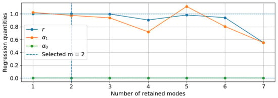
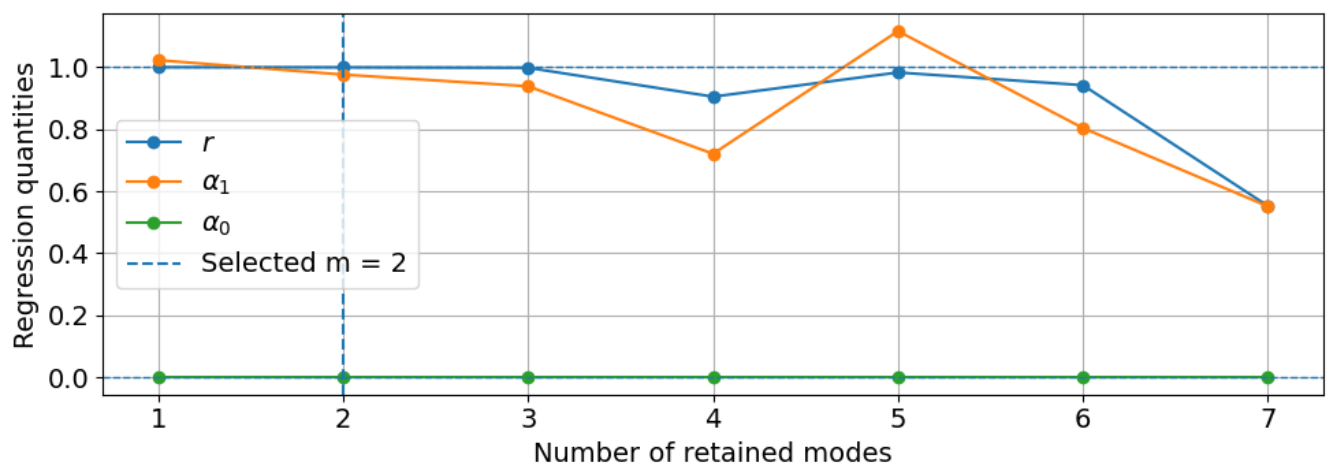
The regression indicators used to define the selection score are reported in Figure 5. The coefficient r represents the Pearson correlation between the reference and reconstructed full-field deflection vectors. Values close to unity indicate that the reconstructed field correctly reproduces the spatial shape of the reference deformation. The coefficient ${\alpha }_1$ is the slope of the regression line and measures the consistency of the reconstructed amplitude, while ${\alpha }_0$ is the intercept and quantifies any systematic offset.

Figure 5. Regression indicators for the selected finite element case. The plot reports the full-field correlation coefficient r, the regression slope ${\alpha }_1$, and the intercept ${\alpha }_0$ as functions of the number of retained modes.

For the analysed case, the selected solution with $m=2$ provides a favourable compromise among the three quantities: high correlation, slope close to unity, and negligible intercept. Although the NRMSE alone is useful for evaluating the reconstruction error, the proposed selection is based on the combined regression score, which simultaneously accounts for spatial similarity, amplitude consistency, and offset reduction.

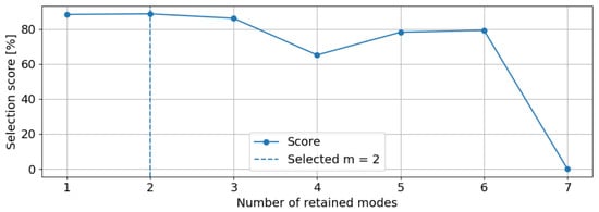
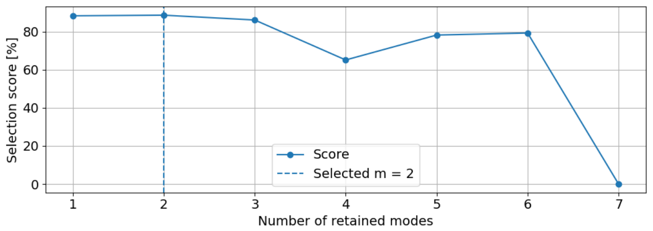
Figure 6 shows the total selection score obtained by combining the normalised contributions associated with the full-field correlation coefficient, the slope error, and the intercept error. The maximum value of the score is obtained for $m=2$, which is therefore selected as the optimal number of retained modes for this deformation state. The score decreases when additional modes are introduced, showing that larger modal subsets do not necessarily provide a better global agreement with the reference field.

Figure 6. Regression-based selection score for the selected finite element case. The highest score is obtained for $m=2$, corresponding to the selected modal subset.

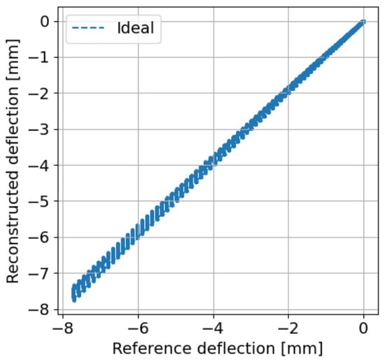
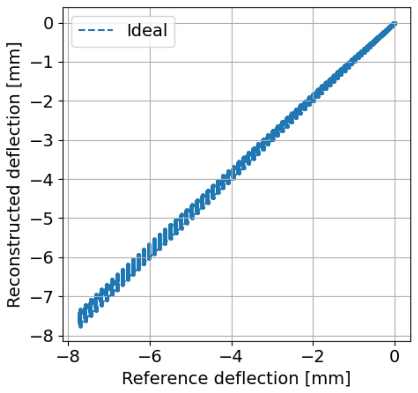
The quality of the selected reconstruction is further assessed in Figure 7, where the reconstructed deflection is plotted against the reference finite element deflection over all nodes. The points are closely aligned with the ideal (1:1) line, confirming that the selected modal subset accurately reproduces both the spatial distribution and the amplitude of the reference deflection field. This result is particularly relevant because the modal coordinates are computed only from the seven sparse marker deflections, whereas the validation is performed over the full finite element field.

Figure 7. Full-field reconstructed deflection versus reference finite element deflection for the selected case. The dashed line represents the ideal reconstruction.

4.2. Modal Selection During Experimental Monitoring

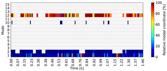
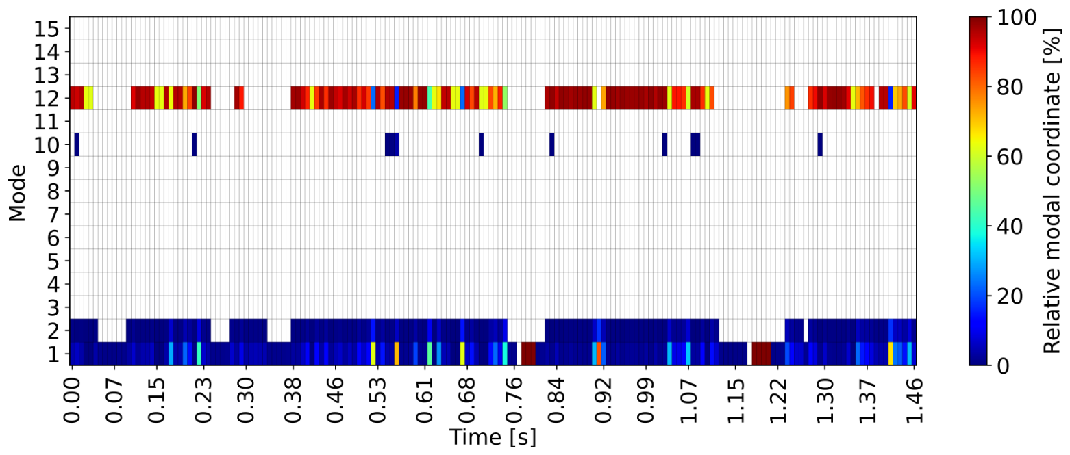
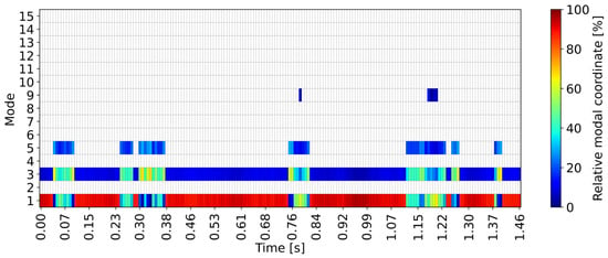
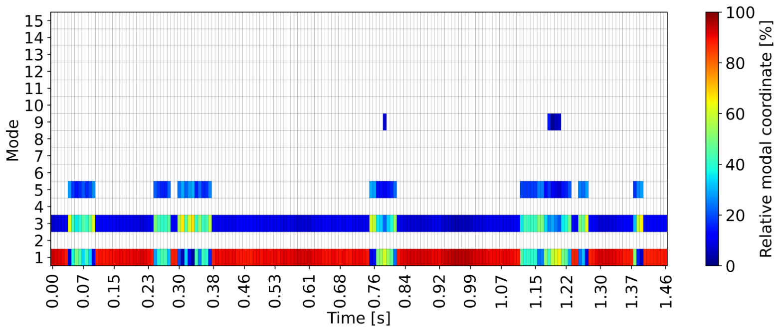
After training, the Random Forest classifier based on the proposed regression-based modal selection criterion was applied to the experimental marker measurements on a timestep-by-timestep basis. For each frame, the classifier received the seven input marker deflections and predicted the corresponding set of active modes. The resulting modal map is shown in Figure 8. For comparison, Figure 9 reports the modal subsets predicted by an equivalent Random Forest classifier trained using ISPEC.

Figure 8. Modal subsets predicted during the experimental monitoring window by the Random Forest classifier trained on the database generated using the proposed regression-based modal selection criterion. The colour scale represents the relative modal-coordinate magnitude $I_i\left(t\right)$, calculated from the experimental measurements according to Equation (52). White cells indicate modes that are not retained at the corresponding timestep.

Figure 9. Modal subsets predicted during the experimental monitoring window by the Random Forest classifier trained on the database generated using ISPEC. The colour scale represents the relative modal-coordinate magnitude $I_i\left(t\right)$, calculated from the experimental measurements according to Equation (52). White cells indicate modes that are not retained at the corresponding timestep.

To provide information on the relative importance of the modes retained by the two classifiers, the modal coordinates calculated from the experimental measurements were also considered. At each timestep t, after identifying the active modal subset $\mathcal{M}\left(t\right)$, the corresponding modal-coordinate vector is obtained according to Equation (10).

The relative magnitude associated with the i-th retained mode is then defined as

$$I_i\left(t\right)={\displaystyle \frac{|{\mu }_i\left(t\right)|}{{\displaystyle \sum _{j\in \mathcal{M}\left(t\right)}\left|{\mu }_j\left(t\right)\right|}}}·100$$

(52)

Accordingly, $I_i\left(t\right)$ expresses the magnitude of each modal coordinate as a percentage of the total modal-coordinate magnitude at the same timestep. This quantity is used only to compare the relative weights of the modes within each instantaneous reconstruction and should not be interpreted as a modal energy contribution.

Both approaches identify a relatively small number of active modes throughout the analysed time window, confirming that the structural response can be accurately represented using a compact modal basis. Nevertheless, the selected modal subsets differ significantly. For the proposed regression-based approach, mode 1 is retained almost continuously, while modes 2 and 12 are the most frequently selected higher-order modes, with mode 10 appearing only during specific time intervals. Conversely, the ISPEC-based classifier retains modes 1 and 3 throughout the entire monitoring window, while mode 5 is also selected frequently and mode 9 appears only in four isolated timesteps.

The relative modal-coordinate magnitudes provide further information beyond the binary identification of the retained modes. For the regression-based approach, mode 12 frequently reaches the highest relative magnitude when it is selected, whereas modes 1 and 2 generally exhibit smaller relative weights when they coexist with mode 12. Mode 10 appears only occasionally and is associated with a comparatively small contribution. The ISPEC-based reconstruction exhibits a different distribution: mode 1 provides the dominant relative modal-coordinate magnitude over most of the monitoring interval, while mode 3, despite being continuously retained, generally has a lower relative weight. Modes 5 and 9 provide intermittent and predominantly secondary contributions.

Therefore, the difference between the two selection strategies is not limited to the identity or number of the retained modes. The two classifiers also produce substantially different distributions of the modal-coordinate magnitudes when reconstructing the same experimental deformation. This result reflects the different principles underlying the two training databases: ISPEC selects modes according to their internal strain potential energy contribution, whereas the proposed regression-based criterion selects modal subsets according to their capability to reproduce the reference deformation field.

4.3. Experimental Deflection Reconstruction at Verification Markers

The complete monitoring procedure was validated by comparing the reconstructed deflection histories with the measured deflections at three verification markers, denoted as markers A, B, and C. These markers were not used as input to the reconstruction algorithm and therefore provide an independent assessment of the reconstruction capability. The comparison was performed over a time window of $1.46\mathrm{s}$ for both the proposed regression-based modal selection strategy and the Internal Strain Potential Energy Criterion (ISPEC).

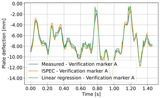
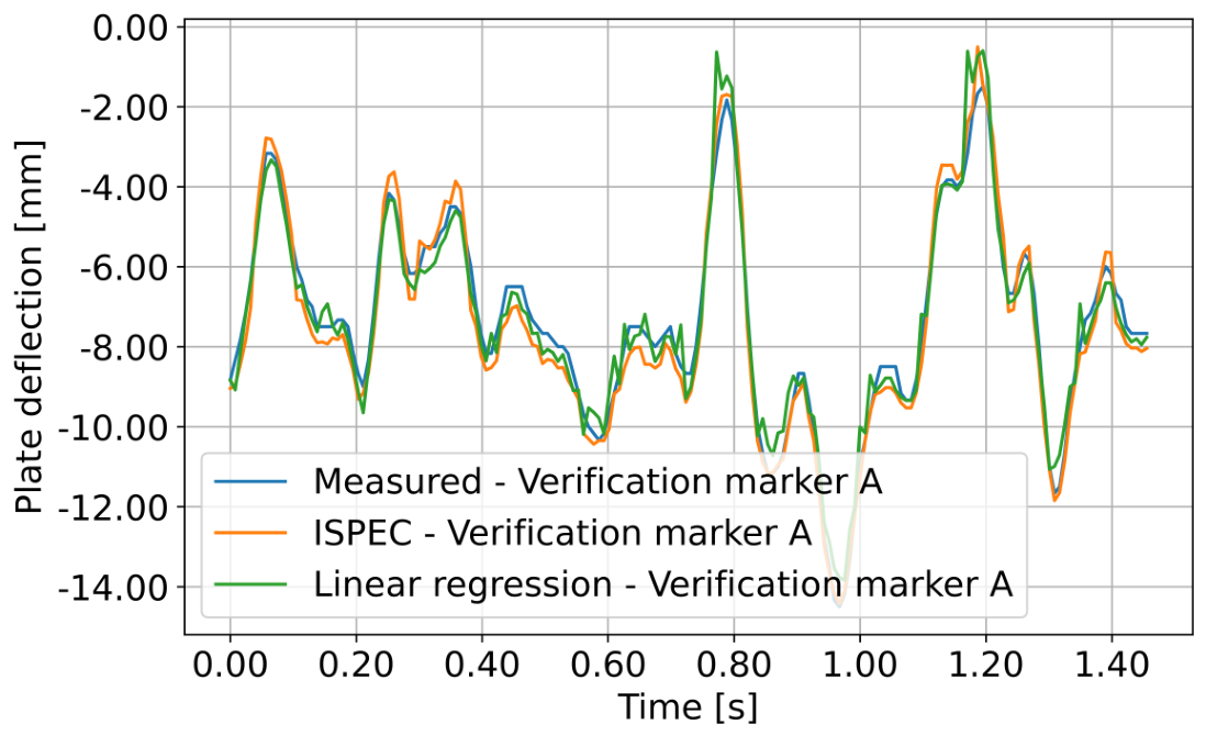
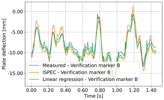
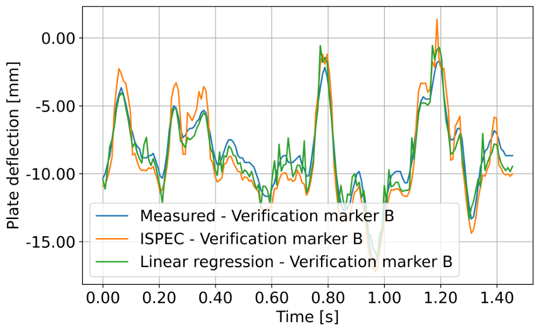
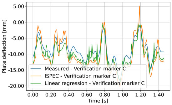
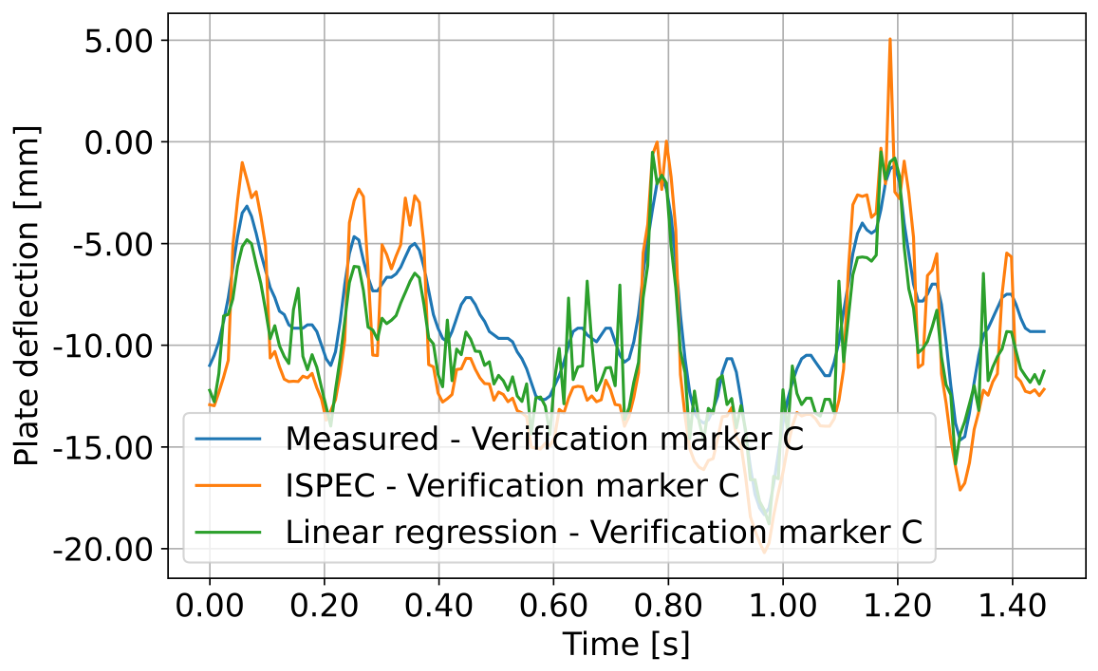
Figure 10, Figure 11 and Figure 12 show the measured deflection histories together with the corresponding reconstructions obtained using both the proposed regression-based approach and ISPEC. In all cases, both methodologies reproduce the main temporal evolution of the measured response, including the dominant deflection peaks, the principal oscillation phases, and the overall amplitude range. This demonstrates that the modal bases predicted from the seven input markers contain sufficient information to estimate the plate deflection at locations that are not directly involved in the modal inversion.

Figure 10. Measured and reconstructed deflection at verification marker A.

Figure 11. Measured and reconstructed deflection at verification marker B.

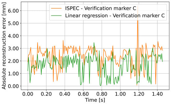
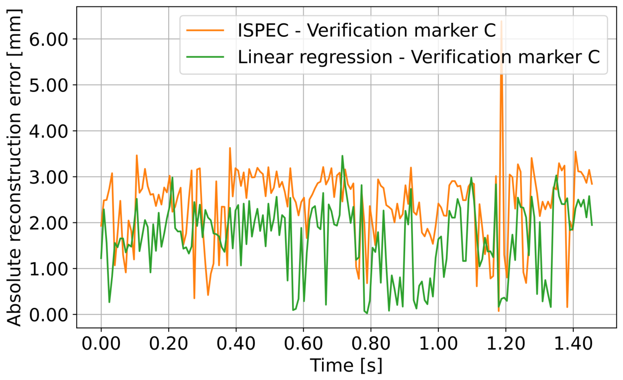
Figure 12. Measured and reconstructed deflection at verification marker C.

At marker A, both reconstruction strategies show good agreement with the measured signal throughout most of the analysed time window. The main peaks and valleys are accurately reproduced, with only minor local discrepancies. At markers B and C, the differences between the two approaches become more evident. The reconstruction obtained using the proposed regression-based modal selection (green curve) follows the measured response (blue curve) more closely than the ISPEC-based reconstruction (orange curve), which tends to overestimate the displacement peaks and, consequently, the oscillation amplitude. This behaviour is particularly evident at marker C, which represents the most demanding validation point because it is located farthest from the measurement region and closest to the fluid excitation. In this case, the regression-based approach provides a noticeably better agreement with the experimental signal, demonstrating its improved capability to reconstruct the structural response in regions where the deformation is more strongly influenced by the external loading.

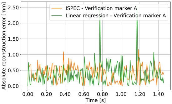
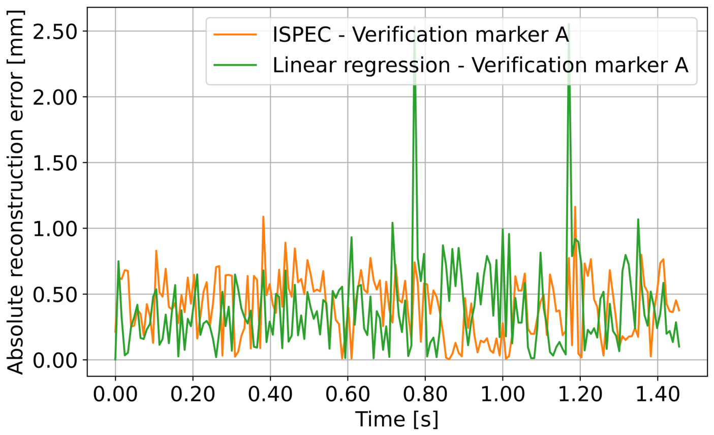
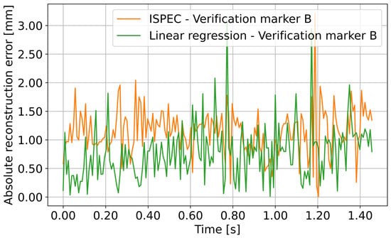
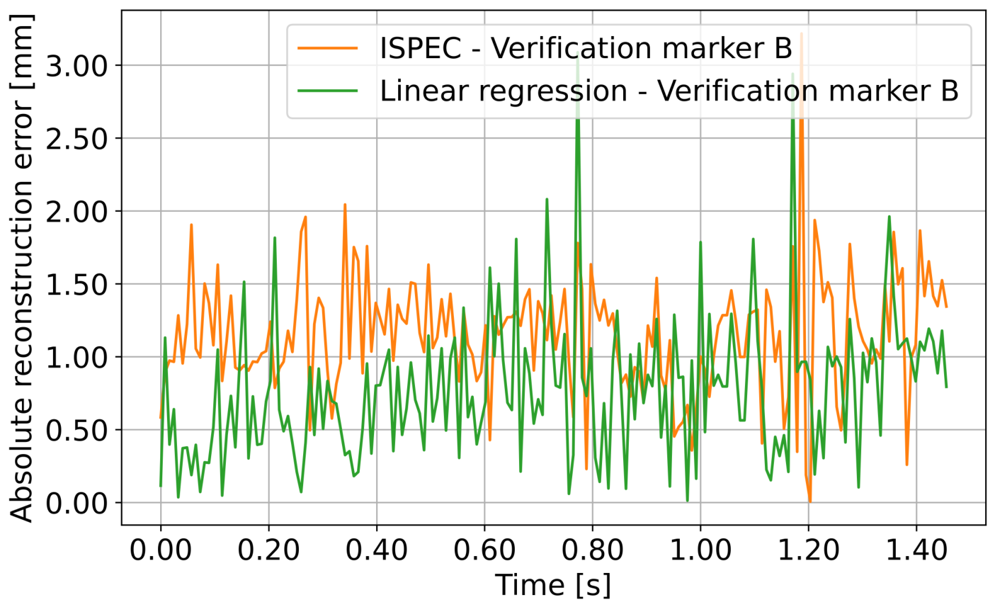
The absolute reconstruction errors obtained with the proposed regression-based approach and the ISPEC-based methodology are compared in Figure 13, Figure 14 and Figure 15. At marker A, both approaches provide a comparable level of accuracy, with sub-millimetric errors over most of the analysed time window. The ISPEC-based reconstruction exhibits slightly lower error peaks, resulting in a marginally smaller RMSE. However, moving towards markers B and C, the advantages of the proposed methodology become increasingly evident. The regression-based approach consistently produces smaller reconstruction errors, whereas the ISPEC-based reconstruction tends to amplify the displacement peaks, leading to larger instantaneous errors. This behaviour is particularly pronounced at marker C, which is located closest to the fluid excitation and farthest from the measurement region, where the reconstruction problem is most demanding.

Figure 13. Absolute reconstruction error at verification marker A.

Figure 14. Absolute reconstruction error at verification marker B.

Figure 15. Absolute reconstruction error at verification marker C.

The quantitative comparison is reported in Table 2, Table 3 and Table 4.

Table 2. Comparison between the proposed regression-based modal selection and the ISPEC-based approach. The best value for each verification marker is highlighted in bold.

Marker	Method	RMSE [mm]	NRMSE [%]
A	Lin. Regression	0.514	3.956
	ISPEC	0.468	3.596
B	Lin. Regression	0.906	6.040
	ISPEC	1.217	8.112
C	Lin. Regression	1.820	10.603
	ISPEC	2.530	14.740

Table 3. Absolute reconstruction error statistics. The best value for each verification marker is highlighted in bold.

Marker	Method	Mean [mm]	Max [mm]
A	Lin. Regression	0.386	2.553
	ISPEC	0.403	1.163
B	Lin. Regression	0.771	3.088
	ISPEC	1.149	3.217
C	Lin. Regression	1.645	3.454
	ISPEC	2.398	6.386

Table 4. Comparison of the maximum normalised cross-correlation and the corresponding time lag between the measured and reconstructed deflection signals. A zero lag indicates that both reconstruction methods preserve the temporal evolution of the measured response without introducing phase shifts. The best value for each verification marker is highlighted in bold.

Marker	Method	Maximum Cross-Correlation	Lag [Samples]	Lag [s]
A	Lin. Regression	0.979	0	0.000
	ISPEC	0.990	0	0.000
B	Lin. Regression	0.955	0	0.000
	ISPEC	0.971	0	0.000
C	Lin. Regression	0.924	0	0.000
	ISPEC	0.945	0	0.000

At verification marker A, located closest to the measurement region, both methodologies provide comparable reconstruction accuracy. In this case, the ISPEC-based approach achieves slightly lower RMSE and NRMSE values, indicating that both modal selection strategies are equally effective when the reconstruction is performed close to the input measurements.

A different behaviour is observed at markers B and C, where the proposed regression-based modal selection consistently outperforms ISPEC. At marker B, the RMSE decreases from $1.217\mathrm{mm}$ to $0.906\mathrm{mm}$, while the NRMSE decreases from $8.11\%$ to $6.04\%$. The improvement becomes even more significant at marker C, where the RMSE decreases from $2.530\mathrm{mm}$ to $1.820\mathrm{mm}$, and the NRMSE is reduced from $14.74\%$ to $10.60\%$. The statistics of the absolute error also show a consistent reduction in the mean and maximum errors, confirming that the proposed regression-based criterion provides a more accurate reconstruction not only on average but also during the largest deformation events.

The maximum normalised cross-correlation remains very high for both methodologies, ranging from 0.924 to 0.990, with zero temporal lag in all verification cases. This indicates that both approaches correctly reconstruct the temporal evolution of the structural response and preserve the phase of the measured signal. The improvement introduced by the proposed methodology therefore does not arise from a better temporal alignment, but from a more accurate estimation of the deformation amplitude. This behaviour is consistent with the proposed regression-based modal selection criterion, which explicitly optimises the agreement between reconstructed and reference displacement fields through the regression slope and intercept, thereby reducing the amplitude overestimation observed for the ISPEC-based reconstruction.

4.4. Computational Performance

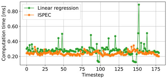
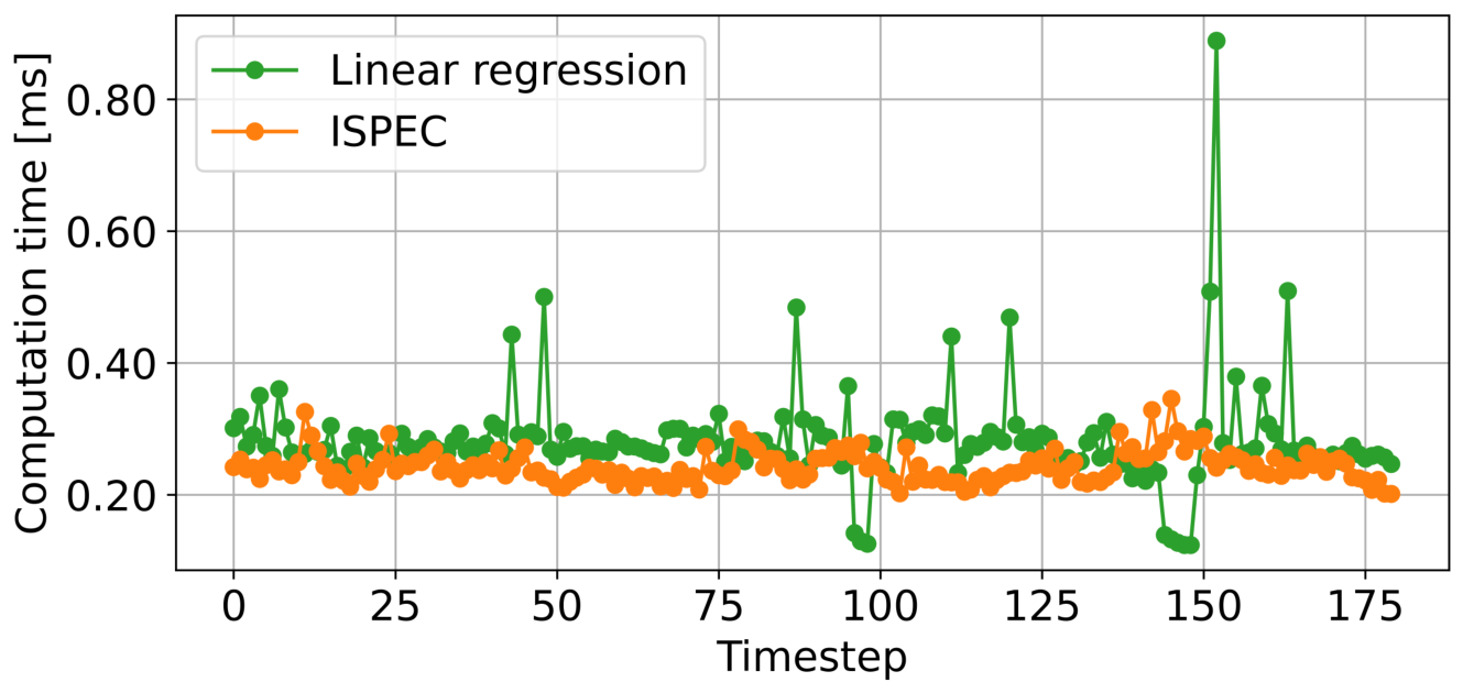
The computational performance of both reconstruction strategies was evaluated over the analysed monitoring window. The measured computation time includes the prediction of the active modal subset by the Random Forest classifier, the computation of the modal coordinates, and the reconstruction of the full-field deflection through modal superposition. The resulting computation times are reported in Figure 16.

Figure 16. Computation time per timestep for the proposed regression-based approach and the ISPEC-based methodology.

The proposed regression-based methodology requires an average computation time of $0.280\mathrm{ms}$, with a maximum value of $0.889\mathrm{ms}$, whereas the ISPEC-based approach requires $0.242\mathrm{ms}$ on average and reaches a maximum of only $0.345\mathrm{ms}$. Considering the image acquisition frequency of $123\mathrm{fps}$, the available processing time between two consecutive frames is approximately $8.13\mathrm{ms}$. Consequently, the average computation time corresponds to approximately $3.4\%$ of the available frame interval for the proposed methodology and $3.0\%$ for the ISPEC-based approach. Even the maximum computation time of the proposed method represents only about $11\%$ of the available acquisition interval, remaining well below the real-time constraint.

The slightly higher computational cost of the regression-based methodology is mainly associated with the larger variety of modal subsets predicted during the monitoring process, which leads to a greater number of pseudo-inverse evaluations during the reconstruction stage. Nevertheless, the difference with respect to the ISPEC-based approach is negligible from a practical standpoint, since both methods complete the modal identification and reconstruction well within the available acquisition time. These results demonstrate that the proposed regression-based modal selection improves reconstruction accuracy while fully preserving the real-time capability of the monitoring framework.

5. Conclusions

A machine learning-guided framework for real-time modal reconstruction of flexible structures from sparse vision-based displacement measurements has been presented. The main contribution is a regression-based modal selection criterion that identifies the modal subset according to its capability to reproduce the reference displacement field. Unlike ISPEC, which selects modes according to their energetic contribution, the proposed criterion directly targets reconstruction accuracy and is combined with a Random Forest classifier for real-time modal subset prediction.

Experimental validation on a flexible aluminium plate subjected to unsteady water-flow excitation demonstrated the effectiveness of the approach. Using seven optical measurement points, the structural response was reconstructed at independent verification locations closer to the fluid excitation. At the most demanding verification marker, the proposed approach reduced the NRMSE from $14.74\%$ with ISPEC to $10.60\%$, corresponding to an improvement of $28.07\%$. Both methods preserved the temporal evolution of the measured response, with high cross-correlation and zero temporal lag, while the regression-based approach provided a more accurate reconstruction of the displacement amplitudes. The different modal subsets and relative modal contributions identified by the two classifiers further confirm the advantage of selecting the modal basis according to reconstruction capability.

The proposed framework also satisfies the requirements for real-time implementation. The average and maximum computation times were $0.280\mathrm{ms}$ and $0.889\mathrm{ms}$, respectively, both well below the $8.13\mathrm{ms}$ interval between consecutive frames at $123\mathrm{fps}$.

The present results are limited to the investigated plate geometry, water-flow excitation, and measurement configuration. The FE model provides the spatial modal basis and training deformation states without explicitly reproducing the complete fluid–structure interaction, including hydrodynamic added-mass and damping effects. Moreover, the number and distribution of the measurement locations can influence the modal reconstruction. The current formulation also treats each acquired frame as an independent instantaneous deformation state. Consequently, it does not aim to reconstruct unresolved temporal dynamics beyond the acquisition bandwidth, although FE mode shapes associated with higher natural frequencies can still be employed as spatial basis functions.

Future work will assess repeatability and generalisation under different loading conditions, geometries, and measurement configurations, as well as extend the framework to multi-component displacement reconstruction. The introduction of temporal relationships between consecutive deformation states will also be investigated. In such a dynamic formulation, the acquisition bandwidth and possible aliasing effects would become explicit constraints of the reconstruction procedure.

References

- An accurate modal method for computing response to periodic excitation. Comput. Struct. 1997, 63, 625–631. [CrossRef] [Scilit]
- Strzalka, C.; Marinkovic, D.; Zehn, M.W. Stress mode superposition for a priori detection of highly stressed areas: Mode normalisation and loading influence. J. Appl. Comput. Mech. 2021, 7, 1698–1709. [Google Scholar] [CrossRef] [Scilit]
- Nieto, M.; Elsayed, M.; Walch, D. Modal participation factors and their potential applications in aerospace: A Review. In Proceedings of the Canadian Society for Mechanical Engineering International Congress 2018, Toronto, ON, Canada, 27–30 May 2018. [Google Scholar]
- Schwarz, B.J.; Richardson, M.H. Linear superposition and modal participation. In Proceedings of the Topics in Modal Analysis I, Volume 7: Proceedings of the 32nd IMAC, A Conference and Exposition on Structural Dynamics, 2014; Springer: Berlin/Heidelberg, Germany, 2014; pp. 161–172. [Google Scholar] [CrossRef] [Scilit]
- Kant, T.; Arora, C.; Varaiya, J. Finite element transient analysis of composite and sandwich plates based on a refined theory and a mode superposition method. Compos. Struct. 1992, 22, 109–120. [Google Scholar] [CrossRef] [Scilit]
- Wang, M.; Sheng, X. Combining empirical wavelet transform and transfer matrix or modal superposition to reconstruct responses of structures subject to typical excitations. Mech. Syst. Signal Process. 2022, 163, 108162. [Google Scholar] [CrossRef] [Scilit]
- Semblat, J.F.; Duval, A.M.; Dangla, P. Modal superposition method for the analysis of seismic-wave amplification. Bull. Seismol. Soc. Am. 2003, 93, 1144–1153. [Google Scholar] [CrossRef] [Scilit]
- Fulici, M.; Belardi, V.; Dalla Palma, M.; Liuzzo, G.; Paoletti, D.; Vivio, F.; Fanelli, P. Effects of seismic isolation on the dynamic behaviour of the DTT torus complex during earthquake events. Fusion Eng. Des. 2024, 203, 114476. [Google Scholar] [CrossRef] [Scilit]
- Gao, Z.; Zhao, M.; Du, X.; Wang, J. Effective-mode superposition response spectrum method for three dimensional seismic response analysis of underground structures. Soil Dyn. Earthq. Eng. 2023, 174, 108161. [Google Scholar] [CrossRef] [Scilit]
- Foss, G.; Haugse, E. Using modal test results to develop strain to displacement transformations. In Proceedings of the 13th International Modal Analysis Conference, Nashville, TN, USA, 13–16 February 1995; Volume 2460, p. 112. [Google Scholar]
- Pisoni, A.C.; Santolini, C.; Hauf, D.E.; Dubowsky, S. Displacements in a vibrating body by strain gage measurements. In Proceedings—SPIE the International Society for Optical Engineering; Citeseer: Princeton, NJ, USA, 1995; p. 119. [Google Scholar]
- Li, L.; Zhong, B.S.; Geng, Z.Y.; Sun, W. Structural Shape Reconstruction of FBG Flexible Plate Using Modal Superposition Method. In Proceedings of the International Design Engineering Technical Conferences and Computers and Information in Engineering Conference, Cleveland, OH, USA, 6–9 August 2017; Volume 58226, p. V008T12A038. [Google Scholar] [CrossRef] [Scilit]
- Cheng, Y.; Li, Z.; Wang, G.; Peng, C.; Zhang, L.; Yang, W.; Jiang, M.; Sui, Q. Strain field reconstruction of crossbeam structure based on load–strain linear superposition method. Smart Mater. Struct. 2021, 30, 075020. [Google Scholar] [CrossRef] [Scilit]
- Liuzzo, G.; Fanelli, P. Modal Reconstruction Algorithm for Structural Health Monitoring for Evaluating Time-Variant Machine Deformations. Eng. Proc. 2026, 131, 4. [Google Scholar] [CrossRef] [Scilit]
- Liuzzo, G.; Fanelli, P. Non-Destructive Structural Deformation Reconstruction via Data-Driven Modal Superposition. Appl. Sci. 2026, 16, 2168. [Google Scholar] [CrossRef] [Scilit]
- Yan, J.; Cheng, Y.; Zhang, L.; Li, Z.; Xu, T.; Zhang, F.; Jiang, M.; Sui, Q. Displacement field reconstruction technique for plate-like structures based on model superposition method. Meas. Control. 2023, 56, 654–667. [Google Scholar] [CrossRef] [Scilit]
- Li, S.; Wang, S.; Cheng, Y.; Peng, C.; Wu, X.; Zhao, J.; Jiang, M.; Zhang, L. Strain/displacement field reconstruction and load identification of bracket arm structure of high-speed maglev train based on superposition conversion algorithm. Measurement 2024, 224, 113945. [Google Scholar] [CrossRef] [Scilit]
- Li, Z.; Cheng, Y.; Zhang, L.; Wang, G.; Ju, Z.; Geng, X.; Jiang, M. Strain field reconstruction of high-speed train crossbeam based on FBG sensing network and load-strain linear superposition algorithm. IEEE Sens. J. 2021, 22, 3228–3235. [Google Scholar] [CrossRef] [Scilit]
- Choi, S.M.; Kim, M.H. Shape reconstruction from partially missing data in modal space. Comput. Graph. 2002, 26, 701–708. [Google Scholar] [CrossRef] [Scilit]
- Yang, J.; Fu, Z.; Zou, Y.; He, X.; Wei, X.; Wang, T. A response reconstruction method based on empirical mode decomposition and modal synthesis method. Mech. Syst. Signal Process. 2023, 184, 109716. [Google Scholar] [CrossRef] [Scilit]
- Kang, L.H.; Kim, D.K.; Han, J.H. Estimation of dynamic structural displacements using fiber Bragg grating strain sensors. J. Sound Vib. 2007, 305, 534–542. [Google Scholar] [CrossRef] [Scilit]
- Zhu, Y.; Wang, Y.; Qiao, B.; Fu, S.; Liu, M.; Luo, X.; Chen, X. Full-field dynamic strain reconstruction of rotor blades under multi-mode vibration. Measurement 2022, 201, 111670. [Google Scholar] [CrossRef] [Scilit]
- Cheng, Y.; Zhang, L.; Jiang, M.; Sui, Q. Strain/displacement field reconstruction and load identification of high-speed train load-bearing structure based on linear superposition method. IEEE Trans. Instrum. Meas. 2022, 71, 1–8. [Google Scholar] [CrossRef] [Scilit]
- Li, M.; Jia, D.; Wu, Z.; Qiu, S.; He, W. Structural damage identification using strain mode differences by the iFEM based on the convolutional neural network (CNN). Mech. Syst. Signal Process. 2022, 165, 108289. [Google Scholar] [CrossRef] [Scilit]
- Yan, J.; Zhang, M.; Sun, L.; Xie, Z.; Zhao, Z.; Zhang, J.; Wang, F. Shape sensing of a wind turbine tower based on a one-sided four-node quadrilateral inverse shell element with a coupling functional. Thin-Walled Struct. 2025, 215, 113577. [Google Scholar] [CrossRef] [Scilit]
- Horas, C.S.; De Jesus, A.M.; Ribeiro, D.; Calçada, R. Efficient multiscale methodology for local stress analysis of metallic railway bridges based on modal superposition principles. Eng. Fail. Anal. 2022, 138, 106391. [Google Scholar] [CrossRef] [Scilit]
- Cui, J.; Zeng, J.; Shao, F.; Wang, S.; Liu, S.; Huang, Y.; Tang, S. Reconstruction of composite panel deformation based on modal superposition and calibration method by fiber optic sensors. In Proceedings of the First Conference on Distributed Optical Fiber Sensing Technology and Applications (DOFS 2024); SPIE: Bellingham, WA, USA, 2025; Volume 13654, pp. 327–339. [Google Scholar] [CrossRef] [Scilit]
- Liuzzo, G.; Parisi, M.; Fanelli, P. Analytical Formulation of New Mode Selection Criteria in the Reconstruction of Static Deformation of Structures Through Modal Superposition. Appl. Mech. 2025, 6, 67. [Google Scholar] [CrossRef] [Scilit]
- Bogert, P.; Haugse, E.; Gehrki, R. Structural shape identification from experimental strains using a modal transformation technique. In Proceedings of the 44th AIAA/ASME/ASCE/AHS/ASC Structures, Structural Dynamics, and Materials Conference, Norfolk, VA, USA, 7–10 April 2003. [Google Scholar]
- Esposito, M.; Gherlone, M. Composite wing box deformed-shape reconstruction based on measured strains: Optimization and comparison of existing approaches. Aerosp. Sci. Technol. 2020, 99, 105758. [Google Scholar] [CrossRef] [Scilit]
- Liuzzo, G.; Parisi, M.; Fanelli, P. Modal Shapes Selection Criterion for Modal Reconstruction Aimed at Structural Health Monitoring. Eng. Proc. 2025, 85, 39. [Google Scholar] [CrossRef] [Scilit]
- Liuzzo, G.; Meloni, S.; Fanelli, P. Structural Health Monitoring of a Lamina in Unsteady Water Flow Using Modal Reconstruction Algorithms. Fluids 2025, 10, 276. [Google Scholar] [CrossRef] [Scilit]
- Ansys APDL Element Reference, Release 2020 R2; Ansys Inc.: Southpointe, PA, USA, 2020.
- Hodson, T.O. Root mean square error (RMSE) or mean absolute error (MAE): When to use them or not. Geosci. Model Dev. Discuss. 2022, 2022, 1–10. [Google Scholar] [CrossRef] [Scilit]
Disclaimer/Publisher’s Note: The statements, opinions and data contained in all publications are solely those of the individual author(s) and contributor(s) and not of MDPI and/or the editor(s). MDPI and/or the editor(s) disclaim responsibility for any injury to people or property resulting from any ideas, methods, instructions or products referred to in the content. |
© 2026 by the authors. Licensee MDPI, Basel, Switzerland. This article is an open access article distributed under the terms and conditions of the Creative Commons Attribution (CC BY) license.