


Abstract
Surface normal estimation is a fundamental step in many applications, including robotics, manufacturing inspection and quality control. Reliable surface normal information is essential for accurate surface reconstruction, defect detection, and geometric analysis. In this paper, different approaches for estimating surface normal vectors from point cloud data are investigated, with particular focus on their suitability for generating ground-truth surface normals. Such ground-truth measurements are required to evaluate and validate surface normal estimation techniques used in practical metrology and 3D sensing systems in accordance with established surface texture standards such as ISO 25178. The analysis focuses on methods based on neighbourhood clustering followed by a surface normal fitting procedure. In addition, the influence of point cloud noise on the accuracy and stability of the estimated normals is systematically studied. By comparing the performance of different estimation strategies under different noise conditions, their suitability for generating reliable reference surface normals is investigated. The results demonstrate how point cloud characteristics and noise levels affect the robustness of surface normal estimation and highlight the advantages and limitations of commonly used approaches. The proposed analysis provides practical guidance for selecting appropriate methods when generating ground-truth surface normals for the validation of optical and geometric measurement systems. To show that the studied approaches can be used for surface normal estimation independent of metrology equipment, they are applied to the point clouds acquired from laser scanners, confocal optical measurement equipment, coherence scanning interferometers, and fringe projection systems with a variety of test objects. The results show that the studied approaches can estimate the surface normals. Highly accurate surface normal estimation may ease surface texture studies. The findings contribute to improving the reliability of point cloud analysis and surface normal estimation in manufacturing metrology and related applications.
1. Introduction
Precise knowledge of surface normal vectors is essential in many manufacturing and inspection processes. Applications such as robotic surface inspection, manipulation, tooling, and machining can be performed more effectively when accurate surface normal information is available [1,2,3]. Surface normals are fundamental descriptors of local surface geometry and are widely used in tasks such as surface reconstruction, defect detection, and geometric analysis. In the absence of a Computer-Aided Design (CAD) model of the workpiece, the object surface normals need to be measured using appropriate optical metrology equipment and performing the required estimation procedure. Optical and geometric metrology systems are commonly employed to acquire surface data in the form of point clouds. For example, a laser tracker equipped with a suitable scanning device can provide accurate point cloud measurements of complex surfaces. Surface normal estimation algorithms can then be applied directly to the acquired point cloud to determine the local surface orientation. However, the reliability of these estimated normals depends strongly on the estimation method and the characteristics of the measured data. Consequently, robust approaches for evaluating the accuracy of estimated surface normals are required. Reflectance transformation imaging (RTI) approaches, which capture high-quality images of an object surface under various illumination conditions [4] constitute another class of surface normal estimation techniques. RTI methods were originally designed for visualisation of surface texture on cultural heritage objects such as archaeological artefacts and ancient graffiti [5]. Accurate RTI measurements require carefully designed hardware configurations, appropriate image processing algorithms, and reliable surface normal estimation procedures. In cases where analytical surface normal values are unavailable, surface normals estimated from high-precision point cloud measurements can be used as reference data for assessing the accuracy of RTI-based techniques.
Several approaches have been proposed to estimate surface normal vectors of an object surface from point cloud data. Typically, these approaches involve two main steps. In the first step, one of the clustering approaches, either K-nearest neighbours or radially bounded nearest neighbour (RBNN), is used to cluster points around each point within the point cloud [6,7]. Then a surface normal estimation approach is applied to the points within each cluster to generate the corresponding surface normal values. The existing approaches are categorised as indirect and direct. In indirect approaches, a 3D plane is fitted to the points within each cluster. A cost function is defined as the deviation of the points in each cluster from the estimated plane. The optimal surface would have the least deviation from the given points. The surface normal vector can then be extracted by separating the surface normal vector and the corresponding bias term within the plane. The direct geometrical approaches include taking the weighted geometric mean of the vectors connecting all points in the cluster over the measurement area.
The clustering algorithm and surface normal estimation technique influence the estimation accuracy. Two main approaches are identified by this article within the literature to evaluate the estimation accuracy of the estimated surface normal. The first category evaluates the detected surface normal against the original point cloud by testing the orthogonality of the detected surface normal against the set of points within the cluster. The second approach evaluates the estimated surface normals against the available ‘ground truth’.
In this paper, both categories of surface normal detection, indirect techniques and direct approaches, are studied. Several test objects, including regular 3D geometrical shapes with precisely known surface normals and digital objects scanned by laser scanners, are used within the experimental validations. A comprehensive accuracy comparison is performed between the surface normal detection techniques using the 3D regular geometrical shapes. Subsequently, the influence of clustering parameters, including cluster size, is analysed under varying noise conditions using digitally scanned objects. Based on the results obtained, the surface normals for a medallion object are estimated using point cloud data acquired by a laser scanning system. The RBNN clustering approach, combined with a least squares surface-fitting method, is applied for the final estimation. To demonstrate the applicability of the studied approaches for metrology, several types of metrology equipment are chosen: laser scanners, confocal optical measurement equipment, coherence scanning interferometers, and fringe projection systems. Using this metrology equipment, high-resolution point clouds of 3D objects are acquired. The 3D objects used for this study include heritage objects, numismatics, and 3D-printed objects. Surface normal estimation techniques applied to these point clouds are shown to be successful in estimating surface normals. It is further shown that using the estimated surface normals, the surface texture of the studied objects is easily recognisable. Finally, practical guidelines are provided for selecting the appropriate clustering and surface normal estimation techniques for reliable surface normal generation from point cloud data. The key points of the present paper are as follows.
- Surface normal ground truth is of high importance for measurement and validation purposes. Several surface normal estimation techniques using point cloud data are evaluated, and their performance and suitability for estimating ground-truth surface normal vectors are assessed. The particular focus is on their suitability for generating ground-truth surface normals from a high-resolution and dense point cloud.
- The surface normal estimation algorithms investigated in this paper include KNN and RBNN clustering algorithms as their first step. However, these clustering algorithms require design parameters, including the K value in KNN and the radius value in RBNN. Some guidelines are provided to select these design parameters, which may accelerate the process of ground-truth surface normal estimation.
- Multiple metrology equipment including laser scanners, confocal optical measurement equipment, coherence scanning interferometers, and fringe projection systems are used to acquire point clouds from 3D objects including cultural heritage objects, 3D-printed objects, and coins. The applicability of the investigated surface normal estimation techniques for these objects is given.
This paper is organised as follows. In Section 2, the overall proposed ground-truth surface normal generation algorithm, and surface normal estimation approaches are studied. Uncertainty analysis of surface normal measurement techniques is given in Section 3. ISO 25178 standard and associated artefacts are studied in Section 4. Results are given in Section 5, followed by Section 6, which presents the concluding remarks, and the references are given as the last section. Appendix A of the paper includes some of the variables used for uncertainty analysis purposes.
2. Overall Proposed Ground-Truth Surface Normal Generation Algorithm
To generate ground-truth surface normals in the absence of a precise 3D CAD model of the object, the surface geometry must first be captured in the form of a 3D point cloud. A point cloud represents a collection of points describing the spatial coordinates of the object surface in 3D space. Such data is typically acquired using laser scanners through dedicated data acquisition software. Prior to surface normal estimation, several preprocessing steps may be required to ensure the quality of the point cloud data. These steps may include cropping the point cloud to isolate the region of interest, aligning and rotating the dataset to a consistent coordinate system, and removing points generated as a result of the environment. These operations ensure that a clean and accurate point cloud is available for subsequent analysis. The surface normal estimation is then performed by identifying clusters of neighbouring points that belong to the same local surface region.
For each point within the point cloud, a set of neighbouring points is determined using a clustering method. A surface normal estimation technique is subsequently applied to each cluster in order to determine the local surface orientation associated with that region. The surface normals generated using this approach are obtained directly from the measured point cloud and therefore do not rely on the availability of a CAD model. Consequently, the method can be used to generate ground-truth surface normals for applications such as surface texture analysis and validation of other normal estimation techniques. Furthermore, this approach is particularly suitable for freeform metrology and reverse engineering applications, where CAD models may be unavailable due to obsolete components, manufacturing deviations, or surface wear and damage. The overall workflow of the proposed ground-truth surface normal estimation procedure is illustrated in Figure 1.
Figure 1.
Surface normal estimation flowchart.
Consider a set of n points , which shall be represented by an data matrix
where represents the 3D coordinate of the measured point. The corresponding surface normal for every point in the point set, , is represented as . To calculate this surface normal, it is required to define a set of points in the neighbourhood of represented by and its augmented neighbourhood which includes represented by . The neighbourhood techniques to define , and are explained in this section.
2.1. Neighbourhood Assignment Through Clustering
The crucial step to find the normal vector associated with a point is to select an appropriate neighbourhood for the corresponding point. Too large a set of points results in too smooth a set of surface normal vectors, which does not sufficiently represent the details of the surface. On the other hand, if the neighbour set is selected too small, it may result in a noisy and inaccurate estimation of the normal vectors. Within the simulation section of this paper, the effect of cluster size on the surface normal evaluation will be studied.
In the literature, there exist several neighbouring point selection algorithms from which K-nearest neighbour (KNN) and radially bounded nearest neighbour graph (RBNN) are investigated.
2.1.1. K-Nearest Neighbour (KNN)
Within the K-nearest neighbours algorithm, each point is connected with its K-nearest neighbouring points (see Figure 2a). The distance can be calculated using the Euclidean or any other metric [7,8]. In Figure 2a the vector is the surface normal for the point P and its neighbouring points.
Figure 2.
(a) K-nearest neighbours; (b) radially bounded nearest neighbour graph.
2.1.2. Radially Bounded Nearest Neighbour Graph (RBNN)
The radially bounded nearest neighbour graph is constructed upon a group of points whose distance to the given point is less than a given radius (see Figure 2b). This type of neighbour assignment can be defined in a mathematical form as follows [6,7].
where the point is a point from the point cloud for which its neighbourhood is constructed, is the distance function between and points, is a positive value, are the points which lie within radius around point , and is the associated neighbourhood set of points within the point cloud. The distance function considered in this paper is Euclidean.
2.2. Calculating Surface Normal from a Set of Points
2.2.1. Optimisation-Based Surface Normal Detection Techniques
a. PlaneSVD is a classical approach to fit the surface normal associated with a number of points given within the point set, which includes ’s, and . The equation of the corresponding planar surface is given as [9,10]. The vector components represent the surface normal vector associated with the surface .
Therefore, it is required to solve the following minimisation problem:
where 1m = [1 1 … 1]T represents an vector of ones and includes the surface normal vector () and a bias term () corresponding to the plane fitted to the points within. The matrix is defined as follows.
To solve this minimisation problem, the following SVD problem is solved [11].
The is the vector in the matrix corresponding to the smallest singular value in .
b. The problem of fitting the surface which includes all the points in a given cluster can be solved using a least squares approach. It is known that for points on the planar surface, the following equality holds [12].
Therefore, the problem can be reformulated as a regressor-parameter type of equation.
where and are the x, y, and z components of , and and are the surface parameters, and the following equations hold.
The solution to the least squares problem in (6) is calculated using a pseudo-inverse operator as follows.
If all ’s are the same, the matrix would be rank deficient. To solve this problem, it is suggested to keep values in ’s , and ’s , in the matrix and push values in ’s to the matrix. Otherwise, the matrix would be rank deficient and its inverse matrix would not exist.
c. Since for the points located on the plane constructed upon the given points, the following condition holds: , another possible solution to the surface normal estimation problem can be found by minimising the cost function
subject to:
The solution to this optimisation problem is equivalent to finding the eigenvector corresponding to the minimum eigenvalue of the following matrix.
Therefore, the matrix corresponding to each is a matrix. The eigenvector solution to the problem will provide an approximation of the plane and, consequently, the surface normal vector associated with the points.
d. PlanePCA is another surface normal estimation technique. This algorithm involves removing the common component among the given point set to make the bias term of the plane equal to zero. Therefore, the algorithm reduces the total number of parameters used during the minimisation procedure to three [13,14].
where , and
The solution to the minimisation problem in (12) is obtained as the singular vector of associated with the smallest singular value. This approach is called PlanePCA, as the solution is obtained by performing principal component analysis on and finding the principal component with the smallest variance (the first PCA component).
e. Vector SVD is an alternative technique in which the surface normal is calculated to minimise the cosine of the angle between the tangential vectors from to and the normal vector by minimising the following cost function [15].
f. To improve the robustness of the surface normal estimation, an equivalent formulation to VectorSVD is considered which is centred not on the reference point () but rather around the arithmetic mean of the members of the cluster (). For each neighbourhood , a square matrix is considered as follows [14].
where is defined in (14). The eigenvector corresponding to the minimum eigenvalue of is taken as the surface normal at the point . The resulting surface normal minimises the following cost function.
g. Renormalisation approach is an iterative process of finding the optimal plane under noisy conditions. In the first step, the following two matrices are defined [16].
The process of fitting the optimal surface is iterated for a few steps using the following procedure until the parameters of the surface have converged to the optimal solution [12,16].
- I.
- Initialise for all and values, and , then compute the matrices and .
- II.
- Update the matrix using , then calculate the smallest eigenvalue and eigenvector of .
- III.
- If the smallest eigenvalue of is close to zero, i.e., , its corresponding eigenvector is the solution to the surface normal estimation problem and stop the procedure. Otherwise, continue to the next step.
- IV.
- Update the parameters , and as follows.
- V.
- Jump to step II.
Note that it is required to avoid singularity in . Therefore, a threshold value very close to zero is usually set for the denominator of to avoid singularity.
h. Another approach to decrease the effect of the points far from is by using nonlinear functions such as Gaussian functions, which provide higher gains close to and lower gain values for points far from . Then , and may be modified as
i. An undesirable property of the algorithm mentioned in (e) is that the impact of points closer to the reference point is less than the impact of points further away. This may cause some error in the calculated surface normal value. Therefore, the normalised versions of and may be more desirable. In the case of the reference position , is written as follows [14].
and in the case of the reference point of , is rewritten
2.2.2. Direct Methods for Surface Normal Estimation
This method is an alternative surface normal estimation algorithm to find the weighted average of the surface normal vector over triangles formed by pairs of neighbours within number of neighbours of [17]. This method does not involve optimisation to obtain the surface normal. The points within the neighbours for are represented by . Although there exist number of pairs to be selected to construct vectors in the neighbourhood, only pairs of points are considered. In other words, each point is considered in consecutive order with the next point within the neighbourhood. The surface normal in this case is calculated as follows.
where for a basic averaging over all triangles within the neighbourhood of and, represents the cross product [18]. However, there exist alternative selections for each resulting in different estimations. Among different possible choices for , area weighted approach is selected. In this algorithm, for each triangle is considered equal to the magnitude of its area [19,20].
Therefore, the value of is cancelled and the formula to calculate reduces to finding the average value of all unnormalized vectors within the neighbours of .
2.3. Surface Normal Evaluation Techniques
2.3.1. Cosine Performance Index
The cosine value of the angle between the estimated surface normal and the ground-truth surface normal is calculated. The absolute value of the inner product of the normalised estimated vector and ground-truth vector is considered as the estimation performance index.
where represents the dot product of and . The Cosine performance index for and is close to 1 in the case when these two vectors are aligned and is close to 0 when they are perpendicular to each other. If the surface normal vectors and are already normalised, the denominator of in (26) is equal to 1. Therefore, for a high-performance surface normal estimation, it is desired to have as close as possible to one.
2.3.2. Sinus Performance Index
Unlike the Cosine performance index, the Sinus performance index is defined as the result of the cross product between the estimated surface normal and the ground-truth surface normal .
In this case, for a high-performance estimation, it is desired that the Sinus performance index be close to 0. Similar to the Cosine performance index, the Sinus performance index is always a positive value in the interval of . If the surface normal vectors and are already normalised, the denominator of in (27) is equal to 1.
2.3.3. Element-Wise Performance Index
A useful performance index is to evaluate the mean Euclidean distance between the corresponding pairs of estimated and ground-truth surface normal vectors.
where is the minimum norm of the error between the estimated surface normal ( and the surface normal ( and (. It is to be noted that the surface associated with a surface normal and the surface associated with ( are two identical surfaces. This fact is illustrated in Figure 3. Therefore, needs to be formulated as (28) to avoid estimation error.
Figure 3.
Surface normals: and , which is a 180° rotated version of .
2.3.4. Direct Performance Index Using the Ground-Truth Point Cloud
A direct approach to evaluate the estimated value of the surface normal is to test whether the points within its neighbourhood are located on the planar surface associated with . Suitable neighbouring points may be selected using one of the clustering algorithms of KNN or RBNN. The points within the neighbourhood are then used for direct performance index measurement. Ideally, the inner product of the surface normal and the given surface vectors should be equal to zero [21].
The desired value for this performance index is 0, which implies that the estimated surface normal value is perpendicular to the ground-truth neighbouring vectors. The neighbouring points may be calculated using one of the clustering algorithms of KNN or RBNN.
3. Uncertainty Analysis of Surface Normal Measurement
Uncertainty analysis includes the identification process of the sources of uncertainty and statistical characteristics associated with each, including mean and variance values [22,23]. The uncertainty analysis of surface normal measurements using a laser tracker and 3D scanner is conducted in this section. Sources of uncertainty in surface normal estimation include neighbourhood size, uncertainty in point cloud measurements, surface curvature, surface normal estimation algorithm, and numerical conditioning. Point cloud measurements inherently suffer from uncertainty because of measurement uncertainty in the laser equipment. Surface reflectivity, triangulation geometry, systematic errors, and calibration errors are among the inherent sources of uncertainty for point cloud measurement using a laser tracker [23,24,25]. The curvature depends on the shape of the component; it may influence the point cloud measurement uncertainty, as too deep a valley or too high a hill may cause beam divergence and affect the angle of beam incidence for the laser measurement instrument. This may cause larger uncertainty in the point cloud and consequently larger uncertainty in surface normal measurements. Neighbourhood size is another source of uncertainty; however, this source of uncertainty is investigated in this paper using a numerical analysis in Section 5. The choice of surface normal estimation algorithm, and numerical conditions associated with them, is another source of uncertainty. The comparisons made in Section 5 demonstrate how these factors can affect the uncertainty in surface normal calculations. In this section, the uncertainty analysis of the LS algorithm due to uncertainty in point cloud measurements from the laser instrument is given. The uncertainty analysis given in this section provides the contribution of the uncertainty within the point cloud to the surface normal estimation.
Using the LS algorithm to estimate the three components of the surface normal vector results in the following equation:
where , , , , , and are as given in Appendix A. Therefore, the Gaussian error-propagation equation for the first component of the surface normal measurements () due to measurement uncertainty in the point cloud generated by the laser tracker and AS1 scanner is as follows [26].
where
The assumption made in these equations is that the parameters , and in the point cloud follow a Gaussian probability density function, and they are independent of each other [26]. Similarly, the Gaussian error-propagation equation for ’s is as follows.
where
and finally, the uncertainty in ’s is formulated as follows.
where
Therefore, having the measurement uncertainties in the point cloud measurements , , and , the measurement uncertainty in the surface normal measurements can be calculated using (31)–(33). The point cloud measurement uncertainties, including , , and are given in the laser tracker datasheet with a value less than .
4. ISO 25178 Standard and Artefacts
ISO 25178 standard defines a set of areal surface texture parameters used to quantitatively describe surface topography. These parameters are grouped into several categories, including height, spatial, hybrid, functional and feature parameters. Height parameters describe the vertical characteristics of the surface within the defined measurement area. Typical examples include arithmetical mean height , the root mean square height , the maximum peak height value , maximum pit depth value . Root mean square gradient, , is an example of a hybrid parameter that combines amplitude and spatial information. The definition of surface parameters within the ISO 25178 standard and its widespread usage among processes, companies, and nations provides a basis for mutual understanding of surface metrology.
The basic characteristics involved in ISO 25178 [27] can be tested on any of the universal calibration artefacts [28]. The calibrated artefacts allow the performance of optical measurement systems to be evaluated in terms of noise level, spatial resolution, and feature detection capability. These artefacts can be manufactured using various methods, including Two-Photon laser lithography [29], selective laser sintering [30], and selective laser melting and electron beam melting [31,32]. Surface types, including AFL, ARS, ASG, ACG, AIR, and CIN, are within the ISO 25178 standard.
Type AFL is a flat surface to evaluate optical instruments with sub-nanometric noise amplitude. Type CIN surface is a 3D chirp signal whose frequency sweeps a range of sinusoidal waves with different frequency values. This type of signal can be used to characterise the lateral resolution limitation for surface topography measurement equipment. Type ARS surface has a radial sinusoidal shape [28]. These three surface types are investigated in this paper, and the surface normal vectors associated with them are estimated under noisy conditions.
5. Results
Three experimental scenarios are considered to evaluate the performance of the surface normal estimation algorithms introduced in the previous sections. In the first scenario, geometries with known mathematical formulations are generated within the MATLAB R2025a environment to provide reference surfaces with known surface normals. In the second scenario, three standardised surface artefacts defined in the ISO 25178 framework (AFL, CIN, and ARS) are investigated. Thirdly, the point cloud obtained from various cultural heritage artefacts, numismatics, and 3D manufactured parts is evaluated. This is to provide evidence of the applicability of the studied approaches to point clouds gathered from different metrology equipment, including laser scanners, confocal optical measurement equipment, coherence scanning interferometers, and fringe projection systems. The results corresponding to these three cases are presented in Section 5.1, Section 5.2, Section 5.3, Section 5.4 and Section 5.5. To compare the robustness of the studied approaches to noisy conditions, Gaussian noise with different covariance levels is added to the point cloud associated with artefacts.
5.1. Surface Normal Estimation for Analytical Geometries
Three geometrical shapes with known mathematical formulations are considered: a semi-cylinder, semi-sphere and a pyramid. These 3D shapes are generated within the MATLAB environment to provide point clouds with known surface normals (see Figure 4). The semi-cylinder has a radius of 5 mm and a length of 5 mm, while the spherical surface has a radius of 4 mm centred at the origin. For the pyramid geometry, a square base of 7.07 mm with an apex height of 5 mm is used. The point clouds are sampled on regular grids with a spacing of 25 µm, resulting in approximately 80,000 points for each geometry. Figure 5, Figure 6 and Figure 7 present the performance of the investigated surface normal estimation algorithms when the KNN clustering method is used. The neighbourhood size k (number of elements in each cluster) varies between 4 and 10 on the horizontal axis in Figure 5, Figure 6 and Figure 7 in order to evaluate the influence of cluster size on estimation accuracy.
Figure 4.
Simulated point clouds generated in the MATLAB environment: (a) cylindrical; (b) spherical; (c) pyramid.
Figure 5.
KNN clustering algorithm for surface normal estimation of cylindrical geometry: (a) Cosine performance index; (b) element-wise performance index.
Figure 6.
KNN clustering algorithm for surface normal estimation of spherical geometry: (a) Cosine performance index; (b) element-wise performance index.
Figure 7.
KNN clustering algorithm for surface normal estimation of pyramid geometry: (a) Cosine performance index; (b) element-wise performance index.
For all geometries, the Cosine performance index remains close to unity, indicating strong agreement between the estimated and reference surface normals. The spherical geometry exhibits the highest accuracy due to its smooth curvature and absence of sharp edges. In contrast, the pyramid geometry shows slightly reduced performance, particularly near edges where abrupt changes in surface orientation occur.
Increasing the neighbourhood size generally improves estimation performance, as the inclusion of additional neighbouring points reduces the effect of local noise. The best performance is typically obtained for k = 7, representing a balance between noise suppression and preservation of local surface features.
Figure 8, Figure 9 and Figure 10 show the corresponding results when the RBNN clustering approach is used. In this case, the neighbourhood radius varies between 140 µm and 200 µm and forms the horizontal axis of Figure 8, Figure 9 and Figure 10. Similar trends are observed: increasing the neighbourhood radius generally improved estimation accuracy due to the larger number of points included in the local fitting process. However, for the pyramid geometry, large neighbourhood radii result in reduced performance near edges, where neighbouring points belonging to different surface facets were included in the estimation.
Figure 8.
RBNN clustering algorithm for surface normal estimation of cylindrical geometry: (a) Cosine performance index; (b) element-wise performance index.
Figure 9.
RBNN clustering algorithm for surface normal estimation of spherical geometry: (a) Cosine performance index; (b) element-wise performance index.
Figure 10.
RBNN clustering algorithm for surface normal estimation of pyramid geometry: (a) Cosine performance index; (b) element-wise performance index.
Among the tested Methods, the least squares (LS) approach and methods 2.2.1.f and 2.2.1.h consistently produced the most accurate results. In contrast, Method 2.2.1.c and the PlanePCA approach exhibit comparatively lower performance for several test cases.
5.2. Surface Normals for ISO 25178 Artefacts
The performance of the investigated algorithms is further evaluated using three ISO 25178 calibration artefacts: AFL (flat surface), CIN (chirp surface), and ARS (radial sinusoidal surface).
5.2.1. AFL Flat Surface
The size of the AFL flat surface is considered equal to 0.1mm, and the points are selected using grids of 1 µm intervals. To study the performance of the surface normal estimation algorithms, a noise analysis is performed. For this purpose, additive noise with normal probability distribution functions with standard deviations equal to 0.5 µm, 1 µm, 1.5 µm, 2 µm, 2.5 µm, and 3 µm is added to the point cloud in the z-dimension. Figure 11, Figure 12, Figure 13, Figure 14, Figure 15 and Figure 16 illustrate the performance of the investigated algorithms on the AFL surface when its point cloud is corrupted by noise, and KNN is used for the clustering approach. Figure 11, Figure 12, Figure 13, Figure 14, Figure 15 and Figure 16 reveal that by increasing the standard deviation of noise, the performance of surface normal estimation methods decreases. The k value within the clusters varies from 4 to 10 and is displayed on the x-axis in Figure 11, Figure 12, Figure 13, Figure 14, Figure 15 and Figure 16. The performance index generally improves as k increases because of statistical properties of the clustering approach. The surface normal estimated within a cluster contributes to reducing the effect of noise by using more points within a cluster. The LS algorithm outperforms other algorithms in the presence of noise in the point cloud. Similar to the geometrical shapes, methods 2.2.1.h and PlanePCA are among the worst surface normal estimation algorithms.
Figure 11.
KNN clustering algorithm for surface normal estimation of an AFL surface with a noise level std = 0.5 µm: (a) Cosine performance index; (b) element-wise performance index.
Figure 12.
KNN clustering algorithm for surface normal estimation of an AFL surface with a noise level std = 1 µm: (a) Cosine performance index; (b) element-wise performance index.
Figure 13.
KNN clustering algorithm for surface normal estimation of an AFL surface with a noise level std = 1.5 µm: (a) Cosine performance index; (b) element-wise performance index.
Figure 14.
KNN clustering algorithm for surface normal estimation of an AFL surface with a noise level std = 2 µm: (a) Cosine performance index; (b) element-wise performance index.
Figure 15.
KNN clustering algorithm for surface normal estimation of an AFL surface with a noise level std = 2.5 µm: (a) Cosine performance index; (b) element-wise performance index.
Figure 16.
KNN clustering algorithm for surface normal estimation of an AFL surface with a noise level std = 3 µm: (a) Cosine performance index; (b) element-wise performance index.
Figure 17, Figure 18, Figure 19, Figure 20, Figure 21 and Figure 22 illustrate the performance of surface normal estimation algorithms using RBNN for clustering, where the radius varies from 5 µm to 10 µm. These values are displayed on the x-axis for Figure 17, Figure 18, Figure 19, Figure 20, Figure 21 and Figure 22. As can be seen, in the case of RBNN, the performance of surface normal estimation techniques is generally higher than when KNN is used for clustering. Among the approaches investigated, LS and Method 2.2.2 are among the top-performing algorithms. On the other hand, when RBNN is used, Method 2.2.1.c and PlanePCA are the two worst-performing algorithms. Moreover, when the radius of the cluster is increased, the surface normal distortion is generally decreased.
Figure 17.
RBNN clustering algorithm for surface normal estimation of an AFL surface with a noise level std = 0.5 µm: (a) Cosine performance index; (b) element-wise performance index.
Figure 18.
RBNN clustering algorithm for surface normal estimation of an AFL surface with a noise level std = 1 µm: (a) Cosine performance index; (b) element-wise performance index.
Figure 19.
RBNN clustering algorithm for surface normal estimation of an AFL surface with a noise level std = 1.5 µm: (a) Cosine performance index; (b) element-wise performance index.
Figure 20.
RBNN clustering algorithm for surface normal estimation of an AFL surface with a noise level std = 2 µm: (a) Cosine performance index; (b) element-wise performance index.
Figure 21.
RBNN clustering algorithm for surface normal estimation of an AFL surface with a noise level std = 2.5 µm: (a) Cosine performance index; (b) element-wise performance index.
Figure 22.
RBNN clustering algorithm for surface normal estimation of an AFL surface with a noise level std = 3 µm: (a) Cosine performance index; (b) element-wise performance index.
5.2.2. CIN Chirp Function
The CIN artefact is a chirp function which can span a range of sinusoidal surfaces. The grids on the x-axis and y-axis are of equal length of 1 µm. This artefact is depicted in Figure 23a, and its noise-corrupted version is illustrated in Figure 23b. The colour coding in the figure illustrates the height of the 3D shape in the z-dimension. Noise with different standard deviation values is added to study its effect on surface normal estimation algorithms. The results are depicted in Figure 24, Figure 25, Figure 26, Figure 27 and Figure 28. As can be seen, a higher level of noise results in decreasing performance of the surface normal estimation algorithms. Increasing cluster size, k value, in KNN clustering improves the performance. The algorithms LS, Method 2.2.1.h and Method 2.2.1.i are among the top algorithms in this case. On the other hand, renormalisation, Method 2.2.1.f, and PlanePCA are among the worst-performing algorithms.
Figure 23.
(a) CIN surface; (b) CIN surface corrupted by noise level std = 0.5 µm.
Figure 24.
KNN clustering algorithm for surface normal estimation of a CIN surface in no-noise condition: (a) Cosine performance index; (b) element-wise performance index.
Figure 25.
KNN clustering algorithm for surface normal estimation of a CIN surface with a noise level std = 0.5 µm: (a) Cosine performance index; (b) element-wise performance index.
Figure 26.
KNN clustering algorithm for surface normal estimation of a CIN surface with a noise level std = 1 µm: (a) Cosine performance index; (b) element-wise performance index.
Figure 27.
KNN clustering algorithm for surface normal estimation of a CIN surface with a noise level std = 1.5 µm: (a) Cosine performance index; (b) element-wise performance index.
Figure 28.
KNN clustering algorithm for surface normal estimation of a CIN surface with a noise level std = 2 µm: (a) Cosine performance index; (b) element-wise performance index.
The RBNN clustering approach is also used for clustering purposes for surface normal estimation for the CIN type artefact, with radius for RBNN varying from 5 µm to 10 µm. The overall performance of the surface normal estimation algorithms in most cases increases (see Figure 29, Figure 30, Figure 31, Figure 32 and Figure 33). Especially in the case of LS, Method 2.2.1.f, Method 2.2.1.i, Method 2.2.1.h, renormalisation, and Method 2.2.2, higher performance is observed.
Figure 29.
RBNN clustering algorithm for surface normal estimation of a CIN surface in a no-noise condition: (a) Cosine performance index, (b) element-wise performance index.
Figure 30.
RBNN clustering algorithm for surface normal estimation of a CIN surface with a noise level std = 0.5 µm: (a) Cosine performance index, (b) element-wise performance index.
Figure 31.
RBNN clustering algorithm for surface normal estimation of a CIN surface with a noise level std = 1 µm: (a) Cosine performance index, (b) element-wise performance index.
Figure 32.
RBNN clustering algorithm for surface normal estimation of a CIN surface with a noise level std = 1.5 µm: (a) Cosine performance index, (b) element-wise performance index.
Figure 33.
RBNN clustering algorithm for surface normal estimation of a CIN surface with a noise level std = 2 µm: (a) Cosine performance index, (b) element-wise performance index.
5.2.3. ARS Artefact
The last ISO 25178 artefact considered in this paper is the ARS artefact, which is a radial sinusoidal 3D function. This artefact is depicted in Figure 34a, and its noise-corrupted version is illustrated in Figure 34b.
Figure 34.
(a) ideal ARS surface; (b) ARS surface as corrupted by noise with standard deviation equal to 0.5 µm.
The results of applying KNN as a clustering approach and the surface normal estimation techniques to this artefact are illustrated in Figure 35, Figure 36, Figure 37, Figure 38 and Figure 39. Results show that KNN, as a clustering algorithm, and the surface normal estimation algorithms explained in the paper can perform well in detecting surface normal values. It is further observed that generally increasing the k value has a positive impact on the surface normal, as the Cosine performance index given in Figure 35a, Figure 36a, Figure 37a, Figure 38a and Figure 39a becomes closer to 1.
Figure 35.
KNN clustering algorithm for surface normal estimation of an ARS surface in a no-noise condition: (a) Cosine performance index; (b) element-wise performance index.
Figure 36.
KNN clustering algorithm for surface normal estimation of an ARS surface with a noise level std = 0.5 µm: (a) Cosine performance index; (b) element-wise performance index.
Figure 37.
KNN clustering algorithm for surface normal estimation of an ARS surface with a noise level std = 1 µm: (a) Cosine performance index; (b) element-wise performance index.
Figure 38.
KNN clustering algorithm for surface normal estimation of an ARS surface with a noise level std = 1.5 µm: (a) Cosine performance index; (b) element-wise performance index.
Figure 39.
KNN clustering algorithm for surface normal estimation of an ARS surface with a noise level std = 2 µm: (a) Cosine performance index; (b) element-wise performance index.
When RBNN with variable radius values in the range 5 µm to 10 µm is used as the clustering algorithm, the performance index values are obtained as illustrated in Figure 40, Figure 41, Figure 42, Figure 43 and Figure 44. As can be seen from Figure 40, in the case of no noise ARS, all algorithms perform very well. However, when the noise level increases (0.5 µm–2 µm), PlanePCA and Method 2.2.1.c cannot estimate surface normal effectively. Moreover, increasing the radius value in RBNN clustering algorithms increases the surface normal estimation performance. This is expected behaviour as more points are involved in the surface normal estimation procedure, providing superior noise suppression during surface normal estimation.
Figure 40.
RBNN clustering algorithm for surface normal estimation of an ARS surface in a no-noise condition: (a) Cosine performance index, (b) element-wise performance index.
Figure 41.
RBNN clustering algorithm for surface normal estimation of an ARS surface with a noise level std = 0.5 µm: (a) Cosine performance index, (b) element-wise performance index.
Figure 42.
RBNN clustering algorithm for surface normal estimation of an ARS surface with a noise level std = 1 µm: (a) Cosine performance index, (b) element-wise performance index.
Figure 43.
RBNN clustering algorithm for surface normal estimation of an ARS surface with a noise level std = 1.5 µm: (a) Cosine performance index, (b) element-wise performance index.
Figure 44.
RBNN clustering algorithm for surface normal estimation of an ARS surface with a noise level std = 2 µm: (a) Cosine performance index, (b) element-wise performance index.
5.3. Surface Normals for Cultural Heritage Artefact
5.3.1. Cultural Heritage Study Using Laser Scanners
To demonstrate the practical applicability of the proposed methods, a cultural heritage artefact—a Shakespeare medallion from the eighteenth century—is considered (see Figure 45). The medallion was produced by Josiah Wedgwood and Thomas Bentley in their Etruria Works factory in a new ceramic material which they called ‘black basalt’. It was probably made in the 1770s but may have been as early as 1769 to coincide with the Garrick Jubilee in Stratford-on-Avon. It shows a 3D relief of Shakespeare in left profile with his name impressed below. A similar object, albeit in a different frame, may be found in the V&A catalogue [33]. The ceramic is an oval disc of 54 mm × 44 mm, mounted in an oval ebony frame of 104 mm × 92 mm.
Figure 45.
Shakespeare medallion.
To acquire an accurate point cloud of 3D test objects, the Hexagon Absolute Scanner AS1 connected to an AT960 laser tracker was utilised (see Figure 46). The laser tracker works on laser interferometry principles and benefits from internal precision encoders which facilitate the 3D positioning of the laser target. The hand-held AS1 absolute scanner combines cutting-edge blue-laser technology and advanced programming features to deliver high-quality non-contact measurements of the 3D shape. It generates a point cloud of the 3D object with 50 µm accuracy over a 60 m diameter measurement volume. This equipment uses SpatialAnalyzer® software version 2019.05.16 for the point cloud acquisition process, including display during data gathering, coordinate changes, locating the instrument from known points, and different modes of data gathering. The raw point cloud data is encoded in the PTX file format and is easily convertible to other point cloud formats, including PCD, PLY, LAS, or LAZ through point cloud processing software such as MeshLab® [34] and CloudCompare® [35].
Figure 46.
Shakespeare medallion being scanned by the AS1 hand-held 3D scanner.
The AS1 laser scanner and tracker were used (see Figure 46) to obtain a point cloud of the medallion, depicted in Figure 47. The point spacing in this point cloud is 27.0 µm. The surface normal vectors are obtained by applying RBNN with a radius value of 100 µm as the clustering algorithm and LS as the surface normal estimation technique. The selected value falls within the interval of [2, 5] times the point spacing in the Shakespeare medallion point cloud.
Figure 47.
Point cloud of the medallion measured using the AS1 scanner.
To evaluate the performance of the investigated surface normal estimation methods over the Shakespeare medallion object, the surface normals obtained using LS, PlanePCA, Method 2.2.1.f, Method 2.2.1.h, and Method 2.2.2 are evaluated against each other. The performance index chosen for this purpose is the cosine evaluation approach. The result of this evaluation is presented in Table 1. The values presented are close to 1, which indicates that these approaches are in high agreement with each other. Specifically, the results obtained by Method 2.2.1.f, Method 2.2.1.h, and Method 2.2.2 appear with highest agreement values.
Table 1.
Cosine evaluation of surface normal estimation methods for Shakespeare medallion object.
5.3.2. Cultural Heritage Study Using White-Light Interferometry with Chromatic Confocal Technology
In order to demonstrate the applicability of the investigated surface normal estimation techniques for more metrology instruments, a 3D point cloud was measured using TopMap ProSurf metrology equipment manufactured by Polytec from a 3D ceiling object. This metrology equipment is high-precision non-contact metrology equipment which covers relatively large areas of measurement compared to many other optical instruments. The field of view for this instrument is up to in -plane and in the z-direction, which enables the equipment to gather as many as two million points in a single measurement. It can achieve measurements in the µm range for form accuracy and sub-nanometre resolution for roughness measurement. The measuring point spacing in the x dimension and in the y dimension is equal to 14.3 µm in the small field and equal to 28.2 µm in the large field [36]. Similar to many other optical profilers, it is possible to use the stitching feature on this profiler to extend its field of view. In the case of TopMap Prosurf, the stitched field of view is up to This measurement equipment works based on white-light interferometry with chromatic confocal technology for shiny and transparent surfaces. The TMS Software for Polytec topography measurement systems provides detailed surface analysis compliant with ISO 25178. The analysis is conducted autonomously and with expedient efficiency. Step heights, layer thicknesses, and volume can be measured within the TMS software version 4.5. The TMS software provides an opportunity to detect the distance from the surface under test, which is required to determine the scanning range. The exposure time of the equipment can be adjusted with the software. This avoids saturation in the measurement workspace due to surface material and environmental light. Error windows pop up in the software in case a high number of saturated points (more than 5%) exist in the measurement area. Surface 2D and 3D views are available within the software, which provides different analysis capabilities such as cross-section analysis and masking. Cross-sections of the measurements, in the form of a circle, a line, or multiple lines, can be extracted from different areas of the surface in TMS software. Masking capability within TMS provides easy masking of the measurement area in different regular geometrical shapes, or irregular shapes composed of multiple points.
We have used TopMap ProSurf to scan a plaster ceiling rose. This object has been moulded by a craftsman from white plaster of Paris, and is approximately circular with diameter 230 mm and maximum thickness 25 mm. For this analysis, we limit attention to the central feature, consisting of a convex dome of diameter 38mm surrounded by petals with outside diameter 56 mm. Figure 48 illustrates the experiment setup. The object size is larger than the equipment field of view; therefore, stitching is required to cover the desired area, producing a 3D point cloud in STL format. The STL format is then converted to PLY format, which is imported into the MATLAB environment (see Figure 49a). Figure 49b demonstrates the STL file as imported within the MountainMap Premium Version: 11.1.11355 environment. However, it is to be noted that the STL file within Mountain software is shifted in the z-dimension so that all its z values are positive starting from z = 0. The average point spacing in this point cloud is The surface normal methods studied in the paper are applied to the point cloud. The clustering approach which is considered for this case is RBNN with radius value equal to . This value is selected from the interval of [2, 5] times the point cloud spacing. Table 2 presents the angle between the studied approaches. Since the values are close to zero, it is concluded that the studied surface normal estimation approaches are in agreement with each other. The surface normals are then mapped onto the point cloud. The following convention is applied to the surface normal values to colour each point:
where is the surface normal vector corresponding to each point, and are the three components of colour corresponding to each point, which represent the surface normal values. The colour code used in the paper is 8-bit colour coding; therefore, the colour value corresponding to each point may have any integer value from the interval . Since the values corresponding to are real and values are integer, a rounding operation is applied to the result of calculations on the right side of equations in (34) to obtain the integer values corresponding to colour code: .
Figure 48.
Process of 3D scanning for acquiring the point cloud using Polytec TopMap ProSurf.
Figure 49.
Point cloud of the plaster ceiling rose object using Polytec TopMap ProSurf: (a) 3D demonstration in MATLAB; (b) 2D demonstration in MountainLab.
Table 2.
Sinus evaluation of surface normal estimation approaches over plaster ceiling rose object.
Figure 50 demonstrates the surface normal values mapped onto the point cloud in 3D. The colours used in the image are generated using (34). As can be seen from these figures, the 3D object texture can be studied using the surface normal values mapped on the 3D object.
Figure 50.
Colour-coded surface normals mapped onto the point cloud of the plaster ceiling rose object.
5.3.3. ATOS Core 300 Scan Equipment for Aluminium Disc
The ATOS Core 300 scanner is a metrology equipment capable of performing measurements and acquiring 3D profiles of 3D objects (see Figure 51a). It is mainly designed for form measurements. The technology used in this equipment is fringe projection and advanced photogrammetry. Mesh creation and alignment are required if multiple angles of the 3D object are required during the measurement. Landmarks on the scanning plate in the form of 2D circles are used during the alignment process, which results in a complete 3D mesh of the object. The measuring area for ATOS Core 300 scanners is 300 mm × 230 mm, and its working distance is 440 mm. The point spacing for the point cloud acquired by this equipment is 48.7 [37]. Using this equipment, a point cloud of a lid object is acquired. Figure 51b illustrates the resulting point cloud scanned using an ATOS Core 300 scanner with over 9 million points. Figure 52 shows the result of applying the LS approach with RBNN (radius = 0.2mm) for surface normal estimation of this 3D object. This surface normal estimation technique is applied on the full dataset, and no resampling is performed. The colours used in the image are generated using (34). Many details in the texture of the aluminium disc can be detected. Table 3 presents the Cosine performance index values for the studied surface normal estimation techniques. The results show that the surface normal estimation algorithms of LS, PlanePCA, Method 2.2.1.f, Method 2.2.1.h, and Method 2.2.2 are in good agreement with each other and can detect surface normals with high performance.
Figure 51.
(a) ATOS Core 300 scanner. (b) Point cloud of the underside of the aluminium disc object scanned using the ATOS Core 300 scanner.
Figure 52.
Colour-coded surface normals mapped onto the point cloud of the aluminium disc.
Table 3.
Cosine evaluation of surface normal estimation approaches over an aluminium disc.
5.4. Surface Normals for 3D Manufactured Part
Another metrology instrument which is used in this experiment is Zygo Nexview NX2 (see Figure 53a). This is a high-precision metrology scanner for surface topography [38] which works based on coherence scanning interferometry principles. It also benefits from high spatial resolution and areal surface coverage. The objective used in this experiment is 5.5× objective and 1× zoom [39]. The optical resolution of this equipment for this configuration is 1.9 µm, and its field of view is 1.56 mm 1.56 mm [40].
Figure 53.
(a) Zygo Nexview NX2 metrology instrument scanning the 3D-printed AFL surface. (b) Heat map of the 3D surface scanned from the 3D manufactured part using Zygo Nexview NX2.
The surface to be studied is a section of the top surface of a rectangular prism which is 3D-printed out of PLA using an Ultimaker 2.5 3D printer. The 3D point cloud of the top surface in the MATLAB environment is depicted in Figure 53b, showing clearly the striations in the PLA material. The point spacing for this point cloud is . The possible trend in this point cloud is removed using CloudCompare version 2.14. beta software. The Least squares approach with RBNN (radius = ) is applied to the surface. The radius value is selected from the interval of [2, 5] times as large as the point spacing within the cloud. Figure 54 illustrates the colour-coded results of applying the LS approach for surface normal measurements. The colours used in the image are generated using (34). For the 3D-printed cube, the desired surface normal vector is which is the surface normal associated with an ideal smooth surface. Figure 55 illustrates the distribution of angles between the surface normal at each point with respect to the desired surface normal (z-axis). As can be seen from the figure, most angles occur close to zero degrees, with the peak value occurring between 1 and 2 degrees. The element-wise comparison between surface normal estimation algorithms is presented in Table 4. The values given in the table are very close to zero, which indicates that the studied surface normal algorithms are in good agreement with each other in this case as well.
Figure 54.
Colour-coded surface normal mapped on the point cloud of the 3D surface scanned from the 3D manufactured AFL surface.
Figure 55.
Graph of angular misalignment of the 3D-printed surface from the vector .
Table 4.
Element-wise comparison between the studied algorithms on a 3D manufactured item scanned by Zygo NX2.
5.5. Numismatic Applications
5.5.1. Alicona Infinite Focus SL Optical Profiler
Because of their small size and fine details embedded in their design, they are good candidates for surface texture analysis by calculating their surface normal values. In this study, Alicona is used as a fine measurement instrument to deal with surface texture analysis of coins. Alicona Infinite Focus SL optical measuring system is an optical profiler to assess the surface topography of various alloys [41]. For a 10× objective lens, the sampling distance between points is 1 µm, sminimum vertical repeatability is 30 nm, maximum scan height is 16 mm, best vertical resolution is 100 nm, max extended field of view is 2500 mm2 [42]. Figure 56a illustrates this equipment in the Metrology laboratory of the University of Nottingham.
Figure 56.
Alicona Infinite Focus SL scanning a coin (a) instrument view (b) software view (c) the coin used in experiment 6.5.1.
The 2D illustration of the coin used in this experiment is given in Figure 56c. This coin is a 1980 five pence coin made of copper–nickel in the era of Queen Elizabeth II (1952–2022). This type of coin was around 1968–1981 [43]. A scanned coin using an Alicona optical profiler is illustrated in Figure 56b. The point spacing in this point cloud is equal to The diameter of the coin is 23.59 mm, and its thickness is 1.7 mm. The number of points in this point cloud is 22,980,300. Using CloudCompare software, this point cloud is downsampled to 4,646,568 points. The results of comparison between the major studied surface normal algorithms are on the coin are given in Table 5. RBNN with a radius value of is applied to this point cloud. This radius value is within the range of [2, 5] times the point spacing value in the point cloud. The values given in these tables are the Cosine performance index for comparison between the studied algorithms. As can be seen from the two tables, the values are very close to 1, which indicates that they are in good agreement with each other. The same colour coding as given in (34) is applied to the estimated surface normal values. Figure 57 demonstrates the colour-coded surface normal values for the coin scanned by the Alicona optical profiler. As can be seen from this figure, the surface normals can be easily estimated by applying the LS approach to the point cloud of the 3D object scanned by the Alicona optical profiler. From the figure, it is observed that using the surface normal estimation technique of LS, despite considerable downsampling of the coin point cloud, most of the details of the coin can be observed easily.
Table 5.
Cosine performance index comparison between the studied algorithm on the coin scanned using Alicona Focus SL optical profiler.
Figure 57.
Colour-coded surface normal mapped on the point cloud of the 3D surface of the coin scanned using Alicona Focus SL optical profiler.
5.5.2. Sensofar S Neox Optical Profiler
Sensofar S Neox 3D profiler is a high-precision confocal profiler. Its 10× magnification benefits from a 1.75 mm × 1.30 mm field of view [41,44]. For magnification lens of 10X EPI, the field of view is 1754 µm × 1320 µm, spatial sampling is 1.29 µm, optical resolution for white light is 0.55 µm, and vertical resolution is 25 nm [45]. The point clouds generated using this instrument from the surface are highly dense point clouds. The stitching feature available in this equipment can provide a large measurement area out of smaller single measurement areas. Figure 58 illustrates the setup used for coin measurement using the Sensofar S Neox 3D profiler. Figure 59a depicts the coin used in this experiment. The coin is a 1948 sixpence coin made of copper–nickel belonging to the era of King George VI (1937–1952) [46]. Its creator is George Edward Kruger-Gray, and the coin was used within the year range of 1947–1948. The diameter of the coin is 19.3 mm, and its thickness is 1.2 mm. The point cloud generated from this profiler by stitching 208 smaller areas is demonstrated in Figure 59b. This 3D point cloud includes 41,359,503 points after cleaning the surrounding area and downsampling to 4,001,037 points. The point spacing for this point cloud is The reason behind existing unmeasured points (the white area within the point cloud) is the existence of rim edges, which include high slopes, and because of the small area they cover, they block light from entering the underlying surface, which makes measurement impossible. The surface normal values calculated using the LS approach with the RBNN clustering approach (radius = 16 µm) are illustrated in Figure 60. The colours used in the image are generated using (34). The radius value is chosen from the interval [2, 5] times as high as the point spacing in the point cloud. As can be seen from the figure, the LS approach is capable of performing surface normal measurement with high accuracy in the case when the Sensofar S Neox 3D profiler is used for point cloud measurement. The surface normal values using the studied surface normal algorithms are compared against each other in Table 6. The values presented in this table are close to 1, which means that the studied surface normal estimation algorithms are in good agreement with each other.
Figure 58.
Sensofar S neox optical profiler scanning a coin.
Figure 59.
(a) The coin used in the experiment 6.5.1. (b) Point cloud of a coin scanned using Sensofar S neox optical profiler.
Figure 60.
Colour-coded surface normal mapped on the point cloud of the 3D surface of the coin scanned using Sensofar S neox optical profiler.
Table 6.
Cosine performance index comparison between the studied algorithm on the coin scanned using Sensofar S neox optical profiler.
6. Conclusions
In this paper, multiple existing algorithms for surface normal estimation have been studied. The procedure is divided into the two main stages of clustering and surface normal estimation within the clusters. The two main clustering algorithms considered in this paper are KNN and RBNN. After clustering points within the point cloud around each point, eight different algorithms were used to estimate the surface normal value corresponding to each cluster, listed in Section 2.
The minimum value for a cluster size is 3, which is sufficient to calculate the surface normal value over the cluster. While a large cluster size may result in smoother surface normal values over the region, a small cluster size value may result in higher levels of noise. From the results of tests performed in this paper, it is recommended to use RBNN over KNN because this algorithm relies on radius rather than the number of points. Radius is found to be a more appropriate selection criterion where there exist irregularities in distance between the points. However, for equally spaced point data, KNN may perform well. The results show that while the optimal value for K in KNN may vary from one test to another, selecting K from the interval [7, 9] may result in superior performance. On the other hand, when using RBNN, it is observed that to have superior surface normal results, the radius value for RBNN should be selected from the interval [2, 5] times the point spacing within the point cloud.
To evaluate the performance of the surface normal estimation algorithms, three vector difference evaluation techniques were investigated: Cosine performance index, sine performance index, and element-wise performance index. The first two indices consider the trigonometric function of the angle between the estimated and true vector. Therefore, in the case of the Cosine performance index, it is desired that the index value be as close as possible to one for a high-quality estimation. Conversely, sine performance index values close to zero indicate high-quality estimation. On the other hand, element-wise performance index is based on the norm of the element-wise difference between the two vectors. Therefore, similar to the sine performance index, element-wise performance index values need to be close to zero for low error values.
To evaluate the performance of the surface normal estimation algorithms, three scenarios were considered: geometrical shapes, selected ISO 25178 artefacts, and a point cloud of several real 3D objects. The performances of the various algorithms under noisy conditions were compared. The results revealed that LS is usually the best algorithm. Moreover, Method 2.2.1.h and Method 2.2.1.i were among the top algorithms for surface normal estimation purposes. On the other hand, Method 2.2.1.f and PlanePCA were among the worst-performing algorithms in most cases.
To demonstrate the applicability of the studied surface normal estimation algorithms, various metrology instruments, laser scanners, confocal optical measurement equipment, coherence scanning interferometers, and fringe projection systems were utilised. These instruments included Polytec TopMap ProSurf, ATOS Core 300 scanner, Zygo nexview NX2, Alicona Infinite Focus SL optical profiler, and Sensofar S neox optical profiler, in addition to Hexagon AS1 scanner. They were used for point cloud measurement of objects including cultural heritage objects, numismatics, and 3D-printed objects. The results show that in all cases the studied approaches can estimate the surface normals with high accuracy. It is further observed that mapping colour-coded normal vectors onto the 3D surface of the object may facilitate surface texture studies.
As future work, interval type-2 fuzzy logic systems (IT2FLSs) will be used for surface normal estimation. The proposed system will consider curvature as its input to increase the surface normal estimation precision, improve resilience against noise and uncertainty due to the use of a laser tracker, and irregularities and edge effects in the 3D shape.
Author Contributions
Conceptualization M.A.K., L.M., H.C., V.P., S.R. and S.P.; Data curation: L.M., H.C.; methodology, M.A.K., L.M., H.C., S.R. and S.P.; software, M.A.K.; validation, M.A.K., L.M., H.C., S.R. and S.P.; formal analysis, M.A.K., L.M., H.C., S.R. and S.P.; investigation, M.A.K., L.M., H.C., S.R. and S.P.; resources, M.A.K., L.M., H.C., S.R. and S.P.; writing—original draft preparation, M.A.K., L.M.; Writing—review and editing, M.A.K., L.M., H.C., S.R. and S.P.; visualization, M.A.K.; supervision, S.R. and S.P.; project administration, S.R. and S.P.; funding acquisition, M.A.K., V.P., S.R. and S.P. All authors have read and agreed to the published version of the manuscript.
Funding
This work is primarily funded and supported by the Engineering and Physical Sciences Research Council (EPSRC) under grant number: EP/X024067/1—Robodome imaging for high-performance manufactured aerostructures (ROBODOME).
Data Availability Statement
The data that support the findings of this study are available from corresponding author on reasonable request.
Conflicts of Interest
The authors declare no conflicts of interest.
Appendix A
The parameters , , , , , and are formulated from (6) and (7) and are given as follows.
References
- Zhao, P.; Liu, Z.; Li, Z.; Cao, Z. Research on tool axis vector optimization when face milling complex surfaces. Int. J. Adv. Manuf. Technol. 2023, 128, 5081–5099. [Google Scholar] [CrossRef] [Scilit]
- Chen, W.; Song, J.; Li, B.; Zhang, H.; Ye, P.; Pan, S.; Wang, Y. On-machine measurement and compensation for thin-walled surfaces using LLT sensors. Measurement 2025, 256, 117976. [Google Scholar] [CrossRef] [Scilit]
- Bizzarri, M.; Rajain, K.; Bartoň, M. Smooth surface finishing for 5-axis flank CNC machining of free-form geometries using custom-shaped tools. Comput.-Aided Des. 2025, 185, 103887. [Google Scholar] [CrossRef] [Scilit]
- Grzelec, M.; Łojewski, T. Applications of Reflectance Transformation Imaging (RTI) for Books and Objects on Paper. J. Pap. Conserv. 2023, 24, 16–30. [Google Scholar] [CrossRef] [Scilit]
- Sammons, J.F.D. Application of Reflectance Transformation Imaging (RTI) to the study of ancient graffiti from Herculaneum, Italy. J. Archaeol. Sci. Rep. 2018, 17, 184–194. [Google Scholar] [CrossRef] [Scilit]
- Klasing, K.; Wollherr, D.; Buss, M. A clustering method for efficient segmentation of 3D laser data. In Proceedings of the 2008 IEEE International Conference on Robotics and Automation, Pasadena, CA, USA, 19–23 May 2008; pp. 4043–4048. [Google Scholar]
- Song, T.; Xi, F.J.; Guo, S.; Ming, Z.; Lin, Y. A comparison study of algorithms for surface normal determination based on point cloud data. Precis. Eng. 2015, 39, 47–55. [Google Scholar] [CrossRef] [Scilit]
- Lee, K.; Park, H.-P.; Son, S. A framework for laser scan planning of freeform surfaces. Int. J. Adv. Manuf. Technol. 2001, 17, 171–180. [Google Scholar] [CrossRef] [Scilit]
- Hoffman, R.; Jain, A.K. Segmentation and classification of range images. IEEE Trans. Pattern Anal. Mach. Intell. 1987, 5, 608–620. [Google Scholar] [CrossRef] [Scilit]
- Huang, J.; Menq, C.-H. Automatic data segmentation for geometric feature extraction from unorganized 3-D coordinate points. IEEE Trans. Robot. Autom. 2001, 17, 268–279. [Google Scholar] [CrossRef] [Scilit]
- Golub, G.H.; Van Loan, C.F. Matrix Computations; JHU Press: Baltimore, MD, USA, 2013. [Google Scholar]
- Wang, C.; Tanahashi, H.; Hirayu, H.; Niwa, Y.; Yamamoto, K. Comparison of local plane fitting methods for range data. In Proceedings of the 2001 IEEE Computer Society Conference on Computer Vision and Pattern Recognition, CVPR 2001, Kauai, HI, USA, 8–14 December 2001; p. I-I. [Google Scholar]
- Hoppe, H.; DeRose, T.; Duchamp, T.; McDonald, J.; Stuetzle, W. Surface reconstruction from unorganized points. In Proceedings of the 19th Annual Conference on Computer Graphics and Interactive Techniques; Association for Computing Machinery: New York, NY, USA, 1992; pp. 71–78. [Google Scholar]
- Jordan, K.; Mordohai, P. A quantitative evaluation of surface normal estimation in point clouds. In Proceedings of the 2014 IEEE/RSJ International Conference on Intelligent Robots and Systems, Chicago, IL, USA, 14–18 September 2014; pp. 4220–4226. [Google Scholar]
- Gopi, M.; Krishnan, S.; Silva, C.T. Surface reconstruction based on lower dimensional localized Delaunay triangulation. In Proceedings of the Computer Graphics Forum; Blackwell Publishers Ltd.: Oxford, UK, 2000; pp. 467–478. [Google Scholar]
- Kanazawa, Y.; Kanatani, K. Reliability of fitting a plane to range data. IEICE Trans. Inf. Syst. 1995, 78, 1630–1635. [Google Scholar]
- Gouraud, H. Continuous shading of curved surfaces. In Seminal Graphics: Pioneering Efforts That Shaped the Field; Association for Computing Machinery: New York, NY, USA, 1998; pp. 87–93. [Google Scholar]
- Matthews, P.C. Vector Calculus; Springer Science & Business Media: Berlin, Germany, 2012. [Google Scholar]
- Jin, S.; Lewis, R.R.; West, D. A comparison of algorithms for vertex normal computation. Vis. Comput. 2005, 21, 71–82. [Google Scholar] [CrossRef] [Scilit]
- Klasing, K.; Althoff, D.; Wollherr, D.; Buss, M. Comparison of surface normal estimation methods for range sensing applications. In Proceedings of the 2009 IEEE International Conference on Robotics and Automation, Kobe, Japan, 12–17 May 2009; pp. 3206–3211. [Google Scholar]
- Zhang, J.; Cao, J.-J.; Zhu, H.-R.; Yan, D.-M.; Liu, X.-P. Geometry guided deep surface normal estimation. Comput.-Aided Des. 2022, 142, 103119. [Google Scholar] [CrossRef] [Scilit]
- ISO; OIML. Guide to the Expression of Uncertainty in Measurement; Aenor: Madrid, Spain, 1993. [Google Scholar]
- Savio, E.; De Chiffre, L.; Schmitt, R. Metrology of freeform shaped parts. CIRP Ann. 2007, 56, 810–835. [Google Scholar] [CrossRef] [Scilit]
- Reshetyuk, Y. A unified approach to self-calibration of terrestrial laser scanners. ISPRS J. Photogramm. Remote Sens. 2010, 65, 445–456. [Google Scholar] [CrossRef] [Scilit]
- Moroni, G.; Syam, W.P.; Petro, S. Performance verification of a 4-axis focus variation co-ordinate measuring system. IEEE Trans. Instrum. Meas. 2016, 66, 113–121. [Google Scholar] [CrossRef] [Scilit]
- Lo, E. Gaussian error propagation applied to ecological data: Post-ice-storm-downed woody biomass. Ecol. Monogr. 2005, 75, 451–466. [Google Scholar] [CrossRef] [Scilit]
- ISO 25178-2:2012; Geometrical Product Specifications (GPS)—Surface Texture: Areal. Part 2: Terms, Definitions and Surface Texture Parameters. International Organization for Standardization: Geneva, Switzerland, 2012.
- Eifler, M.; Hering, J.; Seewig, J.; Leach, R.K.; von Freymann, G.; Hu, X.; Dai, G. Comparison of material measures for areal surface topography measuring instrument calibration. Surf. Topogr. Metrol. Prop. 2020, 8, 025019. [Google Scholar] [CrossRef] [Scilit]
- Eifler, M.; Ströer, F.; Hering, J.; von Freymann, G.; Seewig, J. User-oriented evaluation of the metrological characteristics of areal surface topography measuring instruments. In Proceedings of the Optical Measurement Systems for Industrial Inspection XI, Munich, Germany, 24–27 June 2019; pp. 230–241. [Google Scholar]
- Galovskyi, B.; Flessner, M.; Loderer, A.; Hausotte, T. Systematic form deviations of additive manufactured parts–methods of their identification and correction. In Proceedings of the 11th International Symposium on Measurement and Quality Control, Kielce, Poland, 11–13 September 2013. [Google Scholar]
- Townsend, A.; Racasan, R.; Blunt, L. Surface-specific additive manufacturing test artefacts. Surf. Topogr. Metrol. Prop. 2018, 6, 024007. [Google Scholar] [CrossRef] [Scilit]
- Triantaphyllou, A.; Giusca, C.L.; Macaulay, G.D.; Roerig, F.; Hoebel, M.; Leach, R.K.; Tomita, B.; Milne, K.A. Surface texture measurement for additive manufacturing. Surf. Topogr. Metrol. Prop. 2015, 3, 024002. [Google Scholar] [CrossRef] [Scilit]
- V&A. Plaque|V&A Explore The Collections. Available online: https://collections.vam.ac.uk/item/O230588/plaque-josiah-wedgwood-and/ (accessed on 25 June 2026).
- Cignoni, P.; Callieri, M.; Corsini, M.; Dellepiane, M.; Ganovelli, F.; Ranzuglia, G. Meshlab: An open-source mesh processing tool. In Proceedings of the Eurographics Italian Chapter Conference, Salerno, Italy, 2–4 July 2008; pp. 129–136. [Google Scholar]
- DGM; AB; RM. CloudCompare User’s Manual for Version 2.1. 2025. Available online: https://www.scribd.com/document/228764980/Documentation-CloudCompare-Version-2-1-Eng (accessed on 16 June 2026).
- Polytec. Pro.Surfe+-Polytec. Available online: https://www.polytec.com/en/surface-metrology/optical-profilometers/large-area-optical-profiler/pro-surf-plus (accessed on 15 June 2026).
- MMT. Manufacturing Metrology Team—Instrument Data Sheet; MMT: Nottingham, UK, 2026. [Google Scholar]
- Austin, N.S. Zygo Wide-Field Interference Objective Design. Master’s Thesis, The University of Arizona, Tucson, Arizona, 2023. [Google Scholar]
- Zygo. Nexview TMNX2/NewViewTM 9000/ZeGageTM Pro Objective Chart. Available online: https://www.lambdaphoto.co.uk/pdfs/Zygo/LAMBDA_NX2_9000_ZeGage_Pro_Objective_Chart.pdf (accessed on 16 June 2026).
- Zygo. Nexview NX2. Available online: https://www.zygo.com/support/reference-library/product-manuals (accessed on 16 June 2026).
- Leksycki, K.; Królczyk, J.B. Comparative assessment of the surface topography for different optical profilometry techniques after dry turning of Ti6Al4V titanium alloy. Measurement 2021, 169, 108378. [Google Scholar] [CrossRef] [Scilit]
- IF-MeasureSuite Version 5.1. Available online: https://www.southampton.ac.uk/engineering/research/facilities/360/nCATS_facility/alicona.page (accessed on 16 June 2026).
- 5 New Pence 1968–1981—Elizabeth II, United Kingdom. Available online: https://en.ucoin.net/coin/united_kingdom-5-new-pence-1968-1981/?tid=1830 (accessed on 16 June 2026).
- Stemp, W.J.; Macdonald, D.A.; Gleason, M.A. Testing imaging confocal microscopy, laser scanning confocal microscopy, and focus variation microscopy for microscale measurement of edge cross-sections and calculation of edge curvature on stone tools: Preliminary results. J. Archaeol. Sci. Rep. 2019, 24, 513–525. [Google Scholar] [CrossRef] [Scilit]
- Sensofar. S Neox 3D Optical Profiler Objectives Specifications. Available online: https://www.sensofar.com/metrology/industry-research/sneox/specifications/ (accessed on 16 June 2026).
- 6 Pence 1947-1948-George VI, United Kingdom. Available online: https://en.ucoin.net/coin/united_kingdom-6-pence-1947-1948/?tid=4548 (accessed on 16 June 2026).
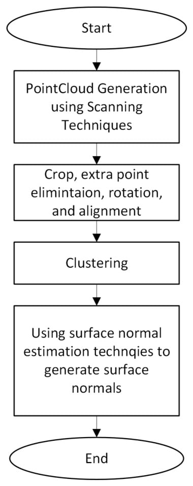
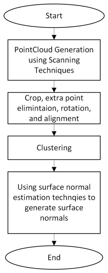
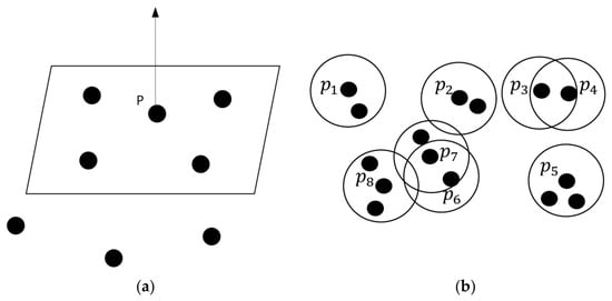
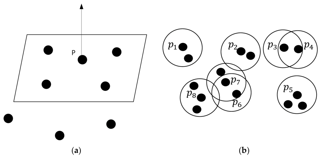
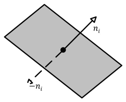
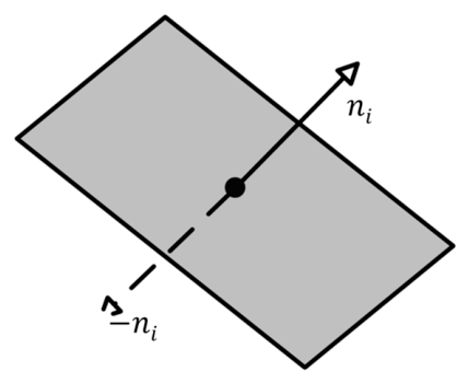
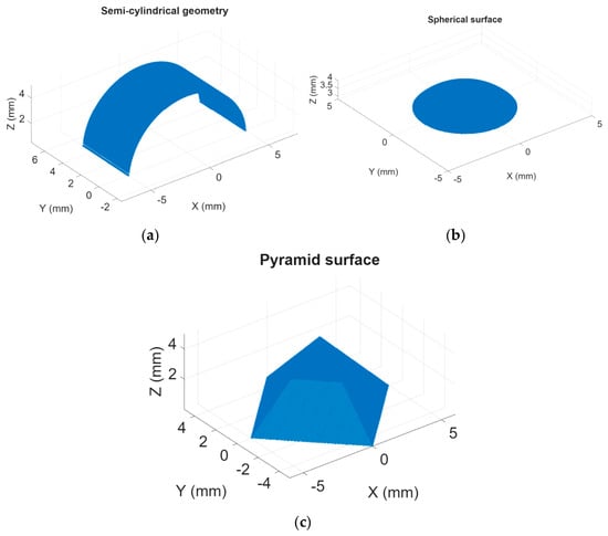
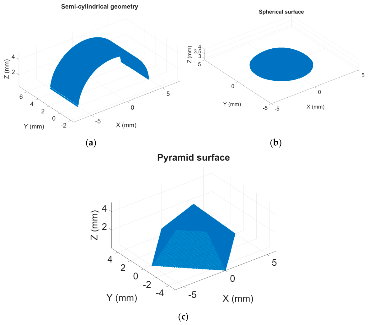
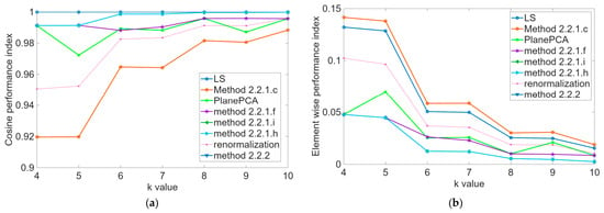
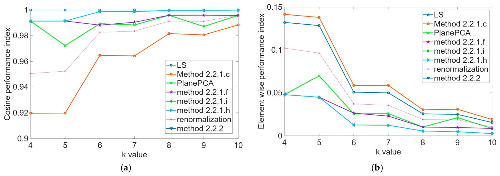
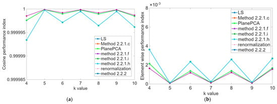
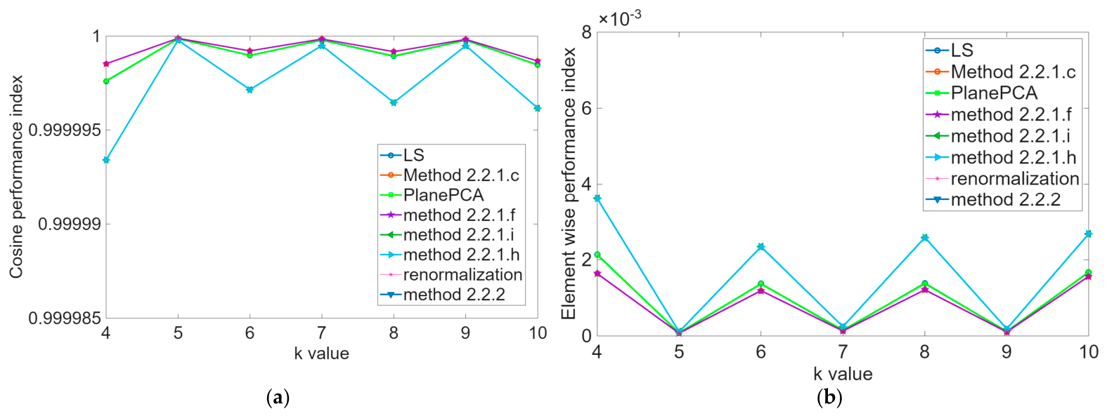
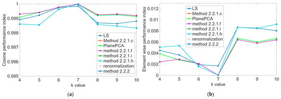
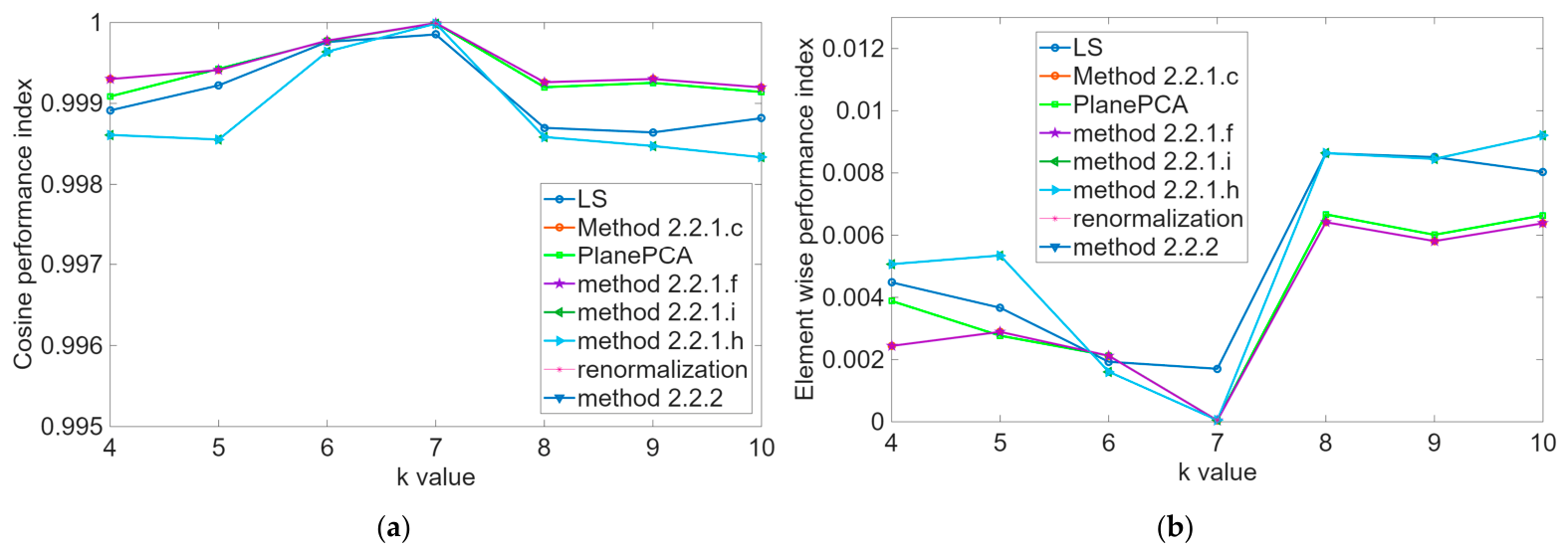
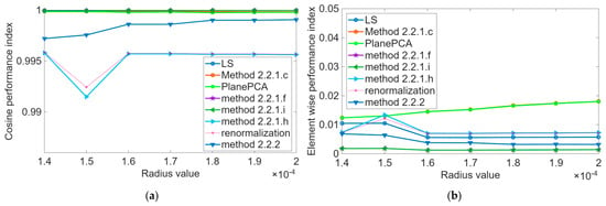
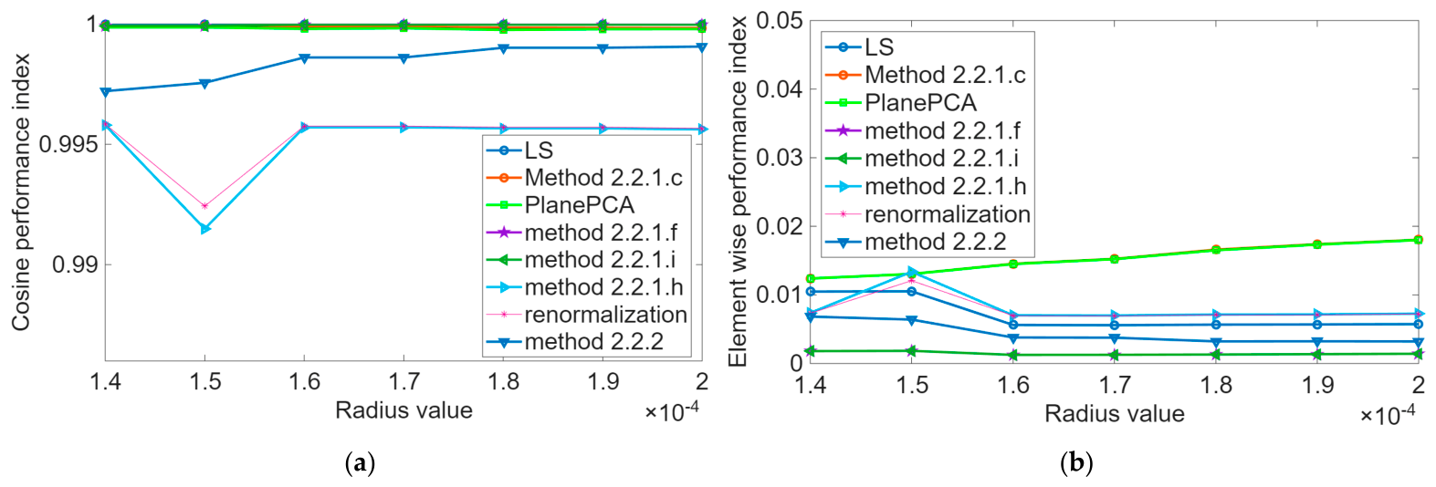
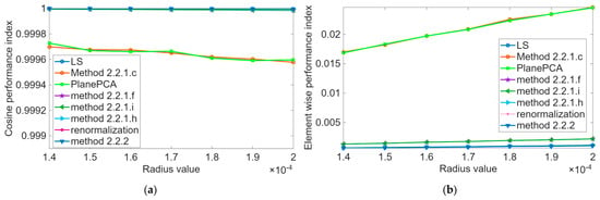
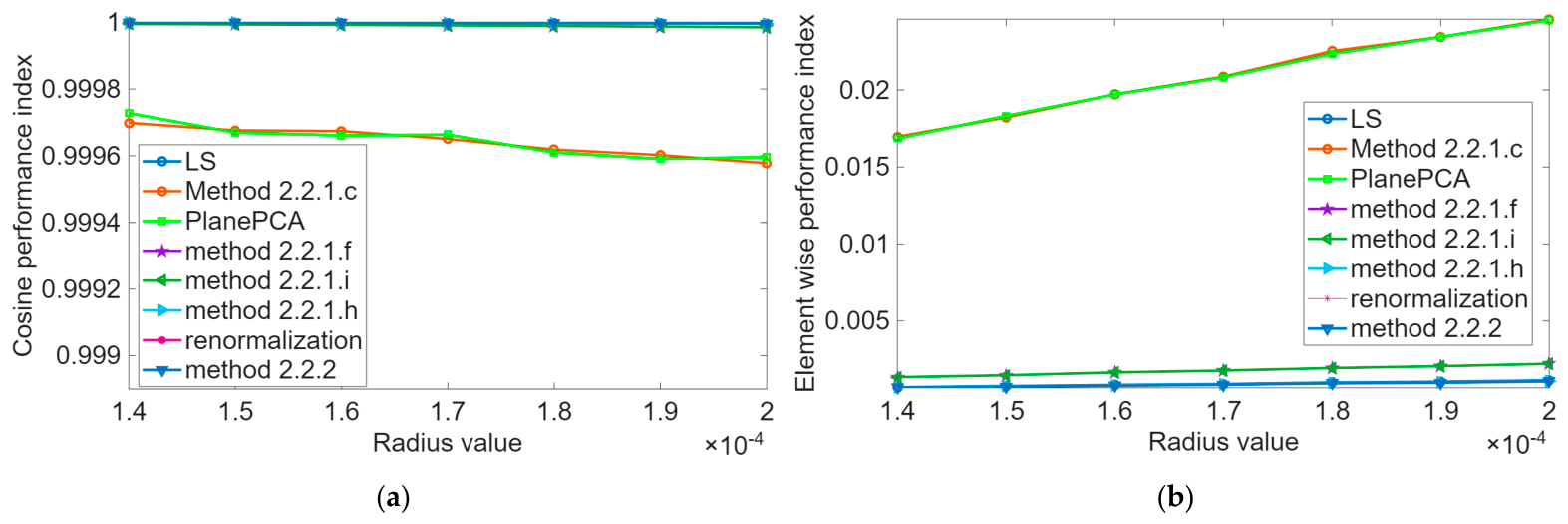
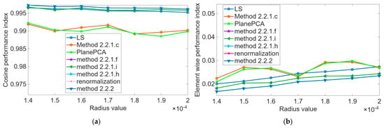
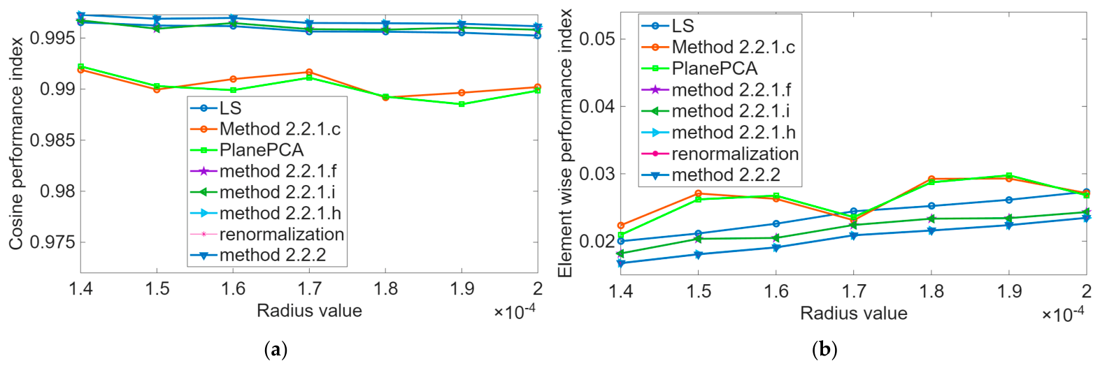
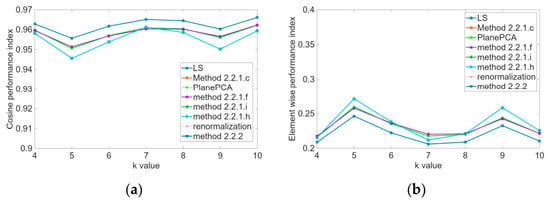
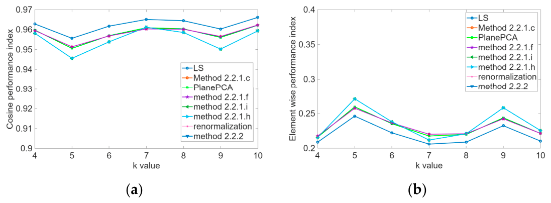
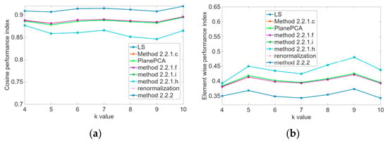
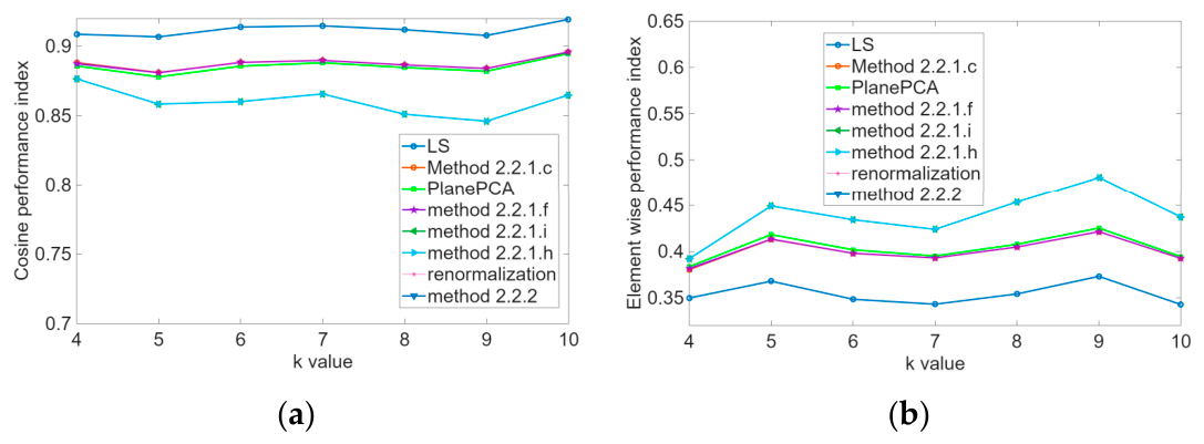
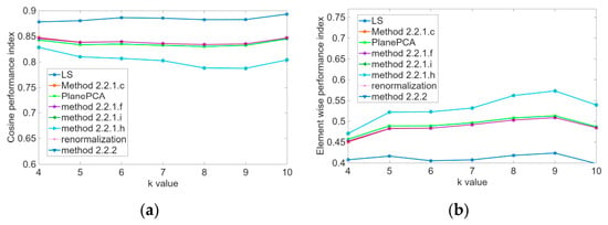
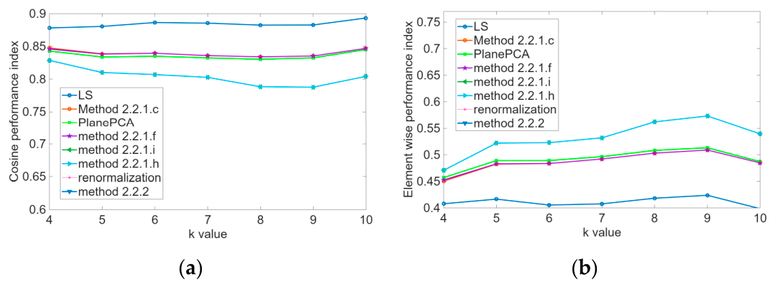
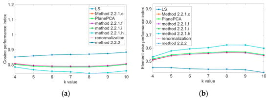
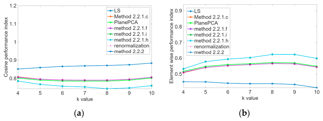
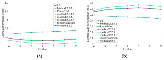
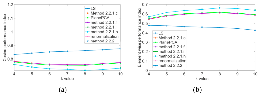
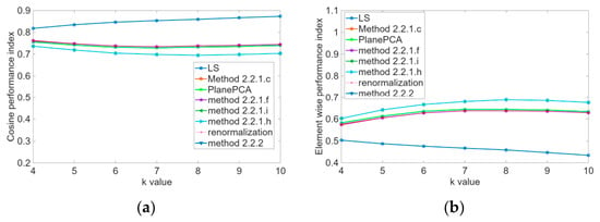
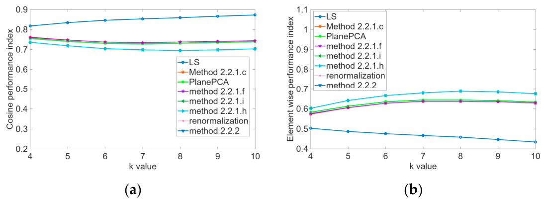
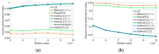
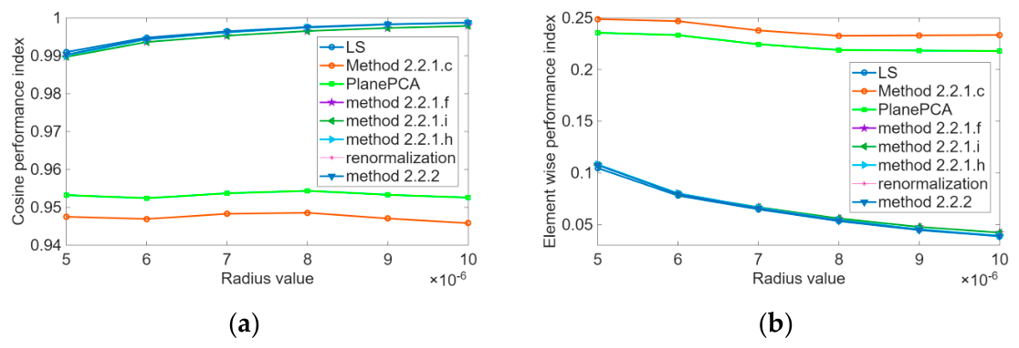
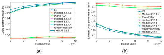
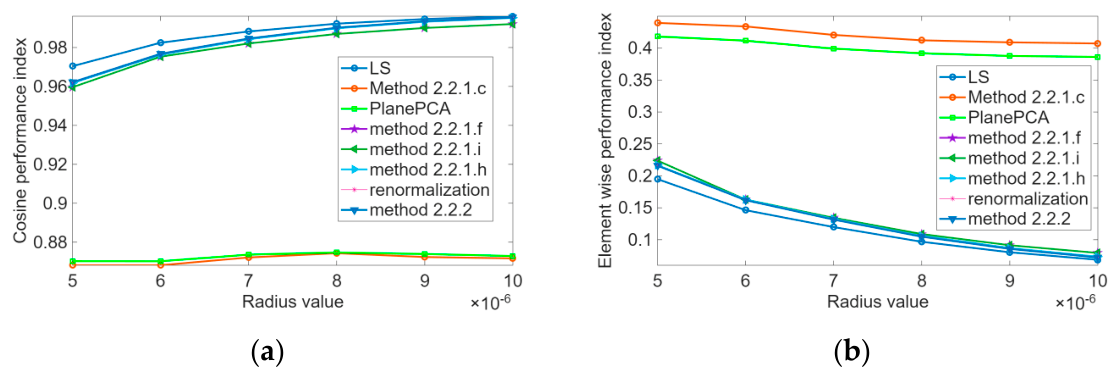
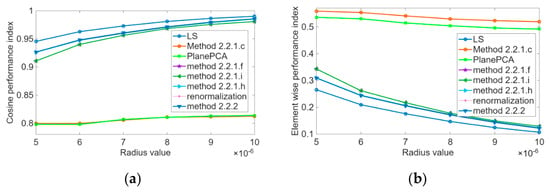
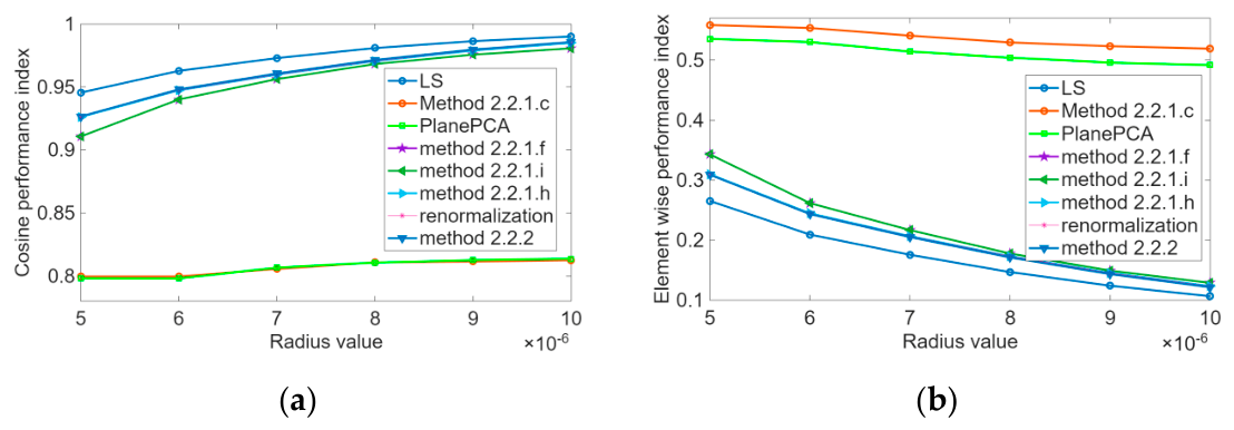
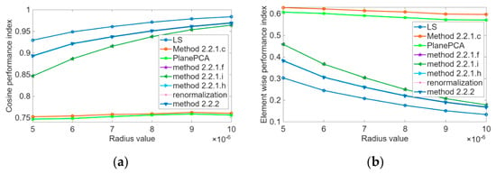
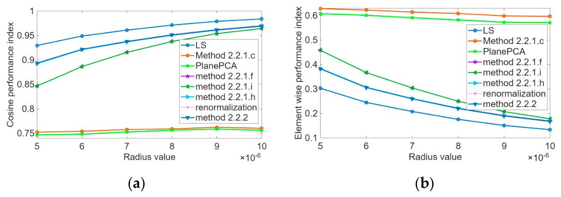
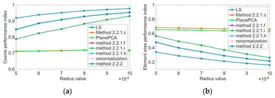
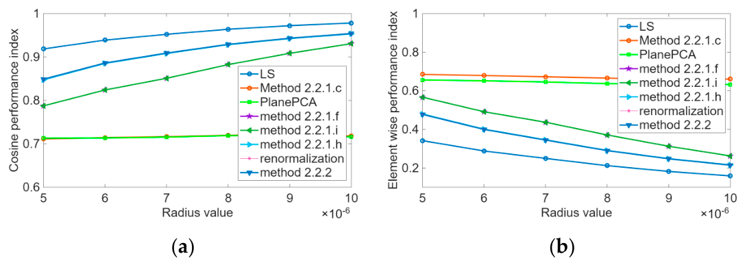
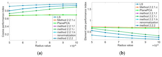
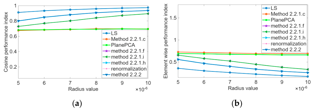
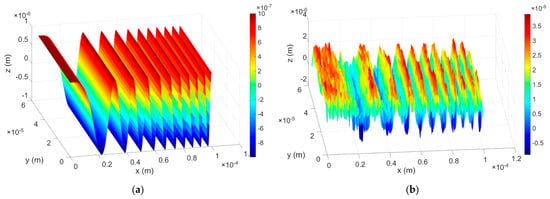
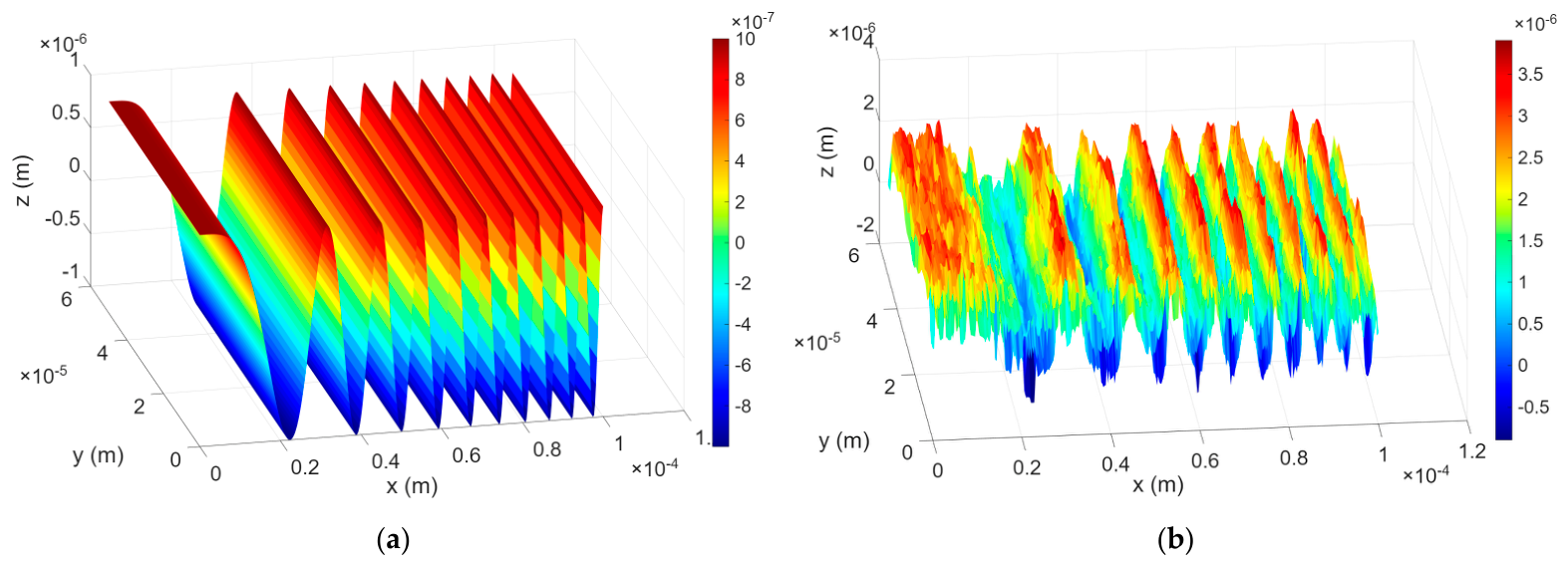
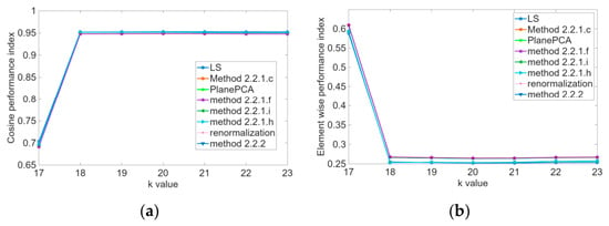
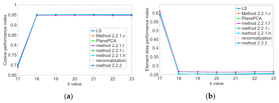
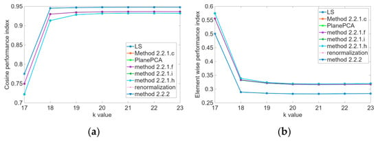
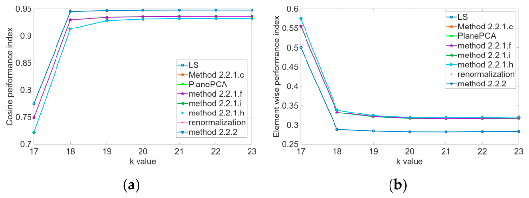
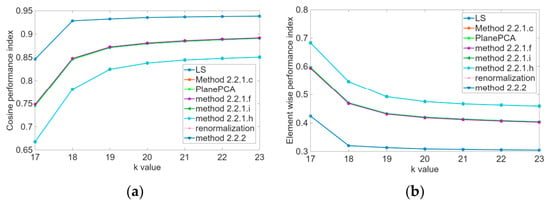
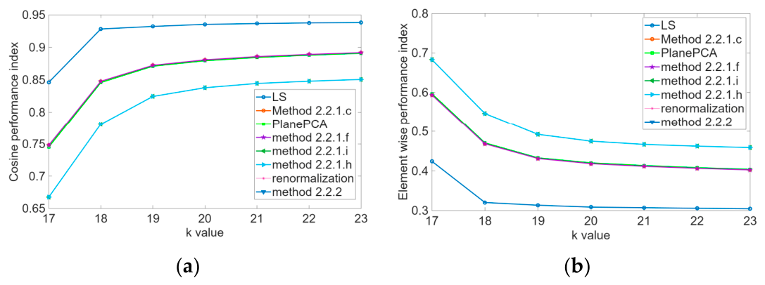
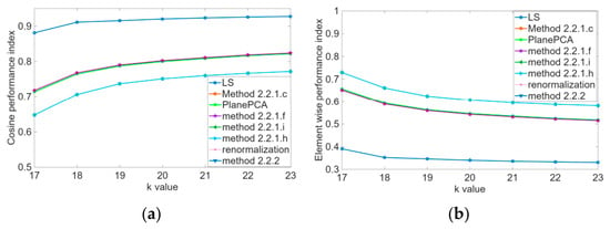
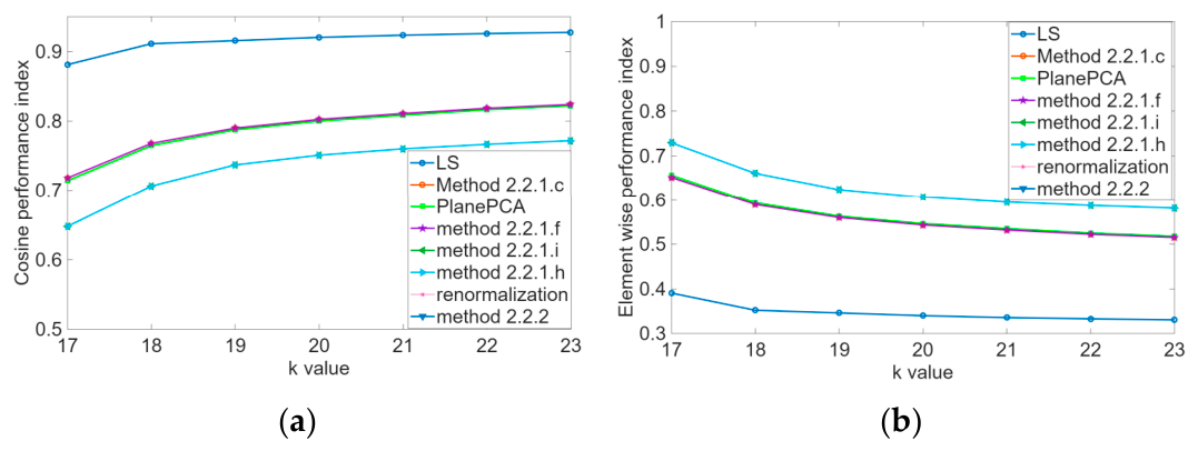
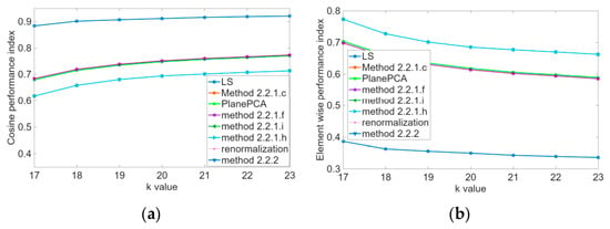
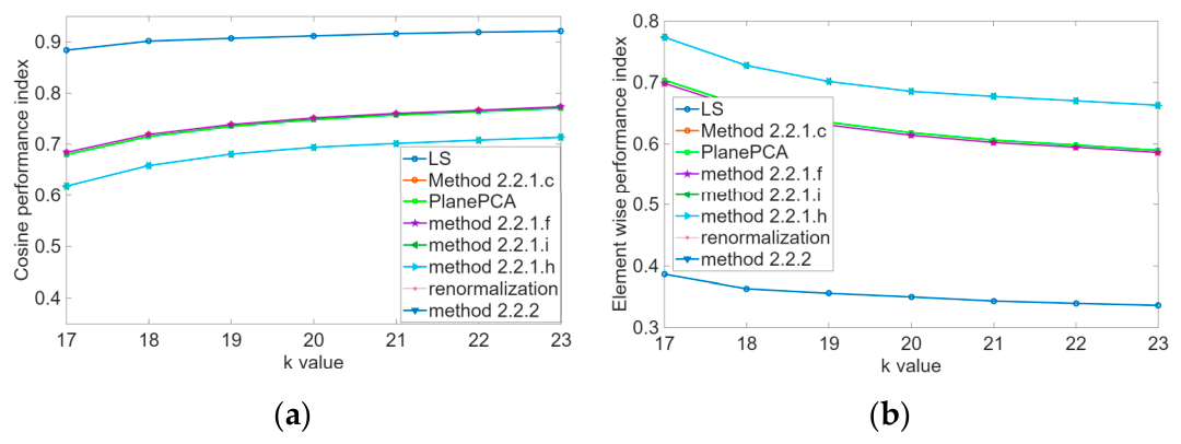
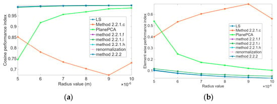
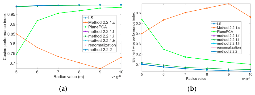
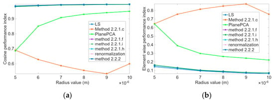
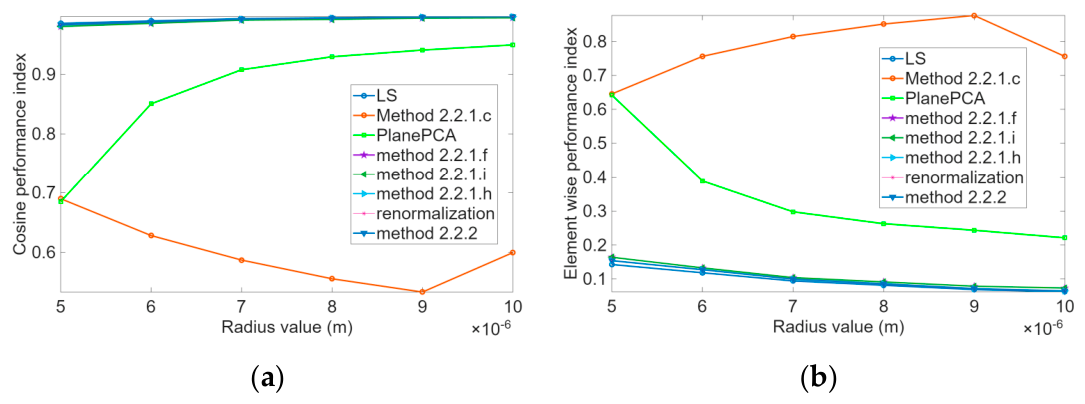
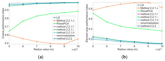
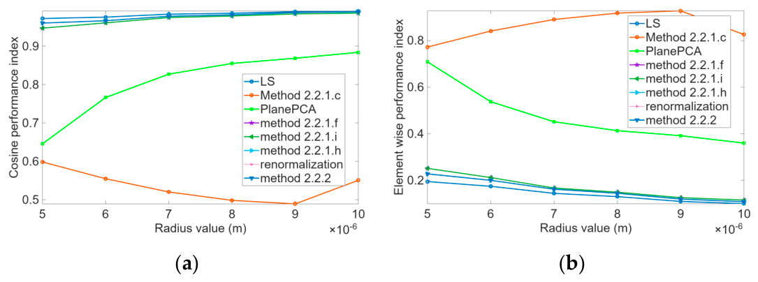
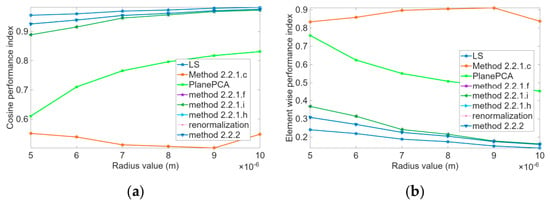
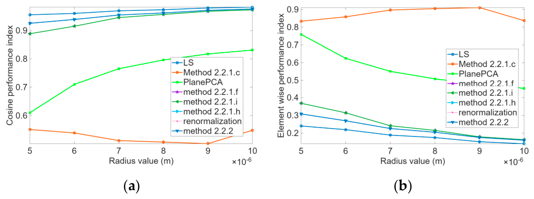
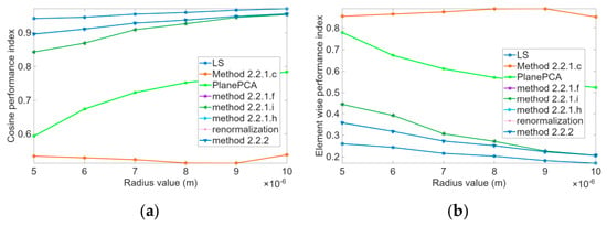
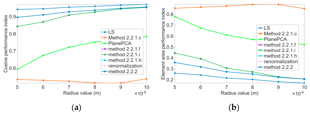
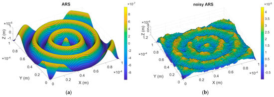
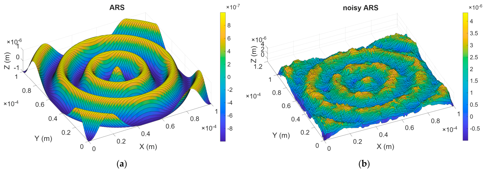
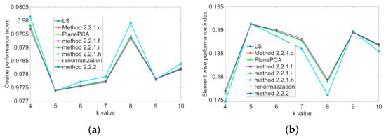
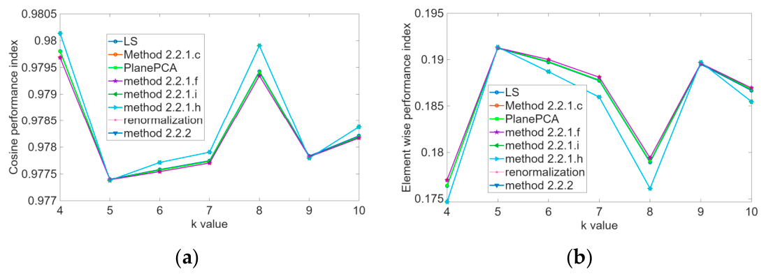
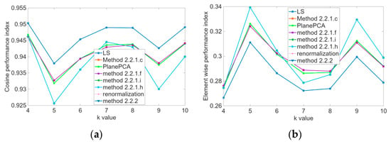
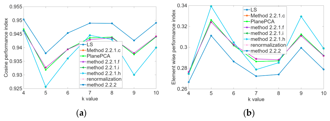
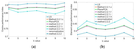
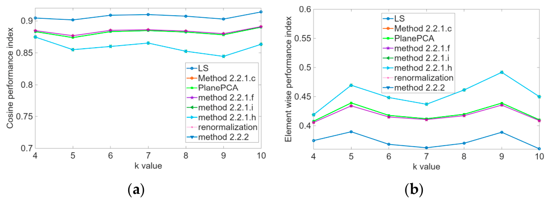
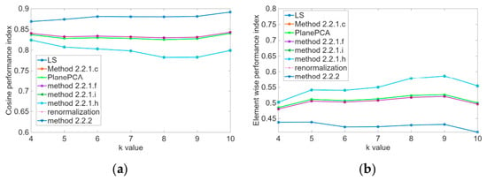
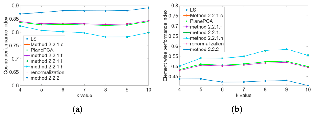
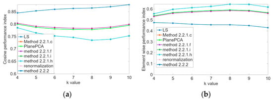
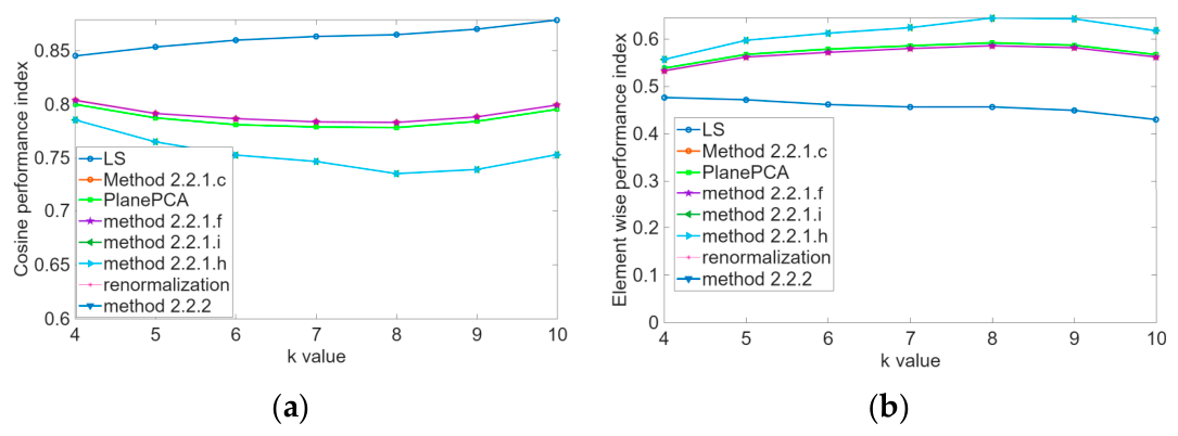
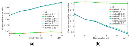
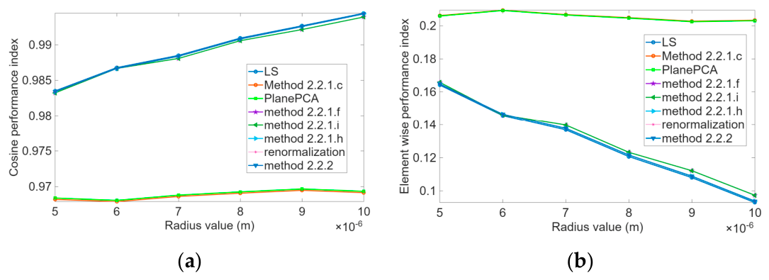
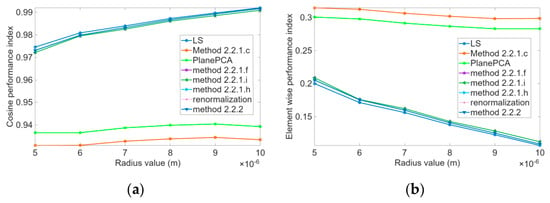
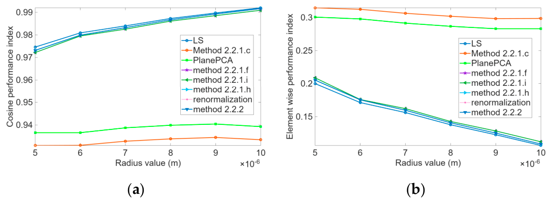
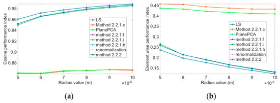
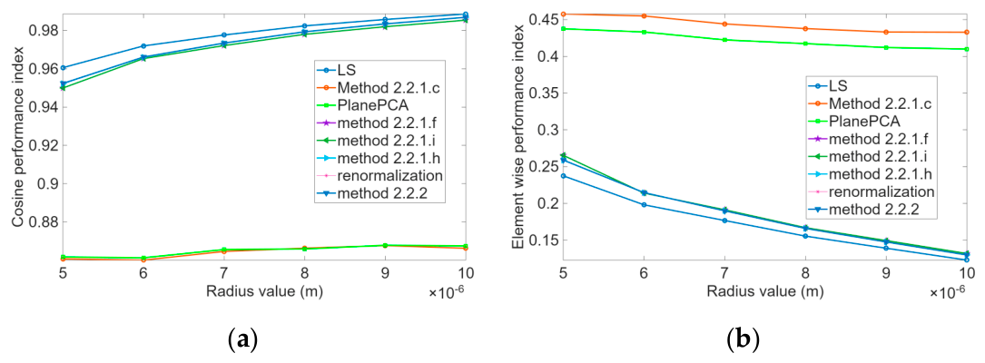
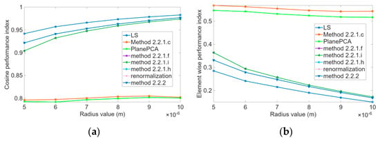
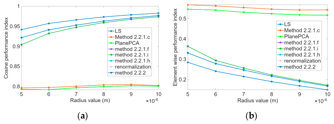
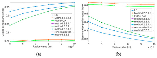
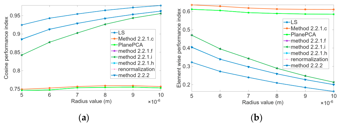
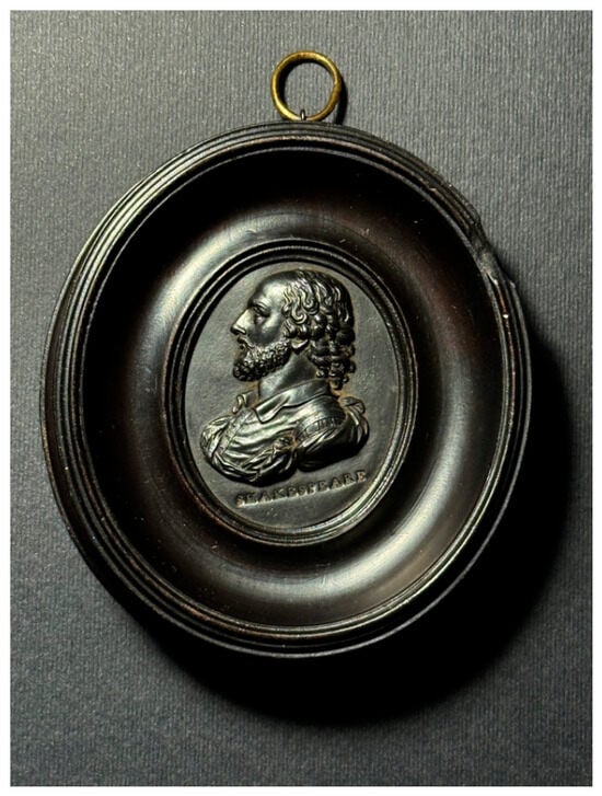
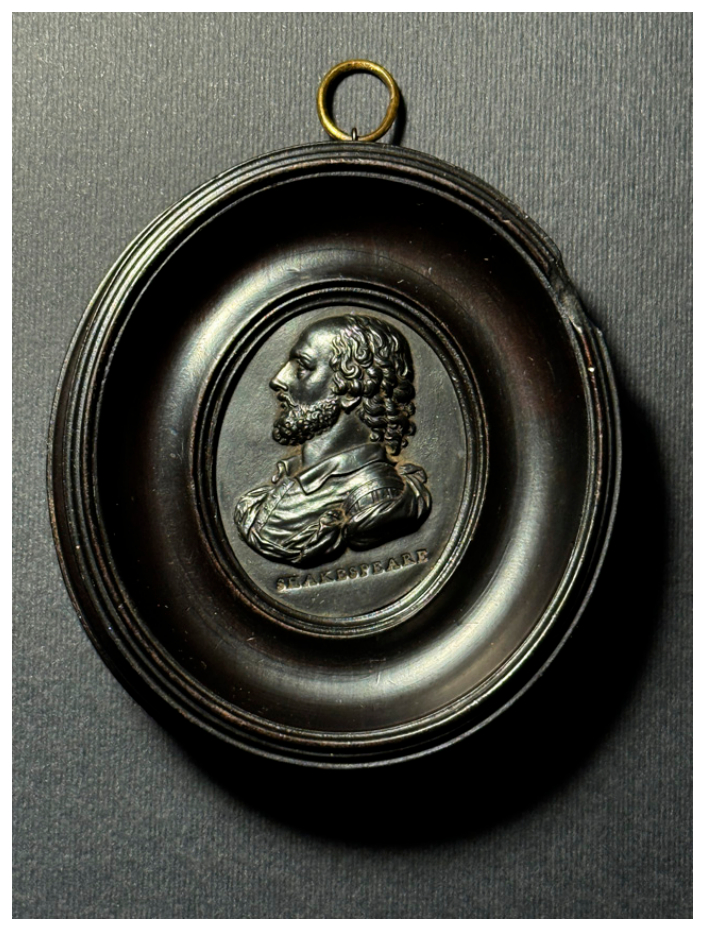
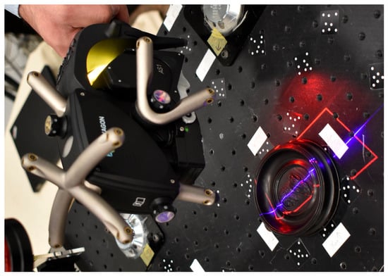
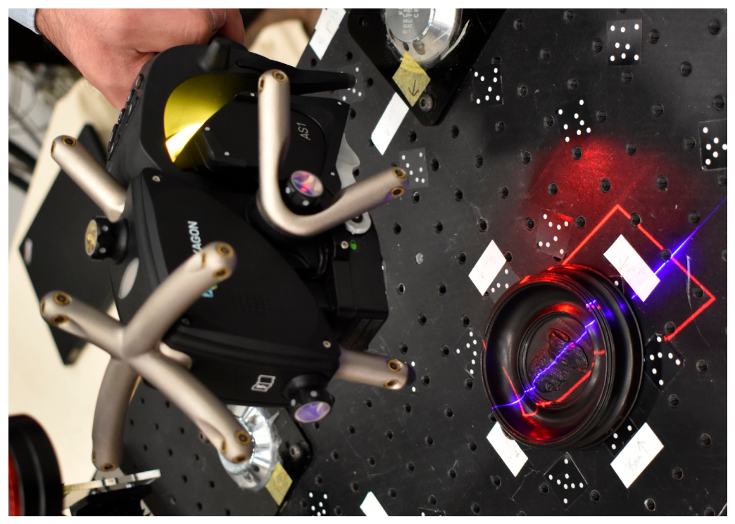
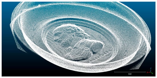
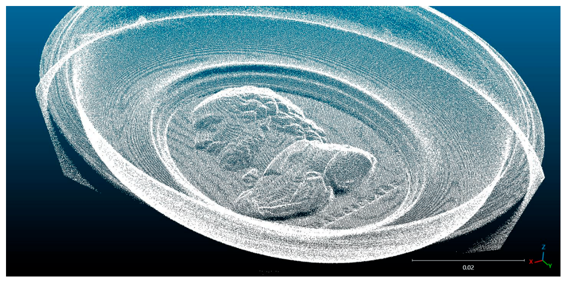
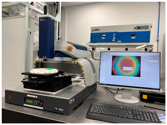
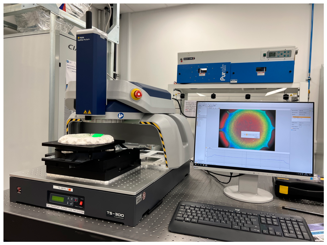
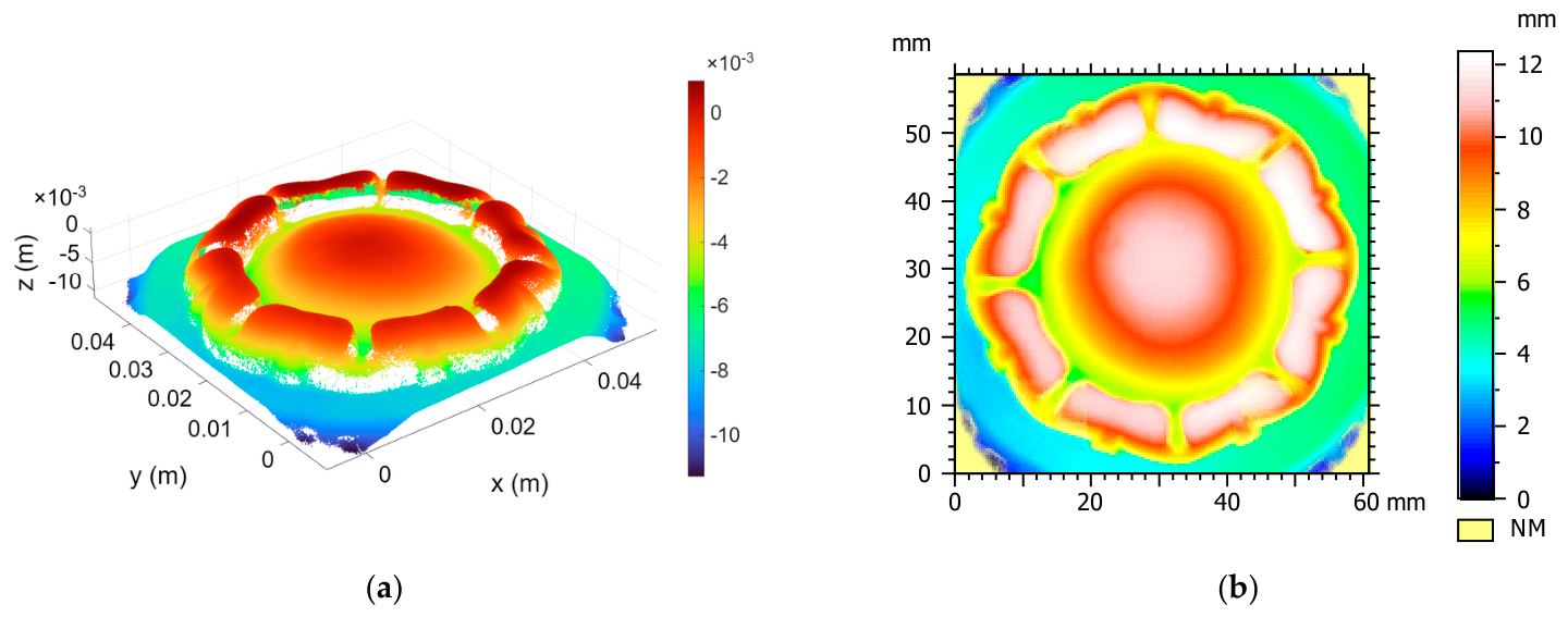
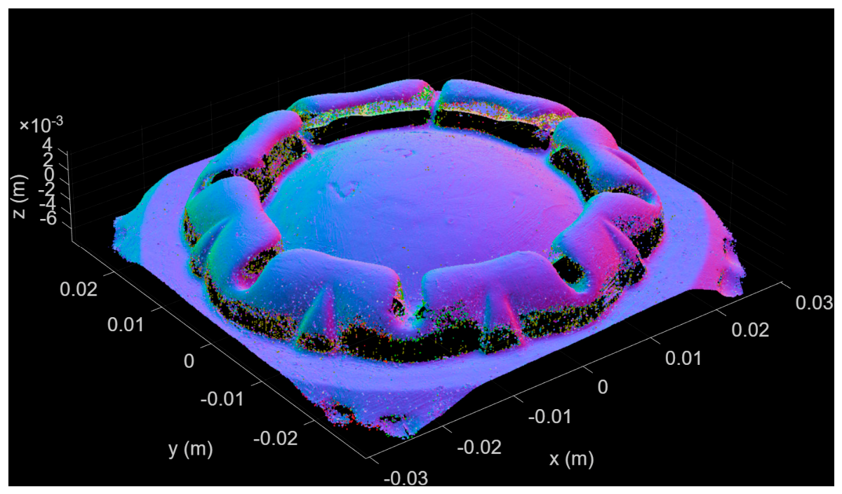
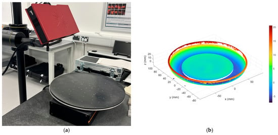
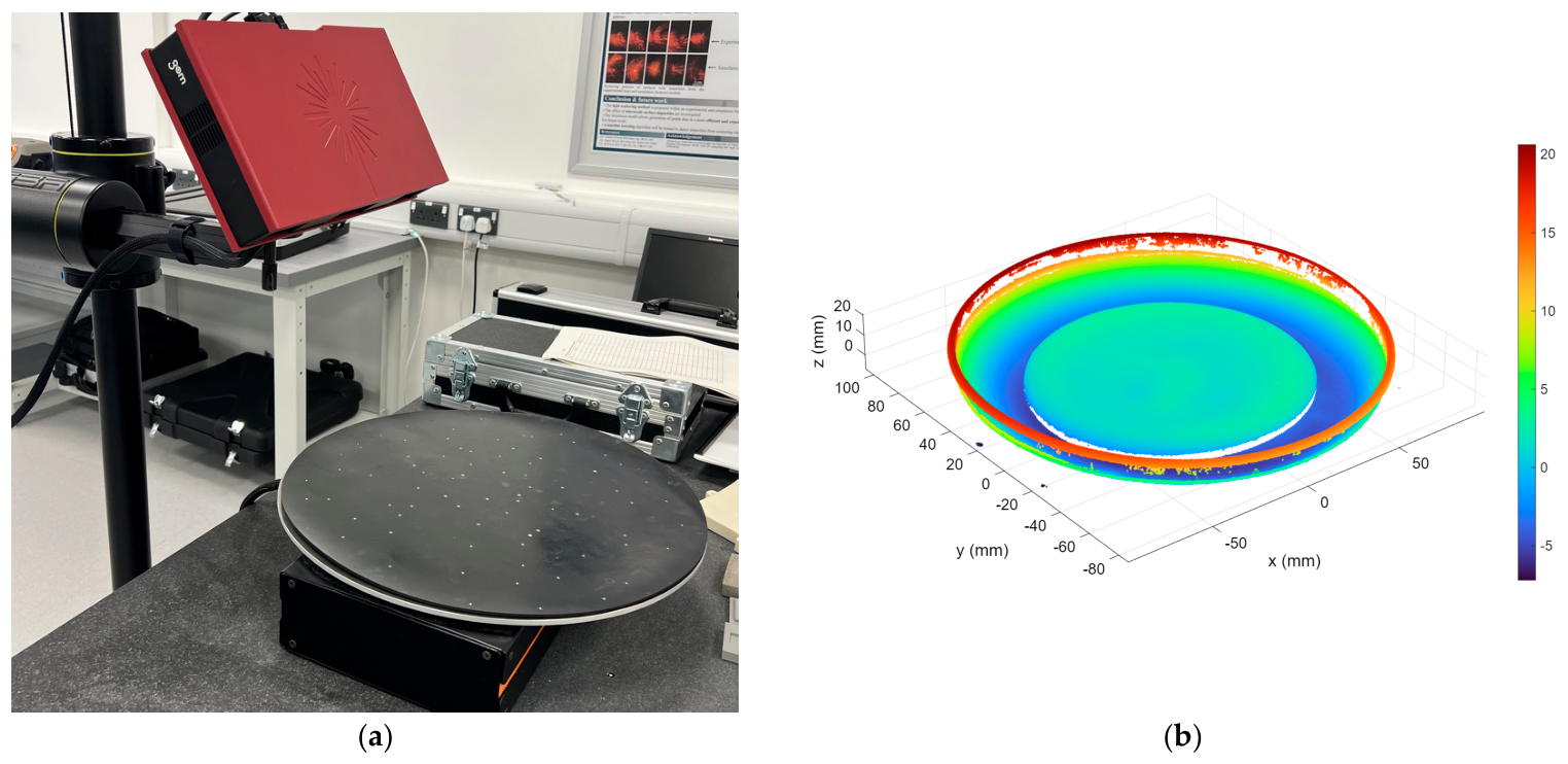
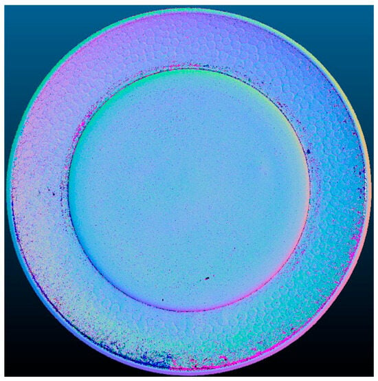
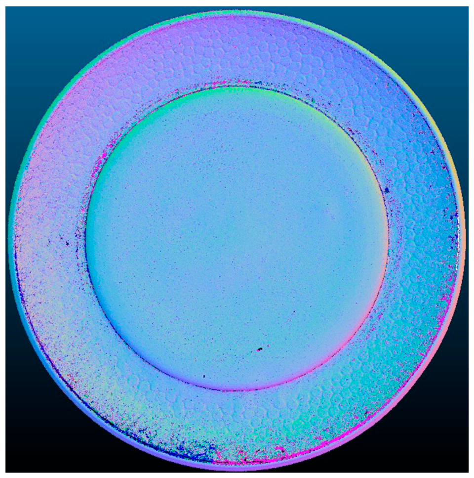
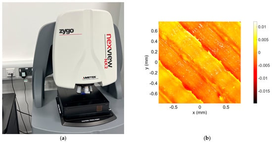
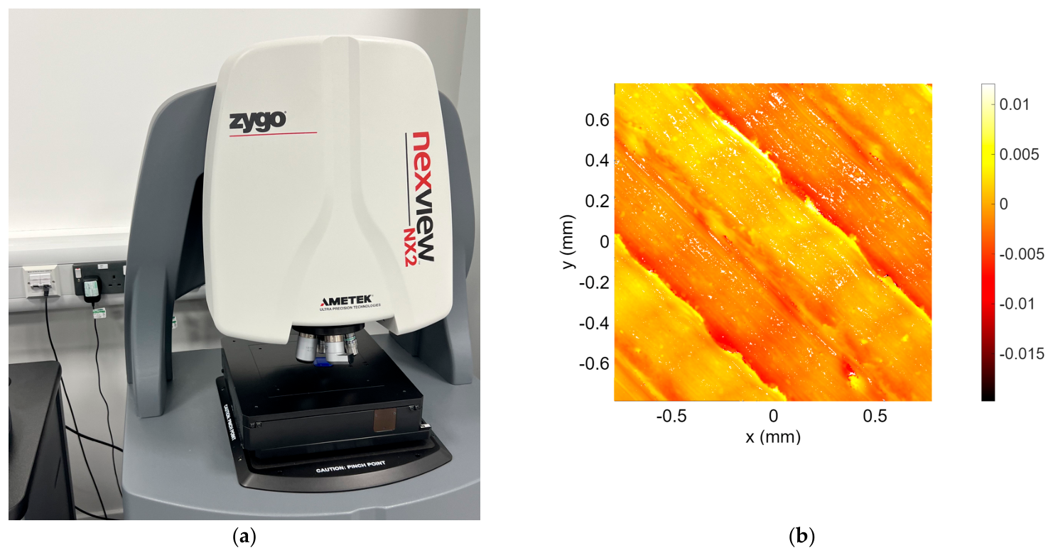
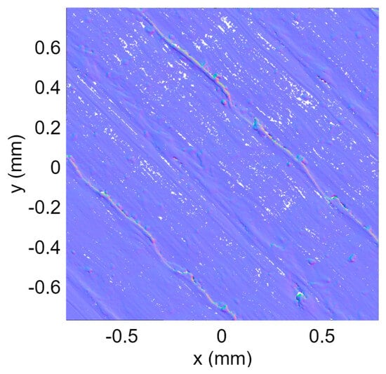
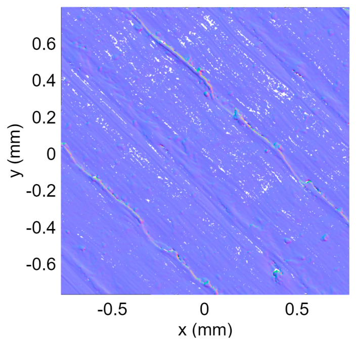
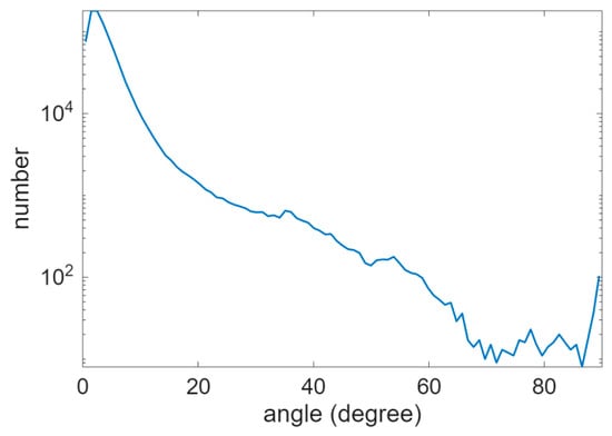
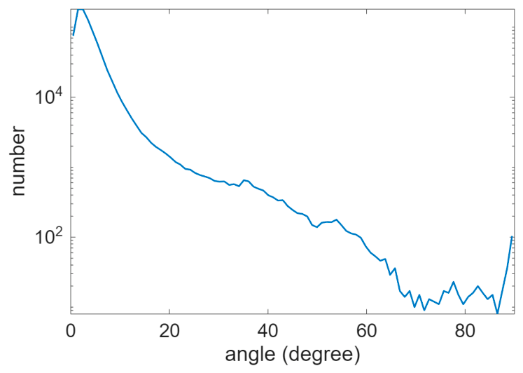
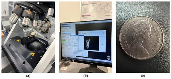
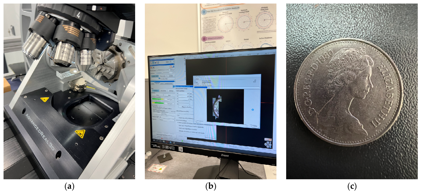
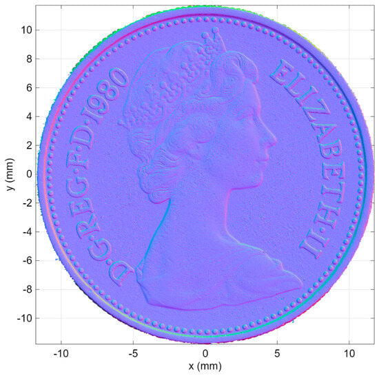
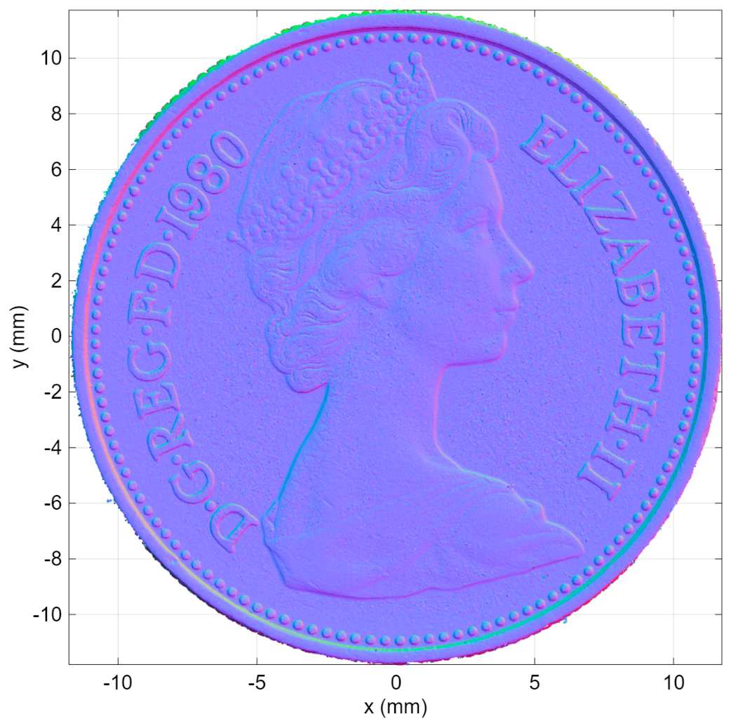
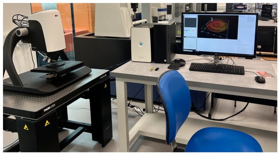
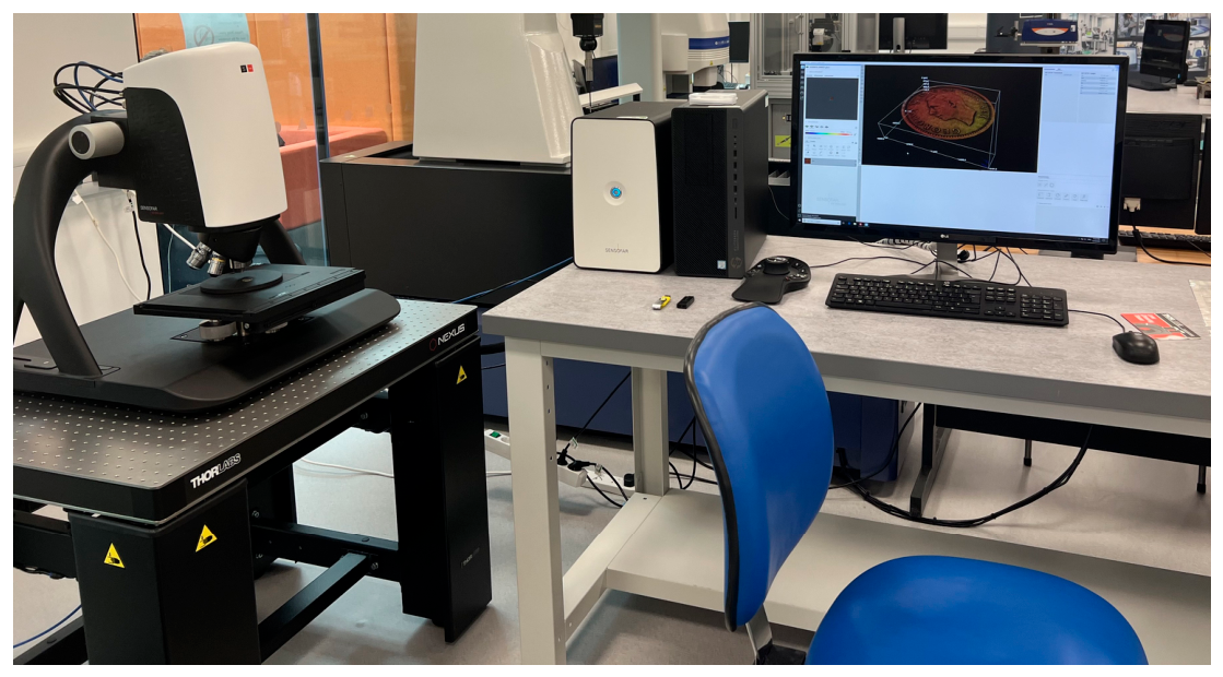
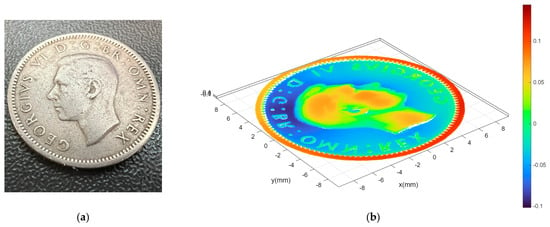
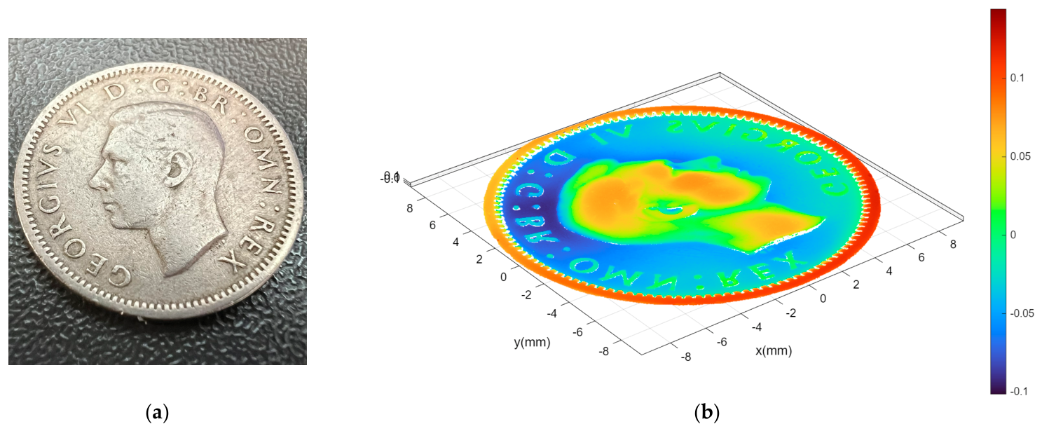
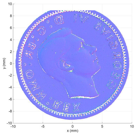
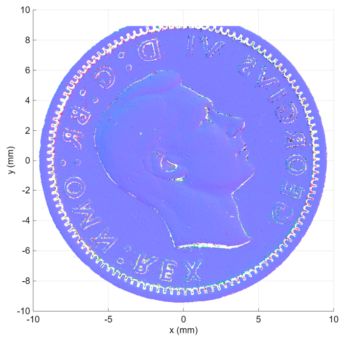

Disclaimer/Publisher’s Note: The statements, opinions and data contained in all publications are solely those of the individual author(s) and contributor(s) and not of MDPI and/or the editor(s). MDPI and/or the editor(s) disclaim responsibility for any injury to people or property resulting from any ideas, methods, instructions or products referred to in the content. |
© 2026 by the authors. Licensee MDPI, Basel, Switzerland. This article is an open access article distributed under the terms and conditions of the Creative Commons Attribution (CC BY) license.