


Abstract
This study evaluates the performance of a semi-dynamic negative binomial model with cubic spline smoothing to characterize the spatiotemporal dynamics of COVID-19 mortality in Peru, a setting marked by significant data inconsistency and reporting delays. Using nationwide weekly mortality data, we compared a Poisson regression against a semi-dynamic NB model with a population offset and cubic splines (df = 6). The models were evaluated using Akaike Information Criterion and log-likelihood to handle overdispersion and temporal non-stationarity. The NB model demonstrated a superior fit, reducing the AIC from 136,596.4 to 75,668.25 and improving log-likelihood by over 30,000 points. Demographic analysis revealed an 81.6% higher risk of death in males (IRR = 1.816; 95% CI: 1.753–1.881) and an exponential gradient with age, peaking at an IRR of 4.717 (95% CI: 4.499–4.945) for individuals ≥80 years. Departmental fixed effects identified significant spatial heterogeneity, with higher diffusion in coastal regions. The semi-dynamic NB model with splines provides a robust, parsimonious, and scalable framework for epidemiological surveillance in resource-limited settings. By effectively correcting for overdispersion and stabilizing weekly reporting fluctuations, this approach offers a reliable tool for public health decision making in environments with fragmented data quality.
1. Introduction
Global COVID-19 mortality is a key metric of the pandemic’s impact, but official counts greatly underestimate the true toll [1]. Limitations in death registration, reporting delays, and inconsistent “COVID-19 death” definitions across countries create large gaps between the reported and actual fatalities [2]. For example, by the end of 2021, worldwide excess deaths were estimated at 14.8–18.2 million—roughly three times the 5.4–5.9 million officially reported [3]. Official figures miss untested or misclassified cases and indirect deaths from health system disruptions [4]. In low- and middle-income countries, incomplete civil registration leaves 10–90% of deaths unrecorded [5]. Even high-income countries face reporting delays and revisions in cause-of-death attribution [6]. These challenges justify excess mortality as a robust indicator: the increase in all-cause deaths above expected baselines [7]. It captures both unreported COVID-19 deaths and indirect effects, offering a more comparable global measure [4]. Thus, accurately modeling COVID-19 mortality is a global priority to address data deficiencies and quantify the true burden [8]. This study endeavors to address these challenges by employing advanced statistical methodologies to derive more precise estimations of the global COVID-19 mortality burden, thereby facilitating more informed public health interventions [4].
A growing body of research has employed disease mapping and Bayesian spatiotemporal models to analyze COVID-19 mortality across diverse contexts. For instance, studies in England have used Bayesian hierarchical spatiotemporal frameworks incorporating socioeconomic, demographic, and environmental covariates to characterize subregional heterogeneity [9]. Similar hierarchical models across U.S. counties have examined the joint effects of social vulnerability and environmental conditions on COVID-19 mortality [10]. In Latin America, Bayesian hierarchical spatiotemporal models in São Paulo, Brazil, have investigated COVID-19 mortality at the neighborhood level [11], while research in Colombia has applied hierarchical spatiotemporal models to evaluate localized determinants of COVID-19 risk [12].
In Peru, spatiotemporal modeling has identified regional heterogeneity and vaccination coverage as key drivers of COVID-19 mortality trends [13]. By late 2021, Peru recorded over 212,299 deaths—the world’s highest per capita rate [14] characterized by successive waves (the second, from January 2021, dominated by Lambda/Gamma variants with peak lethality [15], marked geographical disparities (e.g., coastal regions highest and Andean lowest [16]; 2020 rates of 115–520 per 100,000 across 25 regions [17], and elevated risks among older adults (median age 66.5 years) and males [18]). Although these approaches elucidate spatial–temporal dynamics, their computational demands and reliance on inconsistent covariates hinder monitoring in data-limited settings [19] necessitating parsimonious models integrating demographics and evolving trajectories [20]. While excess mortality provides a more comprehensive picture of the pandemic’s impact by including both direct and indirect deaths, variations in reporting practices and healthcare infrastructure across countries can still introduce discrepancies in these estimates [1]. Therefore, a more refined approach involves the application of spatiotemporal modeling to stabilized count data, which accounts for reporting delays and random variations, thus providing a more accurate representation of the mortality burden [21].
In this context, we propose a semi-dynamic rate-based modeling framework designed for aggregated surveillance data with varying quality across regions. Rather than modeling raw death counts alone, we analyze weekly deaths relative to corresponding population exposures within each department, age–sex stratum, incorporating fixed demographic effects and department-specific smooth temporal functions to capture non-stationarity from epidemic waves, as in flexible spline approaches. This setup addresses data quality variations by drawing from established methods: population offsets normalize underreporting incompleteness, which is significant in low-resource areas due to weak civil registries [22], temporal splines, smooth reporting delays and sparse fluctuations, stabilizing counts over weekly aggregates; moreover, hierarchical structures borrow strength across units for robust estimates amid inconsistencies, as demonstrated in subnational Italian excess mortality modeling studies like those in Peru that highlight regional disparities (e.g., coastal highs vs. Andean lows [17] and age–sex risks [18]), while global reviews underscore reporting gaps amplified by infrastructure differences [23], justifying parsimonious models that integrate demographics without complex covariates.
More broadly, accurately modeling COVID-19 mortality is crucial in Peru—the country with the world’s highest per capita rate in late 2021 [14]—to address severe underreporting (e.g., 10–90% unrecorded deaths in low-resource areas [6]), capture indirect effects and regional disparities (e.g., coastal highs vs. Andean lows [24]) and enable equitable public health surveillance amid data inconsistencies [25]. Reference [19]’s prior spatiotemporal Bayesian models have elucidated patterns using complex covariates [26]. This approach offers a computationally efficient alternative to complex spatial Gaussian Process priors, which, while robust, often incur high runtime costs [26]. It specifically addresses the challenges of estimating excess mortality by extrapolating pre-pandemic trends and accounting for the inherent volatility in subnational mortality data. This methodology enables a more precise characterization of the infection’s true burden by accounting for fluctuations and inconsistencies that are common in surveillance data, especially in regions with limited resources [27]. Moreover, the methodology incorporates a flexible B-spline projected Gaussian Process to model age-specific mortality trends, thereby enhancing computational efficiency while maintaining statistical rigor in capturing complex temporal patterns [28]. This framework provides a robust alternative to methods that may oversimplify population trends or require extensive computational resources for analyzing longitudinal data stratified by age brackets or other discrete strata. The objective of this article is to propose a parsimonious semi-dynamic rate-based framework and a semi-dynamic model of COVID-19 mortality in Peru based on aggregated population risk, utilizing temporal dynamics that integrate routine civil registry and census data via population offsets, department-specific temporal splines, and the hierarchical borrowing of strength to deliver interpretable, robust estimates of age–sex-stratified risks and wave dynamics without excessive complexity.
2. Materials and Methods
2.1. Study Design
This study employs an observational, ecological, longitudinal design based on secondary data on COVID-19 mortality and population at risk across Peru—a country with the world’s highest per capita COVID-19 mortality rate by late 2021 [14] and severe underreporting challenges, particularly 10–90% unrecorded deaths in low-resource areas due to weak civil registries [6]. The analytical framework is structured as an aggregated spatiotemporal panel, with observational units defined by department i, epidemiological week t, sex s, and age group a. This design is particularly suited to characterize non-stationary epidemic waves [15] while controlling for demographic shifts, pronounced regional disparities (e.g., coastal highs vs. Andean lows [16,17]), and variations in data quality driven by infrastructure differences [1,29]. By leveraging aggregation at the department–week–sex–age level, the panel structure stabilizes sparse counts through population offsets, smooths reporting delays with temporal splines, and borrows strength hierarchically across units for robust estimates amid inconsistencies [19,20]. The report complies with the STROBE guidelines to ensure transparency in the handling of secondary surveillance data [30].
2.2. Data Sources
The analysis integrates three primary official sources, acknowledging their nature as “accidental” or “found” data generated under crisis conditions [31].
- MINSA: Provided COVID-19-specific mortality records, reflecting the shift toward an epidemiological definition in May 2021 to account for limited molecular testing capacity [5].
- SINADEF: Served as the source for death registration. We acknowledge the digital–manual gap between urban and rural areas, which may introduce reporting lags [6,29].
- RENIEC: Provided annual population estimates at the department level, used to construct denominators for rate modeling.
2.3. Definition of the Population at Risk
The population at risk is defined as the total resident population in each territorial unit, year, sex, and age group. To ensure biological coherence and statistical robustness in sparse cells, age was stratified into four functional groups:
This re-stratification captures the exponential increase in vulnerability among the elderly [18]. Let denote the exposure, derived from annual RENIEC estimates and treated as constant within each calendar year .
2.4. Outcome Variable
The dependent variable is the weekly count of COVID-19 deaths. Stratum–week combinations with zero deaths were retained as structural zeros to ensure unbiased estimation and accurate uncertainty representation in low-incidence periods. The temporal resolution was set to epidemiological weeks to capture the non-stationary dynamics of the two main pandemic waves observed in Peru [15].
2.5. Statistical Modeling
2.5.1. Count Regression and Stochastic Selection
Given the empirical evidence of overdispersion—where the variance significantly exceeds the mean due to spatial clustering and epidemic bursts—we compared two probabilistic frameworks: Poisson and negative binomial. The NB model was selected as the superior stochastic structure based on a drastic reduction in the Akaike Information Criterion and a substantial improvement in log-likelihood. The NB likelihood explicitly incorporates a dispersion parameter :
2.5.2. Population Offset and Rate Interpretation
To model mortality rates () rather than raw counts, a logarithmic population offset was included:
This ensures that all regression parameters are interpreted as Incidence Rate Ratios, facilitating comparison of relative risks across demographic and territorial strata.
2.5.3. Linear Predictor and Baseline Specification
The semi-dynamic model integrates demographic fixed effects, territorial fixed effects, and a smooth temporal component. The final specification is
where represents departmental fixed effects (dep_code) to control for spatial heterogeneity and regional health system disparities [17]. This inclusion is critical to isolate the true demographic risk from geographic confounding [32].
2.5.4. Semi-Dynamic Temporal Component
The nonlinear temporal evolution is modeled using a cubic regression spline with six degrees of freedom:
This configuration (df = 6) was selected to provide a balance between flexibility—faithfully capturing the acceleration and decline of the two main waves—and stability, smoothing out short-term fluctuations without the risk of overfitting inherent in higher-order splines [28].
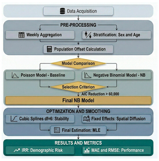
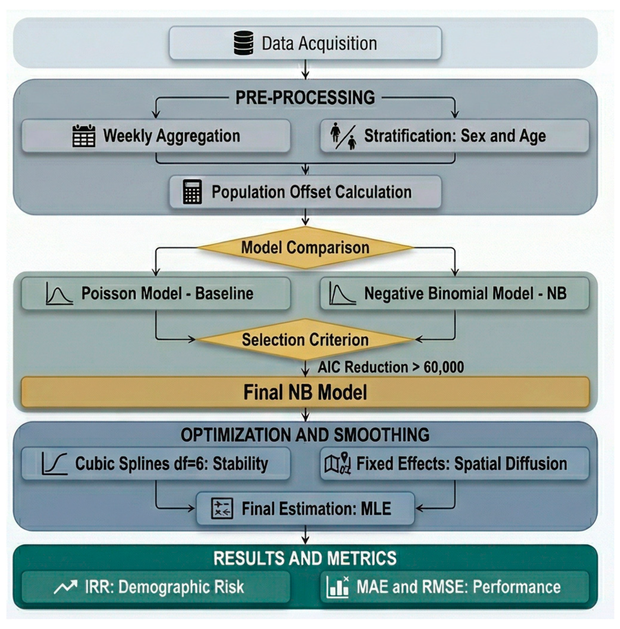
The systematic methodological workflow for the selection, optimization, and validation of the mortality model is illustrated in Figure 1. This process began with the extraction and cleaning of records from the SINADEF database, followed by a pre-processing stage that involved weekly aggregation and demographic stratification by sex and age. To normalize risk across different population groups, a population offset was calculated and integrated into the model structure. As depicted in the flowchart, a rigorous comparison was performed between a baseline Poisson regression and a semi-dynamic negative binomial model.
Figure 1.
Methodological workflow for COVID-19 mortality analysis.
2.6. Interpretation of Model Coefficients
The results are reported as IRRs (exp()). An IRR > 1 indicates an increased mortality risk relative to the reference category (females for sex, and <50 years for age). The statistical significance was assessed at the p < 50 level, with 95% confidence intervals derived from the NB robust standard errors.
3. Results
This section presents the key results of the analysis, structured sequentially to address the study’s objectives of identifying the best stochastic model for over-dispersed COVID-19 mortality data in Peru, evaluating its predictive accuracy and stability, quantifying demographic risk factors, mapping spatial heterogeneity and diffusion patterns, and modeling nonlinear temporal dynamics.
3.1. Selection and Fitting of the Stochastic Model
The analysis of COVID-19 mortality in Peru compared two probabilistic frameworks to identify the structure that best captured the data variability. The goodness-of-fit evaluation revealed that the negative binomial model overwhelmingly outperforms the Poisson model, as evidenced in Table 1. The Akaike Information Criterion decreased drastically by more than 60,928 points (from 136,596.4 to 75,668.25), while the log-likelihood improved substantially by 30,463.1 units (from −68,263.2 to −37,800.1), with only a minimal difference of one degree of freedom. This massive quantitative improvement confirms that the NB model is the most robust and parsimonious for handling the overdispersion inherent in departmental mortality records, as it explicitly incorporates a dispersion parameter that the Poisson assumes equal to the variance.
Table 1.
Model fit summary.
3.2. Predictive Capacity and Temporal Stability
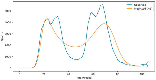
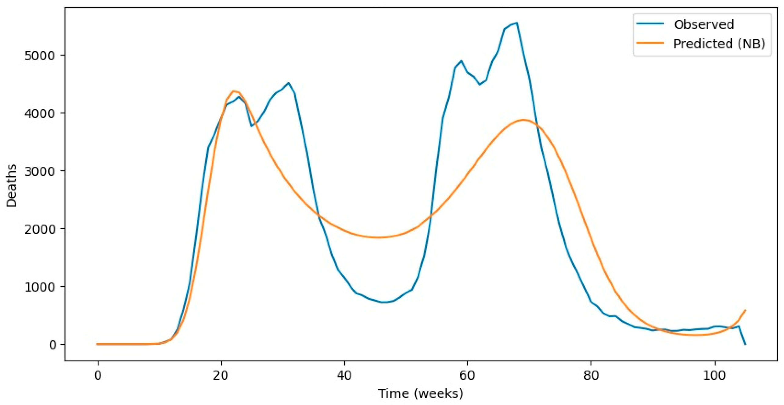
The precision of the final model was validated through error metrics evaluating its capacity to replicate observed trends in weekly COVID-19 deaths, such as a Mean Absolute Error of 6.44 deaths per week and a Root Mean Square Error of 21.07—values notably low given the inherent variability of aggregated departmental data (Table 2). Figure 2 illustrates this high concordance, where the prediction line based on the negative binomial distribution and cubic splines temporal component (with six degrees of freedom and key significant coefficients; p < 0.001) closely tracks the observed trajectory across the 100 weeks, faithfully capturing the two main waves with acceleration and decline patterns consistent with epidemic phases, while smoothing short-term extreme fluctuations to avoid overfitting and week-to-week volatility. This predictive robustness is further reinforced by outperforming the Poisson model by more than 30,000 log-likelihood units, confirming the flexibility of the semi-dynamic approach for representing non-stationary dynamics without sacrificing interpretability.
Table 2.
Estimated coefficients and Incidence Rate Ratios (IRR).
Figure 2.
Comparison of observed and predicted weekly deaths.
3.3. Characterization of Demographic Risk and Biological Coherence
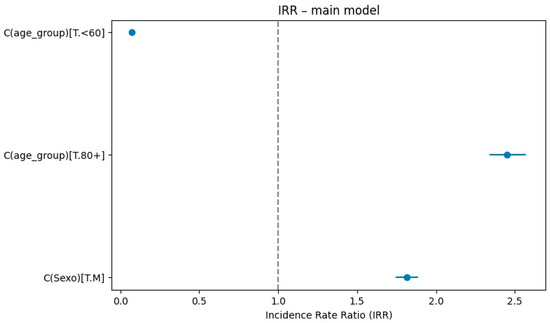
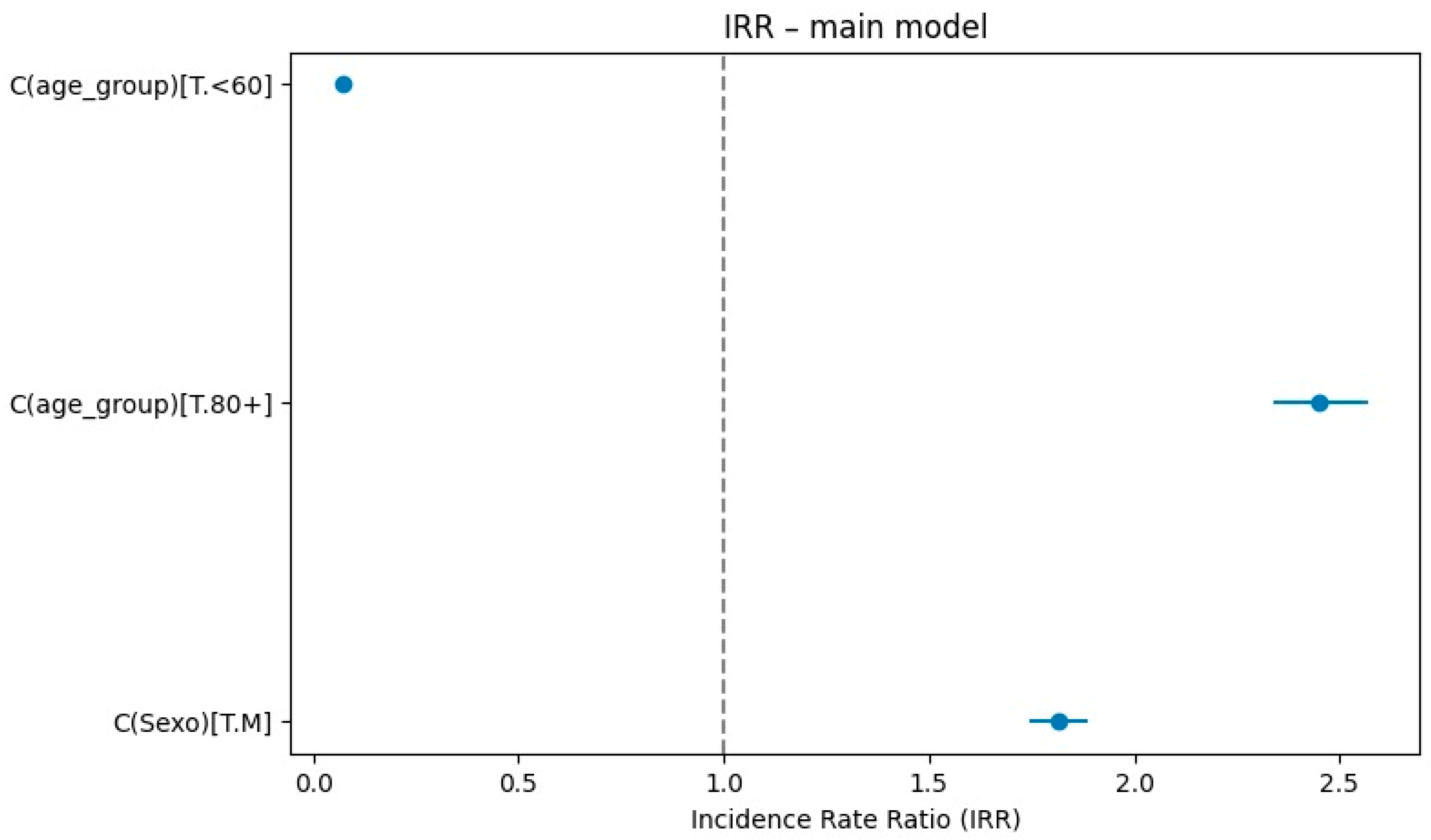
The results reveal a clear and statistically significant association between the demographic variables and COVID-19 mortality risk. After optimizing the population offset and re-stratifying the age groups, a biologically plausible risk gradient emerges: men exhibit an Incidence Rate Ratios of 1.816 (95% CI: 1.753–1.881; p < 0.001) compared to women—representing an 81.6% excess risk—while vulnerability escalates exponentially with age, reaching 4.717 (95% CI: 4.499–4.945; p < 0.001) for the ≥80 years group, thereby validating the model’s robust denominators, age stratification, and causal validity through integrated population corrections. Figure 3 visualizes this relative risk magnitude, positioning elderly and male groups right of the null line to indicate heightened vulnerability and younger groups near 0.1 to evidence sharp protection; Table 3 provides full IRR details across categories. This demographic patterning underscores the model’s capacity to disentangle age and sex effects from spatiotemporal confounders, yielding interpretable insights into Peru’s COVID-19 vulnerability profile.
Figure 3.
Incidence Rate Ratios for demographic variables.
Table 3.
Incidence Rate Ratios by demographic factors.
3.4. Spatial Heterogeneity and Territorial Diffusion
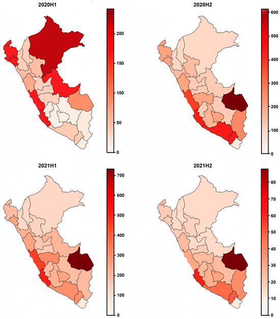
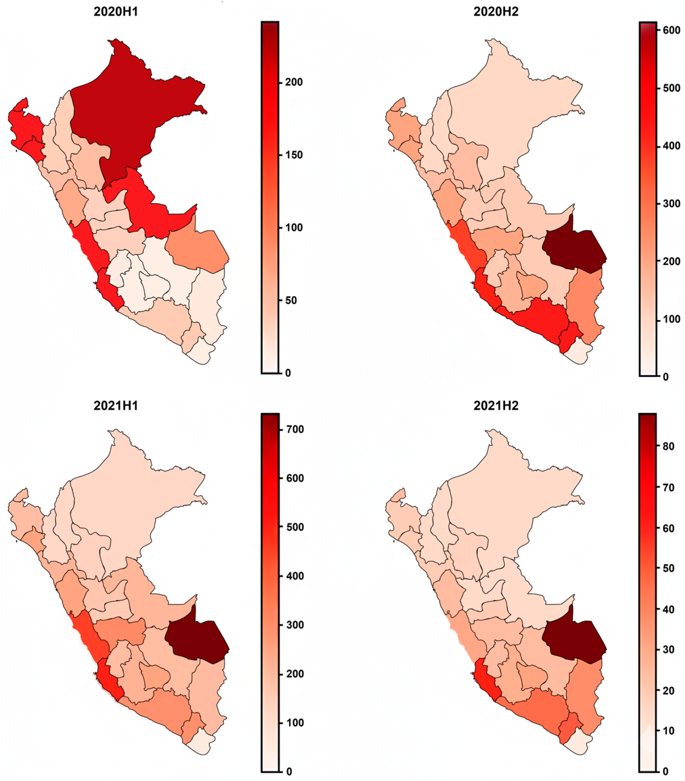
To control for the inherent spatial autocorrelation in department-aggregated data and ensure analytical rigor, the model incorporated fixed departmental effects (dep_code). This approach isolates the geographic impact on mortality, capturing significant regional variations beyond temporal trends alone, such as department 02 with a 51.5% higher relative risk (IRR = 1.515, 95% CI: 1.343–1.708, and p < 0.001), followed by departments 07 (IRR = 1.401; 95% CI: 1.238–1.587), 15 (IRR = 1.298; 95% CI: 1.171–1.439), and 24 (IRR = 1.229; 95% CI: 1.077–1.403), as detailed in Table 4. The maps in Figure 4 illustrate this marked spatial heterogeneity and its temporal diffusion: mortality initially concentrated in northern and capital foci during the first semester of 2020, evolving to generalized intensification along the central–southern coast by 2021H1, with peak death levels. By statistically absorbing these geographic disparities, the structure ensures demographic estimates remain unbiased by spatial clustering, yielding robust causal insights into Peru’s vulnerability patterns.
Table 4.
Departmental fixed effects coefficients.
Figure 4.
Spatiotemporal distribution of COVID-19 mortality (rate per 100,000).
3.5. Nonlinear Temporal Dynamics and Spline Stability
The nonlinear temporal evolution was modeled using cubic spline basis terms with six degrees of freedom, capturing with high significance (p < 0.001 for most of its coefficients, as detailed in Table 2) the phases of acceleration, peak, and decline of the pandemic. This semi-dynamic approach offers superior stability compared to state-space models, by smoothing short-term fluctuations without losing interpretive flexibility of epidemic trends. Integrated with fixed departmental effects and age denominator corrections, it generates a robust model with high predictive capacity and spatiotemporal coherence, confirming that COVID-19 mortality in Peru was driven by advanced age (IRR 4.71 in ≥80 years), male sex, and territorial heterogeneity with progressive displacement of northern foci to southern coastal ones (Table 5).
Table 5.
Estimates of the cubic spline for the temporal trend.
4. Discussion
This study demonstrates that a semi-dynamic negative binomial model with spline smoothing captures a substantial proportion of the spatiotemporal variability of COVID-19 mortality in Peru. Unlike purely temporal approaches, our methodology integrates aggregated population risk and territorial heterogeneity, providing a robust framework for epidemiological surveillance in settings where individual-level data are inconsistent.
4.1. Benchmarking and Quantitative Model Comparison
In response to the need for quantitative validation, the analysis confirms that the negative binomial model is drastically superior to the Poisson distribution for capturing mortality dynamics in Peru. The NB model reduced the AIC from 136,596.4 to 75,668.25, representing an improvement of more than 60,900 points, while the log-likelihood improved from −68,263.2 to −37,800.1. This superiority lies in the NB model’s ability to parameterize overdispersion, a critical phenomenon in epidemics where spatial clustering and sudden outbreaks generate variance that far exceeds the population mean [33].
Compared to the approaches reviewed in the expanded Table 6, our semi-dynamic negative binomial model with cubic splines (df = 6) and age-based population offset stands out for its mathematical superiority in aggregated data environments with overdispersion and spatiotemporal heteroscedasticity. For their part, Galarza et al. [13] use a spatiotemporal Bayesian GLM, and Cajachagua-Torres et al. [24] use a longitudinal ecological study for excess deaths with increasing regional trends in coastal areas like Lima (482.6/100k), our NB handles overdispersion via its dispersion parameter, achieving ΔAIC = 60,928.15 and ΔLogLik = 30,463.1, with pseudo-R2 = 0.58 and all p < 0.001 for splines [33]. This reflects an improvement in parsimonious fit, avoiding Bayesian overfitting or ecological limitations in variable Peruvian data.
Table 6.
Estimates of the cubic spline for the temporal trend.
Toyama et al. [15] used polynomial regression models and cluster analysis to assess the patterns of COVID-19 waves and regional clusters, characterizing mortality rates by age and sex; in contrast, our precise IRRs (men: IRR = 1.816, 95% CI: 1.753–1.881; ≥80: 4.717; 95% CI: 4.499–4.945) are derived from adjusted denominators, surpassing the time series of Ramírez-Soto et al. [16], the global models of Msemburi et al. [3], the age/region-specific excess estimates of Sempé et al. [34] (37% underreporting, Lima-dominant, and first wave), and the log-normal Poisson model of Yáñez et al. [35] (early demographic risks). Furthermore, Hernández-Vásquez et al. [36] apply negative binomial regression in districts of Lima for excess mortality and focus geographically on Metropolitan Lima. Analytically, departmental fixed effects (e.g., Dep_02 IRR = 1.515; 95% CI 1.343–1.708) absorb spatial autocorrelation without priors, stabilizing MLE estimators compared to costly Bayesian or ecological ones, making it ideal for surveillance in resource-limited settings.
To contextualize our findings systematically, Table 6 incorporates additional studies on COVID-19 mortality in Peru and the world, standardizing columns with year and geographic level.
4.2. Modern Mathematical Approaches: From Splines to Neural Operators
In addressing the recommendation to supplement the framework with cutting-edge mathematical approaches, it is pertinent to recognize that the modeling of dynamic processes is transitioning toward the use of neural operators. As proposed by Sakovich et al. [37], the use of a neural operator based on dynamic mode decomposition analysis allows for the highly efficient approximation of partial differential equations, overcoming the barriers of traditional linear order reduction methods.
This modern approach aligns with the literature on Koopman Neural Operators, which learn mappings between Banach spaces to solve complex nonlinear systems [38]. While our methodology employs cubic splines, The integration of techniques such as extended dynamic mode decomposition using neural ODE [39] or deep orthogonal decomposition [40] could represent the next step in identifying the functional forms that best approximate viral evolution with greater generalizability.
4.3. International Contribution and Utility in Inconsistent Data
The utility of this analysis transcends the Peruvian context, aligning with global challenges in developing countries where, as Karlinsky observes in his review of weak civil registries, under-registration ranges between 10% and 90% [6]. Our methodology addresses this “data inconsistency” through two key mechanisms that enhance its robustness: offset normalization with adjusted population denominators, which generates comparable rates even in fragmented surveillance, and spline smoothing, which stabilizes weekly fluctuations derived from reporting delays—an endemic problem in saturated health systems like Peru’s [19]. This combination not only mitigates biases inherent in variable data but also elevates the reliability of estimates in environments of high uncertainty.
The findings of an 81.6% excess risk in men and an exponential age gradient corroborate global patterns documented by Munayco et al. and systematic reviews of the IFR [18,41]. However, the anomaly in the ≥80 years group reinforces the warning by Feyissa et al. on how poor registry alignment distorts estimates at age extremes [42], validating our framework’s capacity to detect artifacts in informational quality and offering a corrective tool superior to static approaches.
Therefore, this semi-dynamic NB model emerges as an efficient, scalable, and interpretable surveillance tool for international researchers in resource-limited settings. By balancing the statistical robustness of the negative binomial with the flexibility of splines, it facilitates the precise characterization of the mortality burden under extreme uncertainty, laying solid foundations for extensions toward advanced neural operators.
5. Conclusions
The present study demonstrates that a semi-dynamic negative binomial model, based on aggregated population risks and smoothed with cubic splines, is a robust, parsimonious, and interpretable tool for characterizing COVID-19 mortality in environments of high uncertainty and inconsistent data like Peru. This approach not only outperforms the Poisson model by effectively handling the overdispersion inherent in vital records but also confirms an exponential risk gradient by age—with a notable peak in older groups—and a male excess risk of 81.6%, while accurately capturing the temporal dynamics of multiple epidemic waves and revealing marked territorial heterogeneities, such as greater diffusion in coastal areas.
Thus, it offers an efficient, scalable, and adaptable alternative for epidemiological surveillance in resource-limited health systems, mitigating biases from under-registration and reporting delays—despite limitations such as the departmental level of aggregation, the absence of individual covariates, and the dependence on incomplete official records—and laying solid ground for the integration of advanced predictive methods, such as neural operators, in future health crises.
Author Contributions
Conceptualization, O.V.-R., E.S.-L. and E.Z.-S.; methodology, E.Z.-S. and E.S.-L.; software, E.Z.-S.; validation, R.M.-C., N.Z.-A. and M.F.-M.; formal analysis, E.Z.-S. and E.S.-L.; investigation, V.M.-A., C.P.-R., H.P.-R., M.P.-R. and L.L.-R.; resources, O.V.-R. and M.F.-M.; data curation, E.S.-L. and C.P.-R.; writing—original draft preparation, O.V.-R., E.S.-L. and E.Z.-S.; writing—review and editing, R.M.-C., M.F.-M., V.M.-A. and M.P.-R.; visualization, E.Z.-S.; supervision, O.V.-R. and E.S.-L.; and project administration, E.S.-L. All authors have read and agreed to the published version of the manuscript.
Funding
This research received no external funding.
Institutional Review Board Statement
Not applicable.
Informed Consent Statement
Not applicable.
Data Availability Statement
The data are available after the first revision.
Conflicts of Interest
The authors declare no conflicts of interest.
References
- Beeks, V.V.; Achilleos, S.; Quattrocchi, A.; Pallari, C.T.; Critselis, E.; Salameh, P.; Rahmanian Haghighi, M.R.; Rodriguez-Llanes, J.M.; Ambrosio, G.; Artemiou, A.; et al. Cause-Specific Excess Mortality During the COVID-19 Pandemic (2020–2021) in 12 Countries of the C-MOR Consortium. J. Epidemiol. Glob. Health 2024, 14, 337–348. [Google Scholar] [CrossRef] [Scilit]
- Jha, P.; Brown, P.E.; Ansumana, R. Counting the global COVID-19 dead. Lancet 2022, 399, 1937–1938. [Google Scholar] [CrossRef] [Scilit]
- Msemburi, W.; Karlinsky, A.; Knutson, V.; Aleshin-Guendel, S.; Chatterji, S.; Wakefield, J. The WHO estimates of excess mortality associated with the COVID-19 pandemic. Nature 2022, 613, 130–137. [Google Scholar] [CrossRef] [Scilit] [PubMed]
- Knutson, V.; Aleshin-Guendel, S.; Karlinsky, A.; Msemburi, W.; Wakefield, J. Estimating global and country-specific excess mortality during the COVID-19 pandemic. Ann. Appl. Stat. 2023, 17, 1353–1374. [Google Scholar] [CrossRef] [Scilit]
- Gmanyami, J.M.; Quentin, W.; Lambert, O.; Jarynowski, A.; Belik, V.; Amuasi, J.H. Excess mortality during the COVID-19 pandemic in low-and lower-middle-income countries: A systematic review and meta-analysis. BMC Public Health 2024, 24, 1643. [Google Scholar] [CrossRef] [Scilit] [PubMed]
- Karlinsky, A. International completeness of death registration. Demogr. Res. 2024, 50, 1151–1170. [Google Scholar] [CrossRef] [Scilit]
- Kandula, S.; Keyes, K.M.; Yaari, R.; Shaman, J. Excess Mortality in the United States, 2020–2021: County-level Estimates for Population Groups and Associations with Social Vulnerability. medRxiv 2024. [Google Scholar] [CrossRef] [Scilit]
- Ciaccio, M.; Schneiderman, C.; Pandey, A.; Fowler, R.; Chiou, K.; Koeller, G.; Hallett, D.; Krueger, W.; Raskin, L. A time-course prediction model of global COVID-19 mortality. Front. Public Health 2023, 11, 1232531. [Google Scholar] [CrossRef] [Scilit]
- Yin, X.; Aiken, J.M.; Harris, R.; Bamber, J.L. A Bayesian spatio-temporal model of COVID-19 spread in England. Sci. Rep. 2024, 14, 10335. [Google Scholar] [CrossRef] [Scilit]
- Neelon, B.; Mutiso, F.; Mueller, N.T.; Pearce, J.L.; Benjamin-Neelon, S.E. Spatial and temporal trends in social vulnerability and COVID-19 incidence and death rates in the United States. PLoS ONE 2021, 16, e0248702. [Google Scholar] [CrossRef] [Scilit]
- Chiaravalloti Neto, F.; Bermudi, P.M.M.; de Aguiar, B.S.; Failla, M.A.; Barrozo, L.V.; Toporcov, T.N. COVID-19 hospital mortality using spatial hierarchical models: Cohort design with 74,994 registers. Rev. Saude Publica 2023, 57, 2s. [Google Scholar] [PubMed]
- Cortes-Ramirez, J.; Wilches-Vega, J.; Caicedo-Velasquez, B.; París-Pineda, O.; Sly, P. Spatiotemporal hierarchical Bayesian analysis to identify factors associated with COVID-19 in suburban areas in Colombia. Heliyon 2024, 10, e30182. [Google Scholar] [CrossRef] [Scilit] [PubMed]
- Galarza, C.R.C.; Sánchez, O.N.D.; Pimentel, J.; Bulhões, R.; López-Gonzales, J.; Rodrigues, P.C. Bayesian Spatio-Temporal Modeling of the Dynamics of COVID-19 Deaths in Peru. Entropy 2024, 26, 474. [Google Scholar] [CrossRef] [Scilit]
- Liu, Y.; Zhao, S.; Yang, L.; Aliaga-Linares, L.; He, D. All-cause mortality during the COVID-19 pandemic in Peru. IJID Reg. 2022, 5, 177–179. [Google Scholar] [CrossRef] [Scilit] [PubMed]
- Toyama, M.; Vargas, L.; Ticliahuanca, S.; Quispe, A.M. Regional clustering and waves patterns due to COVID-19 by the index virus and the lambda/gamma, and delta/omicron SARS-CoV-2 variants in Peru. Gates Open Res. 2023, 6, 74. [Google Scholar] [CrossRef] [Scilit]
- Ramírez-Soto, M.C.; Ortega-Cáceres, G. Analysis of excess all-cause mortality and COVID-19 mortality in Peru: Observational study. Trop. Med. Infect. Dis. 2022, 7, 44. [Google Scholar] [CrossRef] [Scilit]
- López, M.G.; Soto, A.; De La Cruz-Vargas, J.A. Regional distribution of COVID-19 mortality in Peru. Rev. Fac. Med. Humana 2021, 21, 326–334. [Google Scholar] [CrossRef] [Scilit]
- Munayco, C.; Chowell, G.; Tariq, A.; Undurraga, E.A.; Mizumoto, K. Risk of death by age and gender from COVID-19 in Peru, March–May, 2020. Aging 2020, 12, 13869. [Google Scholar] [CrossRef] [Scilit]
- Konstantinoudis, G.; Gómez-Rubio, V.; Cameletti, M.; Pirani, M.; Baio, G.; Blangiardo, M. A workflow for estimating and visualising excess mortality during the COVID-19 pandemic. R J. 2023, 15, 89–104. [Google Scholar] [CrossRef] [Scilit]
- Pennini, V.; Santoro, A.; Esteban, S.; Volij, C.; Rubistein, A. Assessing Excess Mortality Patterns in Argentina over the COVID-19 Pandemic (2020–2021): A Comprehensive National and Subnational Analysis. medRxiv 2024. [Google Scholar] [CrossRef] [Scilit]
- Lawson, A.B.; Xin, Y. COVID-19 latent age-specific mortality in US states: A county-level spatio-temporal analysis with counterfactuals. Front. Epidemiol. 2024, 4, 1403212. [Google Scholar] [CrossRef] [Scilit]
- Yokobori, Y.; Obara, H.; Sugiura, Y.; Kitamura, T. Gaps in the civil registration and vital statistics systems of low-and middle-income countries and the health sector’s role in improving the situation. Glob. Health Med. 2021, 3, 243–245. [Google Scholar] [CrossRef] [Scilit]
- Verma, V.; Nath, D.C.; Khan, H.T.A. Evaluation of concordance in estimation of excess mortality due to COVID-19 pandemic. J. Eval. Clin. Pract. 2023, 29, 1008–1015. [Google Scholar] [CrossRef] [Scilit]
- Cajachagua-Torres, K.N.; Quezada-Pinedo, H.G.; Huayanay-Espinoza, C.A.; Obeso-Manrique, J.A.; Rodríguez, V.A.P.; Vidal, E.; Huicho, L. COVID-19 and drivers of excess death rate in Peru: A longitudinal ecological study. Heliyon 2022, 8, e11948. [Google Scholar] [CrossRef] [Scilit]
- Wang, Y.; Boyd, A.E.; Rountree, L.; Ren, Y.; Nyhan, K.; Nagar, R.; Higginbottom, J.; Ranney, M.L.; Parikh, H.; Mukherjee, B. Towards Enhancing Data Equity in Public Health Data Science. arXiv 2025, arXiv:2508.20301. [Google Scholar] [CrossRef] [Scilit]
- Bonnet, F.; Camarda, C.-G. Estimating subnational excess mortality in times of pandemic. An application to French départements in 2020. PLoS ONE 2024, 19, e0293752. [Google Scholar] [CrossRef] [Scilit] [PubMed]
- Zhang, Y.; Chang, H.; Iuliano, A.; Reed, C. A Bayesian spatial-temporal varying coefficients model for estimating excess deaths associated with respiratory infections. J. R. Stat. Soc. Ser. A Stat. Soc. 2024, 188, 843–858. [Google Scholar] [CrossRef] [Scilit] [PubMed]
- Monod, M.; Blenkinsop, A.; Brizzi, A.; Chen, Y.; Cardoso Correia Perello, C.; Jogarah, V.; Wang, Y.; Flaxman, S.; Bhatt, S.; Ratmann, O. Regularised B-splines projected Gaussian process priors to estimate time-trends in age-specific COVID-19 deaths. Bayesian Anal. 2023, 18, 957–987. [Google Scholar] [CrossRef] [Scilit]
- Cho, S.-H.; Kim, J.-W.; Kim, K.-H.; Kim, Y.-M. Data Quality Management for Electronic Health Records in Korea. 2021. Available online: https://pubmed.ncbi.nlm.nih.gov/37871445/ (accessed on 1 March 2025).
- Von Elm, E.; Altman, D.G.; Egger, M.; Pocock, S.J.; Gøtzsche, P.C.; Vandenbroucke, J.P.; Initiative, S. The Strengthening the Reporting of Observational Studies in Epidemiology (STROBE) statement: Guidelines for reporting observational studies. Lancet 2007, 370, 1453–1457. [Google Scholar] [CrossRef] [Scilit]
- Arribas-Bel, D. Accidental, open and everywhere: Emerging data sources for the understanding of cities. Appl. Geogr. 2014, 49, 45–53. [Google Scholar] [CrossRef] [Scilit]
- Urdangarin, A.; Goicoa, T.; Ugarte, M.D. Evaluating recent methods to overcome spatial confounding. Rev. Matemática Complut. 2023, 36, 333–360. [Google Scholar] [CrossRef] [Scilit]
- Kim, J.; Lawson, A.; Neelon, B.; Korte, J.E.; Eberth, J.M.; Chowell, G. Evaluation of Bayesian spatiotemporal infectious disease models for prospective surveillance analysis. BMC Med. Res. Methodol. 2023, 23, 171. [Google Scholar] [CrossRef] [Scilit]
- Sempé, L.; Lloyd-Sherlock, P.; Martínez, R.; Ebrahim, S.; McKee, M.; Acosta, E. Estimation of all-cause excess mortality by age-specific mortality patterns for countries with incomplete vital statistics: A population-based study of the case of Peru during the first wave of the COVID-19 pandemic. Lancet Reg. Health 2021, 2, 100039. [Google Scholar] [CrossRef] [Scilit]
- Yáñez, J.A.; Chung, S.A.; Inga-Berrospi, F.; Mejía, C.R. Demographic and Geographic COVID-19 Death Risk Factors in Peru. A Nationwide Analysis. 2020. Available online: https://papers.ssrn.com/sol3/papers.cfm?abstract_id=3648543 (accessed on 15 March 2025).
- Hernández-Vásquez, A.; Gamboa-Unsihuay, J.E.; Vargas-Fernández, R.; Azañedo, D. Excess mortality in Metropolitan Lima during the COVID-19 pandemic: A district level comparison. Medwave 2020, 20, e8031. [Google Scholar] [CrossRef] [Scilit] [PubMed]
- Sakovich, N.; Aksenov, D.; Pleshakova, E.; Gataullin, S. A Neural Operator based on Dynamic Mode Decomposition. arXiv 2025, arXiv:2507.01117. [Google Scholar] [CrossRef] [Scilit]
- Xiong, W.; Huang, X.; Zhang, Z.; Deng, R.; Sun, P.; Tian, Y. Koopman neural operator as a mesh-free solver of non-linear partial differential equations. J. Comput. Phys. 2023, 513, 113194. [Google Scholar] [CrossRef] [Scilit]
- Terao, H.; Shirasaka, S.; Suzuki, H. Extended dynamic mode decomposition with dictionary learning using neural ordinary differential equations. Nonlinear Theory Its Appl. IEICE 2021, 12, 626–638. [Google Scholar] [CrossRef] [Scilit]
- Franco, N.R.; Manzoni, A.; Zunino, P.; Hesthaven, J.S. Deep orthogonal decomposition: A continuously adaptive data-driven approach to model order reduction. arXiv 2024, arXiv:2404.18841. [Google Scholar] [CrossRef] [Scilit]
- Sorensen, R.; Barber, R.; Pigott, D.; Carter, A.; Spencer, C.; Ostroff, S.; Reiner, R.; Abbafati, C.; Adolph, C.; Allorant, A.; et al. Variation in the COVID-19 infection–fatality ratio by age, time, and geography during the pre-vaccine era: A systematic analysis. Lancet 2022, 399, 1469–1488. [Google Scholar]
- Feyissa, G.T.; Tolu, L.; Ezeh, A. COVID-19 Death Reporting Inconsistencies and Working Lessons for Low- and Middle-Income Countries: Opinion. Front. Med. 2021, 8, 595787. [Google Scholar] [CrossRef] [Scilit]

Disclaimer/Publisher’s Note: The statements, opinions and data contained in all publications are solely those of the individual author(s) and contributor(s) and not of MDPI and/or the editor(s). MDPI and/or the editor(s) disclaim responsibility for any injury to people or property resulting from any ideas, methods, instructions or products referred to in the content. |
© 2026 by the authors. Licensee MDPI, Basel, Switzerland. This article is an open access article distributed under the terms and conditions of the Creative Commons Attribution (CC BY) license.