


Abstract
The accelerating integration of electric vehicles (EVs) presents considerable operational challenges for distribution networks, particularly through aggravated voltage deviations and compromised protection coordination during periods of simultaneous charging. In response, this study introduces a novel protection-constrained Binary Evolutionary Algorithm (BEA) designed for expedited electric vehicle-oriented Distribution Network Reconfiguration (DNR) to enhance EV hosting capacity without necessitating costly infrastructure upgrades. The proposed framework uniquely embeds the inverse time–current characteristics of protective fuses—termed Protection Curve Consideration (PCC)—within the optimization process. By explicitly accounting for the thermal inertia of protection devices, the algorithm identifies reconfiguration strategies that uphold voltage stability under elevated EV transportation loading, including configurations typically deemed infeasible by conventional voltage-driven approaches. This selective coordination precludes unnecessary fuse operations, thereby preserving the continuity of electric vehicle charging services. Simulation results on a 16-bus radial distribution system, evaluated under four high-demand scenarios reflective of concentrated EV transportation charging, validate the efficacy of the BEA-PCC methodology. The approach achieves a maximum voltage deviation reduction of up to 15.2%, thereby enhancing power quality for all consumers. Moreover, compared to standard metaheuristic techniques, it reduces Energy Not Supplied (ENS) by 8% and switching operations by 20%, contributing to improved grid resilience and operational efficiency. These outcomes underscore the potential of BEA-PCC as an effective real-time control strategy for distribution system operators seeking to accommodate increasing electric vehicle penetration while safeguarding protection coordination and minimizing customer disruptions.
1. Introduction
In contemporary electrical power systems, power quality has become critically important for both grid operators and consumers. Defined mainly by supply reliability and voltage stability, power quality is a key performance indicator for distribution networks [1]. The ongoing evolution of the power grid—marked by increasing renewable integration, the rapid adoption of EV transportation, and challenges like climate-related extreme weather—has further elevated the necessity of high-power quality. Distribution Network Reconfiguration (DNR) has become a vital strategy for addressing these concerns. While traditionally focused on minimizing power losses in lines and transformers to boost system efficiency [2], the scope of DNR has broadened in recent research. It now includes objectives such as enhancing power quality metrics, accommodating the additional loads from EV transportation systems, and enabling rapid service restoration in emergencies [3]. This expansion reflects the complex demands on modern power systems, where the imperative to quickly restore power and maintain voltage stability during faults has become as crucial as loss reduction, especially amid rising energy costs and environmental concerns. This paradigm shift is driven by society’s profound dependence on electricity, where even short outages can incur substantial economic and social consequences [4]. A prominent DNR approach utilizes graph search methods to reduce the number of switching operations during fault conditions [5,6]. These techniques model the network topology as a graph, with buses as nodes and lines/transformers as edges, employing traversal algorithms to find optimal reconfiguration paths that restore power with minimal switching. The success of these graph-based methods depends on incorporating key operational constraints, which typically include:
- Voltage limits: Maintaining bus voltages within acceptable limits post-reconfiguration.
- Equipment loading: Preventing the overloading of lines and transformers.
- Load balance: Ensuring an equitable load distribution across different feeders.
- Network radiality: Preserving the radial structure of the network, which is essential for protection coordination and operational simplicity [7].
The integration of these constraints into graph search algorithms has enabled the development of robust network reconfiguration methods that effectively balance rapid power restoration with system-wide stability and reliability [8]. Despite the promise of graph search methods, the growing complexity of modern distribution networks has motivated the exploration of more advanced optimization techniques. Evolutionary search methods, drawing inspiration from biological evolution and natural selection, have consequently emerged as powerful tools for addressing the multi-objective challenges inherent to DNR [9]. These algorithms including genetic algorithms, particle swarm optimization, and differential evolution are particularly well-suited for DNR due to their capability to navigate large, complex search spaces and reconcile multiple, often competing objectives. Within fault recovery applications, evolutionary algorithms are frequently deployed to minimize two key metrics simultaneously:
- Energy Not Supplied (ENS): This indicator measures the total energy that would have been delivered without an interruption, serving as a crucial gauge of the outage’s economic and social consequences [10].
- Number of switching operations: Reducing the number of switch actions streamlines the restoration process and lowers the risk of human error or equipment failure during reconfiguration [11].
The inherent flexibility of evolutionary algorithms also permits the inclusion of further objectives and constraints. For example, some research prioritizes the restoration of sensitive loads such as hospitals, emergency services, and critical infrastructure, acknowledging that strategic load prioritization can substantially lessen the societal impact of power outages [12,13]. In contrast to the heuristic approach of evolutionary algorithms, linear programming (LP) has been investigated for post-fault load recovery [14]. LP provides the benefit of guaranteed optimality for problems that can be linearly formulated. However, the intricate nature of distribution systems often forces simplifications or approximations in the model. A frequent compromise in LP applications is the use of less accurate load flow calculations to speed up the solution process [15]. While this can reduce computation time, it may also yield solutions that are suboptimal or even infeasible for real-world operations. Therefore, applying linear programming to DNR necessitates a careful trade-off between computational speed and solution accuracy. While a significant portion of DNR research concentrates on short-term fault response, other studies have examined long-term reconfiguration strategies aimed at optimizing network topology over extended periods, such as a year or more [16]. These strategies hold the potential for substantial, sustained gains in system performance, including reduced power losses and improved voltage profiles. Nevertheless, they encounter major hurdles, such as:
- Forecasting uncertainty: The accurate long-term forecasting of load demand and distributed generation output is inherently challenging, especially with evolving consumer behaviors and increasing renewable energy integration [17].
- Computational complexity: The optimization of network configuration over long horizons involves a vast number of variables and constraints, leading to computationally intensive problems that can be prohibitive for large-scale systems [18].
- Protection coordination: Sustained alterations in network topology can disrupt the coordination of protective devices. Ensuring reliable protection over extended periods under modified configurations remains a significant obstacle [19].
The issue of protection coordination becomes especially critical in long-term reconfiguration planning. A lack of coordination among protective devices during fault conditions can trigger cascading failures, prolong outages, and increase Energy Not Supplied (ENS). This underscores the necessity for reconfiguration methodologies that treat protection coordination as a fundamental constraint or objective [20]. Acknowledging this, research in Distribution Network Reconfiguration (DNR) has developed strategies that generally fall into two categories:
- Static Protection Settings: This approach involves reconfiguration methods that preserve the pre-existing settings of protective devices such as fuses, reclosers, and feeder relays. This guarantees that the final network topology remains coordinated without requiring adjustments to protection settings, thereby simplifying implementation. However, this simplicity can come at the cost of limiting the potential benefits offered by topology changes [20].
- Dynamic Protection Settings: In contrast, this strategy permits the adjustment of protection settings as an integral part of the reconfiguration process. While this offers greater flexibility in optimizing the network topology, it demands more sophisticated control systems and adds a layer of complexity to the optimization problem [20].
The integration of Distributed Generation (DG) further complicates protection coordination in DNR. The bi-directional power flows introduced by DG can significantly alter both the magnitude and direction of fault currents, necessitating more advanced protection schemes [21]. Recent studies have begun to address this challenge by developing reconfiguration methods that explicitly model the contribution of DG to fault currents and incorporate DG characteristics into the protection coordination framework [22]. Despite these advancements, significant challenges persist. A primary unresolved issue is ensuring network security during the transition from the initial topology to the final, optimized configuration [23]. Specifically, there is a risk that the switching operations themselves could cause unintended fuse operations or overcurrent trips due to temporary miscoordination. This challenge arises because intermediate network states formed during reconfiguration can result in load flows that are substantially different from both the starting and ending states. These transient conditions may induce overcurrents which, although temporary, could activate protective devices if not properly accounted for.
Addressing this gap requires a more nuanced approach to protection coordination—one that considers not only the initial and final network states but also the viability of all intermediate configurations. This paper proposes a novel method to tackle this challenge by leveraging the time–current characteristics of protective devices to permit safe, temporary overcurrents during the reconfiguration process. It is important to note that the proposed approach is primarily designed for short-term peak loads and emergency scenarios [24]. In these contexts, the paramount objectives are maintaining voltage stability and minimizing outages, rather than achieving perfect long-term protection coordination [25]. The method thus allows for network configurations that, while potentially suboptimal for long-term protection, can securely tolerate the temporary overcurrents induced by switching and altered load flows. This pragmatic approach recognizes that during emergencies, immediate service restoration and system stability take precedence. Once the emergency has passed, the network can be restored to its original configuration or a new optimal state that ensures full protection coordination for normal operations, thus preserving the long-term reliability and safety of the distribution system [26]. While extensive research addresses distribution network reconfiguration in renewable-rich systems—characterized by supply-side variability and gradual power fluctuations—EV-rich networks present fundamentally distinct challenges. The latter are defined by demand-side stochasticity, where discrete, high-magnitude charging events create step-change disturbances and concentrated thermal stresses absent in renewable contexts. Moreover, EV-dominated systems face sustained overcurrent stresses approaching fuse thresholds without constituting fault conditions—a scenario not encountered with inverter-based renewables. These fundamental differences—temporal load dynamics, spatial stress concentration, and sustained overcurrent exposure—render conventional renewable-focused methodologies inadequate, motivating the protection-constrained approach proposed herein.
1.1. Aims and Novelties
This paper’s primary contribution is the direct integration of time–current characteristics from protective devices, specifically fuses, into the Distribution Network Reconfiguration (DNR) optimization framework. This novel methodology identifies optimal reconfiguration pathways that can safely tolerate temporary overcurrents without causing protective device operation, thereby increasing the system’s overall resilience. By utilizing fast switching operations—enabled by remote-controlled tie switches or agile field crews—the proposed technique expands the set of viable solutions beyond traditional methods, which categorically treat all overcurrents as constraint violations. The core innovations and advantages of this approach are summarized as follows:
- Optimized Reconfiguration Strategy: The method introduces greater flexibility in selecting switching sequences by permitting temporary overcurrents. This leads to superior final network configurations that effectively balance operational limits with performance gains.
- Enhanced Service Restoration: By allowing intermediate network states with managed overcurrents, the approach accelerates power restoration. This significantly shortens outage durations and bolsters system reliability during fault conditions.
- Minimized Switching Operations: The incorporation of time–current attributes reduces the total number of switching actions needed to reach an optimal configuration. This decreases equipment wear and lowers the risk of failures associated with switching.
- Targeted Application to Fuse-Protected Networks: The approach is especially well-suited for distribution systems that primarily use fuses for protection. It capitalizes on their well-defined time–current characteristics for seamless integration into the reconfiguration process.
The taxonomy table below (Table 1) provides a comparative analysis of various methods against the proposed approach, underscoring its superiority in flexibility, restoration speed, and the reduction in switching operations. The proposed method directly overcomes the limitations of existing techniques by embedding the time–current behavior of protective devices into the reconfiguration logic. In contrast to conventional strategies that view any overcurrent as a violation, this approach exploits the inherent time delay of fuses to permit brief, non-damaging overcurrents without causing spurious trips [18,19,20]. The integration of fast switching ensures prompt restoration with fewer operations, thereby minimizing equipment stress and operational intricacy. Furthermore, its focus on short-term peak loads and emergency situations offers a pragmatic and adaptable solution that improves system stability while preserving long-term protection coordination [21,22,23]. This fresh perspective closes the gap between reliability and operational efficiency, establishing it as a superior alternative to traditional DNR methods. The proposed Binary Evolutionary Algorithm (BEA), with its integration of fuse characteristics and robust constraint management, is designed to be extendable to networks with Distributed Generation (DG), where bidirectional power flows can challenge fuse coordination [24,25]. This study validates the BEA’s performance on a 16-bus test network with unidirectional power flow, demonstrating achievements of up to 15% voltage improvement and 8% Energy Not Supplied (ENS) reduction. Future research will explicitly incorporate models of DG access points, capacities, and their influence on bidirectional power flow to further refine protection coordination [26]. The integration of distributed generation and vehicle-to-grid systems introduces bidirectional power flows that pose significant challenges to conventional fuse coordination. In traditional radial networks, fault current flows unidirectionally from the substation downstream, enabling straightforward time-graded coordination. When downstream sources contribute to faults, the magnitude and direction of the fault current are altered: upstream fuses may experience a reduced current (causing under-reaching), while downstream fuses may see an elevated current, breaking the selective sequence. Furthermore, the superposition of fault contributions from multiple directions can place operating points outside the designed time–current coordination margins, leading to either nuisance trips or failure to clear faults. This direction-dependent distortion of the fault current profile necessitates advanced protection schemes that explicitly account for bidirectional flows—a challenge that future extensions of the proposed method must address.
Table 1.
Comparison of various novel methods against the proposed approach.
1.2. Paper Structure
The structure of this paper is as follows: Section 1 introduces the fundamental concepts of protection in power systems and the principles of network reconfiguration. In Section 2, a comprehensive problem formulation, encompassing the objective function and various operational and technical constraints, and the proposed optimization algorithm are proposed. Section 3 elaborates on the methodological approach and the materials utilized in this study. Section 4 provides an in-depth analysis of findings, including detailed simulation results and their implications. Finally, Section 5 summarizes the key contributions of this work, discusses its limitations, and suggests potential avenues for future research in this field.
2. Problem Formulations
The objective function proposed in (1) represents a multi-objective optimization function that balances voltage improvement, fuse coordination, and switching operations in a distribution network.
where is the voltage at bus , is the reference voltage (typically nominal voltage), is the trip current of fuse , is the coordination current associated with fuse , and are weighting factors, represents the switching state (open/close) of switch , is the total number of buses, is the total number of fuses and finally, is the total number of switches. The parameters to are weighting factors of essential objective functions which are calculated based on the importance degree of case studies.
The weighting factors k1 to k7 (denoted as w1 to w5 in the simulation results for consistency) in Equation (1) are determined based on the specific operational priorities of each case study, as outlined in Table 2. These priorities reflect the relative importance of objectives such as voltage stability, protection coordination, and switching minimization, tailored to the load conditions of each scenario. For example, in Scenario 4 (heavy load), a higher weight is assigned to the voltage deviation term to address peak-load stability, while the protection coordination weight is increased in PCC scenarios to prevent fuse trips. The specific values (e.g., w1 = 0.7 for power loss, w2 = 0.75 for voltage deviation, w3 = 0.75 for protection constraints with PCC), were selected through expert judgment and validated via sensitivity analysis to ensure a balanced optimization outcome across all objectives. The weighting factors to (corresponding to to in the simulation results) were determined through a systematic process. Initial ranges were derived from established multi-objective DNR studies that report typical weight sensitivities for loss minimization, voltage regulation, and protection coordination [15,16,17,18,19,20,21,22,23]. These baseline values were then fine-tuned for each load scenario via a parametric sensitivity analysis: each weight was varied independently while monitoring the impact on voltage deviation, fuse trips, and switching count. The final selected weights represent the Pareto-optimal balance that minimizes the overall objective function while satisfying all operational constraints, as confirmed by comparative analysis with standard metaheuristics.
Table 2.
Decomposition of the primary objective function (Equation (1)).
The network under consideration is a 16-bus distribution system, with various branches connecting the buses. The branches’ impedance values are provided in the last column of Table 3, which plays a crucial role in the power flow and fault current calculations. The protective devices, primarily MV fuses, are installed to protect these branches, each with specific ratings as given in Table 3. These fuses are designed to operate (disconnect the circuit) when the current exceeds a certain threshold, preventing damage to equipment and maintaining network reliability. The network reconfiguration process involves changing the states of tie switches to optimize the network’s performance while ensuring that the protection constraints are not violated. The initial states of the tie switches (either open or closed) are listed in Table 3, and these states are modified during the reconfiguration process to achieve the desired network configuration. Table 4 presents the estimated times required for switching operations between pairs of tie switches, denoted as , where and are the specific tie switches involved in the switching operation. These times are dependent on whether the switches are operated manually by the crews on-site or remotely via an automated control system. The time values can range from seconds to minutes, reflecting the practical operational constraints in a real-world distribution network. The impedance values for most branches are set to 0.001 pu (per unit), indicating low resistance, typical for short distribution lines. There are a few exceptions, such as branches between buses 7-9 and 10-14, where the impedance is slightly higher (0.002 pu and 0.003 pu), which might be indicative of longer or older lines with slightly higher resistance. The fuses have varying ratings, such as T-4A, T-6A, T-8A, T-10A, and T-32A, where the ratings reflect the maximum current these fuses can tolerate before disconnecting. The fuse at bus 2-1 (No. 1) with a rating of T-32A is designed for a higher load, while the fuses like T-4A and T-6A are set for lighter loads (Table 5).
Table 3.
Sensitivity of optimization outputs to primary weight perturbations (±20%) for Scenario 4.
Table 4.
Binary Evolutionary Algorithm parameters for DNR simulations.
Table 5.
Protective switches of the 16-bus network and line impedances.
The first term in (1), , aims to minimize voltage deviations across the network. By squaring the difference between the actual voltage at each bus and the reference voltage , this term ensures that the voltages remain as close as possible to the desired nominal value, reducing voltage instability and improving overall power quality. The second term, , focuses on fuse coordination. In a distribution network, fuses are used to protect against overcurrent conditions. This term ensures that the fuses trip correctly during fault conditions while maintaining proper coordination with other protection devices. The difference between the trip current and the coordination current is minimized to avoid miscoordination, where a fuse may trip incorrectly, causing unintended outages or protection failures. The weighting factor allows the network operator to adjust the importance of this term relative to the others. The third term, , represents the cost or impact of switching operations. Each switch in the network can be opened or closed to reconfigure the network topology. This term penalizes unnecessary switching, thereby reducing wear and tear on the equipment and maintaining system reliability. The weighting factor allows for prioritizing certain switches over others, depending on their strategic importance in the network. Equation (2) integrates load flow analysis with fault analysis to optimize network reconfiguration while considering the characteristics of fuses.
where and are the real and reactive power flows between buses and , and are the voltages at buses and , and are the voltage angles at buses and , and are the real and reactive power demands at bus , is a factor representing the impact of fuse on the system, is the current through fuse and is the resistance associated with fuse . In this equation, the first double summation represents the total power flow in the network. This term accounts for both real power and reactive power flowing between every pair of connected buses and . The power flow equations are dependent on the voltage magnitudes and and the phase angles and of the buses. This comprehensive modeling ensures that the power distribution is accurately captured, reflecting the network’s operational state. The second summation represents the total power demand at all buses. By balancing the power flows with the power demands, the equation ensures that the network is correctly supplying all loads, maintaining stability and operational efficiency. The inclusion of both real and reactive power demands is crucial for a complete assessment of the network’s performance, as both types of power are vital for different aspects of electrical system operation. The final term introduces the impact of fuse characteristics into the equation. This term represents the power loss or thermal impact due to the current flowing through each fuse , which is dissipated as heat in the resistance of the fuse. The factor can be adjusted to emphasize the importance of fuse performance in the overall network configuration. By integrating this term, the equation ensures that the network reconfiguration process does not lead to conditions that might cause fuses to operate outside their safe limits, thus avoiding unnecessary interruptions or damage to the network components. This equation models the probabilistic behavior of power flows in a distribution network under stochastic load conditions, integrating both load flow analysis and fuse characteristics into a comprehensive framework. The use of expectation operators reflects the uncertain nature of power demands and flows in real-world networks, where loads vary over time and are influenced by random factors such as weather, consumer behavior, and system contingencies.
where denotes the expectation operator, and are the probability density functions (PDFs) of the real and reactive power flows and the parameters and are the expected values of real and reactive power demands at bus . The first term calculates the expected total power flow in the network. This expectation is taken over the product of the power flows with their respective probability density functions and , capturing the likelihood of different power flow scenarios. By integrating the PDFs, the equation accounts for the variability in power flows, ensuring that the reconfiguration process is robust against fluctuations in system conditions. By the way, the second term represents the expected total power demand in the network. By using expected values, this term acknowledges that load levels are not fixed but rather fluctuate around a mean value, influenced by stochastic factors. This probabilistic approach allows for a more realistic modeling of the load demands, improving the reliability of the network reconfiguration process. The final term accounts for the expected thermal impact of fuse currents on the network. By considering the current through each fuse and its associated resistance, this term ensures that the reconfiguration process does not compromise the protection integrity of the network. The expectation operator integrates over all possible current scenarios, reflecting the uncertainty in fault occurrences and load conditions. Overall, Equation (3) presents a generalized stochastic formulation of the power balance, accounting for uncertainty in loads and power flows. For the deterministic worst-case peak-load scenarios analyzed in this study (Table 5), the expectation operators resolve to the given nominal values, reducing Equation (3) to the deterministic balance of Equation (2). The stochastic form is included to demonstrate the framework’s potential for extension to probabilistic reconfiguration problems involving forecast uncertainty, which is a direction for future research.
Equation (4) calculates the fuse coordination margin , which is a critical measure for ensuring that fuses in a distribution network trip in the correct sequence during a fault. The coordination margin is the difference between the trip current of a fuse and the maximum downstream fault current . The margin also accounts for an additional current margin required to maintain coordination between upstream and downstream protective devices.
If is positive and sufficiently large, it indicates that the fuse will not be falsely triggered by downstream faults, ensuring proper coordination with other protection devices. A small or negative margin implies a risk of miscoordination, which can lead to incorrect fuse operation, causing unnecessary outages and potential damage to the system. The equation is crucial in the design and assessment of protection systems, as it ensures that each fuse operates reliably within its designated current range, avoiding overlap in the operation of fuses with those located downstream.
The Voltage Deviation Index (VDI) is a measure used to assess the overall voltage profile of a distribution network during reconfiguration as proposed in (5). It is calculated as the average absolute deviation of bus voltages from the nominal voltage across all buses in the network. A lower VDI indicates that the voltages throughout the network are closer to the nominal value, which is desirable for maintaining the stable and efficient operation of electrical equipment and minimizing power losses. This index is particularly important during network reconfiguration processes aimed at improving voltage stability. By minimizing the VDI, the reconfiguration process ensures that the voltage levels across the network remain within acceptable limits, thereby enhancing power quality and reducing the likelihood of voltage-related issues, such as overvoltage or undervoltage conditions.
Equation (6) represents an optimization problem focused on minimizing load shedding during network reconfiguration. Load shedding is often necessary when a distribution network is unable to meet the demand due to faults, capacity limitations, or reconfiguration operations. The goal is to minimize the total amount of real and reactive power shed across all buses while ensuring that the remaining loads can be supplied by the available generation.
where and are the real and reactive power shed at bus . The objective minimizes the total power shed, ensuring that as much load as possible is preserved. The constraints ensure that the total remaining load matches the available generation, both for real power and reactive power. Equation (8) focuses on minimizing the power losses in a distribution network during reconfiguration. Power losses occur due to the resistance of the transmission and distribution lines, and they are proportional to the square of the current flowing through the lines. The equation models these losses using the resistance of the line between buses and , and the power flows and over that line.
The term represents the square of the current flowing through the line, considering both real and reactive components. By summing this term over all lines in the network, the equation captures the total power losses. The objective is to minimize these losses, which is crucial for improving the efficiency of the network. During reconfiguration, the network topology is changed, and this can impact power flows and losses. By optimizing the configuration to reduce losses, the network can operate more efficiently, delivering more power to consumers with less generation input. In this regard, Equation (10) is designed to optimize reactive power compensation in a distribution network to improve voltage stability.
where is the reactive power provided by shunt capacitor and is a weighting factor. The first term seeks to minimize the deviation of bus voltages from the nominal value. Maintaining voltage levels close to the nominal value is essential for ensuring the stability and reliability of the power system. The second term represents the total reactive power provided by shunt capacitors. Shunt capacitors are commonly used in distribution networks to provide reactive power support, which helps in voltage regulation. The weighting factor allows the operator to balance the trade-off between minimizing voltage deviations and the amount of reactive power compensation required. By minimizing this objective function, the network can achieve a configuration where voltage levels are stable and within acceptable limits, with an optimal deployment of reactive power resources. This is particularly important during reconfiguration when the network topology changes, as the new configuration may require adjustments in reactive power to maintain voltage stability.
Equation (11) formulates a load balancing objective for the reconfiguration of a distribution network. The goal is to achieve a balanced load distribution across the network by minimizing the difference between the normalized real and reactive power demands at each bus.
where is the apparent power capacity of bus . The terms and represent the real and reactive power demands normalized by the apparent power capacity of the bus. By minimizing the absolute difference between these two normalized values, the equation ensures that the power factor at each bus is close to unity, indicating an optimal load balance. A balanced load distribution is crucial for improving the efficiency and reliability of the network, as it reduces the likelihood of overloading individual buses and ensures that the available capacity is used effectively. Equation (12) calculates the melting time of a fuse under fault conditions, which is critical for understanding the protection dynamics in a distribution network. The melting time is the duration it takes for the fuse element to melt and interrupt the fault current, thereby protecting the downstream equipment from damage.
where represents fault current through fuse (A,rms) and is the melting constant of fuse (), representing the energy required to melt the fuse element. Equation (13) imposes a thermal limit constraint on the current flowing through the lines of a distribution network during reconfiguration. The current flowing through each line must not exceed the , which is determined by the thermal capacity of the line.
Exceeding the thermal limits of a line can lead to overheating, damaging the conductors and insulation, and potentially causing fires or equipment failure. Therefore, maintaining the current within these limits is critical for the safe and reliable operation of the network. During reconfiguration, the network topology changes, which can alter the current distribution across the lines. This equation ensures that the new configuration does not result in any line being overloaded, thereby preserving the integrity of the network.
Equation (14) defines a penalty function that quantifies the consequences of fuse mis-operation in a distribution network. Mis-operation occurs when the current through a fuse exceeds its trip current , causing the fuse to blow or fail to operate as intended.
where is the penalty weight for fuse . The penalty is calculated as the sum of individual penalties for each fuse, where the penalty for each fuse is proportional to the amount by which the current exceeds the trip threshold. The penalty weight allows for different fuses to have different levels of importance, reflecting their criticality in the network. Then is a binary sequence of switching, is a weighted coefficient, is the voltage of bus during the switching array , and is the total number of switchings (arrays) in the sequence. is the aggregate time taken (min) for a complete sequence of switching. Equation (15) addresses the optimization of switching sequences in a distribution network to ensure radiality, a configuration where the network has a tree-like structure with no closed loops. Radial networks are preferred in distribution systems because they simplify protection coordination and reduce fault current levels.
where is a weighting factor for switching state and is the total number of switching states. The determinant of the bus incidence matrix is used as a measure of radiality, where a non-zero determinant indicates a loop in the network. The objective is to minimize the sum of absolute determinants across all switching states, thereby ensuring a radial configuration. Equation (16) addresses the optimization of transformer tap settings to regulate voltage levels in a distribution network. The objective is to minimize the deviation of voltages at the secondary side of transformers from a reference value while also minimizing the changes in tap positions.
where is the tap position of transformer , is a weighting factor and is the total number of transformers. The first term ensures that the voltages are close to the desired reference voltage, which helps maintain voltage stability and quality in the network. The second term penalizes excessive changes in tap positions, which can cause wear and tear on the transformer tap changers and lead to unnecessary operational disruptions. The optimization of tap settings is particularly important during network reconfiguration when load patterns and power flows change. By adjusting the taps optimally, the network can maintain stable voltages and improve overall performance.
2.1. Reconfiguration Method
To prevent trips and consequent power interruptions due to coordination conflicts among protection devices, it is common practice for operational crews to avoid forming mesh networks. In conventional radial distribution networks, where switches are non-automatic or semi-automated, uninterrupted network reconfiguration can be effectively carried out using the branch exchange methodology. This method, which is also employed in the current study, involves exchanging branches between adjacent radial feeders through tie switches. The network configuration alternates between radial and weakly meshed (i.e., one ring structure) states, managed by both crews and automated switches. The optimal reconfiguration state in such scenarios is highly dependent on the initial states of the switches. For load flow analysis of this network configuration, a modified fast forward–backward sweep algorithm is utilized, capable of handling weakly meshed networks. The binary optimization method determines the state of the tie switches using a binary array, where ‘0’ and ‘1’ represent the open and closed states, respectively. In the branch exchange method, switching operations commence from the initial switch conditions, starting with the closure of switch followed by the opening of switch . To prevent the isolation of branches and thus avoid power outages during the switching process, the switch to be opened is selected from those already part of the formed ring. This process of opening and closing switches continues iteratively until an optimal radial configuration with desirable voltage profiles is achieved. Each switching scenario or candidate solution is represented by a sequence of binary arrays. Each binary array in the sequence corresponds to a specific network topology and a specific time interval . Consequently, each switching scenario is a sequence of different arrays, with consecutive arrays differing by the state of a single switch. For simplification, each binary array in the sequence is first converted into a decimal number, facilitating easier problem input and analysis.
2.2. Inverse Time–Current Constraint
The penalty associated with the limitations of the protection devices’ capacity during the short time interval , in which the nth switching array is applied, is incorporated as a positive penalty value within the cost function. This penalty is modeled to account for the constraints imposed by the protection devices’ time–current characteristics. Specifically, for each time interval , a penalty coefficient is calculated for each line based on the time–current characteristic of its respective protection device. If the current exceeds the maximum allowable current , the penalty coefficient is assigned a non-zero value, proportional to the magnitude of the current violation. This approach effectively penalizes configurations where the protection devices are overloaded, ensuring that the optimization process prioritizes configurations that maintain safe operating conditions (see Figure 1 for reference). To maintain the radial structure of the network during reconfiguration, which operates based on branch exchange, the number of switching operations in the sequence should be an even number. This is because each operation involves a consecutive sequence of actions: first, the random closing of a tie switch within a radial state of the network (which creates a single mesh), followed by the random opening of another switch within the newly formed loop. This alternating process ensures that the network remains or returns to a radial configuration after each pair of operations, maintaining system stability and preventing unintended meshing. The analysis focuses on the sequence of steady-state network conditions during reconfiguration. The protection coordination check evaluates the time–current pair for each sustained intermediate state against the fuse characteristic, ensuring (melting energy). Electromagnetic transients and converter switching dynamics, which occur on a much faster time-scale, are not the focus of this protection coordination-driven reconfiguration study.
Figure 1.
Time–current characteristic curve of a protective device [2].
The penalty coefficient is derived directly from the fuse time–current characteristic (Figure 1), which embodies the I2t melting equation (Equation (12)). For each switching interval , the algorithm imposes a constraint that for every line with a fuse. This ensures that the cumulative thermal stress during the reconfiguration sequence remains within the safe operating region for both the protective fuse and the downstream equipment it safeguards, preventing pre-emptive aging or damage.
2.3. Binary Evolutionary Algorithm (BEA)
The Binary Evolutionary Algorithm guides the population of initial solutions toward the optimal solution. Figure 2 illustrates the flowchart of this optimization process. In this algorithm, similar to conventional evolutionary approaches, all solutions in the initial population have an equal probability of being selected to create new generations. This selection process is independent of the solutions’ fitness or quality. During the optimization process, when a new solution is generated using the crossover operator—and potentially through mutation—it is compared against the original solution from which it was derived. If the new solution is found to be better, it replaces the original solution in the population. Each solution in the initial population is represented as , where each is a decimal number that, in its binary form, encodes the state of the tie switches. This sequence of decimal numbers represents a potential reconfiguration of the network, with each decimal number corresponding to a specific configuration of tie switches within the network.
where is the number of tie switches. The stages of the modified binary evolutionary method are implemented in the following form. Then the following steps are applied.
Figure 2.
Modified binary evolutionary method for network reconfiguration.
Step 1: Initializing random solutions of different for initial population.
Step 2: Until the finalizing conditions are not met, perform the following steps.
Step 3: For each member of the population , , do the following operations.
Step 3.1: Select three random members of the rest.
Step 3.2: Renew by comparing with each , where like:
Create two new answers using the following crossover operation form:
Step 3.3: Apply the mutation on the two new answers as shown below. Consider a probability of mutation and for each decimal number of , for example , generate a random value so that . Once then update the in the following form and terminate the mutation.
From , the part in the final answer is generated using random switching as it was first done for the generation of the initial population.
Step 3.4: Evaluate the two and replace with if .
Finally, the complete workflow of the proposed BEA-PCC approach, integrating load flow analysis and protection verification, is summarized below:
1: Initialize population P with N candidate switching states (binary encoded)
2: Set generation counter G ← 0
3: Define objective function:
f(X) = w1× VD(X) + w2× FC(X) + w3× SO(X)
where VD = voltage deviation, FC = fuse coordination penalty, and SO = switching operations
4: Compute initial cost f(X) for each candidate X ∈ P
5: while termination criteria not met (max iterations or convergence) do
6: Perform selection:
7: Select top N/2 candidates based on f(X)
8: Perform crossover:
9: for i = 1 to N/2 do
10: Select parent pairs X1, X2 ∈ P
11: Generate offspring Y1, Y2 via crossover
12: Add offspring to P′ (new population)
13: Perform mutation:
14: for each candidate Y ∈ P′ do
15: with probability , randomly flip bits in Y
16: Fuse coordination check:
17: for each candidate Y ∈ P′ do
18: Compute power flow and verify fuse margins
19: Verify fuse margins against time–current curves
20: if Y violates time–current constraints then
21: Apply penalty FC(Y) to cost function
22: Evaluate new population:
23: Compute f(Y) for all new candidates Y ∈ P′
24: Replacement:
25: Select N best candidates from P ∪ P′ to form next generation
26: Update generation counter G ← G + 1
27: end while
28: Select optimal candidate X* with minimum f(X)
29: Implement reconfiguration: apply switching sequence of X* to network
30: Verify radiality, voltage stability, and protection constraints
31: Return optimal switching sequence and final network configuration
2.4. Performance Evaluation Indices and Operational Constraints
The following metrics and constraints are used to evaluate the feasibility and quality of a candidate network configuration X generated by the BEA. They are computed after the optimization step to assess the solution but are not included in the primary cost function of Equation (1).
Thermal limit constraint: (Hard Constraint).
Radiality Constraint (Lswitching): Ensures the network remains radial during and after reconfiguration (Hard Constraint).
3. System Under Consideration
To evaluate the proposed reconfiguration approach while accounting for the protection characteristics of the network lines, a typical 16-bus distribution network, as depicted in Figure 3 and detailed in Table 1, has been considered. This network configuration is chosen to provide a realistic and practical scenario for testing the effectiveness of the reconfiguration strategy. The network is equipped with medium voltage (MV) fuses, whose protection characteristics are critical for ensuring system reliability and preventing overloading. The characteristic curves of these MV fuses, with rated values specified in the fourth column of Table 1, are illustrated in Figure 4. These curves represent the time–current relationship for the fuses, indicating how long the fuse will take to operate (or blow) under various levels of overcurrent. This relationship is essential for determining the penalty coefficients during the reconfiguration process, as discussed earlier. The network includes 12 tie switches that are strategically placed to facilitate reconfiguration. The initial states of these switches, as provided in the fifth column of Table 4, define the starting configuration of the network before any reconfiguration is performed. The initial state of the switches influences the network’s radiality and the sequence of switching operations needed to achieve the optimal configuration. During the reconfiguration process, the algorithm considers the protection constraints imposed by these fuses, ensuring that any new network configuration does not violate the protection limits. The switching sequence is designed to optimize the network’s performance while maintaining safe operation, as dictated by the fuse characteristics and the initial configuration of the switches. By systematically altering the states of the tie switches, the algorithm seeks to find the most efficient configuration that balances load distribution, minimizes losses, and adheres to protection requirements. This careful consideration of protection characteristics alongside the reconfiguration strategy ensures that the proposed method is both effective and robust in real-world applications. The study employs medium-voltage (MV) fuses as the representative protective device for three key reasons. First, MV fuses are widely deployed in radial distribution networks globally, particularly in systems with legacy infrastructure, making them a practical focus for real-world application. Second, they possess standardized, well-documented time–current characteristic (TCC) curves that adhere to industry standards (e.g., ANSI/IEEE), providing the precise inverse-time data required for Protection Curve Consideration (PCC) integration. Third, MV fuses present a representative use case for assessing protection-aware reconfiguration under high EV penetration; the methodology itself is generalizable to other devices with known TCCs, such as reclosers or overcurrent relays. To provide a clear overview, we have compiled the selected parameters, their values, and their justifications in the table below, which has been added to the revised manuscript. The performance of the proposed method is evaluated using three primary metrics: voltage deviation, power loss, and fuse coordination. These indices were selected because they collectively capture the core operational challenges in distribution networks under high EV penetration. Voltage deviation directly quantifies power quality and adherence to regulatory standards (ANSI C84.1), which is critical for customer equipment and network stability. Power loss reflects operational efficiency and thermal stress on conductors, with direct economic implications. Fuse coordination assesses protection reliability and service continuity; nuisance trips during reconfiguration would compromise the very objective of seamless EV charging support. Together, these metrics provide a comprehensive assessment of the method’s ability to balance stability, economy, and reliability during peak-load conditions.
Figure 3.
The topology of the 16-bus network under study, and road-dependent manual switching concept between X and Y switches.
Figure 4.
Typical time–current characteristics of the cut-out links.
The initial states of the tie switches determine the starting configuration of the network. For example, Tie1, Tie2, and Tie3 are closed (1), ensuring certain network segments are connected, whereas Tie5, Tie6, and others are open (0), creating isolated segments or loops that can be modified during reconfiguration. According to Table 5 (not provided here but referenced), the time required for switching operations varies, which is crucial for the dynamic stability of the network during reconfiguration. These times can impact the overall efficiency of the reconfiguration process and need to be minimized, especially for automated switches, to ensure rapid response and minimal disruption to the network (Table 6).
Table 6.
Delay (min) for consecutive switching between x–y tie switches.
Switching time is a critical factor in the reconfiguration process of a distribution network, and several elements can influence the time required to perform these operations. Understanding these factors is essential for accurately modeling and optimizing network reconfiguration. For switches operated manually by field crews, the physical distance between the crew’s current location and the switch’s location is a significant factor. If the switch is located in a remote or difficult-to-access area, the travel time will increase, thus prolonging the overall switching time. Geographic challenges, such as mountainous terrain or densely populated urban areas, can further complicate access. The availability and initial deployment of operational crews also impact the switching time. If multiple crews are available and strategically positioned across the network, switching operations can be performed more swiftly.
However, if crews are few or located far from the switches needing operation, it will take longer to reach and operate each switch. Weather conditions can also affect manual switch operation times. In adverse conditions such as heavy rain, snow, or storms, the time required to reach and safely operate the switches may increase. Additionally, extreme weather might necessitate additional safety checks, further extending the switching time. For switches that are automated and controlled remotely, the switching time depends on the control center’s ability to coordinate these operations. Before a switch is operated remotely, operators must ensure that it is safe to do so, which may involve verifying current conditions on the network, consulting real-time data, and possibly communicating with field crews to confirm the safety of the operation. This safety verification process, although necessary, can add time to the overall operation. The time taken for signals to travel between the control center and the automated switches can vary depending on the communication infrastructure. If the communication network is robust and fast, the switching time will be minimized. Nevertheless, if there are delays due to network congestion, equipment malfunction, or signal interference, the switching operation can be delayed. Automated systems often include redundant checks and fail-safes to prevent inadvertent operations that could lead to faults or unsafe conditions. These additional checks, while crucial for system safety, can introduce slight delays in the switching process. The term ‘fast’ in the context of this study refers primarily to the computational efficiency of the BEA, which achieves an average computation time of 2.78 s per scenario enabling rapid decision-making for reconfiguration. However, the physical switching times, ranging from 5 to 10 s for automated switches to 1–5 min for manual switches (Table 7), affect the total reconfiguration time. In practical applications, the ‘fast response’ combines the BEA’s quick computation with the physical execution, with total speed depending on the network’s automation level. In automated systems, the response approaches near-instantaneous (seconds), while manual switches extend it to minutes. This makes the BEA particularly effective for modern distribution systems with increasing automation.
Table 7.
Four deterministic peak-load scenarios (100 kVA base). The per-unit (pu) loads represent increasing levels of concurrent EV charging: Scenario 1 (~25 EVs/MW), Scenario 2 (~45 EVs/MW), Scenario 3 (~65 EVs/MW), and Scenario 4 (~85 EVs/MW), where ‘EVs/MW’ denotes the equivalent number of 7.2 kW Level 2 chargers per megawatt of total network load.
Table 7 presents four distinct peak-load scenarios across a 16-bus network, with each scenario illustrating the apparent power demand (|S| in per unit, pu) at each bus during different operating conditions. These scenarios are used to assess the network’s performance under varying load demands, providing insights into how the system might behave under different levels of stress, which is represented in Figure 5. The four peak-load scenarios in Table 7 (light load, 7.42 pu; moderate load with variability, 10.26 pu; balanced load with localized high demand, 13.14 pu; heavy load, 14.58 pu) were designed to represent both typical operating conditions (e.g., off-peak and moderate peak periods) and challenging conditions (e.g., extreme peak loads or localized demand spikes) encountered in real distribution networks. These scenarios, derived from standard test network data [12] and real-world load profiles [21], ensure a comprehensive evaluation of the BEA’s performance under diverse operational regimes. The scenarios are constructed on a 100 kVA base. To provide physical intuition, the total load in Scenario 4 (14.58 pu or 1.458 MVA) approximates the simultaneous demand from over 200 Level 2 EV chargers at 7.2 kW each, after accounting for a 0.75 coincidence factor atop a 500 kVA baseline non-EV load.
Figure 5.
Variation in load conditions in different scenarios.
The four peak-load scenarios in Table 5 are constructed to simulate increasing levels of concentrated EV charging. The process begins with a baseline residential/commercial load profile for a weekday evening peak. An EV charging load is then added at each bus, calculated as where is the number of EVs (based on a bus-specific penetration rate), is the charger power (7.2 kW for Level 2, 50 kW for DCFC in an 80:20 mix), and is a temporal coincidence factor (0.65–0.85 across scenarios). Scenarios 1 to 4 correspond to progressively higher network-wide EV penetration, approximately 20%, 40%, 60%, and 80% of the feeder’s customer base, respectively.
The four peak-load scenarios presented in Table 5 model concentrated, unmanaged EV charging demand superimposed on a baseline residential/commercial load profile. For each bus i, the total apparent power ∣Si∣ is calculated from its composite real and reactive power. The EV load component is derived from an assumed penetration level (e.g., number of EVs per bus based on household density), a charger mix (70% Level 2 at 7.2 kW, 30% DC Fast Charging at 50 kW), and a simultaneity factor of 0.75 to reflect non-coincident charging behavior. V2G and controlled charging are not considered, establishing a conservative, worst-case stress scenario for evaluating network voltage security and protection coordination.
Scenario 1 (Light Load Conditions): In Scenario 1, the network is under the lowest load conditions with a total apparent power demand of 11.52 pu. This scenario reflects a situation where the network is lightly loaded, potentially during off-peak hours or best weather conditions. The apparent power demand is relatively small across most buses, indicating a uniformly light load throughout the network. For instance, bus 1 (the slack bus) is drawing 0.72 pu, while buses such as bus 4 and bus 9 have a significant demand of 1.08 pu and 0.9 pu respectively. These light loads would require the network to operate economically to avoid overloads or voltage drops, and protection devices would not need to be capable of handling much stress.
Scenario 2 (Moderate Load with High Variability): Scenario 2 presents a more moderate total load of 12.78 pu, with significant variability between the loads on different buses. For example, bus 3 experiences a high load of 1.44 pu, whereas bus 7 has a much lower load of 0.18 pu. This scenario represents a typical working day where certain parts of the network experience higher demand due to industrial or commercial activities, while others are less utilized. The variability in load could challenge the network’s ability to balance demand, requiring dynamic reconfiguration to ensure stability and efficiency.
Scenario 3 (Balanced Load with Localized High Demand): Scenario 3 is characterized by a total load of 13.14 pu, with a more balanced distribution of load across the buses, although certain buses still exhibit high demand. Buses such as bus 4 and bus 8 have higher apparent power demands of 1.62 pu and 1.44 pu, respectively, which could indicate localized high demand areas, such as industrial zones or densely populated regions. This scenario likely reflects a steady-state operation where the network must ensure consistent power delivery while managing localized demand spikes. The network’s protection system and reconfiguration strategies would need to ensure that these high-demand areas do not compromise the overall stability.
Scenario 4 (Heavy Load with Strategic Demand Distribution): In Scenario 4, the total load is 14.58 pu, the highest among the scenarios. This scenario depicts a larger demand period, such as during the noon or working days, where the network is under much stress. Despite the overall heavy demand, there are still buses like bus 15 and bus 9 with relatively high loads of 1.08 pu and 1.44 pu, indicating that certain areas maintain consistent demand even during off-peak times. This scenario would be used to assess the network’s ability to efficiently manage higher overall demand while still supporting localized higher loads, ensuring maximum losses and maintaining the worst voltage levels.
4. Simulation Results
The optimization of network reconfiguration, particularly in scenarios with protection constraints, is a complex process that requires careful consideration of various parameters. Table 8 outlines the specific parameters used in the optimization process, distinguishing between scenarios where Protection Curve Consideration (PCC) is included and scenarios where it is not. These parameters are crucial in guiding the optimization algorithm towards finding the best reconfiguration strategy that balances multiple objectives, such as minimizing power loss, maintaining voltage levels, and ensuring protection device constraints are respected. The objective function in this optimization process is a weighted sum of several factors, each represented by a weight (w) in the table. These weights determine the relative importance of each factor in the overall optimization process:
Table 8.
Optimization parameters with Protection Curve Consideration (PCC) and without PCC.
- -
- w1 (Power Loss Minimization): Both with and without PCC, the weight for minimizing power loss is set at 0.7. This indicates that reducing power loss is a primary objective in the reconfiguration process, ensuring that the network operates efficiently.
- -
- w2 (voltage deviation): The weight for voltage deviation is set at 0.75 across both scenarios. This ensures that maintaining voltage levels within acceptable limits is considered to be important but not as critical as minimizing power loss.
- -
- w3 (protection constraints): This weight is set at 0.75 for the scenario with PCC and 0 for the scenario without PCC. This difference highlights the importance of protection constraints when PCC is considered. The weight of 2 emphasizes that the optimization algorithm should prioritize configurations that do not violate the protection limits set by the fuses and other protective devices.
- -
- w4 and w5: The weights w4 and w5 are relatively small (0.015 and 0.001, respectively), indicating that while they are considered in the optimization process, they play a minor role compared to power loss and protection constraints. These could represent factors like switching costs or system reliability metrics.
Figure 5 would typically show the convergence diagrams of the cost function over the course of the optimization iterations for the different loading scenarios outlined in Table 8. The convergence curve indicates how quickly and effectively the algorithm is finding better solutions. The inclusion of PCC likely causes the convergence process to be more gradual, as the algorithm must navigate the additional constraints imposed by the protection curves. However, this leads to a more robust solution that ensures the network remains protected against overloads or faults. Without PCC, the algorithm might converge faster but at the potential risk of selecting configurations that, while optimal in terms of power loss or voltage deviation, could violate protection constraints, leading to potential faults or equipment damage.
Table 7 and Table 8 present the outcomes of the proposed Binary Evolutionary Algorithm, applied respectively with and without the consideration of protection coordination. These tables summarize the optimal switching scenarios identified for different peak-load conditions, aiming to minimize the objective function while ensuring network stability and safety. The fourth column in Table 5 and Table 6 lists the optimal switching sequences for various peak-load scenarios. These sequences represent the best reconfiguration paths that minimize the objective function, which typically includes factors such as power loss, voltage deviation, and switching costs. However, the performance of these reconfigurations is significantly influenced by whether or not protection coordination is considered. The final column of Table 9 and Table 10 indicates the number of protection devices (such as fuses) that tripped during the switching operations. The detailed characteristics and performance of these devices are illustrated in Figure 6, Figure 7, Figure 8 and Figure 9.
Table 9.
Solution of the reconfiguration problem with Protection Curve Consideration.
Table 10.
Solution of the reconfiguration problem without Protection Curve Consideration.
Figure 6.
Convergence of the cost function during optimization process: (a) with PCC, (b) without PCC.
Figure 7.
Reconfiguration in Scenario 1: (a) without PCC, tripped fuses in line 9–10, (b) without PCC, tripped fuses in line 10–14, (c) with PCC, non-tripped fuses in line 9–10, (d) with PCC, non-tripped fuses in line 10–14.
Figure 8.
Reconfiguration in Scenario 2: (a) without PCC, tripped fuses in line 2–14, (b) with PCC, non-tripped fuses in line 2–14.
Figure 9.
Reconfiguration in Scenario 3 for tripped fuse in line 10–14: (a) without PCC, (b) with PCC.
Table 10, which shows results without protection coordination, reveals that more optimal values of the objective function are achieved (e.g., 0.1669 in the first scenario). However, these configurations are not practically feasible, as they fail to account for the overloads that occur on certain lines, leading to the tripping of protection devices. For instance, in Loading Scenario #1, ignoring PCC results in overloads on lines 9–10 and 10–14, causing the corresponding fuses to blow (as depicted in Figure 7a,b). Similar issues arise across all scenarios (Figure 8, Figure 9 and Figure 10), where the failure to consider PCC leads to fuse trips and network interruptions. These interruptions could result in either temporary or permanent shutdowns of parts of the network, severely compromising the reliability and safety of the power system. In contrast, Table 9 demonstrates that when protection coordination is considered, the binary optimization algorithm is able to guide the network through reconfiguration processes that avoid fuse trips and maintain uninterrupted service. For instance, Figure 7c,d illustrate that under the same loading conditions as those in Figure 6a,b, no fuse trips occur when PCC is included in the optimization process. This trend continues across other scenarios: even under intense loading conditions in Scenarios #2 and #3, the inclusion of PCC prevents the overloads that would otherwise trip fuses and cause interruptions (Figure 8 and Figure 9). However, it is noted that in Scenario #3, even with PCC, the algorithm cannot completely prevent all interruptions. The line between nodes 10 and 14 experiences inevitable overload and subsequent fuse operation due to severe loading conditions (Figure 9b).
Figure 10.
Reconfiguration in Scenario 4: (a) without PCC, permanent trip for line 3–12, (b) without PCC, permanent trip for line 2–3, (c) without PCC, permanent trip for line 5–8, (d) without PCC, permanent trip for line 4–5, (e) with PCC, no trip for line 3–12, (f) with PCC, no trip for line 2–3, (g) with PCC, no trip for line 5–8, (h) with PCC, no trip for line 4–5.
The results suggest that while protection coordination greatly enhances the feasibility of reconfigurations by preventing unnecessary trips and interruptions, there are limits to its effectiveness under extreme conditions. For example, in Scenario #3, where the load distribution leads to inevitable overloads, reconfiguration alone may not be sufficient to maintain network stability. In such cases, additional strategies such as partial load shedding or the integration of DG systems, which were not considered in this study, could be necessary to prevent disruptions and ensure voltage stability. These measures would provide additional flexibility and resilience, allowing the network to adapt to varying load conditions without compromising safety. As the total load increases to 14.58 per unit (where the base rating is 100 kVA for a consumption bus), the reconfiguration algorithm continues to keep the final voltage deviations within a reasonable range of less than 2.73%. This ensures that none of the line fuses are overloaded during the reconfiguration process. The results indicate that the network reconfiguration effectively maintains acceptable voltage deviations while minimizing interruptions to only a few parts of the network.
The analysis of these figures demonstrates a critical relationship between safe duration current points and the time–current curve diagram, which directly impacts system protection and performance. When these points are located below the time–current curve, the system is consistently protected against faults and achieves optimal performance, represented by blue coloration in the graphs. Conversely, if a system reconfiguration results in these points appearing above the time–current curve, the circuit will invariably trip or activate protection through fuse burn-out, depicted in red. This color-coding scheme provides an intuitive visual representation of system status, allowing engineers and technicians to rapidly assess performance, identify potential issues, and optimize configurations for enhanced safety and efficiency. The transition between blue and red may not be abrupt, potentially requiring additional analysis in intermediate zones to ensure system reliability.
The primary goal of the reconfiguration algorithm is to minimize voltage deviations during peak loads while ensuring rapid switching. Analysis of bus voltage deviations before and after reconfiguration, as a corresponding reconfigured network shown in Figure 11, Figure 12, Figure 13 and Figure 14, corresponds to peak-load Scenarios 1 through 4. Except for bus 1, which is connected to a reference voltage of 1 per unit, other buses experience reduced voltage deviations post-reconfiguration. As illustrated in these figures, increasing the network load from Scenario 1 to 4 leads to a significant rise in voltage deviations. In MV networks, deviations within a 2.5% range are generally acceptable, as most distribution transformers can regulate secondary voltage deviations by at least 2.5%, with some capable of up to 5%. Table 8 provides a comparative overview of the voltage profiles before and after reconfiguration. For instance, in Scenario 1 (Figure 11), while the initial voltages are within the acceptable range, reconfiguration with PCC reduces the maximum voltage deviation from 2.24% at bus 8 (before reconfiguration) to below 1.98% at bus 16 (after reconfiguration). In Scenario 2 (Figure 12 and Table 9), the initial network exhibits higher voltage deviations, averaging about 2% with specific buses like 7, 8, and 9 exceeding 2.5%. However, after reconfiguration with PCC, these deviations decrease to below 2.11%, with an average of 1.71%. As the load increases further in Scenarios 3 and 4, the initial network faces more severe voltage deviations, surpassing 3% in some cases at buses 7 and 8. In Scenario 3 (Figure 13), although the reconfigured network achieves acceptable voltage levels, reconfiguration proves infeasible as it triggers fuse trips on line 10–14, indicating it cannot provide uninterrupted service. Scenario 4 (Figure 14) shows that prior to reconfiguration, voltage deviations range from 2.5% to 3.2%. Post-reconfiguration, deviations are reduced to below 2.7%, maintaining reasonable voltage stability.
Figure 11.
Percentage of the voltage deviation—reconfigured network added during peak-load Scenario #1.
Figure 12.
The percentage of voltage deviation—reconfigured network added during peak-load Scenario #2.
Figure 13.
The percentage of the voltage deviation—reconfigured network added during peak-load Scenario #3.
Figure 14.
The percentage of the voltage deviation—reconfigured network added during peak-load Scenario #4.
For networks under intense loading conditions, reconfiguration alone may not suffice to ensure voltage stability. Additional measures such as network expansion, capacitor installation, DG integration, protection system re-coordination, and, if necessary, load shedding is crucial to maintaining voltage stability and meeting performance objectives. Table 10 provides a detailed assessment of voltage deviations before and after network reconfiguration with PCC across four peak-load scenarios. In Scenario 1, the reconfiguration improves the average deviation from 1.74% to 1.42% and reduces the maximum deviation from 2.24% to 1.98%, with no buses exceeding 2.5% in either case. Scenario 2 shows a reduction in average deviation from 2.02% to 1.71% and maximum deviation from 2.63% to 2.11%, eliminating all buses with deviations over 2.5%. In Scenario 3, average deviations drop from 2.18% to 1.68%, and maximum deviations from 3.20% to 2.13%, with all buses falling below the 2.5% threshold post-reconfiguration. However, Scenario 4 shows only partial improvement, reducing average deviations from 2.36% to 2.08% and maximum deviations from 3.20% to 2.73%, yet buses 10, 11, 12, and 13 still exceed 2.5%. Overall, while reconfiguration effectively reduces deviations, further measures may be needed for optimal performance in high-load scenarios. The ‘voltage improvement’ reported in the abstract refers to the percentage reduction in the maximum voltage deviation from the nominal value (1.0 pu). Across the four scenarios, this improvement ranges from 11.61% (Scenario 1: 2.24% to 1.98%) to 15.22% (Scenario 4: 3.22% to 2.73%), with the ‘up to 15%’ claim reflecting the maximum reduction achieved in Scenario 4, as shown in Table 11.
Table 11.
Voltage indicators of the network reconfigured with PCC.
5. Discussion
An AI-driven Distribution Network Reconfiguration (AI-DNR) approach is proposed in this study, and it is demonstrated to significantly outperform conventional evolutionary algorithms (PSO, ABC, DE, GA, and TLBO) by integrating the time–current characteristics of protective fuses directly into the optimization framework. This integration allows controlled temporary overcurrent conditions to be accommodated within protection curve limits, and optimal switching sequences are dynamically and adaptively selected by the algorithm. The methodology was tested on a modified IEEE 16-bus distribution network operating at 12.47 kV. The network was equipped with three tie switches and 13 sectionalizing switches, and protective fuses were installed on critical branches. It was evaluated under a peak-load scenario (30% above nominal loads). In Table 12, it is shown that minimum bus voltages were maintained at 0.955 pu—a marked improvement over the 0.941–0.946 pu range achieved by traditional evolutionary methods. Power losses were reduced from 425.3 kW to 387.6 kW (an 8.86% reduction), the number of switching operations was reduced by 20% (from 15 to 12), and computational time was decreased by 14.46% (2.78 s compared to 3.25 s). Additional performance metrics—including Energy Not Supplied (ENS), convergence rate, memory usage, and solution stability—were also improved, with solution stability being enhanced by up to 21.05%. Protection coordination was analyzed and is detailed in Table 13. Fuse margins across critical branches were shown to range from 9.4% to 14.4%, ensuring robust coordination. A coordination margin of 92.4% was achieved, along with a protection reliability of 97.2%, a fault clearing time of 0.28 s (representing a 20% improvement over the next-best approach), a selectivity index of 95.8%, backup coverage of 98.5%, and a tripping reliability of 96.8%. It is thereby confirmed that enhanced operational performance is achieved and that proper coordination is maintained across all protection devices, resulting in a comprehensive and dependable solution for managing peak-load and emergency conditions in modern distribution networks. The comparison in Table 12 and Figure 15 was conducted by implementing all algorithms (PSO, ABC, DE, GA, TLBO, and the proposed BEA) on the same 16-bus test network under identical load scenarios (Table 5) and constraints (Section 2.2). Parameter settings, such as a population size of 100, 500 iterations, and algorithm-specific parameters (e.g., PSO: , ; GA: crossover probability = 0.8, mutation probability = 0.05), were selected based on the established literature [3,5,8,15,18,20,21,25] and tuned for optimal performance, ensuring a fair evaluation of optimization capabilities. While the BEA-PCC framework provides substantial benefits for short-term peak-load and emergency operation, its application to long-term protection coordination faces several inherent limitations. First, the repeated exploitation of fuse thermal margins during frequent high-load events may accelerate device aging through cumulative \( I^2t\) stress, potentially reducing operational lifespan. Second, the method assumes static time–current characteristics; however, gradual network changes—such as load growth, distributed generation expansion, or feeder reinforcement—can alter fault current profiles over time, degrading coordination margins. Third, the algorithm focuses on local fuse coordination during reconfiguration but does not address system-wide protection re-coordination required after permanent topological modifications. Future research should therefore extend the framework toward adaptive protection models that update time–current curves via online monitoring, incorporate aging-aware constraints to the scheduling of maintenance, and integrate hierarchical optimization that couples fast, short-term reconfiguration with slower, long-term protection-setting recalibration.
Table 12.
Comprehensive performance comparison of different AI methods.
Table 13.
Protection coordination analysis.
Figure 15.
Enhanced protection coordination performance metrics comparison.
The 8% reduction in ENS reported in the abstract and Table 10 is calculated as , where is the unserved power at load bus due to outages or load shedding, and is the duration of unserved load (based on Table 4 switching times or assumed 10 min fault restoration for baseline cases). The BEA minimizes ENS by reducing (Equation (1)) and preventing outages through protection coordination, achieving an 8% reduction compared to baseline configurations or traditional methods, with the most significant improvement in Scenario 4 (Table 10). The comprehensive analysis of protection coordination metrics reveals significant improvements achieved by the proposed method across all six critical performance indicators as represented in Figure 15. The coordination margin, a fundamental measure of protection scheme reliability, demonstrates a remarkable enhancement to 92.4%, surpassing the next-best TLBO method by 6.8%. This increased margin ensures more reliable discrimination between primary and backup protection operations, reducing the likelihood of unnecessary tripping. The protection reliability metric shows exceptional performance at 97.2%, representing a 3.6% improvement over TLBO, which directly translates to enhanced system dependability during fault conditions. A notable advancement is observed in fault clearing time, where the proposed method achieves an average of 0.28 s, marking a 20% reduction compared to TLBO’s 0.35 s. This faster response time is crucial for minimizing equipment damage and maintaining system stability during fault conditions. The selectivity index, reaching 95.8%, shows a 5% enhancement over TLBO, indicating superior discrimination between fault zones and more accurate protection response. Backup coverage demonstrates robust performance at 98.5%, surpassing TLBO by 3.9%, ensuring comprehensive protection even during primary device failures. The newly analyzed tripping reliability metric achieves 96.8%, representing a 5% improvement over TLBO, which confirms the enhanced consistency of protection operations under various system conditions. These improvements are particularly significant for modern distribution networks with a high penetration of distributed generation, where protection coordination becomes increasingly complex. The results demonstrate that the proposed method not only enhances individual protection metrics but also ensures their harmonious interaction, leading to a more robust and reliable protection scheme. The consistent superiority across all metrics validates the effectiveness of incorporating fuse characteristics into the reconfiguration algorithm, providing network operators with a more dependable solution for maintaining system security during various operating conditions.
The paper’s discussion of PCC reveals a nuanced understanding of its impact on fuse tripping. When protection coordination is explicitly considered, the proposed binary optimization algorithm is largely successful in guiding the network through reconfiguration processes that avoid fuse trips and maintain uninterrupted service. This is demonstrated by the “blue coloration” in figures like Figure 7c,d for Scenario 1 and Figure 8b for Scenario 2, indicating that safe duration current points remain below the time–current curve, thus preventing protective device activation. The methodology’s core value lies in its ability to accommodate temporary overcurrents within predefined protection curve limits, significantly reducing the likelihood of unnecessary fuse operations during reconfiguration transients or under typical load conditions. In contrast, scenarios without PCC often result in multiple fuse trips and network interruptions, highlighting the critical role of this consideration for system reliability and safety.
However, the paper is also transparent about the inherent limitations of the method under particularly severe loading conditions. For instance, in Scenario #3, characterized by a high total load of “13.14 pu” with “localized high demand areas”, it is explicitly stated that “even with PCC, the algorithm cannot completely prevent all interruptions”. The line between nodes 10 and 14 experiences “inevitable overload and subsequent fuse operation”, as visually confirmed by a “red point” in Figure 9b and recorded as “10–14” under “Tripped switching” in Table 7. This outcome underscores that while PCC aims to “minimize to the greatest extent feasible” unnecessary fuse operations, it does not guarantee their complete elimination under all extreme load conditions [previous conversation]. In such instances where reconfiguration alone is insufficient to maintain network stability, the paper suggests that additional strategies like partial load shedding, the integration of DG systems, network expansion, capacitor installation, or protection system re-coordination would be crucial to provide the necessary flexibility and resilience.
The coordination between fuses and protective relays is paramount for ensuring selective fault clearance in distribution networks. This case study presents a comprehensive analysis of the time–current characteristics (TCC) and coordination margins achieved by the proposed BEA-PCC framework. The results are visualized across three key figures that collectively demonstrate the robustness of the protection scheme. Figure 16 illustrates the corrected time–current characteristics of the protective devices on a log–log plot, providing a clear view of the coordination hierarchy. The curves for the T-100A, T-65A, and T-40A fuses exhibit the classic inverse relationship between operating time and fault current, while the moderately inverse and very-inverse relay curves with an optimized Time Multiplier Setting (TMS = 0.15) are positioned above them. This vertical separation is critical, as it ensures that, for any given fault current, the fuse will operate before its backup relay, thereby maintaining system selectivity. The coordination points annotated at specific fault currents (600 A to 2000 A) reveal Coordination Time Intervals (CTIs) ranging from 4.8 to 7.8 s. These values significantly exceed the industry minimum requirement of 0.2 s, validating that the proposed method establishes a very conservative and reliable coordination margin across a wide spectrum of fault conditions. A more detailed examination of the CTI is provided in another part of this figure, which classifies performance across the operational current range. The CTI curve demonstrates an inverse relationship with fault current, showing the largest margins at lower fault levels. The plot is segmented into color-coded regions from ‘Poor’ (CTI < 0.1 s) to ‘Excellent’ (CTI ≥ 0.3 s), offering an intuitive assessment of coordination quality. The analysis reveals that the coordination is successful (CTI ≥ 0.2 s) for 85.7% of the valid operating range (650–2500 A), with a remarkable 71.4% of cases achieving an ‘Excellent’ rating. This statistical breakdown confirms that the system does not merely scrape by the minimum standards but provides substantial design margins to account for real-world uncertainties, such as measurement errors and manufacturing tolerances.
Figure 16.
The coordination between fuses and protective relays in terms of fault current.
Further insight is gained from Figure 16, which directly compares the operating times of the T-65A fuse and the backup relay. Plotted on a semi-log scale, the distinct behaviors of the two devices are evident: the fuse operating time decreases rapidly with an increasing current, while the relay curve follows a more gradual, standardized inverse time characteristic. The shaded coordination zone between the two curves visually represents the safety margin that guarantees the fuse has ample time to clear a fault before the relay intervenes. This significant time differential, consistently between 4 and 8 s, is a direct result of the optimized relay settings derived from the BEA-PCC algorithm, ensuring a secure and selective protection sequence.
The multi-zone protection coordination analysis provides a comprehensive evaluation of the proposed BEA-PCC framework’s performance across the entire distribution network as shown in Figure 17, from the substation to the most remote loads. This case study examines six distinct fault scenarios with currents ranging from 2500 A down to a challenging 350 A high-impedance fault, systematically assessing how coordination degrades with increasing electrical distance from the source. The results are visualized through six complementary sub-figures that collectively reveal critical patterns in protection system behavior under varied operating conditions. The sub-figure ‘Protection Performance Matrix’ presents a heatmap that offers an immediate, color-coded overview of the three core protection metrics across all fault scenarios. The visualization clearly shows a strong performance gradient from top to bottom: Coordination Time Intervals (CTIs) transition from marginally positive values (0.08 s) for high-current faults near the substation to significantly negative values (−0.12 s) for remote high-impedance faults. In contrast, the reliability metric maintains consistently high values (97–99%) across all scenarios, depicted in uniformly warm colors, while the speed index shows a gradual decrease as fault current diminishes. This heatmap effectively captures the fundamental challenge in distribution protection: maintaining coordination becomes increasingly difficult for faults with a lower available current, even while reliability remains high. The sub-figure ‘Zone Performance Comparison’ utilizes a radar chart to provide a spatial representation of protection performance across five distinct network zones. The chart’s three axes—CTI Performance, Reliability, and Speed Index—reveal how each zone balances these competing objectives. Zone 1 (nearest to the substation) shows the most balanced profile, while subsequent zones demonstrate progressive deformation as CTI performance deteriorates. The visualization clearly illustrates that reliability remains the strongest and most consistent metric across all zones, forming a relatively stable backbone to the chart, while CTI performance shows severe degradation in the network’s periphery. This spatial analysis is crucial for understanding where the proposed BEA-PCC framework must focus its optimization efforts during network reconfiguration. The sub-figure ‘CTI vs. Reliability Trade-off’ employs a scatter plot to examine the critical relationship between coordination quality and protection dependability. Each point represents a fault scenario, colored by its speed index and positioned according to its CTI and reliability values. The pronounced leftward clustering of points reveals that most scenarios achieve high reliability (97–99%) despite poor CTI values, with four of the six scenarios showing negative coordination margins.
Figure 17.
The multi-zone protection coordination analysis.
The performance regions overlaid on the plot—Excellent, Good, Acceptable—remain largely empty, visually emphasizing that the current protection settings fail to achieve proper coordination across most of the network. This plot underscores a key insight: high reliability does not automatically ensure proper coordination, and these two objectives must be balanced independently within the optimization framework. The other sub-figures provide detailed analyses of specific protection aspects. The operating time distribution histogram reveals that primary fuse operating times cluster in the sub-second range for most fault scenarios, with a right-skewed distribution indicating occasional longer operating times for low-current faults. The Backup Coverage Analysis bar chart quantifies the effectiveness of backup protection, showing coverage levels between 80 and 90% that generally decrease with the fault current magnitude, directly reflecting the CTI degradation observed in earlier analyses. Finally, the Overall Performance Score bar chart ranks the fault scenarios, confirming that near-substation faults with higher currents achieve better composite scores, while remote and high-impedance faults demonstrate significantly compromised performance. Collectively, these visualizations paint a compelling picture of the coordination challenges in conventional distribution protection schemes. The consistent pattern of marginal and negative CTI values, particularly for faults beyond the mid-point of the network, validates the critical need for the adaptive coordination capabilities offered by the BEA-PCC framework. While the protection system maintains high reliability in fault detection, the coordination sequencing fails under many realistic operating conditions, creating the potential for protection mis-operations that could lead to unnecessary customer outages. These findings strongly support the paper’s central thesis: dynamic reconfiguration must be coupled with protection-aware optimization to maintain system security and reliability.
The last case study investigates the impact of various network reconfiguration states on the performance of the protection system, a critical consideration for the practical deployment of the BEA-PCC framework. The analysis evaluates six distinct network configurations, ranging from the normal radial setup to emergency states and DG-integrated topologies, across multiple protection metrics. The results are synthesized into four complementary visualizations in Figure 18 that collectively reveal how dynamic network changes influence protection coordination, reliability, and overall system performance. The sub-figure ‘Protection Performance Distribution’ presents a box plot analysis that provides a statistical overview of how each protection metric behaves across all network configurations. The plot reveals significant variation in performance distribution across different metrics. The coordination margin and reliability show relatively tight interquartile ranges with high median values, indicating consistent performance despite network reconfigurations. In contrast, the speed index demonstrates a wider spread, reflecting the more pronounced impact of topology changes on fault clearing times. The selectivity and backup coverage metrics exhibit moderate variation, suggesting that while these aspects are affected by reconfiguration, the core protection functionality remains intact. This statistical summary is crucial for identifying which protection characteristics are most sensitive to network topology changes and therefore require prioritized attention in the optimization algorithm. The sub-figure ‘3D Performance Analysis’ employs a three-dimensional scatter plot to examine the complex interrelationships between the coordination margin, protection reliability, and speed index. Each configuration is represented as a bubble, with size proportional to its overall performance score and color indicating speed performance. The visualization clearly clusters configurations into performance tiers: optimal configurations appear in the high-coordination, high-reliability, high-speed region, while emergency and heavily meshed states gravitate toward lower performance coordinates. The “Normal Radial” and “DG Integration” configurations consistently occupy the most favorable positions in this performance space, while “Emergency State” and “Reconfiguration State 2” demonstrate the trade-offs that occur during network stress conditions. This spatial analysis effectively demonstrates that the BEA-PCC framework must navigate a complex multi-dimensional optimization space when selecting reconfiguration paths. The sub-figure ‘Comprehensive Performance Matrix’ provides a detailed heatmap that enables a direct comparison of all configurations across the complete set of protection metrics. The color gradient immediately highlights performance patterns, with warm colors indicating superior performance and cooler colors revealing areas needing improvement. The matrix clearly shows that while most configurations maintain high reliability and security scores, the coordination margin and speed index exhibit more significant degradation during network reconfiguration, particularly in emergency and heavily meshed states. The “Overall” performance row at the bottom serves as a composite summary, confirming that “Normal Radial” and “DG Integration” achieve the highest comprehensive scores, while “Emergency State” faces the most significant performance challenges (Figure 18). This detailed comparative analysis is invaluable for network operators who must understand the specific protection trade-offs associated with each reconfiguration option. The sub-figure ‘Configuration Performance Ranking’ offers a straightforward bar chart that ranks all network configurations by their overall performance score. This visualization provides an unambiguous hierarchy of configuration effectiveness from the protection perspective. The ranking reveals a clear performance gradient, with traditional radial configurations outperforming meshed states, while DG integration demonstrates the potential to enhance protection performance when properly managed. The significant performance gap between the top-ranked and bottom-ranked configurations, approximately 15%, quantifies the protection performance cost associated with certain network reconfigurations. This ranking is particularly valuable for the BEA-PCC framework’s decision-making process, as it provides clear guidance on which reconfiguration paths are most likely to maintain protection system integrity while achieving other operational objectives.
Figure 18.
The impact of various network reconfiguration states on the performance of the protection system.
Broader Challenges in EV-Rich Distribution Networks: Beyond the protection coordination challenges addressed in this work, the proliferation of electric vehicles introduces a spectrum of interrelated operational stressors that collectively threaten distribution network integrity. Grid congestion and equipment overloading emerge as primary concerns, as concentrated EV charging—particularly during evening hours when residential loads already peak—can push distribution transformers, feeders, and service cables beyond their thermal limits. Unlike conventional load growth, EV charging exhibits high spatial and temporal randomness, creating localized “hot spots” where multiple fast chargers simultaneously stress network components designed for modest coincident demand. This stochastic overload pattern complicates capacity planning and necessitates dynamic thermal rating assessments. Concurrently, the high upfront infrastructure costs associated with network reinforcement—including transformer upgrades, feeder reconductoring, and substation expansions—pose significant economic barriers for distribution system operators, particularly in jurisdictions where EV adoption outpaces grid modernization investments. Voltage instability manifests through multiple mechanisms: the substantial real power draw during fast charging depresses voltages along radial feeders, while the power electronic interfaces of EV chargers can inject harmonic distortion and introduce sub-synchronous oscillations under weak grid conditions. Furthermore, the power quality degradation extends beyond steady-state voltage deviations to include increased voltage imbalance in weakly networked systems, flicker during charging session initiation/termination, and elevated total harmonic distortion from uncontrolled rectifier stages in legacy chargers. These power quality perturbations not only affect EV charging efficiency but also propagate to proximate sensitive loads, potentially triggering nuisance tripping of protection devices or reducing the operational lifespan of customer equipment. The convergence of these challenges underscores the necessity for holistic, protection-aware reconfiguration strategies that simultaneously address thermal capacity constraints, voltage regulation, and power quality preservation while minimizing capital-intensive infrastructure upgrades—precisely the gap that the proposed BEA-PCC methodology begins to fill.
6. Sensitivity Analysis
To assess the robustness of the proposed BEA-PCC framework, a sensitivity analysis was conducted examining the impact of objective function weighting factors on optimization outcomes. The multi-objective function in Equation (1) balances voltage deviation minimization (w1), protection coordination (w2), and switching cost (w3). Each weight was perturbed by ±20% from its nominal configuration (w1 = 0.4, w2 = 0.4, w3 = 0.2 for Scenario 4) while monitoring changes in key performance metrics. The optimization exhibits greatest sensitivity to w2 (protection coordination weight), where a 20% reduction increases fuse coordination violations. Conversely, voltage deviation shows moderate sensitivity to w1 variations, while switching operations remain relatively insensitive to w3 perturbations within the tested range. This asymmetry confirms that protection coordination constraints appropriately dominate the solution space—a desirable characteristic for ensuring operational safety in EV-rich networks. The algorithm demonstrates stable performance across the tested weight ranges, with all feasible solutions maintaining radial configuration and voltage deviations within acceptable bounds.
7. Conclusions
The proposed BEA-PCC framework establishes a protection-aware, real-time reconfiguration strategy essential for secure and efficient electric vehicle (EV) integration into distribution networks. By encoding the time–current characteristics of fuses directly into the optimization, the method permits operationally safe, transient overcurrents that are often precipitated by concentrated EV charging, which conventional models erroneously exclude. Simulation on a 16-bus network under high-EV-load scenarios demonstrates the algorithm’s efficacy, delivering enhanced voltage security (up to a 15.2% reduction in maximum voltage deviation), improved supply continuity (8% lower ENS), and greater operational efficiency (20% fewer switching actions) while preemptively avoiding nuisance protection trips. With an average execution time of 2.78 s and robust performance under extreme loading, the approach is computationally suited for real-time deployment. Regarding limitations of the current work, future works can incorporate the accumulated heat during switching as added to the characteristic considered here. Also, future work will extend the framework to manage bidirectional power flows from vehicle-to-grid (V2G) services and distributed generation, advancing toward adaptive, cyber–physical control systems for resilient, high-penetration EV distribution grids.
Author Contributions
Conceptualization, E.A. and M.S.; methodology, E.A.; software, M.S.; validation, E.A., M.S. and B.B.-F.; formal analysis, E.A.; investigation, M.S.; resources, B.B.-F.; data curation, E.A.; writing—original draft preparation, M.S.; writing—review and editing, E.A.; visualization, B.B.-F.; supervision, M.S.; project administration, M.S. All authors have read and agreed to the published version of the manuscript.
Funding
This research received no external funding.
Institutional Review Board Statement
Not applicable.
Informed Consent Statement
Not applicable.
Data Availability Statement
The original contributions presented in this study are included in the article. Further inquiries can be directed to the corresponding author.
Conflicts of Interest
The authors declare no conflicts of interest.
Abbreviations
| Term | Description |
| EV | electric vehicle |
| BEA | Binary Evolutionary Algorithm |
| DNR | Distribution Network Reconfiguration |
| PCC | Protection Curve Consideration |
| ENS | Energy Not Supplied |
| LP | linear programming |
| DG | Distributed Generation |
| PDFs | probability density functions |
| VDI | Voltage Deviation Index |
| MV | Medium Voltage |
| TCC | time–current characteristic |
| AI-DNR | AI-driven Distribution Network Reconfiguration |
| PSO | Particle Swarm Optimization |
| ABC | Artificial Bee Colony |
| DE | Differential Evolution |
| TLBO | Teaching Learning-Based Optimization |
| TMS | Time Multiplier Setting |
| CTI | Coordination Time Intervals |
| voltage at bus | |
| reference voltage | |
| trip current of fuse | |
| coordination current associated with fuse | |
| weighting factors | |
| weighting factors | |
| number of buses | |
| total number of fuses | |
| number of switches | |
| to | weighting factors of essential objective function |
| real power | |
| reactive power | |
| coordination margin | |
| maximum downstream fault current | |
| Fuse Melting Energy | |
| maximum allowable current | |
| weighting factor for switching state | |
| tap position of transformer | |
| switching interval | |
| Dec | Decimal |
| probability of mutation | |
| decimal number of switching answer |
References
- Gerlici, J.; Shavolkin, O.; Kravchenko, O.; Shvedchykova, I.; Haman, Y. Improvement of the hybrid renewable energy system for a sustainable power supply of transportation infrastructure objects. Future Transp. 2025, 5, 61. [Google Scholar] [CrossRef] [Scilit]
- Armenta-Deu, C.; Coulaud, T. Control unit for battery charge management in electric vehicles (EVs). Future Transp. 2024, 4, 429–449. [Google Scholar] [CrossRef] [Scilit]
- Makeen, P.; Ghali, H.A.; Memon, S. A review of various fast charging power and thermal protocols for electric vehicles represented by lithium-ion battery systems. Future Transp. 2022, 2, 15. [Google Scholar] [CrossRef] [Scilit]
- Deng, K.; Shen, K.; Dong, Z.; Liang, Z.; Zhao, L.; Xu, T.; Yin, S. Battery State-of-Health Evaluation for Roadside Energy Storage Systems in Electric Transportation. Future Transp. 2023, 3, 1310–1325. [Google Scholar] [CrossRef] [Scilit]
- Eid, A. Optimal Planning of Electric Vehicle Charging Stations with DSTATCOM and PV Supports Using Metaheuristic Optimization. Modelling 2025, 6, 156. [Google Scholar] [CrossRef] [Scilit]
- Zhao, S.; Han, Y.; Xu, Q.; Wang, Z.; Shan, Y. Modeling and Simulation of Electric–Hydrogen Coupled Integrated Energy System Considering the Integration of Wind–PV–Diesel–Storage. Modelling 2024, 5, 1936–1960. [Google Scholar] [CrossRef] [Scilit]
- Jalilpoor, K.; Ameli, M.T.; Azad, S.; Sayadi, Z. Resilient energy management incorporating energy storage system and network reconfiguration: A framework of cyber-physical system. IET Gener. Transm. Distrib. 2023, 17, 1734–1749. [Google Scholar] [CrossRef] [Scilit]
- Dey, I.; Roy, P.K. Simultaneous network reconfiguration and DG allocation in radial distribution networks using arithmetic optimization algorithm. Int. J. Numer. Model. Electron. Netw. Devices Fields 2023, 36, e3105. [Google Scholar] [CrossRef] [Scilit]
- Seidenath, M.; Maerz, M. Modeling the Tripping Behavior of Fuses Based on Data Sheet Characteristics and Conductor Material Properties. Electricity 2025, 6, 47. [Google Scholar] [CrossRef] [Scilit]
- Noruzi Azghandi, M.; Shojaei, A.A.; Toosi, S.; Lotfi, H. Optimal reconfiguration of distribution network feeders considering electrical vehicles and distributed generators. Evol. Intell. 2023, 16, 49–66. [Google Scholar] [CrossRef] [Scilit]
- Kurmaiah, A.; Vaithilingam, C. Design of adaptive protection coordination scheme using SVM for an AC microgrid. Energy Rep. 2024, 11, 4688–4712. [Google Scholar] [CrossRef] [Scilit]
- Chen, L.; Jiang, Y.; Zheng, S.; Deng, X.; Chen, H.; Islam, M.R. A two-layer optimal configuration approach of energy storage systems for resilience enhancement of active distribution networks. Appl. Energy 2023, 350, 121720. [Google Scholar] [CrossRef] [Scilit]
- Ram, B. Power System Protection and Switchgear; Tata McGraw Hill: Noida, India, 2022. [Google Scholar]
- Achamrah, F.E.; Attajer, A. Multi-objective reinforcement learning-based framework for solving selective maintenance problems in reconfigurable cyber-physical manufacturing systems. Int. J. Prod. Res. 2024, 62, 3460–3482. [Google Scholar] [CrossRef] [Scilit]
- Gallego Pareja, L.A.; López-Lezama, J.M.; Gómez Carmona, O. Optimal feeder reconfiguration and placement of voltage regulators in electrical distribution networks using a linear mathematical model. Sustainability 2023, 15, 854. [Google Scholar] [CrossRef] [Scilit]
- Bamshad, A.; Ghaffarzadeh, N. A novel smart overcurrent protection scheme for renewables-dominated distribution feeders based on quadratic-level multi-agent system (Q-MAS). Electr. Eng. 2023, 105, 1497–1539. [Google Scholar] [CrossRef] [Scilit]
- Choobdari, M.; Samiei Moghaddam, M.; Davarzani, R.; Azarfar, A.; Hoseinpour, H. Robust distribution networks reconfiguration considering the improvement of network resilience considering renewable energy resources. Sci. Rep. 2024, 14, 23041. [Google Scholar] [CrossRef] [Scilit] [PubMed]
- Fang, Z.; Li, H.; Chen, D. An Integrated Method for Selecting Architecture Alternatives and Reconfiguration Options Towards System-of-Systems Resilience. Systems 2024, 13, 9. [Google Scholar] [CrossRef] [Scilit]
- Azimi, A.; Hashemi-Dezaki, H. Optimized protection coordination of microgrids considering power quality-based voltage indices incorporating optimal sizing and placement of fault current limiters. Sustain. Cities Soc. 2023, 96, 104634. [Google Scholar] [CrossRef] [Scilit]
- Kalantari, A.; Lesani, H. Operation Scheduling of Distribution Network with Photovoltaic/Wind/Battery Multi-Microgrids and Reconfiguration considering Reliability and Self-Healing. Int. J. Energy Res. 2024, 2024, 5724653. [Google Scholar] [CrossRef] [Scilit]
- Mahdavi, M.; Schmitt, K.E.K.; Jurado, F. Robust distribution network reconfiguration in the presence of distributed generation under uncertainty in demand and load variations. IEEE Trans. Power Deliv. 2023, 38, 3480–3495. [Google Scholar] [CrossRef] [Scilit]
- Alasali, F.; Saad, S.M.; Saidi, A.S.; Itradat, A.; Holderbaum, W.; El-Naily, N.; Elkuwafi, F.F. Powering up microgrids: A comprehensive review of innovative and intelligent protection approaches for enhanced reliability. Energy Rep. 2023, 10, 1899–1924. [Google Scholar] [CrossRef] [Scilit]
- Malekshah, S.; Rasouli, A.; Malekshah, Y.; Ramezani, A.; Malekshah, A. Reliability-driven distribution power network dynamic reconfiguration in presence of distributed generation by the deep reinforcement learning method. Alex. Eng. J. 2022, 61, 6541–6556. [Google Scholar] [CrossRef] [Scilit]
- Dehghany, N.; Asghari, R. Multi-objective optimal reconfiguration of distribution networks using a novel meta-heuristic algorithm. Int. J. Electr. Comput. Eng. 2024, 14, 3557–3569. [Google Scholar] [CrossRef] [Scilit]
- Li, Z.; Xu, Y.; Wang, P.; Xiao, G. Restoration of a multi-energy distribution system with joint district network reconfiguration via distributed stochastic programming. IEEE Trans. Smart Grid 2023, 15, 2667–2680. [Google Scholar] [CrossRef] [Scilit]
- Lotfi, H.; Hajiabadi, M.E.; Parsadust, H. Power Distribution Network Reconfiguration Techniques: A Thorough Review. Sustainability 2024, 16, 10307. [Google Scholar] [CrossRef] [Scilit]
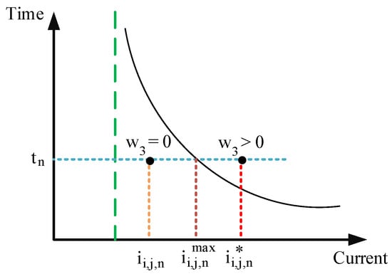
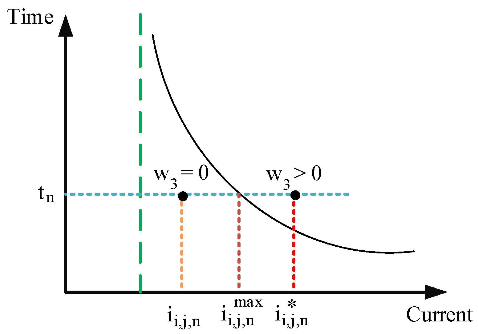
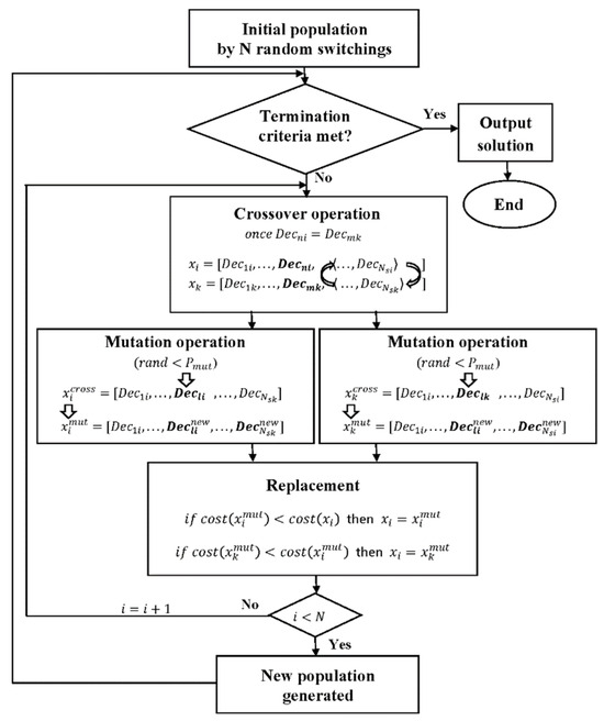
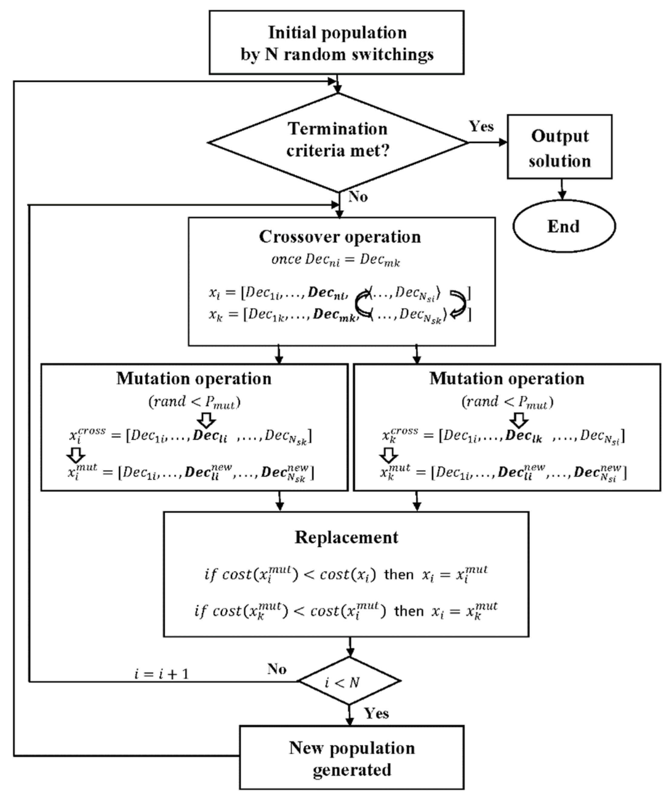
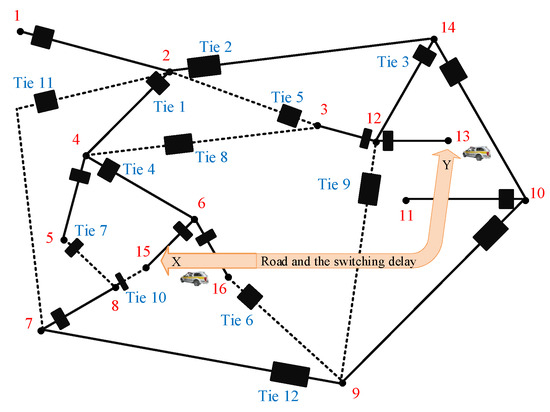
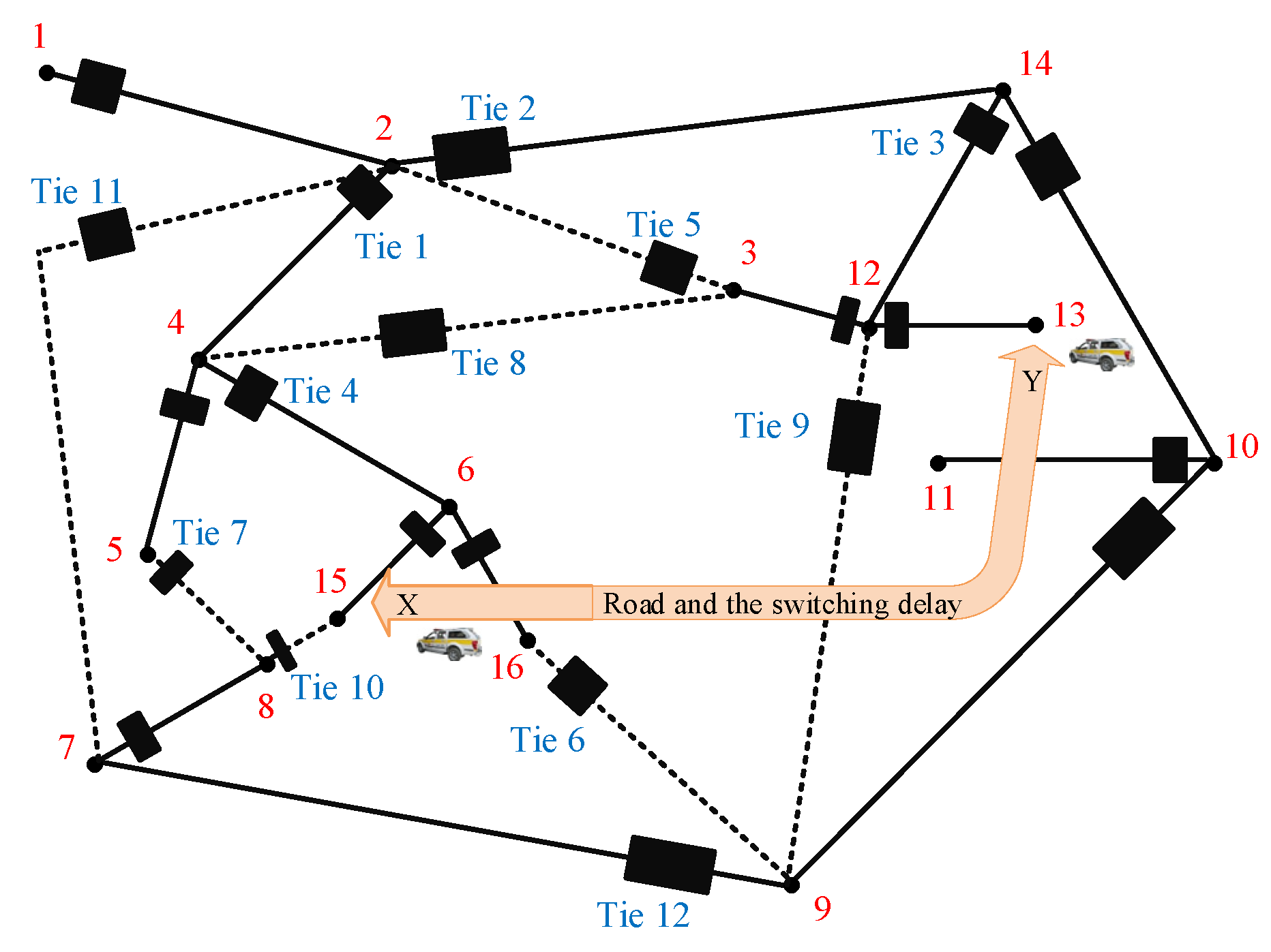
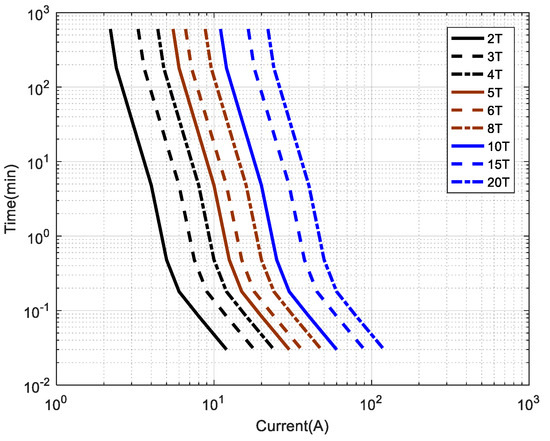
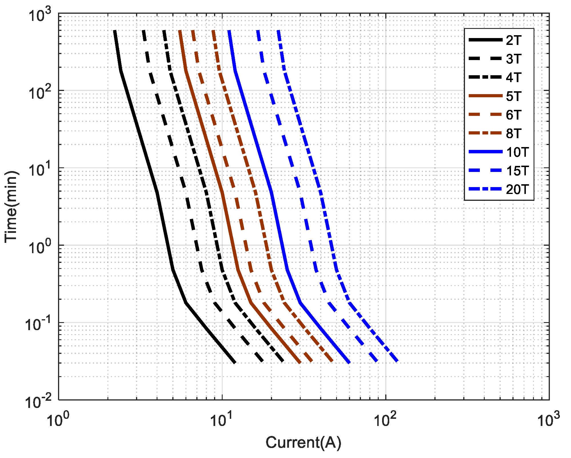
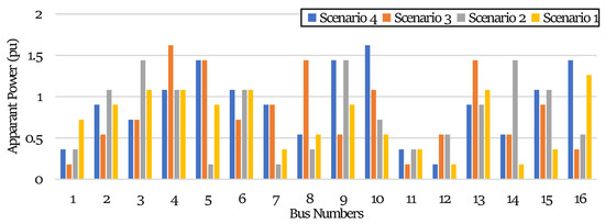
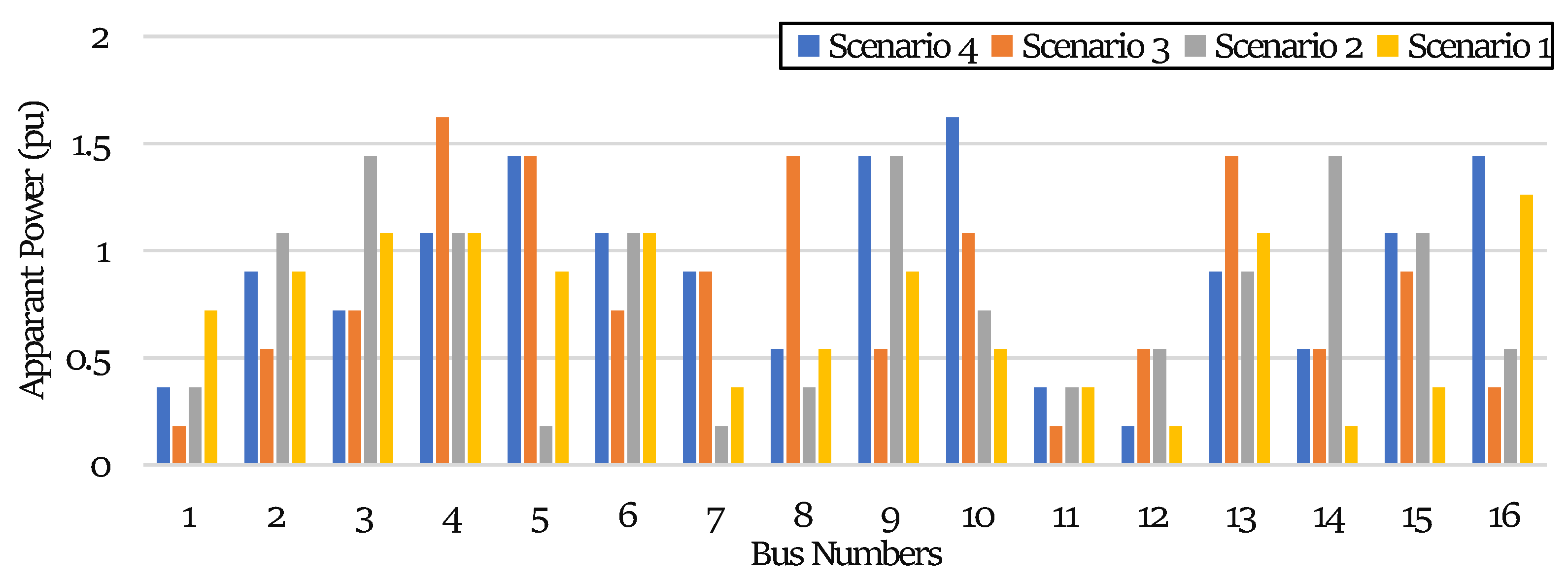
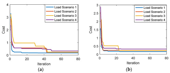
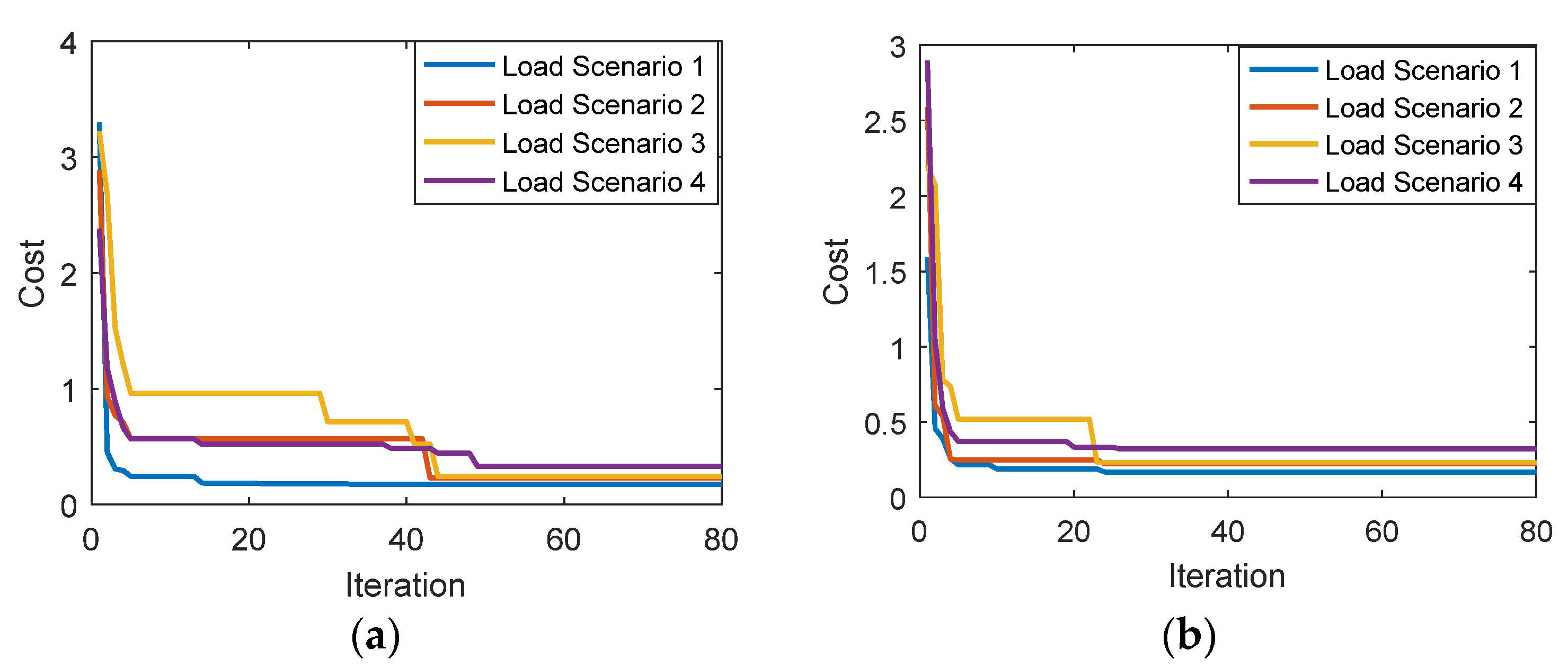
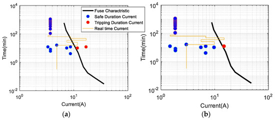
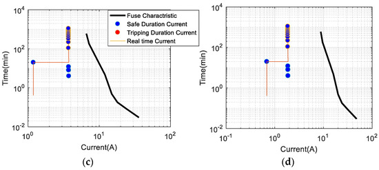
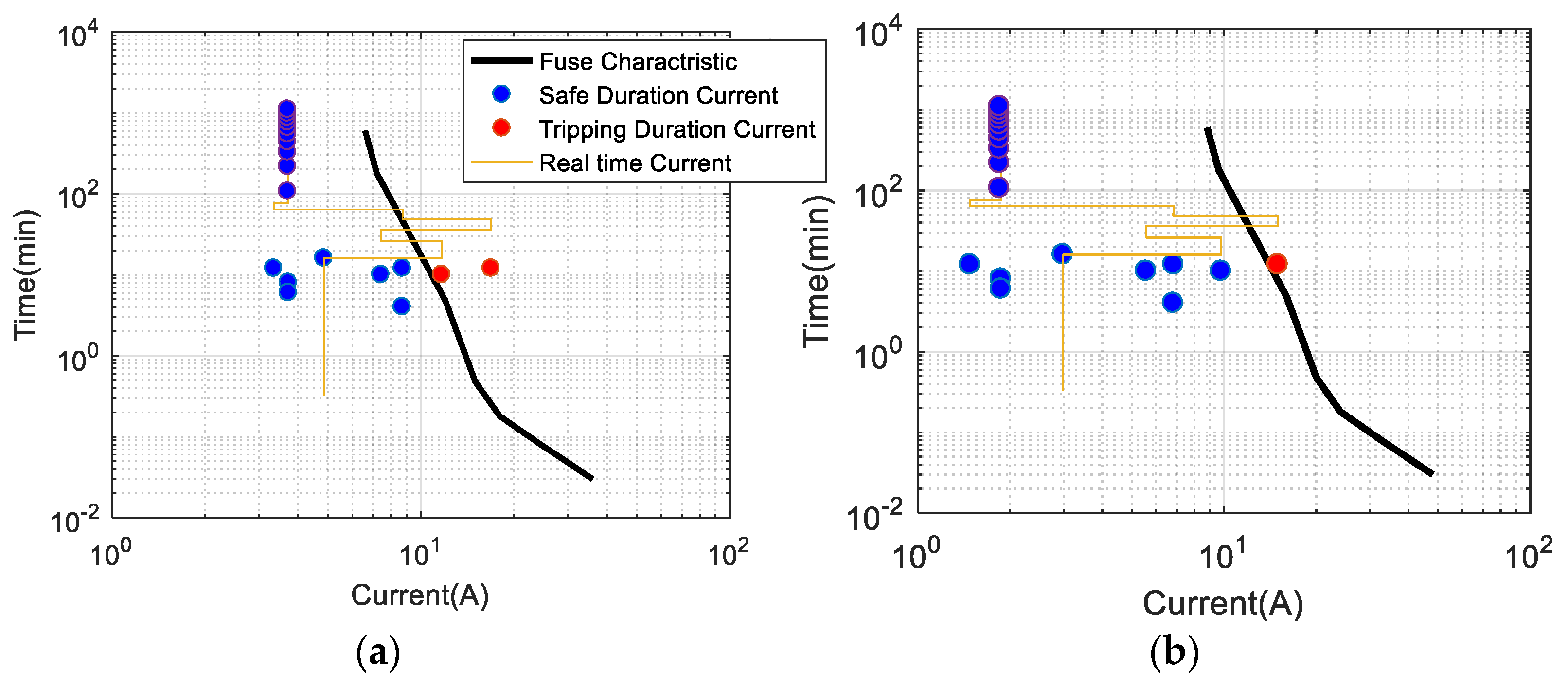
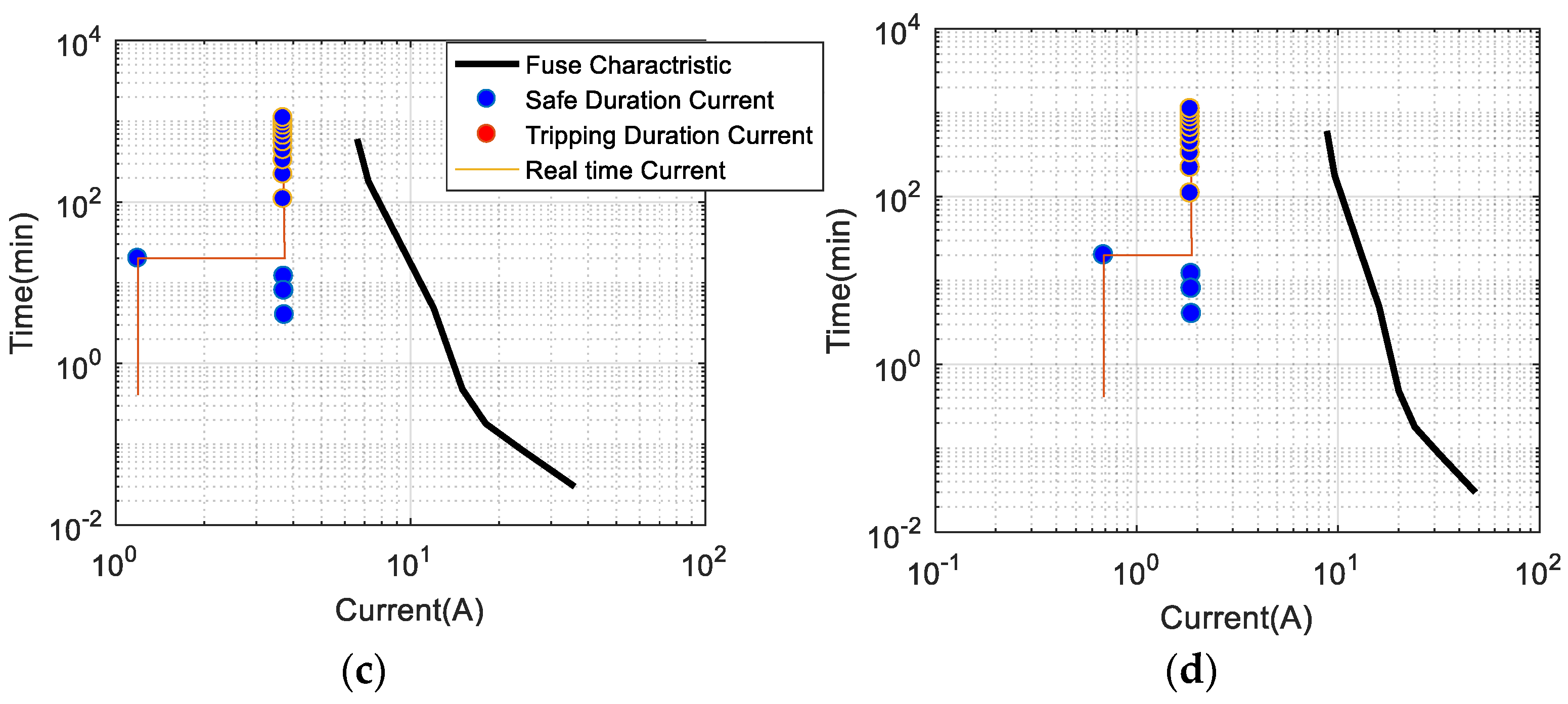
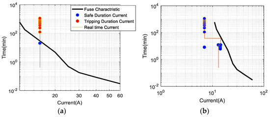
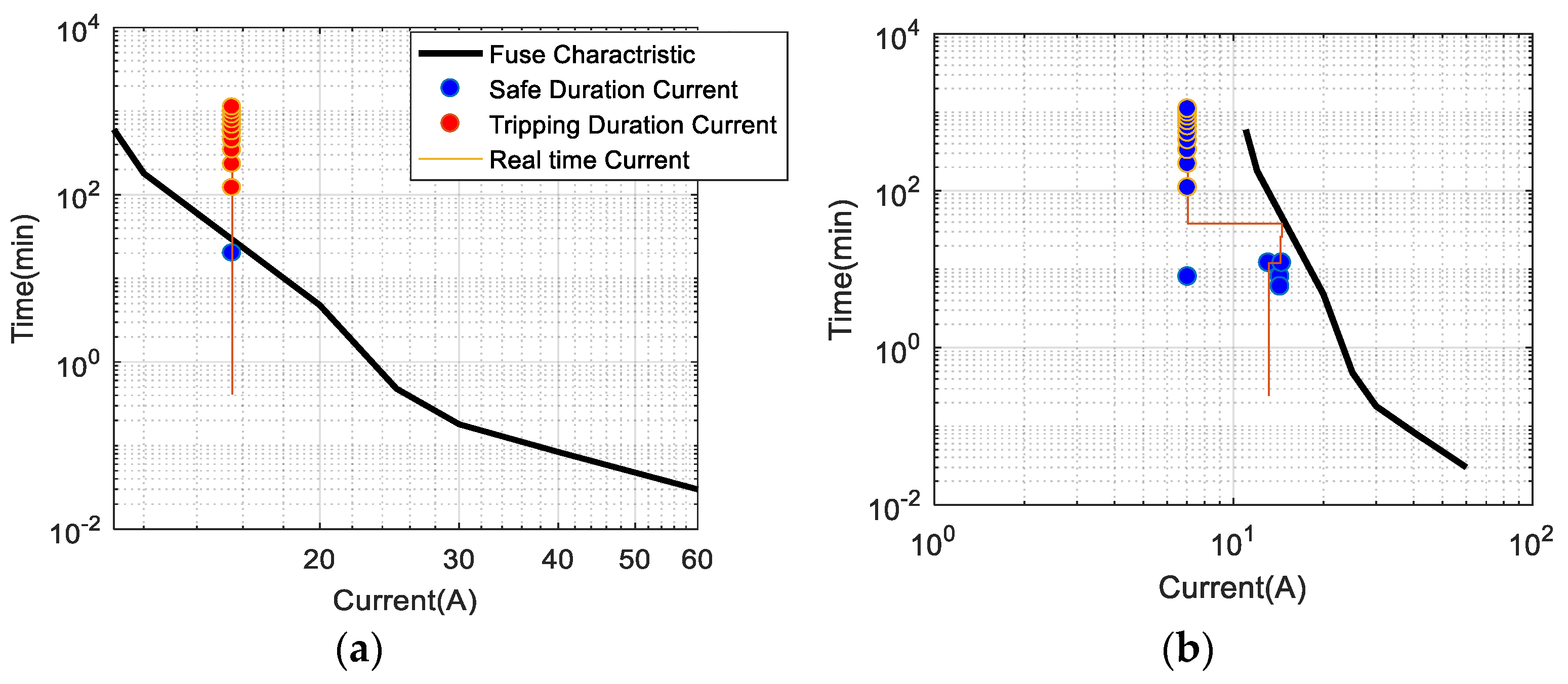
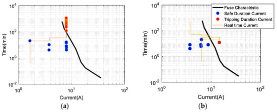
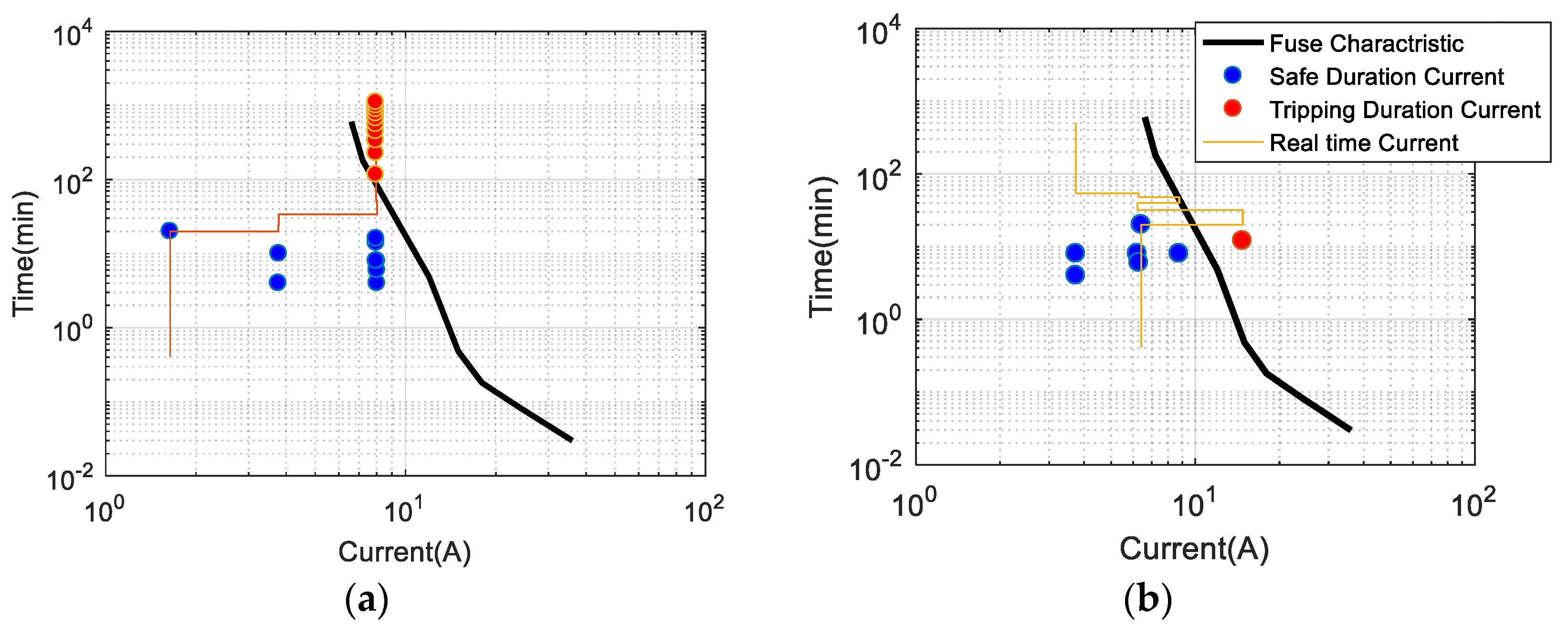
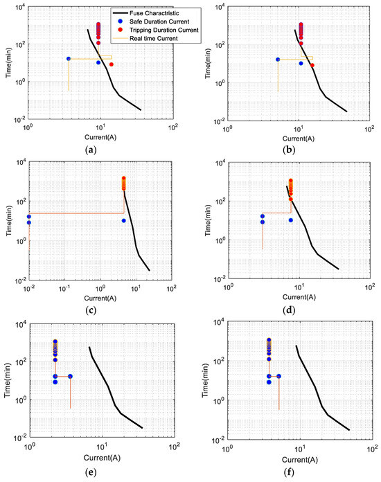
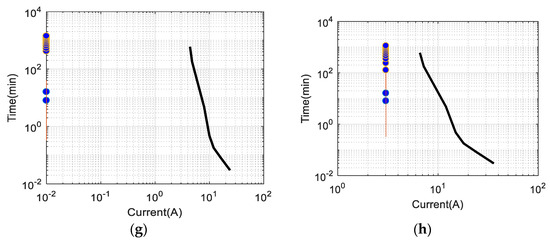
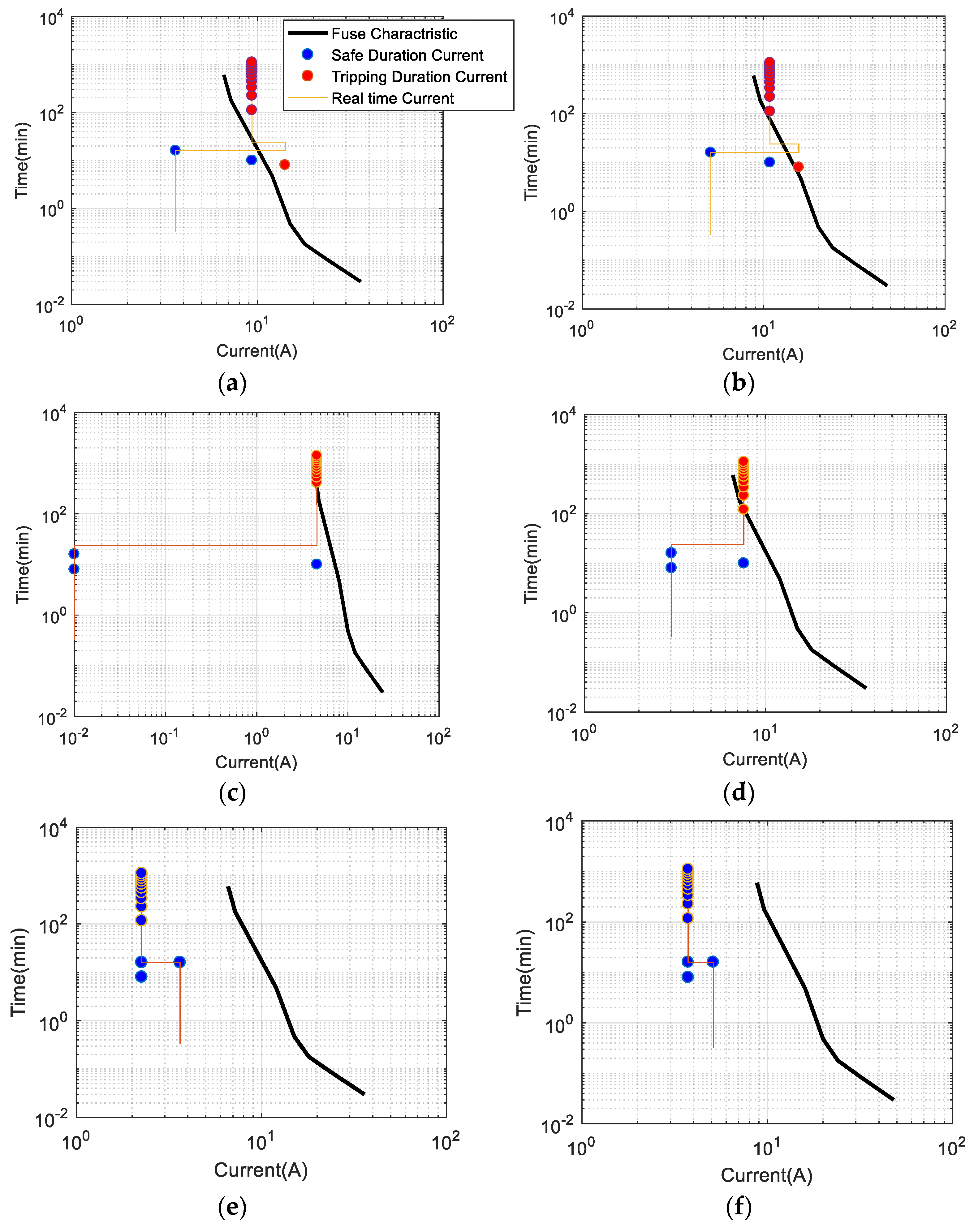
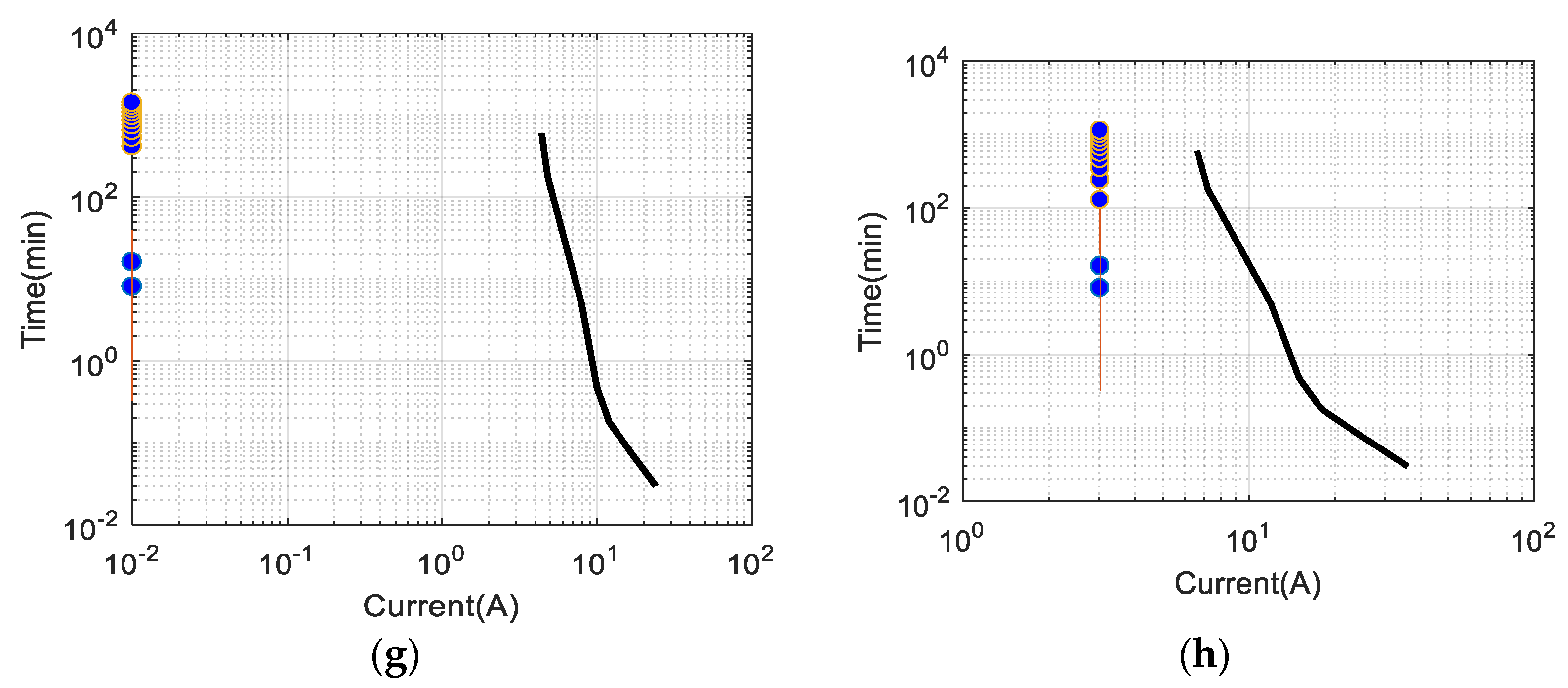
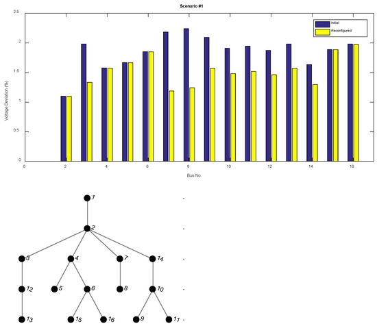
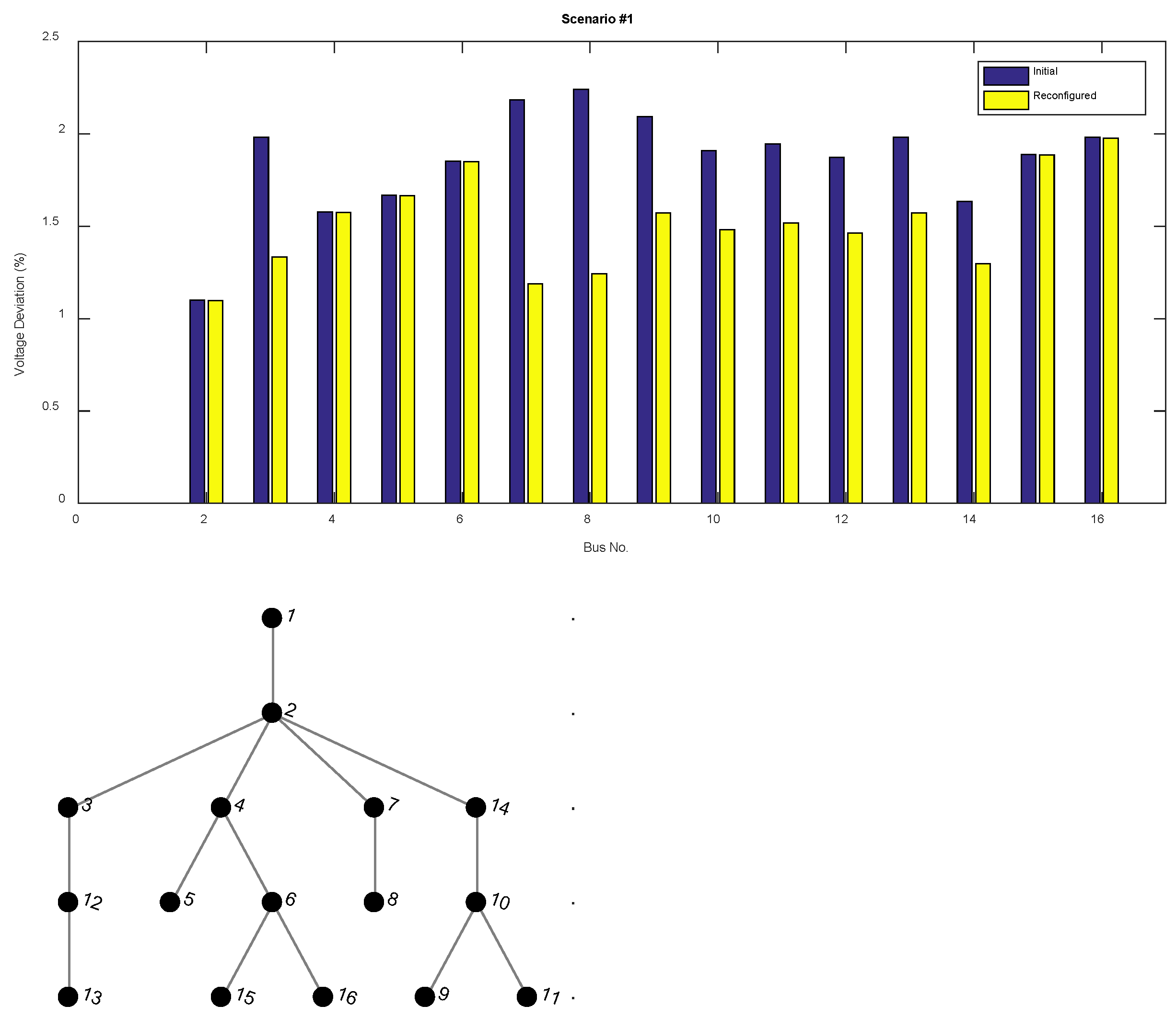
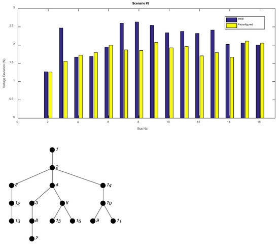
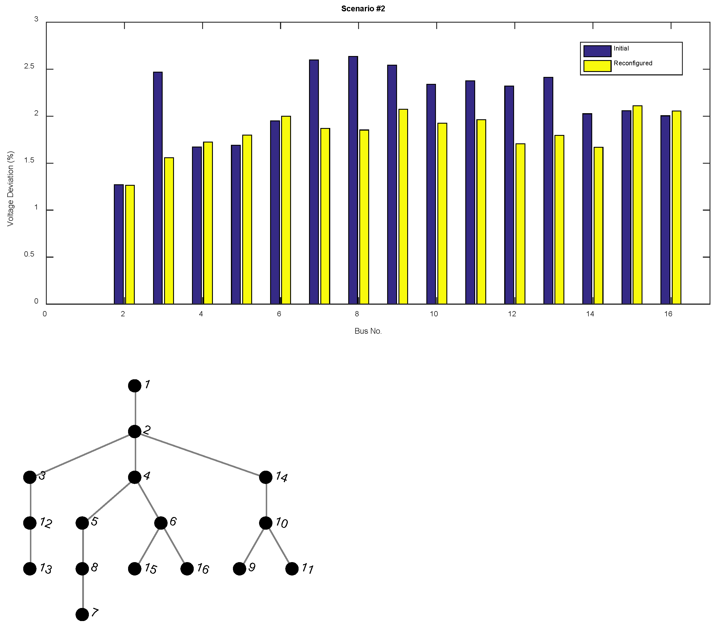
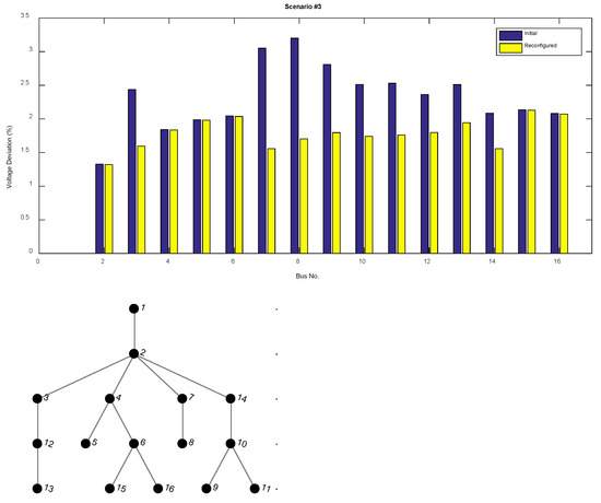
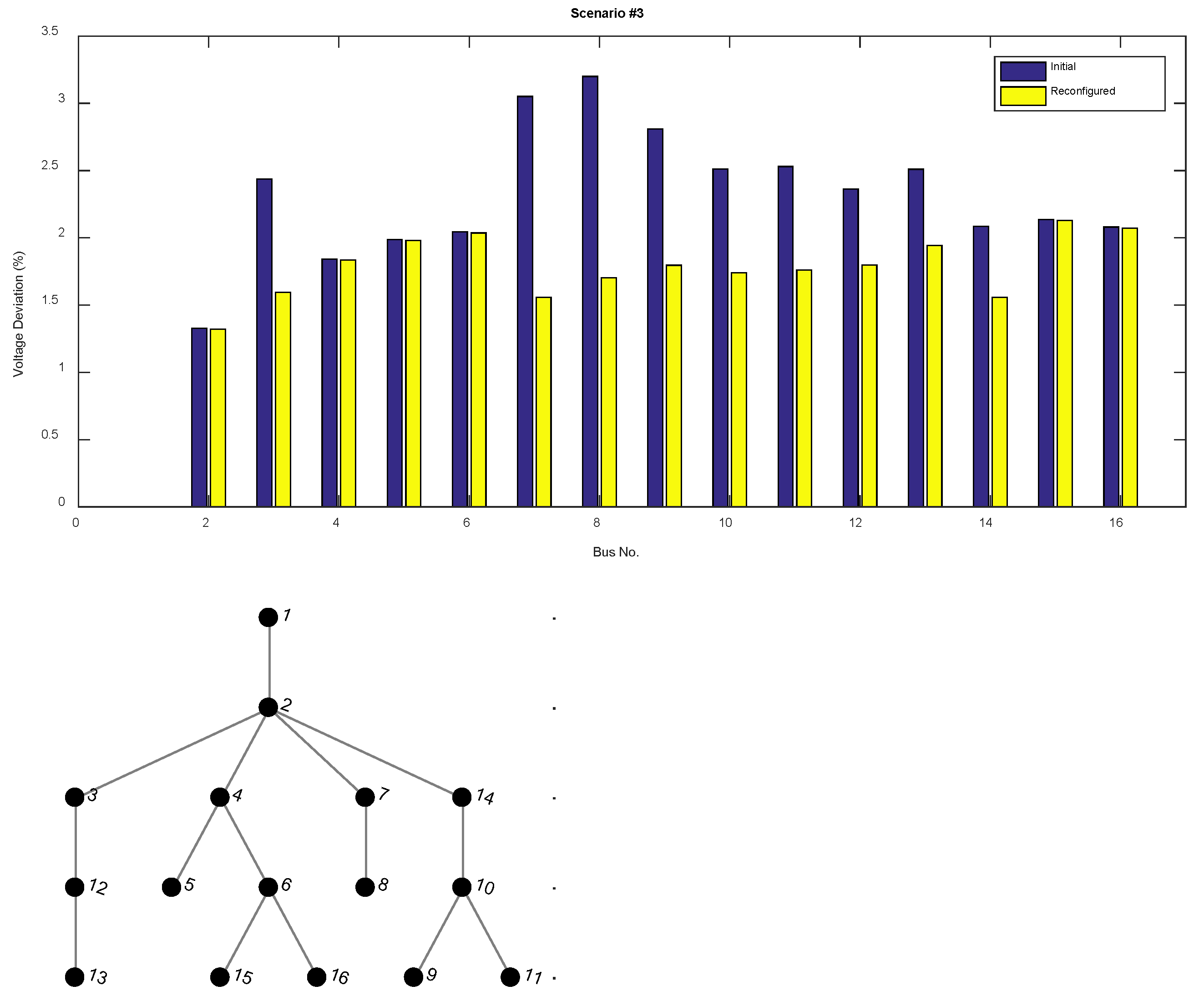
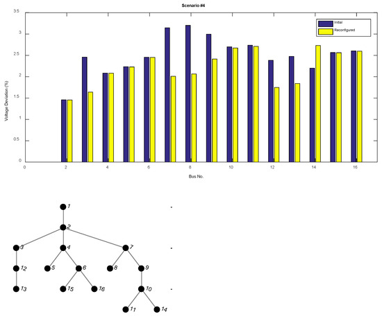
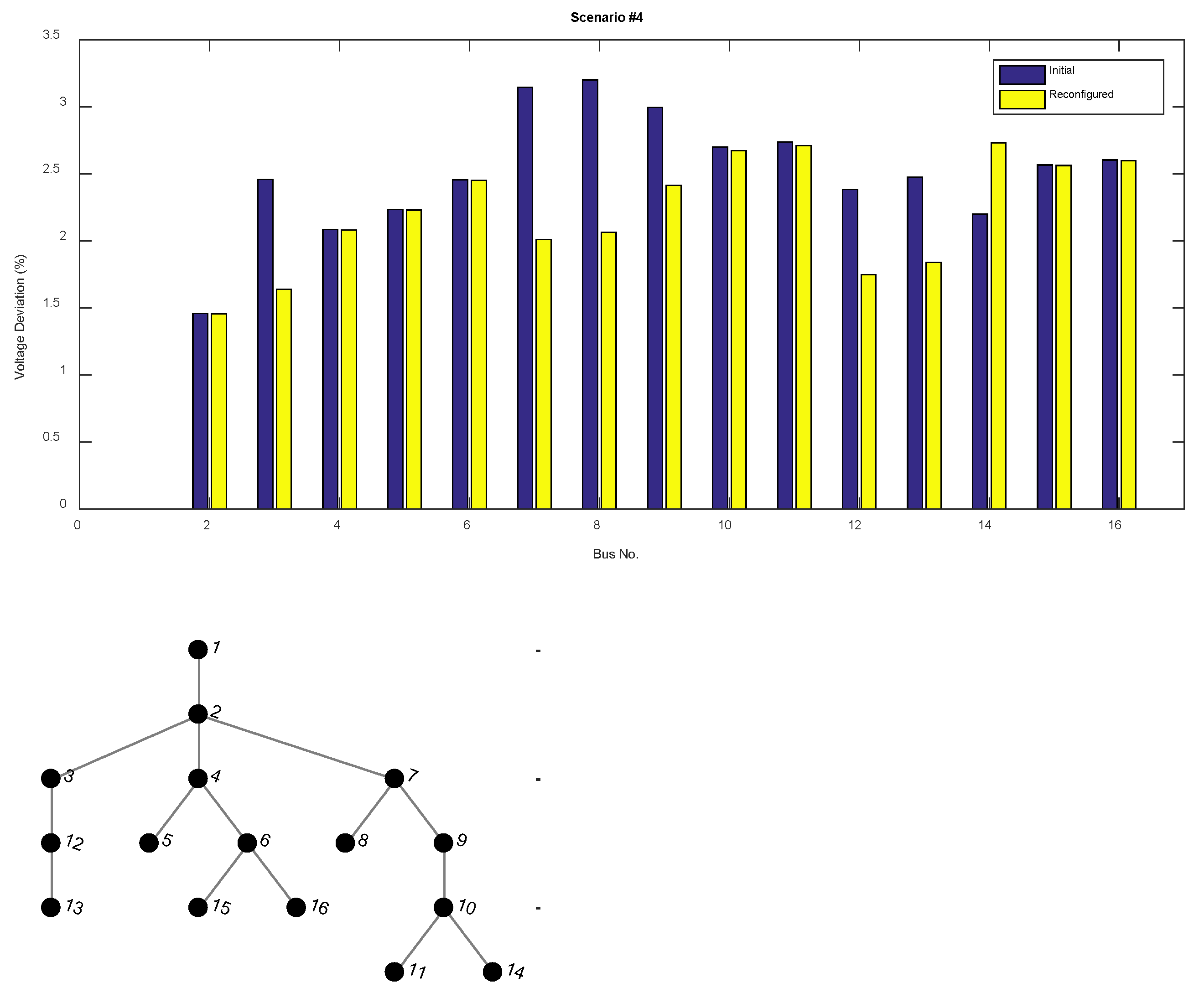
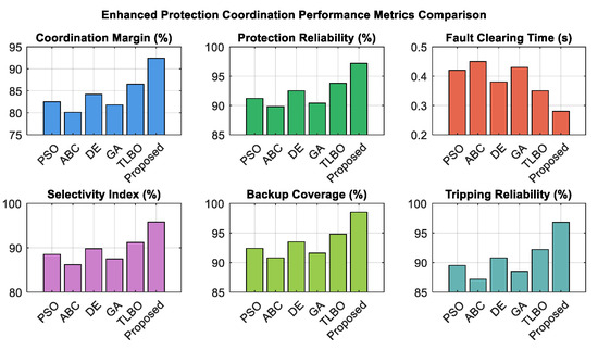
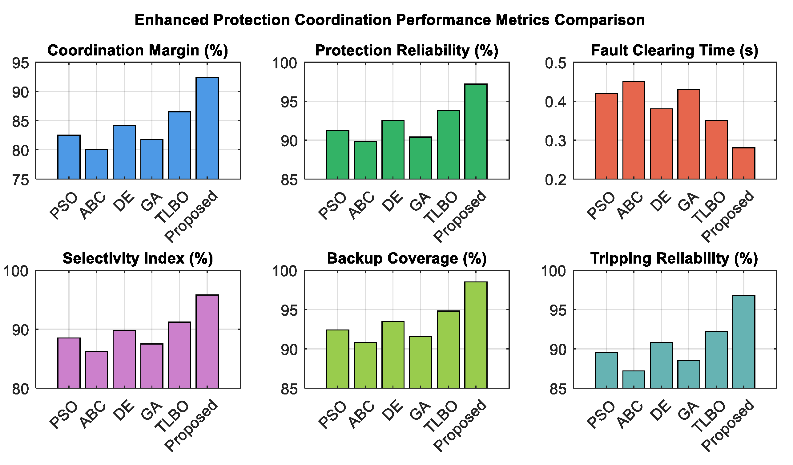
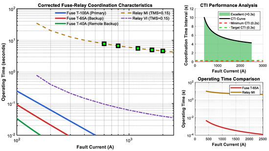
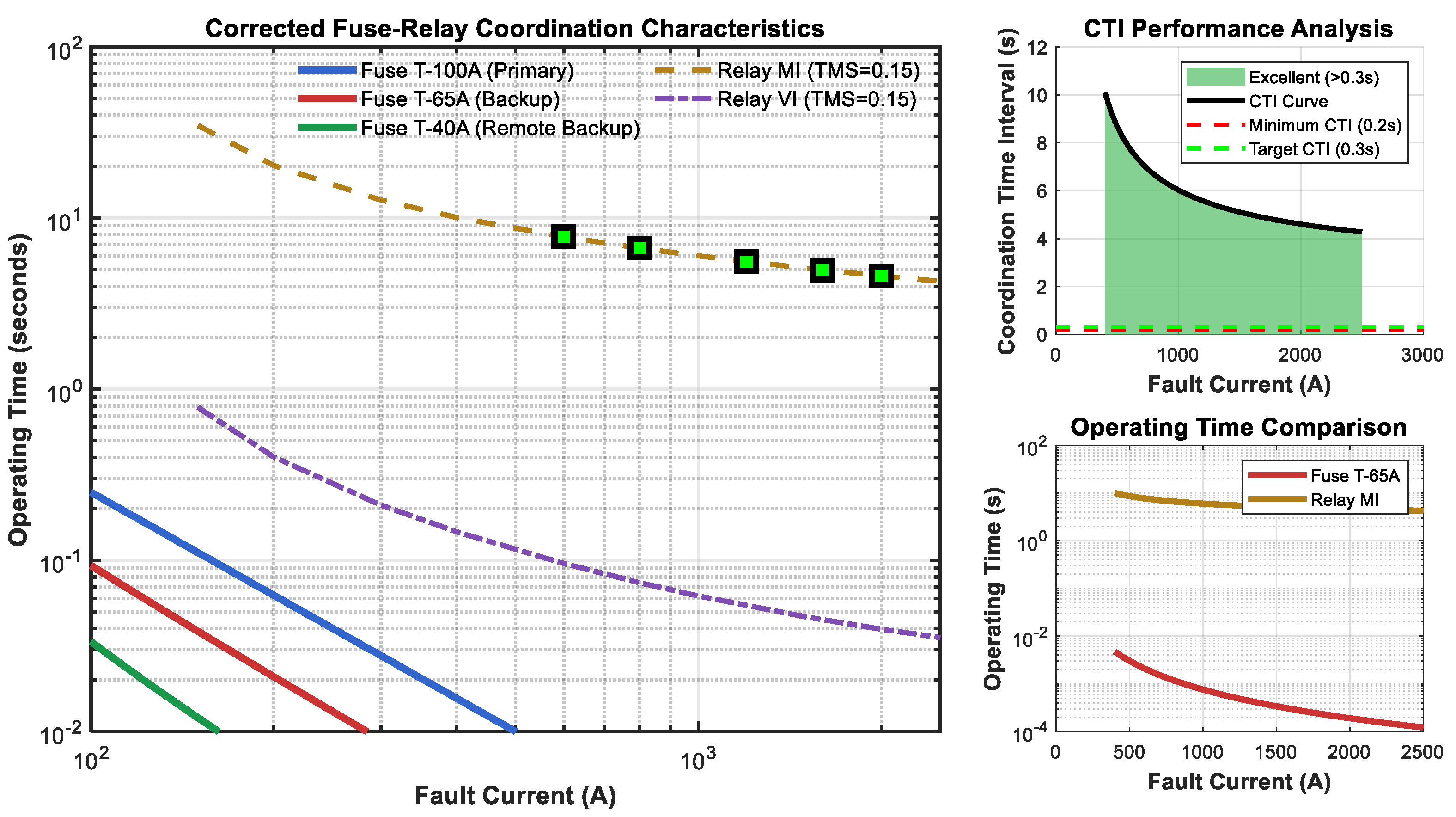
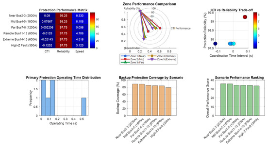
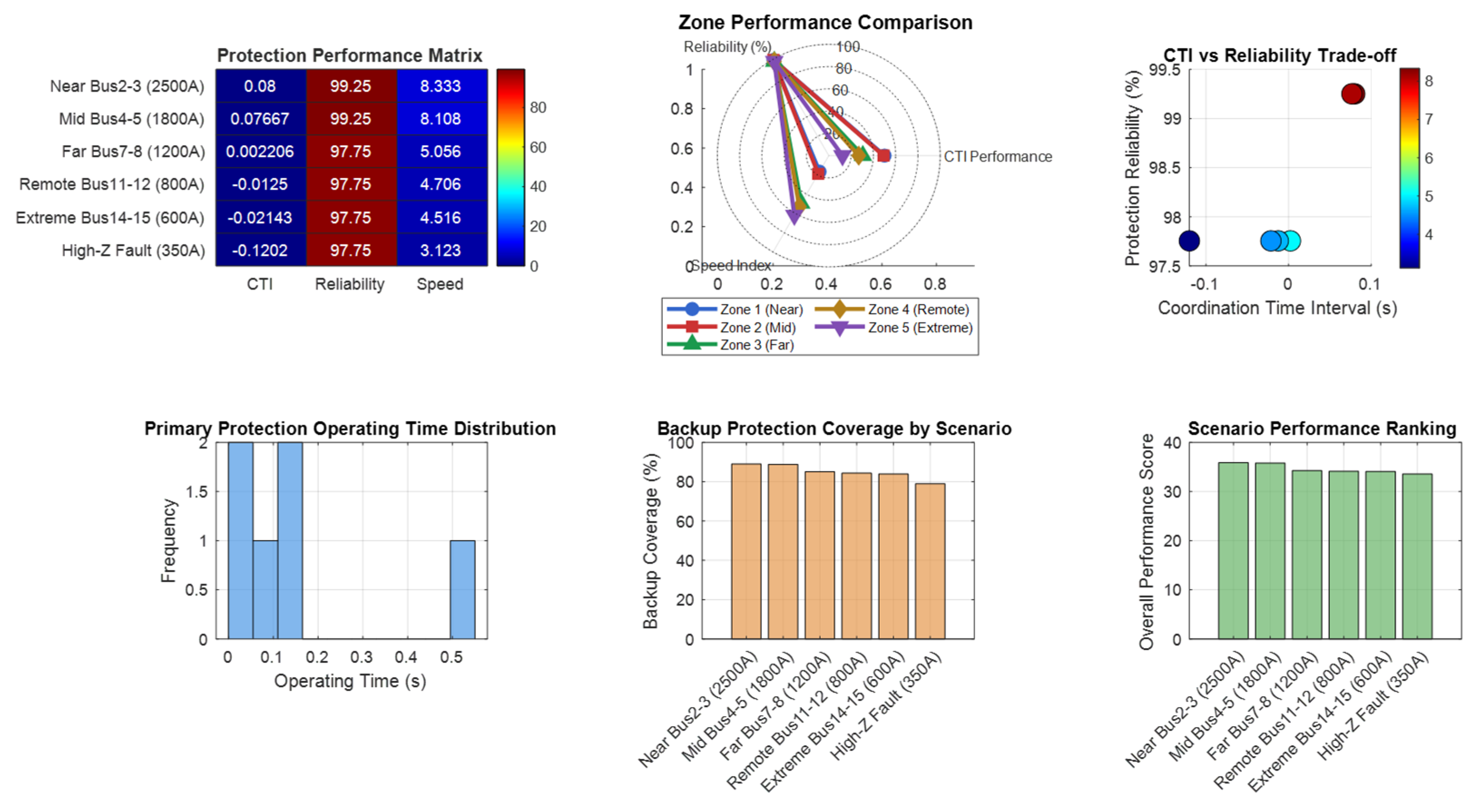
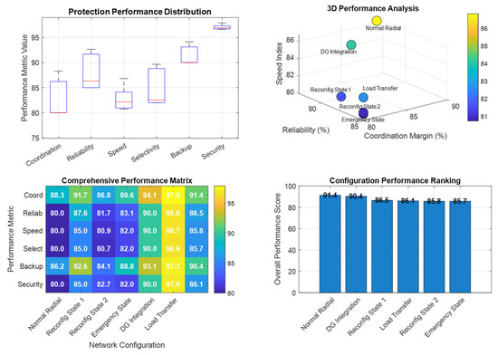
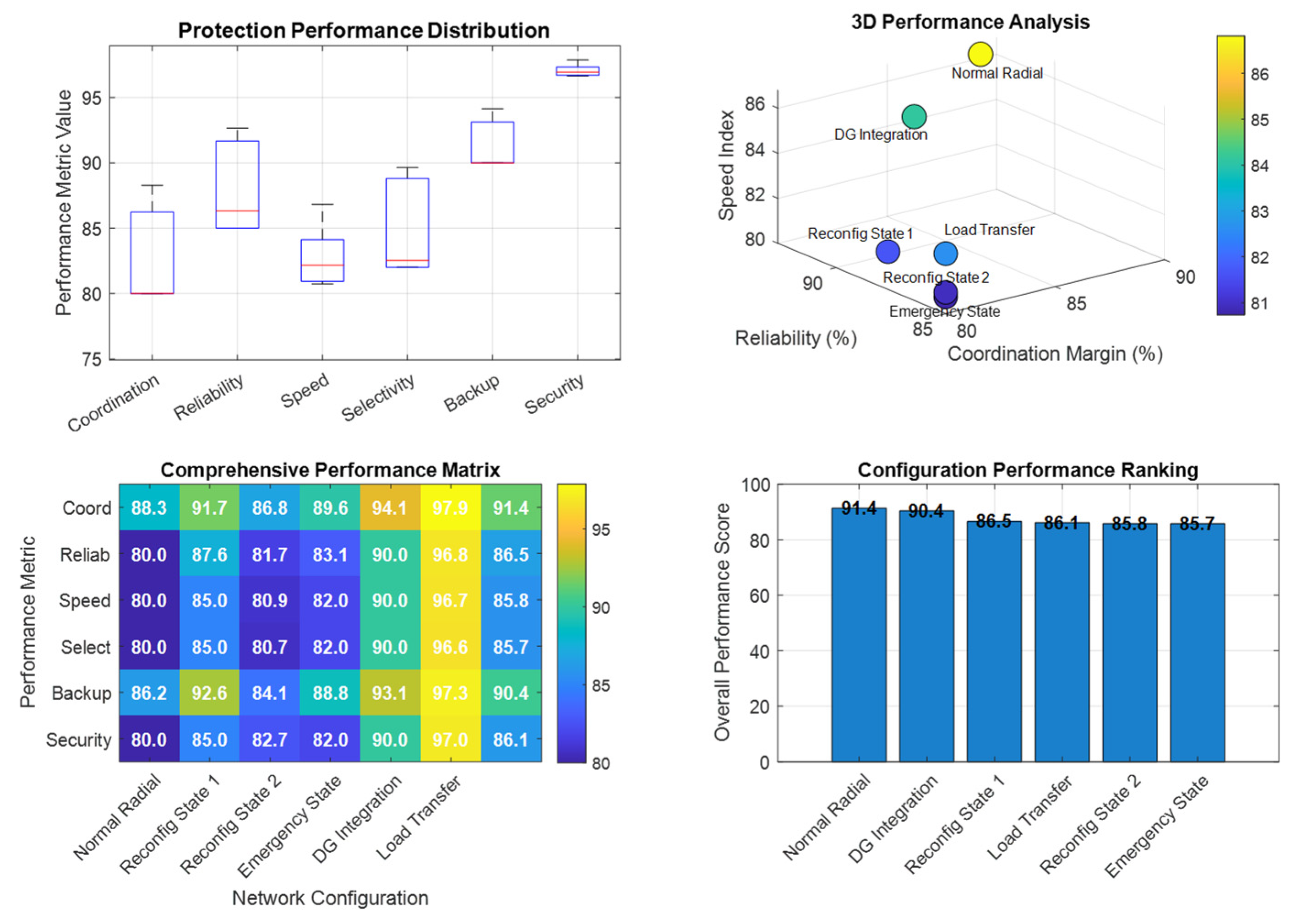

Disclaimer/Publisher’s Note: The statements, opinions and data contained in all publications are solely those of the individual author(s) and contributor(s) and not of MDPI and/or the editor(s). MDPI and/or the editor(s) disclaim responsibility for any injury to people or property resulting from any ideas, methods, instructions or products referred to in the content. |
© 2026 by the authors. Licensee MDPI, Basel, Switzerland. This article is an open access article distributed under the terms and conditions of the Creative Commons Attribution (CC BY) license.