Analysis of Fuel Economy Due to Rolling Resistance on Class 8 Tractor-Trailer Vehicles Using a Modeling Approach

Abstract

This paper investigates the influence of rolling resistance on fuel consumption in Class 8 heavy-duty vehicles, with a focus on a modeling approach through variations in the rolling resistance coefficient ($C_{rr}$) across different driving scenarios. Leveraging TruckSim’s multibody modeling approach for vehicle dynamics and MATLAB/Simulink co-simulation capability, the study provides insights into how tire rolling resistance affects energy efficiency under varying conditions while enabling controlled, repeatable comparisons across various scenarios. Results show that across the evaluated scenarios, increases in $C_{rr}$ impact the vehicle’s speed, fuel consumption, engine torque, and crankshaft spin. Specifically, increasing $C_{rr}$ from 0.004 to 0.013 was found to lead up to 68% higher fuel consumption in high demand scenarios. These findings aim to guide efforts to optimize tire design and vehicle performance that help achieve improved fuel efficiency.

1. Introduction

Heavy-duty vehicles (HDVs) are widely utilized throughout the world for goods transport, and due to this, they accounted for 20% of greenhouse gas emissions (GHG) of the EU transport sector, with the whole transport sector making up for 28.9% of all EU-27 GHG emissions [1]. In the US, the transportation sector contributed to 28.5% of the U.S. greenhouse gas emissions in 2022, with medium- and heavy-duty vehicles accounting for 22.9 percent of the sector’s emissions [2]. The high usage of HDV combined with their impact on the environment has also led to new regulations, such as the Implementing Regulation (EU) 2022/1362, for the assessment of CO² and energy consumption using the VECTO software (https://climate.ec.europa.eu/eu-action/transport-decarbonisation/road-transport/vehicle-energy-consumption-calculation-tool-vecto_en, accessed on 5 March 2026), which considers various properties such as mass, aerodynamics, and rolling resistance to certify vehicle performance [3]. This makes it necessary to investigate ways to increase their efficiency and reduce their carbon footprint. An example of this is the Super Truck Program, a Recovery Act-funded project by the U.S. Department of Energy carried out from 2010 until 2015, focused on improving the freight efficiency of Class 8 trucks [4]. The project aimed to achieve a 50% increase in vehicle freight efficiency and a 50% engine brake thermal efficiency. This was done through the development and testing of a SuperTruck Final Demonstrator vehicle, which implemented numerous advanced technologies like full tractor aerodynamics, an improved engine, a hybrid system, and the use of lightweight materials, among others. Nowadays, this project provides insights into the effectiveness and commercial viability of a wide range of advanced technologies and demonstrates the potential for substantial improvements in fuel consumption in heavy-duty trucks, such as the improvement in tire technologies that Michelin constantly strives to reach.

The rolling resistance of tires is one of the key contributors to fuel consumption in vehicles, and a state-of-the-art review mentions that it can be responsible for up to 30% of a vehicle’s fuel consumption [5], and how, aside from the tire design, the tire’s operational parameters like normal load and rolling speed have a significant impact on rolling resistance. A literature review on the relationship between operational parameters and rolling resistance concludes that a higher temperature leads to a decrease in rolling resistance, that the combination of pavement and tire does not always lead to a change in $C_{rr}$, and that speed and torque (driving or braking) generally increase rolling resistance [6]. A study evaluated the impact of various operating parameters on braking friction and rolling resistance on asphalt surfaces through simulations and experimental tests, and found that tire load was found to have a higher influence on rolling resistance than braking friction, becoming more critical at speeds above 80 km/h [7]. Similarly, the results from experiments in different road surfaces show that an increase in tire load (for a given tire, road pavement, and speed) always leads to an increase in rolling resistance force at constant inflation pressure, the same cannot be said about the rolling resistance coefficient, which is specific to the combination of tire and pavement, and therefore $C_{rr}$ may decrease, increase, or stay fairly constant [8]. The impact of operating factors has also been studied for passenger electric vehicles, where [9] identified that decreasing the ambient temperature from 30 °C to 0 °C can increase rolling resistance 57.5%, and that increasing the vehicle’s mass from 2000 to 2300 kg leads to 15.7% rise in rolling resistance.

The influence of tire rolling resistance on fuel consumption has been analyzed using $C_{rr}$ measurements from different modern passenger car tires on different road pavements, concluding that fuel consumption can be decreased by up to 20% with the combination of electric vehicle tires and low rolling resistance road pavements [10]. For heavy-goods vehicles, in-service operation data collection is carried out to analyze the benefits of low-rolling-resistance tires on fuel consumption [11], with the study concluding that these tires can save up to 8.37% of fuel in typical driving conditions on UK motorways. In another study, the tire and pavement interaction model proposed by [12] shows that energy consumption due to rolling can increase by 68.3% with increased tire load, and that tire pressure can reduce energy consumption by 20.45%. Focusing on Class 8 tractor-trailers, a study on the impact of tire temperature and inflation pressure on fuel consumption was carried out using sensors installed on a real vehicle, and the conclusion was that inflation pressure had a very minor and barely measurable effect on fuel consumption [13]. Additionally, another study measured the rolling resistance and aerodynamic resistance forces for different combinations of trucks and trailers and different tire types, and found that a 2 bar decrease in tire pressure could increase the rolling resistance coefficient by 11% on average [14].

To help reduce vehicle fuel consumption and, in turn, reduce costs and greenhouse emissions, it is necessary to understand the forces a vehicle needs to overcome to be able to move, and as discussed in [15], tire rolling resistance can account in average 20% of a vehicle’s resistance to movement, and a tire with a rolling resistance coefficient of 12 kg/t, can account for up to 30% of a vehicle’s fuel consumption. With these considerations in mind, it becomes of utmost importance to develop and use tires with lower rolling resistance. This paper investigates the influence of rolling resistance on fuel consumption in Class 8 heavy-duty vehicles using a modeling-based approach that examines variations in the rolling resistance coefficient ($C_{rr}$) in different driving scenarios. In this work, the simulated $C_{rr}$ values are intended to represent differences in tire technology and design such as the materials and construction, rather than changes in road and operating conditions alone. The objective is to analyze how rolling resistance affects energy efficiency across varying driving conditions using the well-established TruckSim software (https://www.carsim.com/products/trucksim/, accessed on 5 March 2026) adopted by the Automotive Industry. The findings aim to guide efforts to optimize tire design and vehicle performance that help to achieve improved fuel efficiency.

The outline content of this paper is as follows. In the next section, the methodology for the simulation-based analysis of fuel consumption considered in this paper is presented. Then, Section 3 describes in detail the simulation configuration in the TruckSim software for tractor-trailer specifications, tire modifications, and the driving cycles considered. The simulation results are then analyzed and discussed in Section 4, and Section 5 provides some conclusions and observations from the work carried out.

2. Methodology

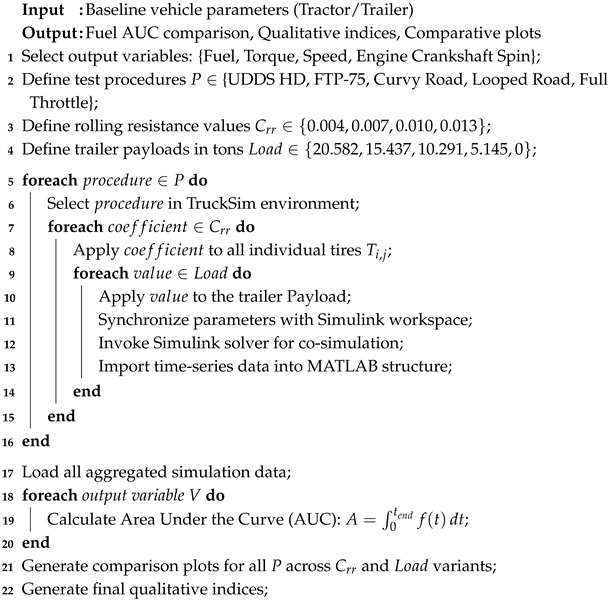
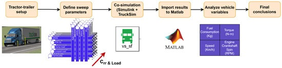
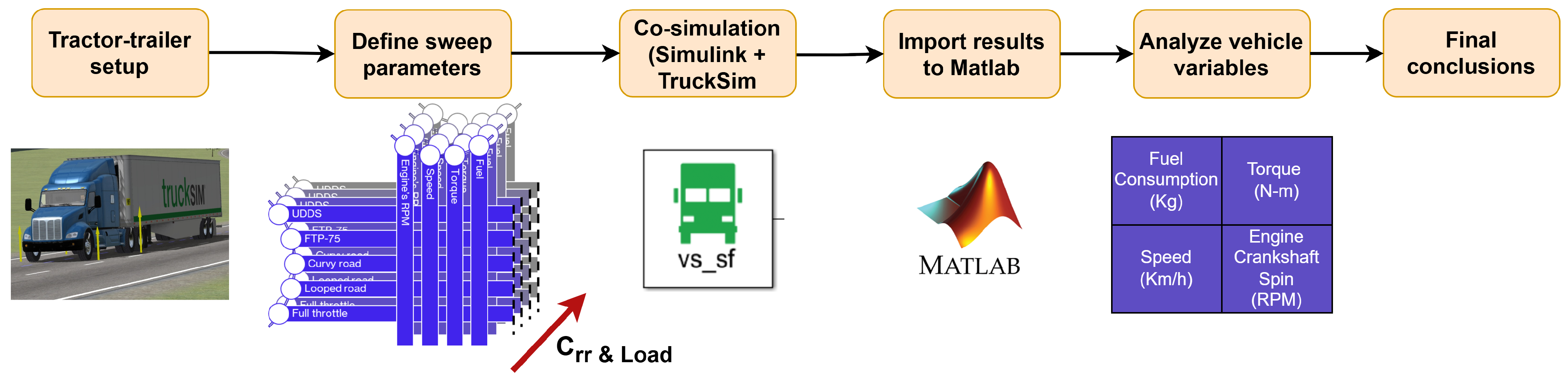
Figure 1 illustrates the general methodology used to analyze the rolling resistance coefficient on fuel consumption in the simulation environment based on the TruckSim software. Firstly, the truck and general setup parameters are defined in the simulation; the simulation must be able to run in MATLAB (R2025a)/Simulink (25.1), where the output variables are saved as matrices and imported into the MATLAB workspace for further processing. These data can be used to graph and analyze the differences between the various tests, with a focus on variations in the rolling resistance coefficient used in TruckSim’s tire model. This approach allows for a comprehensive comparison of fuel consumption across different driving scenarios and rolling resistance values. Algorithm 1 covers in detail the routine carried out for the simulation, where the most important variables have been defined according to the state-of-the-art review, which includes fuel consumption, the engine’s torque, and crankshaft spin (RPM), and the vehicle’s speed.

Figure 1. Methodology to analyze the $C_{rr}$ impact on the fuel consumption under different driving scenarios.

In addition, four different rolling resistance coefficients ($C_{rr}$) were selected for the tire model to evaluate their effect on fuel consumption. For driving scenarios, five distinct and classical test procedures were selected for analysis: UDDS HD, FTP-75, Curvy Road, Looped Road with Banking and Full Throttle Acceleration with 6% grade. The first two are standard drive cycles, and the rest are TruckSim-specific scenarios. Finally, to further analyze fuel consumption, different trailer loads given in tons were simulated, ranging from a full load to an empty trailer. With all necessary variables defined, a parameter sweep was performed using co-simulation of TruckSim and Simulink, with the resulting data imported and analyzed in MATLAB.

As depicted in the methodology diagram illustrated in Figure 1 and the Algorithm 1, the Software-in-the-Loop environment between TruckSim and MATLAB ensured a comprehensive comparison of fuel consumption under diverse driving conditions, rolling resistance coefficients, and trailer loads, using the combined capabilities of both software. In the end, the impact of the rolling resistance coefficient is analyzed to determine, from a global perspective, the effect of tire technology (rolling resistance) on tractor-trailer performance and its impact on energy consumption.

Algorithm 1: TruckSim tire Crr analysis and data processing routine

3. Simulation Setup

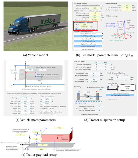
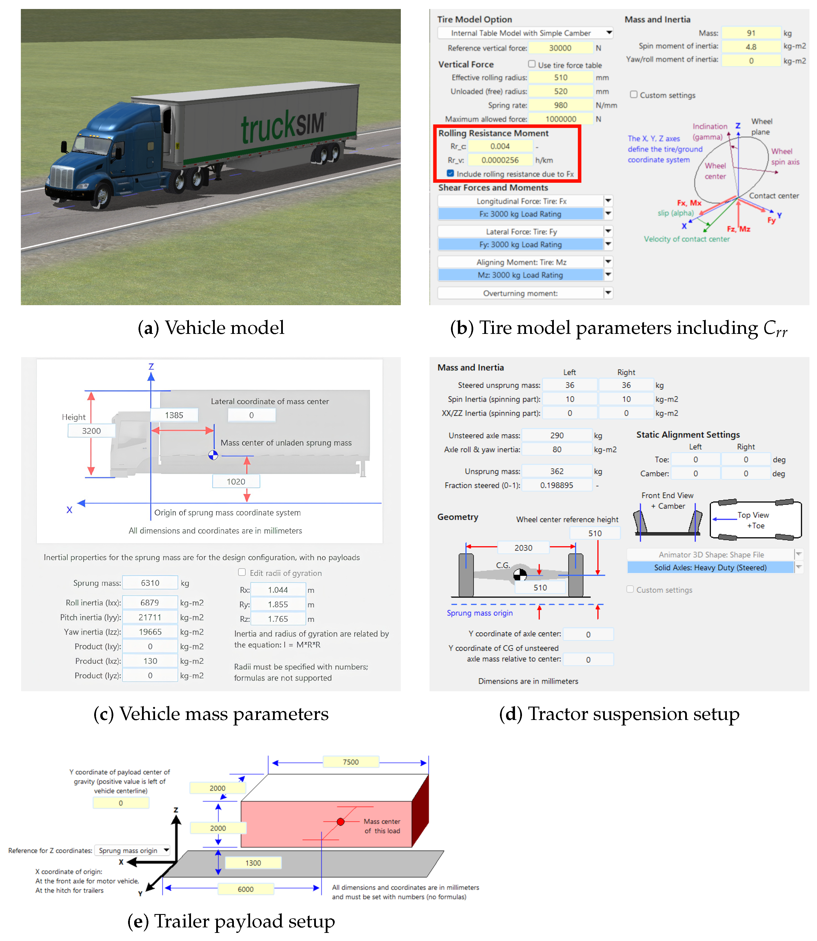
For the simulated test vehicle, a three-axle sleeper-cabin tractor paired with a two-axle van trailer preset in TruckSim was used as the base platform to evaluate the impact of rolling resistance on fuel consumption. Figure 2 illustrates some of the main components used to model the longitudinal vehicle dynamics in TruckSim.

Figure 2. TruckSim vehicle model parameters used for the three-axle sleeper cabin tractor paired with a two-axle van trailer.

This vehicle configuration, shown in Figure 2a, uses nominal TruckSim parameters that are meant to be representative of a typical Class 8 tractor-trailer. The three-axle tractor features a 330 kW diesel engine with a maximum torque of 1894 Nm and an 18-speed manual transmission. The trailer has a payload capacity of 20.582 tons and was equipped with an air suspension, providing a realistic representation of a typical heavy-duty transport configuration.

TruckSim uses a system-level modeling approach that allows the analysis of complete vehicle dynamics and components in varied and detailed simulated driving conditions. This approach allows the software to model the vehicle’s geometry, masses, aerodynamics, and inertial properties, but also the suspension, steering characteristics, powertrain, braking behavior, and tire and road interactions. The vehicle model in particular is based on parameters of the vehicle size, sprung and unsprung mass shown in Figure 2c,d, where the center of gravity is also defined in relation to the sprung mass coordinate system origin. For the vehicle’s weight distribution, TruckSim utilizes a multibody dynamics approach in which these masses are accounted for in conjunction with payloads, such as the one used for the trailer (see Figure 2e), which are treated as bodies with mass and inertia rigidly attached to the vehicle’s sprung mass. In the case of the tractor-trailer modeled in this work, the weight distribution is further influenced by the hitch connections, which transfer vertical forces between the tractor and the trailer.

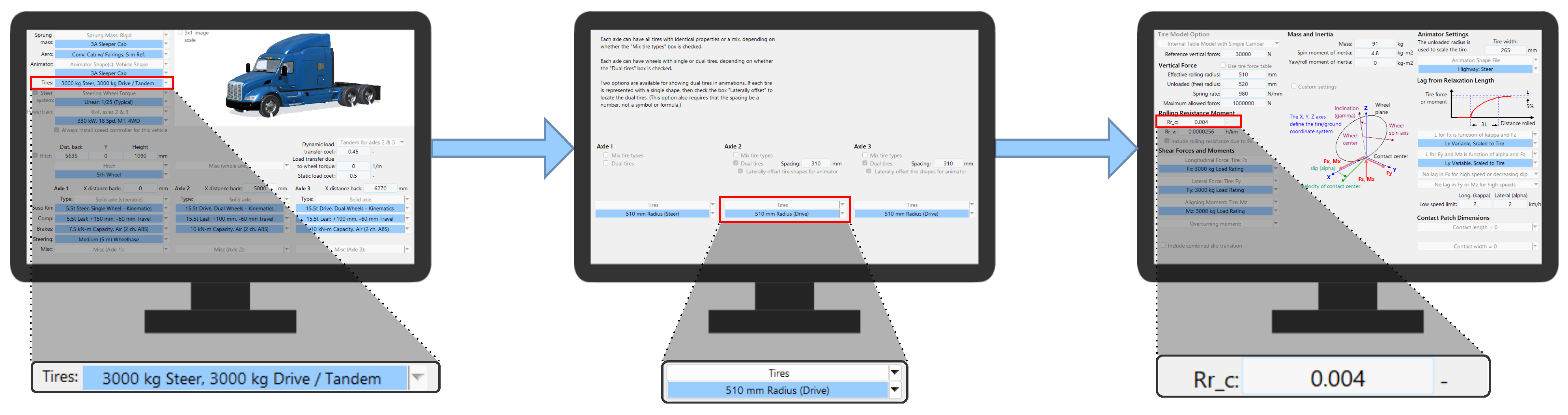
Figure 2b shows the tire’s parameters of TruckSim’s Internal Table Model with Simple Camber used in this work. This model considers tire dimensions, as well as shear forces and moments as functions of load, longitudinal and lateral slip, angle, and friction between the tire and the surface, just as they would be measured in a laboratory. This is combined with calculations of other forces and moments not included in those tables using the works of [16,17]. Figure 3 illustrates the process for modifying the $C_{rr}$ of each individual tire, beginning with the vehicle model screen, where tires are one of the various components considered in the multibody dynamics vehicle model. Selecting the tires shows the current tire option for each axle of the vehicle, and in dual-axle configurations, it shows the combination of different tire options. Finally, the last screen includes all the parameters of the tire model that have been discussed previously. For this work, each individual tire model was modified to use the same $C_{rr}$ value in each simulation run.

Figure 3. Tire $C_{rr}$ selection procedure for each tire on the tractor-trailer model.

The four $C_{rr}$ values chosen for this analysis were selected based on the works carried out in [14,18], where different types of heavy-duty vehicles are analyzed to obtain their tires’ rolling resistance coefficients. Table 1 shows the $C_{rr}$ values and the types of tires and conditions they most accurately represent based on the works mentioned. In addition, the difference between the considered $C_{rr}$ values in this study surrounds the 30%, equivalent to the typical reduction of the rolling resistance coefficient of a wasted tire in a truck/bus after 15 years of normal usage [19]. Such that the considered $C_{rr}$ values represent those rolling resistance coefficients of different commercial tires for Heavy-Good Vehicles, or could be interpreted as $C_{rr}$ values for tires with different tread depths.

Table 1. $C_{rr}$ values chosen in this study and their real-world interpretation.

${\mathit{C}}_{\mathit{r}\mathit{r}}$	Type of Tire	Reference
0.004	385/55R22.5 tire with an axle load of 7 ton, inflation pressure of 9.0 bar and operating temperature of 46 °C	[14]
0.007	445/45R19.5 tire with an axle load of 4 ton, inflation pressure of 8.5 bar and operating temperature of 26 °C	[14]
0.010	265/70R19.5 tire with an axle load of 7 ton, inflation pressure of 8.5 bar and operating temperature of 26 °C	[14]
0.013	Calculated for an unloaded Class 8 truck with a weight of 11,254 kg	[18]

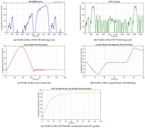
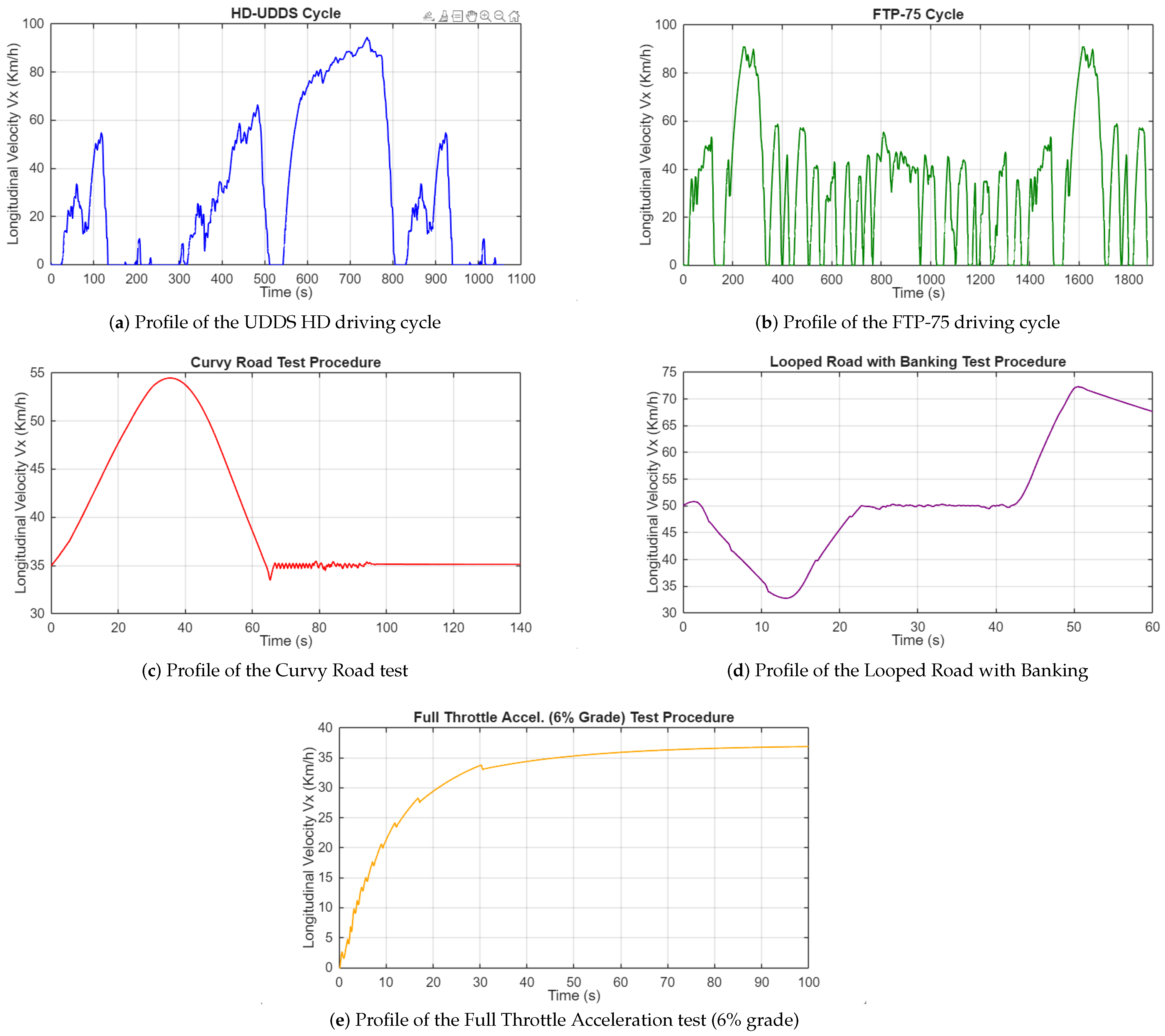
As mentioned earlier, five driving cycles have been considered in this simulation-based analysis and are described next. Starting with the Urban Dynamometer Driving Schedule for Heavy-Duty Vehicles (UDDS HD), which is a test cycle developed by the US Environmental Protection Agency (EPA). This test, as seen in Figure 4a, simulates non-freeway driving in New York (NY) and Los Angeles (LA), and freeway driving in LA. The UDDS HD test lasts 1060 s, a distance of approximately 8.9 km, a maximum speed of 93.3 km/h, and an average speed of 30.4 km/h [20].

Figure 4. Longitudinal velocity ($V_x$) in the different driving cycles considered in this simulation-based fuel consumption analysis.

On the other hand, the Federal Test Procedure (FTP)-75 is a legislative driving cycle established in the US and is used by the government to certify automobile emissions [21]. This test cycle is used to evaluate fuel economy and emissions under simulated city driving conditions. As shown in Figure 4b, the test has a duration of 1874 s and includes periods of acceleration, deceleration, and idleness, with an average speed of 33.9 km/h, a maximum speed of 90.16 km/h, and covers a distance of 17.68 km.

The Curvy Road test involves a simulated driving environment that features three turns with slight banking. The road also includes a 10-m drop in elevation, adding vertical variation to the driving path. This test scenario reaches a maximum speed of approximately 55 km/h, as can be seen in Figure 4c, and after the elevation drop, the vehicle is set to maintain a constant speed of 35 km/h. This test scenario is ideal for analyzing the impact of rolling resistance on fuel consumption under dynamic driving conditions, where the vehicle experiences continuous changes in direction, elevation, and acceleration.

The Looped Road with Banking test, shown in Figure 4d, simulates driving on a road with various twists, elevation changes, and banking. Unlike a circular track, the road layout includes a combination of curves and slopes, which require the vehicle to maintain stability and speed while negotiating both lateral forces and elevation changes. This test evaluates the impact of rolling resistance under conditions that combine complex geometry and varying gradients, providing information on how challenging road profiles affect fuel consumption.

Finally, the Full Throttle Acceleration test involves rapid acceleration on a straight road with a 6% grade, simulating a scenario in which the vehicle must start from a standstill until it reaches its maximum speed, as illustrated in Figure 4e. This test examines how rolling resistance affects fuel consumption when the vehicle is under maximum power demand.

4. Simulation Results with TruckSim

In this section, the simulation results with the TruckSim software are presented according to the impact of rolling resistance on fuel consumption.

Using the area under the curve (AUC) of the simulation output data, the percentage change in fuel consumption was calculated relative to tests with a rolling resistance coefficient ($C_{rr}$) of 0.004. Table 2 illustrates that all tests show an increase in fuel consumption compared to the benchmark case. In particular, four of the five tests demonstrated a linear relationship between increases in $C_{rr}$ and fuel consumption. The exception is the Full Throttle Acceleration test, where variations in fuel consumption remain minimal and do not follow the same pattern as the other test procedures.

Table 2. Percentage changes in AUC of fuel consumption with respect to $C_{rr}=0.004$.

Drive Test	${\mathit{C}}_{\mathit{r}\mathit{r}}=0.007$	${\mathit{C}}_{\mathit{r}\mathit{r}}=0.01$	${\mathit{C}}_{\mathit{r}\mathit{r}}=0.013$
UDDS HD	5.18%	11.26%	15.92%
FTP-75	5.96%	11.90%	18.14%
Curvy Road	36.18%	53.46%	68.01%
Looped Road with Banking	5.23%	10.60%	16.88%
Full Throttle Acceleration (6% grade)	1.81%	4.24%	1.63%

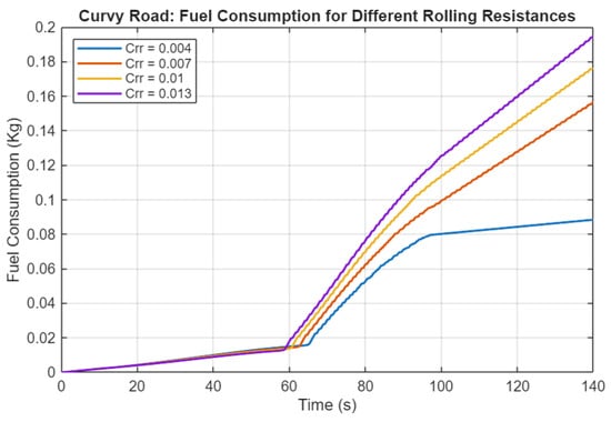
According to Table 2, the Curvy Road test generates the highest variation in fuel consumption with respect to the impact of rolling resistance. Figure 5 shows the fuel consumption behavior of the Curvy Road test for different rolling resistance coefficients. Fuel consumption is similar among all $C_{rr}$ cases during the first 60 s when the vehicle has variable longitudinal velocity. After $t=95$ s, when the vehicle maintains a constant velocity of 35 km/h, the test with $C_{rr}=0.004$ starts to stabilize fuel consumption, whereas the tests with higher $C_{rr}$ values continue increasing at a faster rate throughout the test. Even fuel consumption results in being almost twice that of $C_{rr}=0.013$ compared to the benchmark case.

Figure 5. Fuel consumption variations due to the rolling resistance coefficient.

In addition to fuel consumption, a similar analysis of engine torque was carried out with the results shown in Table 3. It can be observed that increasing the $C_{rr}$ also increases the engine torque, so the motor requires more work to complete the tests. The only exception is the Full Throttle Acceleration test, which shows a reduction in engine torque. This phenomenon is related to the velocity, which is discussed in the following paragraphs.

Table 3. Percentage changes in AUC of motor torque with respect to $C_{rr}=0.004$.

Drive Test	${\mathit{C}}_{\mathit{r}\mathit{r}}=0.007$	${\mathit{C}}_{\mathit{r}\mathit{r}}=0.01$	${\mathit{C}}_{\mathit{r}\mathit{r}}=0.013$
UDDS HD	7.65%	16.57%	24.21%
FTP-75	6.08%	11.73%	18.25%
Curvy Road	22.59%	45.37%	68.70%
Looped Road with Banking	9.81%	18.94%	23.59%
Full Throttle Acceleration (6% grade)	−1.86%	−3.67%	−1.71%

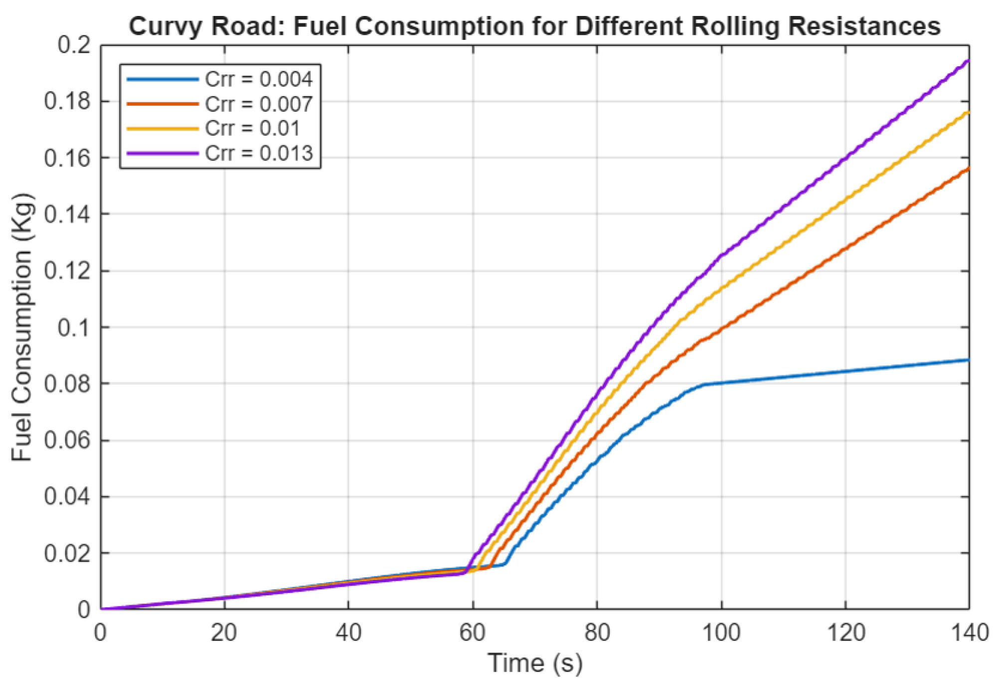
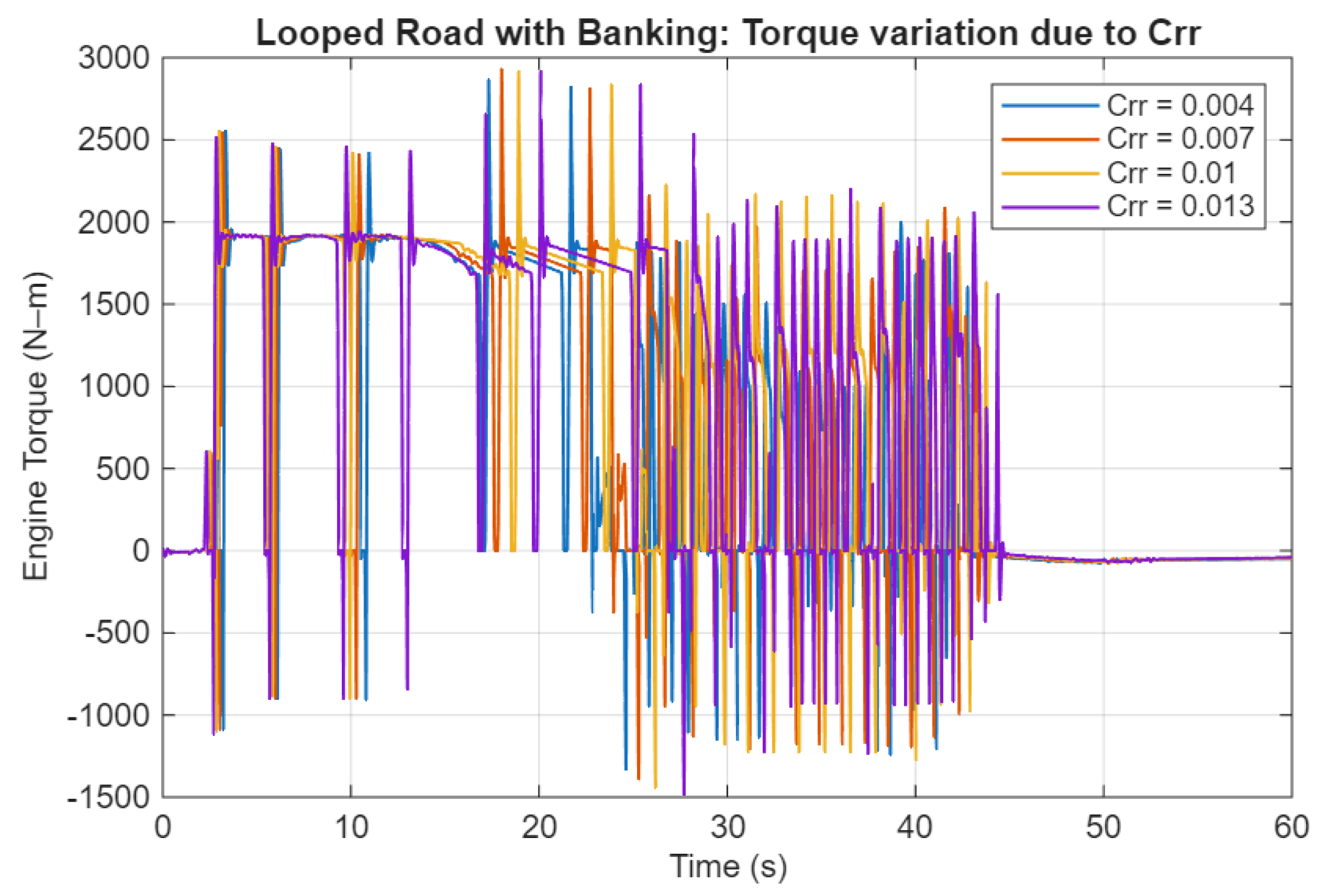
Figure 6 illustrates, as an example, the engine torque performance of the vehicle on the Looped Road with Banking test at different rolling resistance coefficients. Qualitatively, the difference is more notable around $t=20$, where the engine torque increases when $C_{rr}$ increases.

Figure 6. Variations of the engine torque due to change in rolling resistance.

Another variable affected by the change in rolling resistance is the vehicle’s speed, which decreased across all test procedures, as shown in Table 4. The UDDS HD test overall speed was the least impacted, while the Full Throttle Acceleration test was the most impacted, reaching a reduction of up to 7.57%.

Table 4. Percentage changes in AUC of the vehicle’s longitudinal velocity with respect to $C_{rr}=0.004$.

Drive Test	${\mathit{C}}_{\mathit{r}\mathit{r}}=0.007$	${\mathit{C}}_{\mathit{r}\mathit{r}}=0.01$	${\mathit{C}}_{\mathit{r}\mathit{r}}=0.013$
UDDS HD	−0.25%	−0.47%	−0.84%
FTP-75	−0.56%	−1.19%	−1.94%
Curvy Road	−2.25%	−4.21%	−5.93%
Looped Road with Banking	−1.39%	−2.85%	−4.57%
Full Throttle Acceleration (6% grade)	−3.38%	−3.41%	−7.57%

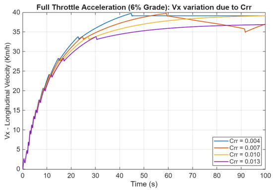
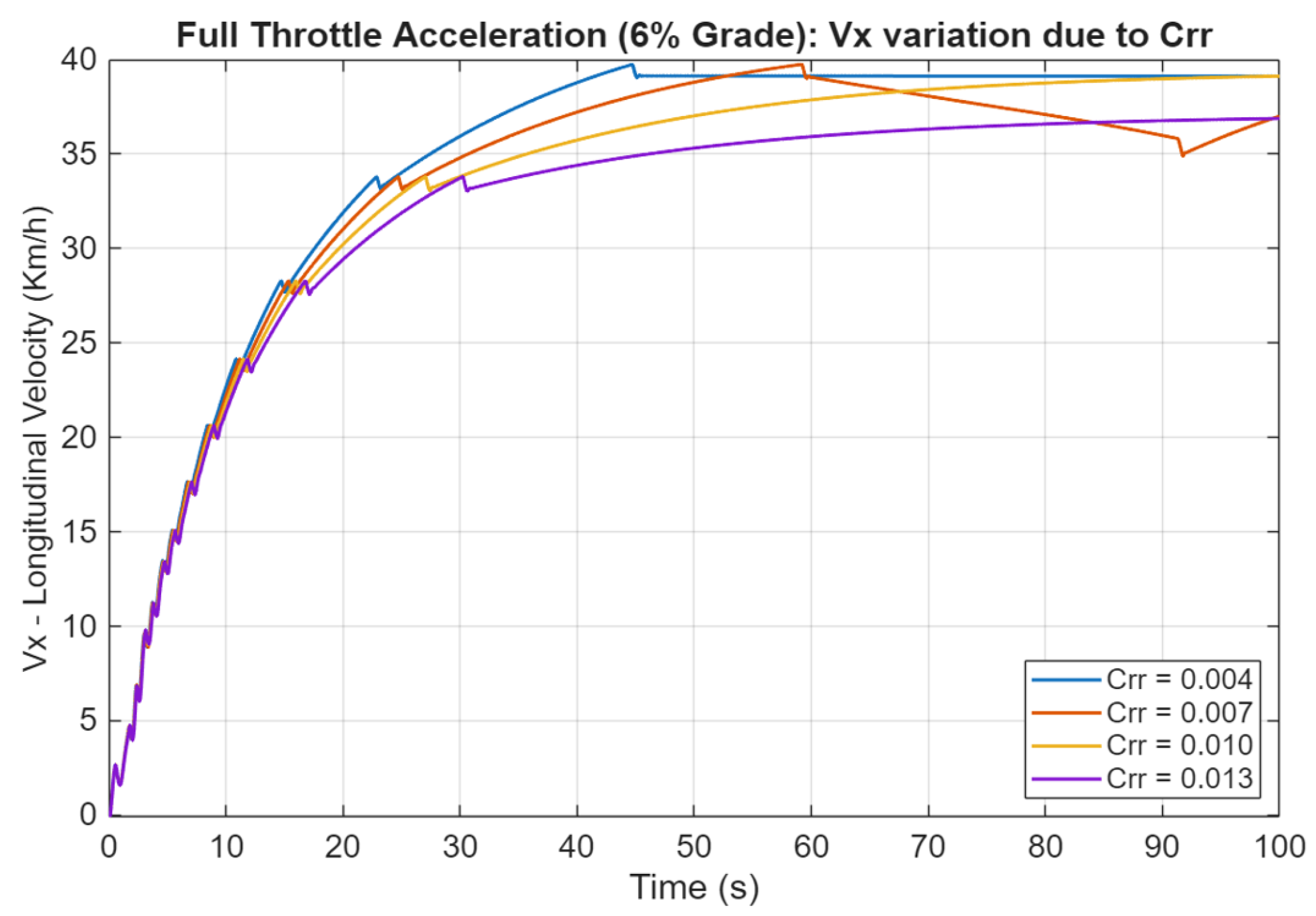
Figure 7 shows the Full Throttle Acceleration test procedure and how the vehicle’s speed changed when varying $C_{rr}$. The test results show that the vehicle’s speed increases rapidly at the start, with higher rolling resistance ($C_{rr}$) leading to a slower acceleration. As time progresses, the speed gradually levels off, with lower $C_{rr}$ values reaching higher final speeds. In particular, the figure shows that the speed with a $C_{rr}$ of 0.007 exhibits fluctuations in velocity, starting around the 60-s mark, which deviates from the smoother changes in speed shown by the other simulations.

Figure 7. Variations of the longitudinal velocity caused by the change in rolling resistance.

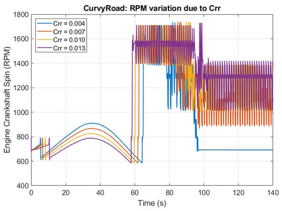
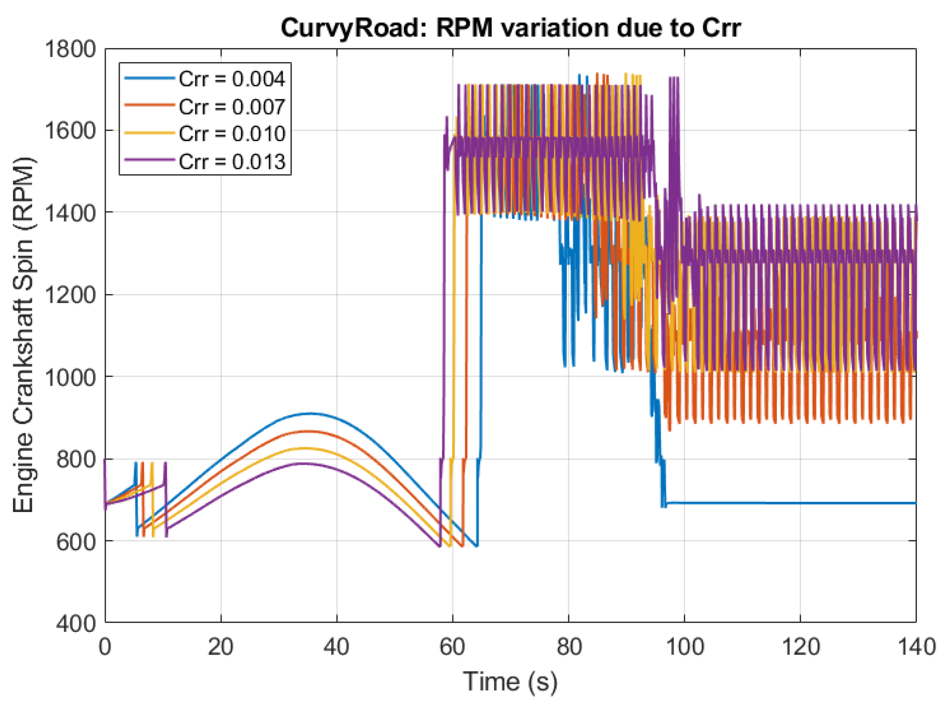
On the other hand, the engine crankshaft spin increased with the $C_{rr}$, as shown in Table 5. The test procedure that shows the biggest change due to $C_{rr}$ is the Curvy Road, as it reaches up to a 25.30% increase in rpm. The rest of the driving procedures were less affected, with the highest increase being 6.33% for the Looped Road with Banking test. Focusing on the Curvy Road test, Figure 8 shows the rpm variations due to $C_{rr}$, and it can be observed that with a $C_{rr}=0.004$, the engine crankshaft spin falls around the 95 s mark until it reaches a value of around 700 RPM, where it stabilizes. In contrast, the other tests continue oscillating for the rest of the test and never reach a lower RPM than 850. This difference in behavior explains why this test, in particular, showed the largest percentage changes in RPM.

Table 5. Percentage changes in AUC of motor’s RPM with respect to $C_{rr}=0.004$.

Drive Test	${\mathit{C}}_{\mathit{r}\mathit{r}}=0.007$	${\mathit{C}}_{\mathit{r}\mathit{r}}=0.01$	${\mathit{C}}_{\mathit{r}\mathit{r}}=0.013$
UDDS HD	0.70%	1.71%	2.38%
FTP-75	1.88%	3.44%	5.08%
Curvy Road	16.05%	23.07%	25.30%
Looped Road with Banking	1.76%	3.04%	6.33%
Full Throttle Acceleration (6% grade)	1.72%	8.24%	4.75%

Figure 8. Variations of the engine crankshaft spin due to a change in rolling resistance.

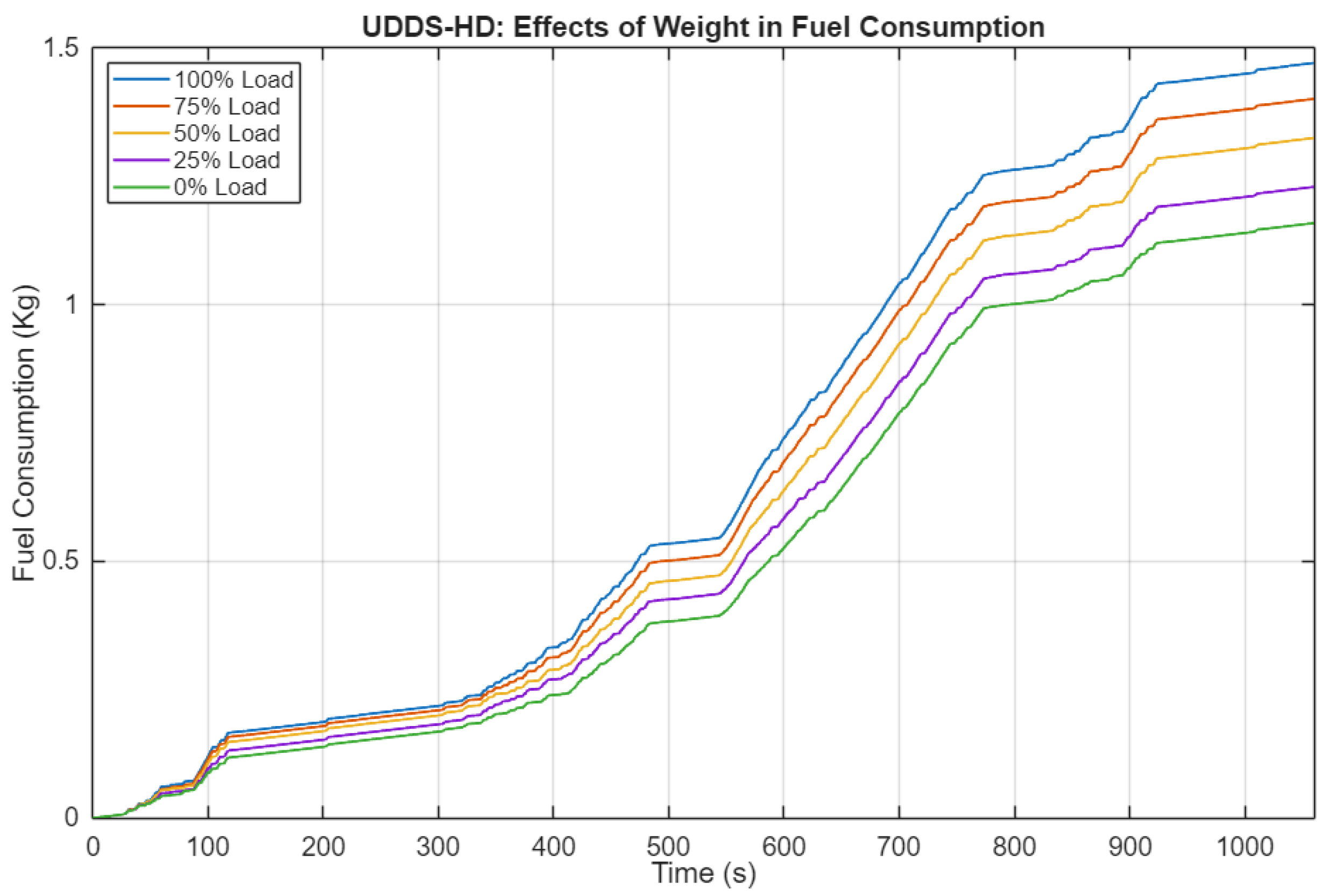
Additional simulations were conducted to analyze the impact of trailer weight on fuel consumption by considering 75%, 50%, 25% and 0% load gradients for the trailer’s payload. Figure 9 shows the simulation results of the UDDS HD cycle, for five different trailer loads using the same $C_{rr}$ value of 0.007, and by calculating the AUC the results show that a weight reduction of 50% results in a total reduction of 10.91% in fuel consumption, while reducing the load to 0% achieves a fuel consumption reduction of 23.38%. Thus, the impact of the load on fuel consumption is nonlinear.

Figure 9. UDDS HD drive cycle observed effects of load reduction in fuel consumption.

This last case study was repeated for the other drive cycles and rolling resistance values, with the results summarized in Table 6. Simulations indicate that, at best, a reduction in fuel consumption of up to approximately 30% can be achieved when the trailer is unloaded. An outlier in these results is the Full Throttle Acceleration test, which showed an increase in fuel consumption for rolling resistance coefficients ($C_{rr}$) of 0.004 and 0.007, but showed a reduction in fuel consumption at higher rolling resistance values.

Table 6. Effect of trailer weight on fuel consumption with respect to a full load.

Drive Test	Load	${\mathit{C}}_{\mathit{r}\mathit{r}}=0.004$	${\mathit{C}}_{\mathit{r}\mathit{r}}=0.007$	${\mathit{C}}_{\mathit{r}\mathit{r}}=0.010$	${\mathit{C}}_{\mathit{r}\mathit{r}}=0.013$
FTP-75	75%	−6.6947%	−5.8306%	−6.0183%	−6.3305%
	50%	−12.8045%	−13.5923%	−13.0355%	−13.5902%
	25%	−20.2440%	−20.5798%	−21.2731%	−20.8824%
	0%	−28.2441%	−27.5631%	−28.2238%	−28.8502%
UDDS HD	75%	−2.8927%	−5.0971%	−6.3239%	−5.9325%
	50%	−10.9145%	−10.9104%	−12.0035%	−13.1977%
	25%	−16.3083%	−17.6351%	−20.1885%	−19.4480%
	0%	−22.5961%	−23.3821%	−25.7406%	−27.1970%
Curvy Road	75%	−3.1683%	−6.5005%	−6.4774%	−7.8648%
	50%	−12.2014%	−8.2713%	−13.9073%	−15.0133%
	25%	−19.1418%	−27.9416%	−20.4361%	−21.4991%
	0%	−26.6877%	−24.8132%	−30.3935%	−28.2515%
Looped Road with Banking	75%	−7.1384%	−6.7809	−6.7739%	−7.6716%
	50%	−12.5263%	−15.2028%	−14.6243%	−15.4201%
	25%	−23.4702%	−20.0886%	−23.6627%	−24.3208%
	0%	−20.8239%	−27.9447%	−28.0930%	−30.1929%
Full Throttle Acceleration (6% grade)	75%	3.0514%	0.4184%	−3.7664%	−2.2137%
	50%	3.4869%	0.2454%	−3.2778%	−0.9527%
	25%	2.3097%	−0.2566%	−3.5512%	−1.4562%
	0%	1.0252%	−1.0914%	−2.8815%	−1.2898%

The weight also has an important effect on the engine torque, with the results in Table 7 illustrating that the engine can relax in torque up to 46% when the weight of the cargo is 0%, in this case, considering the Looped Road with Banking test. These results show that the torque exhibits a pretty similar rate of change when varying the load and $C_{rr}$ for the FTP-75, UDDS HD, and Curvy Road tests. A relaxation is also observed in the engine crankshaft spin with up to 19% in the Looped Road with Banking and Curvy Road tests, see Table 8. However, in both cases, the Full Throttle Acceleration test does not follow the same trend, as it shows an increase in torque rather than a decrease with $C_{rr}$ values of 0.010 and 0.013, and an increase in engine RPMs with the two lower $C_{rr}$ values.

Table 7. Effect of trailer weight on engine torque with respect to a full load.

Drive Test	Load	${\mathit{C}}_{\mathit{r}\mathit{r}}=0.004$	${\mathit{C}}_{\mathit{r}\mathit{r}}=0.007$	${\mathit{C}}_{\mathit{r}\mathit{r}}=0.010$	${\mathit{C}}_{\mathit{r}\mathit{r}}=0.013$
FTP-75	75%	−8.5032%	−8.7394%	−7.9282%	−8.7457%
	50%	−17.0270%	−17.4986%	−17.0529%	−17.3105%
	25%	−25.7001%	−26.3336%	−26.3252%	−26.6084%
	0%	−34.7750%	−35.7948%	−35.7653%	−36.3072%
UDDS HD	75%	−7.5281%	−7.1386%	−7.9274%	−8.2488%
	50%	−16.3746%	−16.3121%	−17.6056%	−17.5299%
	25%	−26.3499%	−26.5535%	−27.9421%	−27.8759%
	0%	−34.7472%	−35.5713%	−37.3464%	−37.7441%
Curvy Road	75%	−6.4169%	−8.8814%	−9.0248%	−15.2177%
	50%	−12.4333%	−16.9532%	−17.5271%	−18.9673%
	25%	−19.7276%	−22.3879%	−27.0661%	−24.4702%
	0%	−19.9681%	−35.1669%	−35.6948%	−35.6491%
Looped Road with Banking	75%	−8.4105%	−10.9440%	−11.6028%	−9.9920%
	50%	−22.3824%	−22.6137%	−22.3753%	−19.8581%
	25%	−33.6719%	−33.4802%	−33.4835%	−31.3179%
	0%	−45.0998%	−46.9189%	−46.6244%	−44.0982%
Full Throttle Acceleration (6% grade)	75%	−2.3110%	−1.1246%	2.4731%	1.8346%
	50%	−3.6900%	−1.2502%	1.9162%	0.7592%
	25%	−4.1616%	−2.3682%	0.6582%	−0.4664%
	0%	−3.9206%	−3.3862%	−2.3322%	−3.2136%

Table 8. Effect of trailer weight on engine crankshaft spin with respect to a full load.

Drive Test	Load	${\mathit{C}}_{\mathit{r}\mathit{r}}=0.004$	${\mathit{C}}_{\mathit{r}\mathit{r}}=0.007$	${\mathit{C}}_{\mathit{r}\mathit{r}}=0.010$	${\mathit{C}}_{\mathit{r}\mathit{r}}=0.013$
FTP-75	75%	−1.5439%	−1.3835%	−1.4826%	−1.4308%
	50%	−3.0877%	−3.7005%	−3.4208%	−3.5446%
	25%	−5.5870%	−5.7485%	−5.9890%	−5.9393%
	0%	−8.6826%	−8.6882%	−9.2252%	−9.6272%
UDDS HD	75%	−0.1009%	−1.2480%	−1.5558%	−1.0779%
	50%	−1.9155%	−2.0319%	−2.3129%	−2.7352%
	25%	−3.1022%	−3.0860%	−3.8628%	−3.7268%
	0%	−4.7754%	−5.1179%	−5.3552%	−5.7939%
Curvy Road	75%	−0.9972%	−1.6145%	−2.0945%	−0.3823%
	50%	−3.8999%	−10.8477%	−6.6337%	−3.6800%
	25%	−4.1998%	−15.3034%	−9.8702%	−10.6437%
	0%	−7.2975%	−16.8234%	−11.8358%	−19.1496%
Looped Road with Banking	75%	−6.3062%	−1.8594%	−2.4608%	−3.3300%
	50%	−10.9971%	−4.8294%	−5.0309%	−6.6307%
	25%	−12.6886%	−15.6999%	−7.8474%	−9.9453%
	0%	−19.0254%	−16.0428%	−13.5492%	−10.9010%
Full Throttle Acceleration (6% grade)	75%	4.5409%	4.6706%	−4.4754%	−3.8008%
	50%	6.7206%	4.4558%	−4.0082%	−2.3003%
	25%	6.2622%	5.1206%	−3.0851%	−1.3597%
	0%	4.9933%	4.1196%	0.1152%	1.8042%

Finally, analyzing the impact of weight on the longitudinal velocity of the vehicle seems to be more critical for the Full Throttle Acceleration test, as Table 9 illustrates, with an increase of up to 86% when the trailer’s load is 0%. However, the longitudinal velocity is slightly affected by the rolling resistance coefficient when the weight changes, i.e., each test shows slight differences in $V_x$ when $C_{rr}$ changes. UDDS HD and Curvy Road barely show a difference, while the FTP-75 test increases 5.06%, and Looped Road with Banking increases up to 9.01% at best.

Table 9. Effect of trailer weight on the vehicle’s speed with respect to a full load.

Drive Test	Load	${\mathit{C}}_{\mathit{r}\mathit{r}}=0.004$	${\mathit{C}}_{\mathit{r}\mathit{r}}=0.007$	${\mathit{C}}_{\mathit{r}\mathit{r}}=0.010$	${\mathit{C}}_{\mathit{r}\mathit{r}}=0.013$
FTP-75	75%	1.1977%	1.3354%	1.5107%	1.7687%
	50%	2.1811%	2.4641%	2.8521%	3.4016%
	25%	2.8599%	3.2667%	3.6925%	4.3436%
	0%	3.4399%	3.9040%	4.4656%	5.0632%
UDDS HD	75%	0.4055%	0.3948%	0.4599%	0.6085%
	50%	0.4909%	0.5844%	0.6976%	0.9517%
	25%	0.5098%	0.6962%	0.8220%	1.1214%
	0%	0.4400%	0.5978%	0.7763%	1.0590%
Curvy Road	75%	0.2268%	0.0515%	0.1291%	0.1995%
	50%	0.6353%	0.1152%	0.2760%	0.4328%
	25%	0.9950%	0.3968%	0.4562%	0.7453%
	0%	1.7091%	0.2301%	0.6789%	1.1479%
Looped Road with Banking	75%	2.2312%	2.4232%	2.7021%	3.4531%
	50%	4.1280%	4.8368%	5.3760%	6.3579%
	25%	5.9385%	6.6176	7.4863%	8.4885%
	0%	6.2939%	7.0371	7.7955%	9.0173%
Full Throttle Acceleration (6% grade)	75%	15.6268%	16.2018%	11.4657%	11.7334%
	50%	33.5362%	33.6854%	28.9218%	30.2211%
	25%	55.1396%	56.3099%	51.5284%	53.5708%
	0%	84.7795%	85.7732%	83.0206%	86.3979%

Overall, the simulation results show that for standard road profiles, such as FTP-75 and UDDS HD, the impact of load on fuel consumption is notable: Heavy-duty vehicles can increase fuel consumption by around 25% when the trailer is fully loaded. This increase can be slightly higher for curvy and banked roads. On the other hand, the impact of $C_{rr}$ on fuel consumption is less influential than the load effect; but, when the HDV is unloaded, the increasing on the rolling resistance generates more fuel consumption, especially for the UDDS HD and Looped Road with Banking tests, and this increasing of fuel consumption is slighter for the FTP-75 road. Due to the unusual engine demands of the Full Throttle Acceleration test, the relationship between load, $C_{rr}$, and fuel consumption is highly nonlinear and complex. In this latter case, fuel consumption seems to be more dependent on the driving conditions considered in the test than on a pattern between weight and rolling resistance.

These results highlight the importance of monitoring the fuel and energy efficiency on heavy-duty vehicles at real driving conditions through telemetry at different experimental scenarios, and specifically how the tire technology can influence the reduction in fuel consumption [22], and even more, the reduction of greenhouse gas emissions. In [22], it is stated that tire technology can reduce fuel consumption by around 3% compared to other tire technologies on HDVs, and this reduction is 3–4 times greater when good driving habits are used with an Advanced Driver Assistance System.

5. Conclusions

In this work, a simulation-based analysis of the impact of rolling resistance on fuel economy has been conducted, yielding the following key insights. First, fleets driving on the same roads with different tire technologies (different $C_{rr}$) will show different fuel consumption. In this research, the increase in $C_{rr}$ resulted in up to 68.01% more fuel consumption. Additionally, with more $C_{rr}$, the tractor and trailer are slower, with the results showing a reduction in speed of up to 7.57%, implying that drivers will accelerate more to reach the final destination in the same time, as a consequence: (i) higher fuel consumption, (ii) greater wear of the engine and powertrain, (iii) on curvy roads with banks and slopes, the effect could be five times larger. Furthermore, $C_{rr}$ affects the applied torque proportionally, as seen in the Curvy Road scenario, which shows the highest torque increase (68.70%) as the engine compensates for the added drag of the tires. This shows that mechanical component energy losses can increase, and that higher $C_{rr}$ has a multiplicative effect on energy consumption under specific driving conditions (acceleration/braking). Finally, load variation simulations suggest that the influence of $C_{rr}$ on fuel consumption can be validated without specific information on tractor loads in the fleets, since the percentage of fuel consumption attributable to $C_{rr}$ is almost the same for the different cases. While the findings of this work are expected to generalize qualitatively across different scenarios, the quantitative results reported are vehicle model-dependent. However, the use of the TruckSim modeling approach enables the repeatability of these tests across other specific tractor-trailer configurations and components, such as tire parameters, trailer payload, and surrounding environmental conditions. The simulation platform’s modularity provides a standardized framework for future works to explore more complex tire models, due to the integrated support for user defined models as well as the use of third party models like COSIN’s FTire or SIEMENS MF-Tyre and MF-Swift models, so subsequent works could account for transient effects like tire temperatures and inflation pressure, in addition to the use of driving cycles more in accordance with the geographical conditions in Mexico. In addition, future work should validate the impact of tire rolling resistance on real Class 8 tractor-trailer fuel consumption, considering tire operational variables, and the impact of tires with different rolling resistances on Mexican fleets’ operational costs.

References

- European Environment Agency. Climate: Sustainability of Europe’s Mobility Systems; Report Web Report No. 01/2024; European Environment Agency: Copenhagen, Denmark, 2024. [Google Scholar] [CrossRef]
- U.S. Environmental Protection Agency. Inventory of U.S. Greenhouse Gas Emissions and Sinks: 1990–2022; Technical Report EPA 430-R-24-004; U.S. Environmental Protection Agency: Washington, DC, USA, 2024.
- Present, S.; Rexeis, M. Potential Assessment of Electrified Heavy-Duty Trailers Based on the Methods Developed for EU Legislation (VECTO Trailer). Future Transp. 2025, 5, 77. [Google Scholar] [CrossRef] [Scilit]
- Trucks, D. Recovery Act–Class 8 Truck Freight Efficiency Improvement Project; Technical Report; Daimler Trucks North America LLC: Portland, OR, USA, 2015. [Google Scholar] [CrossRef] [Scilit]
- Aldhufairi, H.S.; Olatunbosun, O.A. Developments in tyre design for lower rolling resistance: A state of the art review. Proc. Inst. Mech. Eng. Part D J. Automob. Eng. 2018, 232, 1865–1882. [Google Scholar] [CrossRef] [Scilit]
- Ydrefors, L.; Hjort, M.; Kharrazi, S.; Jerrelind, J.; Trigell, A.S. Rolling resistance and its relation to operating conditions: A literature review. Proc. Inst. Mech. Eng. Part D J. Automob. Eng. 2021, 235, 2931–2948. [Google Scholar] [CrossRef] [Scilit]
- Srirangam, S.K.; Anupam, K.; Kasbergen, C.; Scarpas, A.; Cerezo, V. Study of Influence of Operating Parameters on Braking Friction and Rolling Resistance. Transp. Res. Rec. 2015, 2525, 79–90. [Google Scholar] [CrossRef] [Scilit]
- Ejsmont, J.; Taryma, S.; Ronowski, G.; Swieczko-Zurek, B. Influence of load and inflation pressure on the tyre rolling resistance. Int. J. Automot. Technol. 2016, 17, 237–244. [Google Scholar] [CrossRef] [Scilit]
- Song, J. Evaluation of driving resistance and energy consumption in electric vehicles under various ambient and tire temperatures using real-world driving data. Transportation 2025, 25, 100454. [Google Scholar] [CrossRef] [Scilit]
- Świeczko-Żurek, B.; Ronowski, G.; Ejsmont, J. Tyre rolling resistance and its influence on fuel consumption. Combust. Engines 2017, 168, 62–67. [Google Scholar] [CrossRef] [Scilit] [PubMed]
- Na, X.; Cebon, D. Quantifying fuel-saving benefit of low-rolling-resistance tyres from heavy goods vehicle in-service operations. Transp. Res. Part D Transp. Environ. 2022, 113, 103501. [Google Scholar] [CrossRef] [Scilit]
- Liu, Q.; Pei, J.; Wang, Z.; Hu, D.; Huang, G.; Meng, Y.; Lyu, L.; Zheng, F. Analysis of tire-pavement interaction modeling and rolling energy consumption based on finite element simulation. Constr. Build. Mater. 2024, 425, 136101. [Google Scholar] [CrossRef] [Scilit]
- Bachman, L.J. Do Changes in Temperature and Inflation Pressure Affect Rolling Resistance during Road and Track Testing for Fuel Economy of Class 8 Tractor-Trailers? Tire Sci. Technol. 2018, 46, 93–104. [Google Scholar] [CrossRef] [Scilit] [PubMed]
- Rahkola, P. Driving Resistance Measurements of Heavy-Duty Vehicles; Number VTT-R-00316-25 in VTT Research Report; 2609/31/2022, 133808/No Damage; VTT Technical Research Centre of Finland: Espoo, Finland, 2025. [Google Scholar]
- Société de Technologie Michelin. The Tyre: Rolling Resistance and Fuel Savings; 23 rue Breschet, C.F., Ed.; Société de Technologie Michelin: Clermont-Ferrand, France, 2003. [Google Scholar]
- Bakker, E.; Pacejka, H.B.; Lidner, L. A New Tire Model with an Application in Vehicle Dynamics Studies; Technical Report 890087; SAE Technical Paper: Warrendale, PA, USA, 1989. [Google Scholar]
- Pacejka, H.; Sharp, R. Shear Force Development by Pneumatic Tyres in Steady State Conditions: A Review of Modelling Aspects. Veh. Syst. Dyn. 1991, 20, 121–175. [Google Scholar] [CrossRef] [Scilit]
- Hamilton, D.; Sessions, J.; Langevin, C. Identifying rolling resistance and air resistance simultaneously for an electric truck. Int. J. For. Eng. 2025, 1–15. [Google Scholar] [CrossRef] [Scilit]
- Nakajima, Y. Rolling Resistance of Tires. In Advanced Tire Mechanics; Springer: Singapore, 2019. [Google Scholar]
- Giakoumis, E.G.; Zachiotis, A.T. A comprehensive comparative investigation of a heavy-duty vehicle’s performance, consumption and emissions during eight driving cycles. Int. J. Ambient Energy 2021, 42, 29–45. [Google Scholar] [CrossRef] [Scilit]
- Gebisa, A.; Gebresenbet, G.; Gopal, R.; Nallamothu, R.B. Driving Cycles for Estimating Vehicle Emission Levels and Energy Consumption. Future Transp. 2021, 1, 615–638. [Google Scholar] [CrossRef] [Scilit]
- Treviño, R. Cuando la Ciencia Sale a la Carretera: Investigadores Comprueban la Eficiencia de un Neumático Michelin; Transformación Industrial, TecSience, Tecnológico de Monterrey: Monterrey, Mexico, 2025. [Google Scholar]
Disclaimer/Publisher’s Note: The statements, opinions and data contained in all publications are solely those of the individual author(s) and contributor(s) and not of MDPI and/or the editor(s). MDPI and/or the editor(s) disclaim responsibility for any injury to people or property resulting from any ideas, methods, instructions or products referred to in the content. |
© 2026 by the authors. Licensee MDPI, Basel, Switzerland. This article is an open access article distributed under the terms and conditions of the Creative Commons Attribution (CC BY) license.