Parameterized Reinforcement Learning with Route Guidance for Controlling Urban Road Traffic Networks

Abstract

Traditional macroscopic fundamental diagram (MFD)-based traffic perimeter metering control strategies rely on full knowledge of vehicle accumulation and inter-regional flow dynamics, assumptions that seldom hold in heterogeneous and highly variable real-world networks. Classical data-driven reinforcement learning methods face similar constraints, often converging slowly and exhibiting low sample efficiency when confronted with such complexities. Motivated by these limitations, this paper proposes a Parameterized Deep Q-Network perimeter control (P-DQNPC) scheme designed for multi-region urban road networks. The framework jointly optimizes discrete actions (regional routing choices) and continuous actions (signal-timing or flow-duration regulation) within a model-free learning structure. The approach is first trained and validated on synthetic MFD data to establish stable and interpretable policy behavior under controlled conditions. It is then transferred and further evaluated using real-world measurements from the Performance Measurement System—San Francisco Bay Area (PeMS-SF), a dataset collected from 18,954 loop detectors across the California State Highway System. PeMS-SF is selected due to its high spatial and temporal resolution, broad network coverage, and strong ability to capture realistic and diverse congestion patterns qualities that support both rigorous validation and generalization to other metropolitan regions. Experimental results show that P-DQNPC consistently outperforms state-of-the-art baselines, including deep deterministic policy gradient, deep Q-network, and No-Control schemes. The proposed method achieves superior regulation of regional accumulations and demonstrates enhanced robustness in large, heterogeneous, and uncertain urban traffic environments.

1. Introduction

Adaptive traffic control systems are essential for enhancing vehicular flow on urban road networks by dynamically responding to prevailing traffic conditions [1]. Among these control schemes, traffic perimeter control has shown promise in mitigating congestion at the boundary interfaces of homogeneous urban regions [2]. However, modeling large-scale traffic networks remains a complex undertaking due to the high number of links, intersections, and inherent uncertainties. The most recent empirical studies have verified that perimeter control methods can provide good performance with a well-defined macroscopic fundamental diagram (MFD) in numerical experiments [3,4]. The MFD-based perimeter control framework characterizes a unimodal, low-scatter relationship between the critical accumulation and network inflow, enabling more effective regulation of boundary flows and consequently enhancing the overall operational efficiency of urban traffic networks [5,6]. Moreover, RL enables adaptive local and network-level control, region-level strategies based on the MFD provide complementary insights by representing aggregated traffic flow–density dynamics. Recent advances in machine learning and physics-informed methods have leveraged MFDs for accurate traffic state estimation and control, including probe-data-driven predictions in North American cities [7] and graph-learning-based imputation in European networks [8]. Integrating MFD insights with adaptive control policies enhances large-scale traffic management by capturing network-level dynamics that inform more effective control strategies. However, its practical implementation remains constrained by the inherent heterogeneity of urban road networks, highlighting the need for better modeling approaches that can more accurately capture spatial variations and complex traffic flow dynamics for improved control performance. Conventional fixed-time and actuated signal control strategies struggle to manage congestion in large-scale urban networks characterized by heterogeneous demand. Reinforcement-learning-based traffic control enables adaptive, model-free optimization of signal timing and route guidance, effectively responding to real-time network dynamics and improving overall system performance [9,10]. However, such approaches may also struggle with scalability and generalization under varying demand patterns.

Perimeter control strategies are generally categorized into model-based perimeter control (MPC) and model-free adaptive control (MFAC), each differing in its reliance on traffic models and real-time data learning mechanisms [11,12]. Recent regional and hierarchical traffic control frameworks integrate MFD dynamics with advanced adaptive methods, including physics-regularized multi-agent reinforcement learning and differentiable predictive control, to optimize perimeter and network-level flows. MPC with MFD-based route guidance has also been validated in realistic European urban networks, demonstrating scalability, robustness, and transferability across heterogeneous demand patterns [13,14,15]. These studies highlight the potential of combining intersection-level reinforcement learning (RL) with aggregated network control to improve overall urban traffic performance. The implementation of MFD-based perimeter control has predominantly relied on MPC methodologies that require explicit system modeling, controller design, and simulation [16]. However, developing accurate models remains challenging due to model mismatch issues and the limited generalizability of such models across varying traffic environments [17]. To fully exploit the valuable data collected from real-world traffic systems, MFAC approaches are often favored over traditional MPC schemes, and several promising studies have been conducted in this direction [18]. The MFAC schemes are purely data-driven, nonlinear, and non-affine methods applied to perimeter control to solve the strongly coupled interconnections between subregions. The schemes have exhibited great performance in highly complex traffic flow patterns. This is due to their ability to use several virtual equivalent dynamic data models based on time-varying pseudo-partial derivatives [19,20]. Nevertheless, the performance of MFAC schemes remains constrained by the accuracy of estimated network parameters, such as critical accumulation and traffic demand, within the regional MFD framework that are embedded in the controller design. These limitations increase the model’s susceptibility to estimation errors due to multivaluedness, leading to hysteresis scatter in the MFD and potential instability under real-world traffic dynamics [21,22]. Nevertheless, when adequately trained on traffic condition data, the MFAC models are capable of solving complex traffic control problems more effectively and with less computational cost. Model-free, data-driven reinforcement learning perimeter control (MFARLPC) schemes have demonstrated considerable effectiveness in regulating traffic across regional boundaries, providing improved scalability in addressing hysteresis phenomena relative to traditional model-based MFD approaches [23,24]. Although MFARLPC schemes can regulate traffic effectively by leveraging interactions between the traffic state and control actions, classical MFARLPC schemes face substantial limitations. In particular, they suffer from the curse of dimensionality in both state and action spaces when deployed in multi-region networks. They equally lack robustness to discrete and spatiotemporal traffic variables that arise from dynamic vehicle behaviors in real-world conditions [25].

The traditional model-free based perimeter control schemes, including rule-based gating and model-predictive approaches, continue to face several persistent limitations when deployed in large, heterogeneous urban networks. Their effectiveness depends strongly on idealized MFD relationships, which can deviate significantly from real measurements in the presence of spillback, multi-modal flow interactions, or stochastic demand variations [26]. Furthermore, these strategies assume relatively smooth and stationary dynamics, making them vulnerable to abrupt changes in accumulation levels, sensor noise, and imperfect state observability issues that are especially prominent in high-resolution performance measurement systems [27,28]. As a result, traditional approaches often under-perform near critical accumulation thresholds, leading to unstable gating policies, increased total travel time, and reduced throughput when applied to multi-region perimeter control. To overcome these constraints, this paper introduces a hybrid RL framework built around a Parameterized Deep Q-Network (P-DQN) agent specifically designed for multi-region perimeter management. The proposed architecture integrates discrete gating decisions with continuous flow-rate parameterization with route guidance, allowing the controller to learn fine-grained metering actions that respect both regional MFD characteristics and real-world operational constraints. Motivated by the research gaps highlighted above, this study aims to achieve the following contributions:

• A real-time network partitioning scheme and mass-conservation traffic dynamics are embedded within the MFD framework, improving regional homogeneity and enhancing trip completion rates under varying congestion levels.
• A model-free Parameterized Deep Q-Network Perimeter Control (P-DQNPC) framework is developed to jointly optimize hybrid actions, combining discrete route-direction decisions with continuous flow-regulation controls for flexible and effective perimeter metering.
• A two-stage learning pipeline is introduced, where P-DQNPC is first trained on synthetic MFD-generated data to acquire stable control policies, and subsequently evaluated on real-world PeMS measurements to validate transferability and robustness in heterogeneous traffic conditions.
• Extensive experiments demonstrate that P-DQNPC achieves faster convergence, higher data efficiency, and superior congestion mitigation compared to classical RL baselines, i.e., deep Q-network (DQN), No-Control (NC) and deterministic policy gradient (DDPG), effectively addressing estimation errors, hysteresis scatter, and dynamic variability in large-scale urban networks.

The paper is organized as follows: Section 2 reviews the relevant literature and identifies existing research gaps. Section 3 presents the generalized urban traffic system model, including detailed mathematical models. Section 4 presents the experimental setup. Section 5 shows the experimental results and evaluates the performance of P-DQN on synthetic and real world PeMS data. Finally, Section 6 concludes the paper and outlines directions for future research.

2. Related Works

Classical perimeter control schemes are inherently model-dependent and sensitive to modeling uncertainties and disturbances. To address these challenges, an MFD-based integral RL framework is thus developed in [29], employing an actor–critic neural network to adaptively approximate traffic dynamics for optimal perimeter control. Convergence and stability of the frameworks is guaranteed through the application of the Lyapunov optimization strategy. However, its application to large-scale nonlinear systems introduces substantial computational challenges. To address the traffic flow dynamics associated with regional congestion, the authors in [30] proposed MFD-based perimeter control schemes using Q-learning and DDPG methods. These approaches aim to solve the control problem without relying on explicit traffic model information. Although the algorithms converged rapidly to a stable state and achieved superior performance in optimizing regional perimeter control, their applicability remains limited to small-scale urban networks. In [31], model-free data-driven traffic perimeter control is formulated as an RL problem and solved using the proximal policy optimization (PPO) algorithm. It is formulated to optimize homogeneous traffic flow at the border of a protected region using a microscopic framework. Although the model exhibited enhanced transferability and scalability. However, the performance of the proximal policy optimization (PPO) algorithm is strongly influenced by tuning factors such as learning rate, batch size, number of epochs, and clipping range, which can result in suboptimal traffic control decision policies. To address the state action dimensionality challenges in large-scale multi-region urban networks, the authors in [32] proposed a highly scalable model-free multi-agent deep reinforcement learning algorithm (SMF-MARL). The system clusters traffic regions into coherent zones with embedded MARL agents. Furthermore, the SMF-MARL framework decomposes the Q-value function parameters through centralized training and decentralized execution, thereby alleviating the state–action dimensionality burden. However, the study did not account for environmental uncertainties, indicating the need for additional sensitivity analysis to validate the model’s resilience. The authors in [33] proposed a model-free, data-driven reinforcement learning (MFDDRL)-based traffic control scheme to regulate traffic flow across the borders of two regions of an urban network. The MFDDRL framework dynamically adjusts control variables based on the cell transmission model. Furthermore, each of the four regions is developed with variable MFD traffic parameterization. Validation further shows that model can adapt better to new traffic environment scenarios than model-based ones, yet scalability and generalization remain a challenge. In [34], the authors developed a model-free deep reinforcement learning-based perimeter control (MFDRLPC) scheme designed to regulate traffic flow across a two-region urban network. Its key limitation lies in the reliance on two distinct RL agents, i.e., continuous reinforcement and discrete reinforcement, which limits its ability to effectively manage hybrid action spaces.

Across the reviewed studies, several observations emerge. Early work presented in [33,34] demonstrated the feasibility of model-free reinforcement learning for perimeter metering, but their frameworks remain constrained by simplified traffic dynamics: two-region network assumptions, and limited handling of stochastic variability. More recent research, including [29,30,31,32], has advanced the field through data-efficient RL schemes, multi-agent coordination, and deep policy optimization. Nevertheless, persistent challenges remain, particularly the curse of dimensionality in multi-region environments, instability of continuous-action deep reinforcement learning methods, sensitivity to MFD estimation errors, and limited scalability to large urban networks. These limitations are collectively highlighted the need for perimeter control schemes that can:

• Adapt to discrete and temporally varying real-world conditions;
• Efficiently handle high-dimensional state–action spaces;
• Maintain stability across heterogeneous regions;
• Provide robustness to imperfect sensing and dynamic vehicle behaviors.

Such gaps directly motivate the development of more flexible, parameterized action architectures and hybrid RL strategies capable of addressing the complexities of real-world multi-region urban traffic environments. The P-DQN perimeter control architecture unifies discrete gating decisions and continuous metering-rate adjustments within a single agent, effectively overcoming the challenges associated with hybrid action spaces. Its parameterized action structure enables fine-grained control adaptability while preserving computational efficiency for multi-region networks. Furthermore, by learning directly from real-world PeMS-SF traffic measurements, the proposed P-DQN controller exhibits superior scalability, enhanced robustness to environmental uncertainties, and improved responsiveness to dynamic congestion patterns offering a practical and high-performing alternative to existing classical and model-free RL schemes.

3. A Generalized Urban Traffic System Model

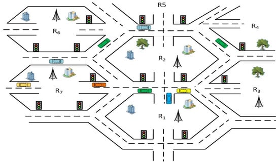
Figure 1 illustrates a generalized urban road network subdivided into seven regions, with the central region $\mathrm{R}2$ representing the city center.

Figure 1. Schematic diagram of urban traffic model.

The central region typically experiences high inflow during morning peak hours, as commuters travel to work and business centers, and heavy outflow during evening peak hours, as traffic congestion surges toward residential areas. The network is modeled to dynamically manage traffic flows: for instance, when the inflow from an outer region such as $\mathrm{R}1$ toward $\mathrm{R}2$ (city center) becomes excessive, the system reconfigures traffic by redirecting vehicles through alternative subregions (e.g., $\mathrm{R}3$ and $\mathrm{R}7$) to mitigate congestion towards city center. This traffic reconfiguration logic is applied symmetrically across all other regions, enabling adaptive load balancing throughout the urban network. Table 1 shows the frequently used symbols and acronyms and their full description that will be frequently used in this section.

Table 1. List and definition of acronyms.

Symbol	Description
$G_i\left(n_i\left(t\right)\right)$	Trip completion flow of region i at time step t
$M_{iii}$	Internal transfer (exit) flow of region i
$M_{ikj}$	Transfer flow from region i to region j via intermediate region k
$M_{kij}$	Transfer flow entering from region k, passing through region i, with destination region j
$n_i\left(t\right)$	Total vehicle accumulation in region i at time step t
$n_{ii},n_{ij}$	Vehicle accumulation traveling from region i to region i or j
${\theta }_{ikj}$	Route choice proportion for vehicles traveling from region i to j via region k
$q_{ii},q_{ij}$	Traffic demand from region i to region i or j
$R_i$	Region i
$⟨\mathcal{S},\mathcal{A},\mathcal{R},\pi ⟩$	Markov Decision Process (MDP) tuple stored in the replay memory
$t_{ikj}$	Travel time from region i to region j via region k
$u_{ij}\left(t\right)$	Perimeter control ratio from region i to region j at time step t

3.1. Three-Region Traffic System Model

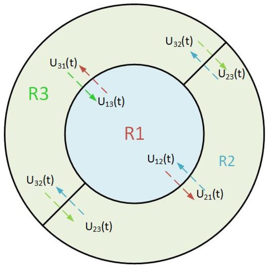
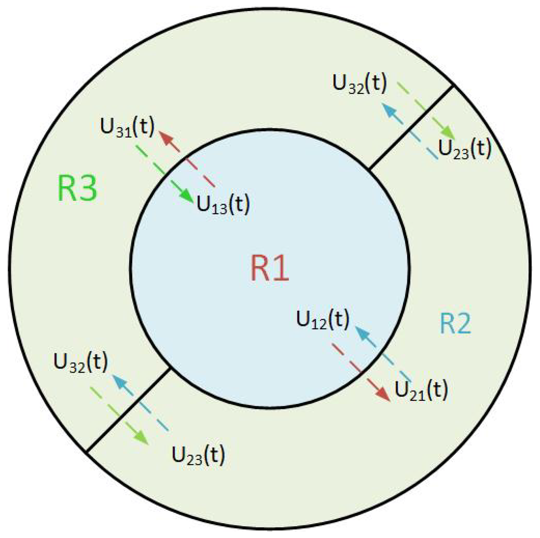
In this study, the three aggregated regions are considered, as shown in Figure 2, to clearly demonstrate how route choice can be implemented while keeping the model simple. Importantly, the proposed P-DQNPC framework is fully generalizable and can be applied to any number of regions, allowing future extension to more complex urban networks without changing the underlying methodology. From the generalized traffic road network of Figure 1, lets consider $\mathcal{N}=1,\dots ,N$ number of heterogeneous regions, partitioned into $N=\left\{1,\dots ,\mathrm{R}\right\}$ homogeneous subregions, as shown in Figure 2. The proposed traffic perimeter control strategy is developed to regulate the traffic flow in and out of protected region.

Figure 2. A three-region homogeneous perimeter control traffic model.

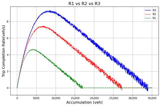
Note that region 1 $\left(\mathrm{R}1\right)$ is considered to be the most dense protected inner region, (i.e., city center) which typically experiences high transfer demand from adjacent regions. Similarly, $u_{ij}\left(t\right)$, $(i,j=1,2,3)$ denotes the perimeter control variables for the three regions (i.e., $u_{12}$ is the perimeter control of the traffic flow across the boundary of region $\mathrm{R}1$ and region $\mathrm{R}2$); this concept is implied to the borders of other regions (i.e., $\mathrm{R}1$ and $\mathrm{R}3$ or $\mathrm{R}2$ and $\mathrm{R}3$), respectively. Each of the regions characterized by a distinct MFD as shown by Figure 3. The MFDs illustrate the aggregate relationship between vehicle accumulation and trip completion rate at a regional level. The schematic diagram shows separate curves for an outer region and two inner regions, where the outer region’s accumulation is scaled down to ensure comparability with the inner regions’ typically higher capacities. Each curve captures how traffic performance evolves from free-flow to congestion, with the trip completion rate increasing with accumulation up to a critical point and then declining as congestion builds. This representation highlights the heterogeneous traffic dynamics across regions while enabling a unified visual comparison within the same MFD framework.

Figure 3. Schematic diagram of three-region MFD model.

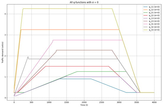
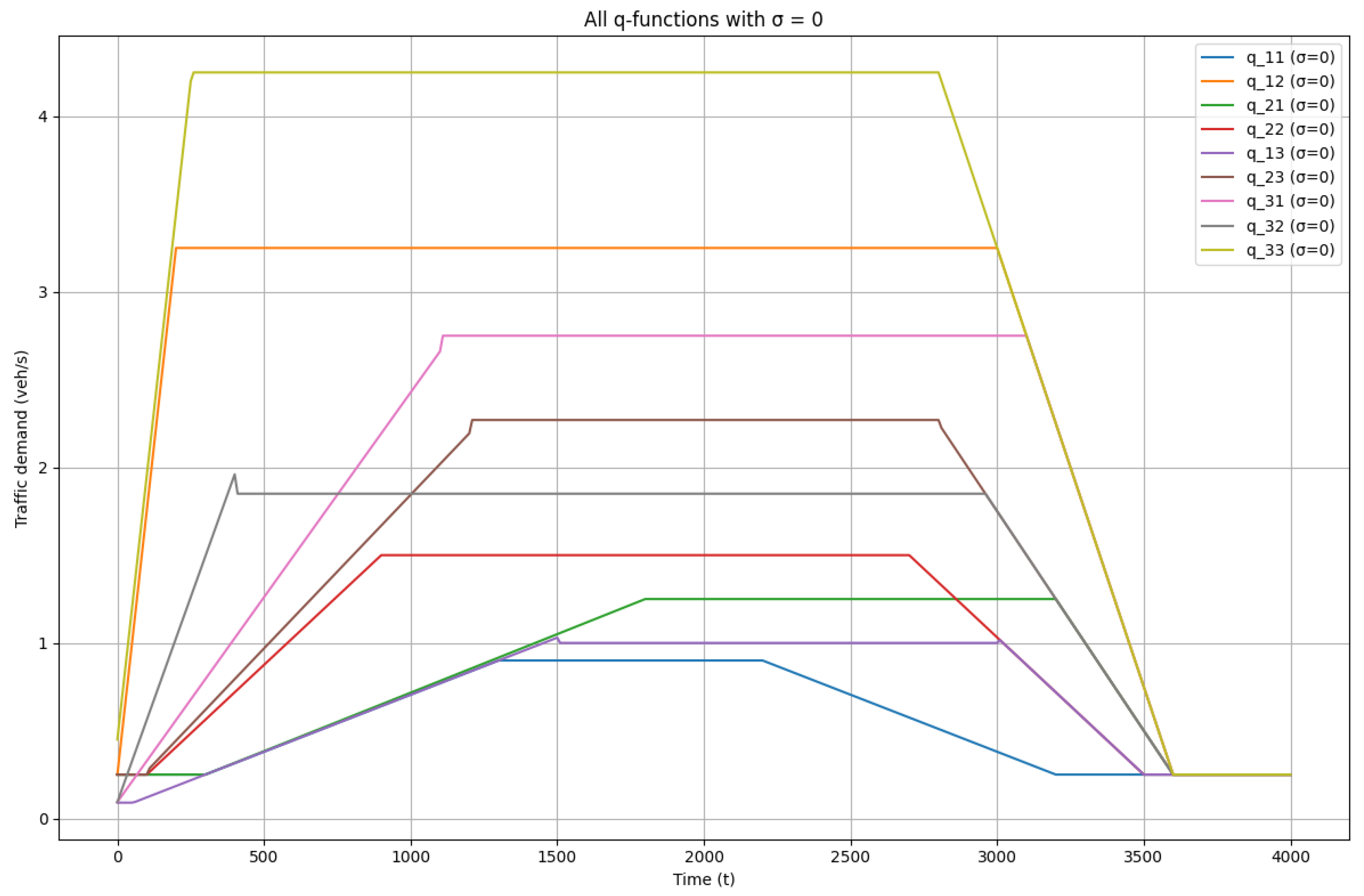
Although the MFD is not derived from a Gaussian model, empirical observations show that its characteristic form often resembles a right-skewed bell shape, with a steep rise under free-flow conditions and a more gradual decline as congestion intensifies. The distribution shows a relationship between the trip completion rate $G_i\left(ni\left(t\right)\right)$ (veh/s) and regional accumulation $n_i\left(t\right)$ and at time step t. In addition, Figure 4 depicts the traffic demand profile $\left(q_{ij}\left(t\right)\right)$, where $i,j=1,2,3$, represents a time-varying inflow of vehicles entering each central region from peripheral neighboring regions. The external inflow serves as the primary disturbance driving increases in network accumulation [24], and is explicitly considered in this work. The evolution is modeled as a piece wise function with time-dependent behavior and stochastic perturbations, specifically defined as

$$q_{ij}(t,\sigma )=max\left(q_{\mathrm{deterministic}}\left(t\right)·(1+ϵ),0\right)·\mathrm{scaler},ϵ\sim \mathcal{N}(0,\sigma )$$

(1)

where

$$q_{\mathrm{deterministic}}\left(t\right)=\left\{\begin{array}{cc}0.25,\hfill & 0\le t\le 100\hfill \\ {\displaystyle \frac{1.25}{800}}t+0.09375,\hfill & 100<t\le 900\hfill \\ 1.5,\hfill & 900<t\le 2700\hfill \\ -{\displaystyle \frac{1.25}{800}}t+5.71875,\hfill & 2700<t\le 3500\hfill \\ 0.25,\hfill & t>3500\hfill \end{array}\right.$$

(2)

Figure 4. Schematic diagram of a three-region traffic demand.

Here, $ϵ$ is a Gaussian random variable with mean zero and standard deviation $\alpha$ capturing inherent stochastic fluctuations in the system. The piecewise segments correspond to distinct operational phases, including initial low-flow, ramp-up, steady high-flow, decline, and final stabilization. The scaler parameter allows for flexible adjustment of the magnitude of $q_{ij}$ for different simulation scenarios. This formulation enables modeling of realistic, time-varying dynamics while incorporating uncertainty, which is critical for accurately simulating [traffic/flow/other domain] behavior in heterogeneous networks. Relying on historical measurements also avoids the noise and uncertainty of real-time estimation or short-term demand forecasting.

3.2. Formulation of MFD Dynamic Equations

The region trip completion $G_i\left(n_i\left(t\right)\right)$ of the MFD is defined as the unrestricted vehicle throughput rate across two or more regions as a function of vehicle accumulation $\left(n_i\left(t\right)\right)$. The expression is formulated in [35] as a third-order polynomial function:

$$G_i\left(n_i\left(t\right)\right)=a_i{n}_i^3\left(t\right)+b_i{n}_i^2\left(t\right)+c_i{n}_i\left(t\right)$$

(3)

where $a_i,b_i,c_i$ are regression parameters. Traffic states are expressed by the transfer accumulations $n_{ij}\left(t\right)$, where $i,j=1,2,3$ are the subregions, implying the number of vehicles originating from $\mathrm{Ri}$ with destinations to $\mathrm{Rj}$, for the time step t. The evolution traffic flow density in the region $\mathrm{Ri}$ follows directly from the mass dynamic vehicle-conservation equations of the MFD system, therefore the i-th region is formulated as follows:

$$n_i\left(t\right)=n_{ii}\left(t\right)+\sum _{j\in N}{n}_{ij}\left(t\right)$$

(4)

The vehicle accumulation $n_{ii}\left(t\right)$ is computed numerically over time by taking the first derivative of Equation (4), expressed as

$${n^{\prime }}_{ii}\left(t\right)=q_{ii}\left(t\right)-M_{iii}\left(t\right)+\sum _{k\in N_i}{M}_{kij}\left(t\right)u_{ki}\left(t\right)$$

(5)

where $M_{kij}$ is the transfer flow trip completion from neighboring region k with destination to region j through the next neighboring region i, while $q_{ij}$ denoting the traffic demand generated in the region i but destined to region j. The transfer trip completion is determined by $u_{ki}$ control variable, while the internal trip completion rate within region i is denoted as $M_{iii}\left(t\right)$ and expressed as follows:

$$M_{iii}\left(t\right)={\displaystyle \frac{n_{ii}\left(t\right)}{n_i\left(t\right)}}{G}_i{n}_i\left(t\right)$$

(6)

where, $n_i=n_{ii}+n_{ij}$ is the addition of vehicle accumulation with origin and destination in region $\mathrm{Ri}$ and those accumulations transitioning in region $\mathrm{Rj}$, applying the same analogy it follows;

$${n^{\prime }}_{ij}\left(t\right)=q_{ij}\left(t\right)+\sum _{k\in N_i}{M}_{kii}\left(t\right)u_{ki}\left(t\right)-\sum _{k\in N_i,k\ne j}{M}_{ikj}\left(t\right)u_{ik}\left(t\right)u_{kj}\left(t\right)-\sum _{i\in N_j}{M}_{ijj}\left(t\right)u_{ij}\left(t\right)\left[j\in N\right]$$

(7)

where $M_{ikj}\left(t\right)$ is the transfer flow from region i through the next immediate region k and with final destination to region j, (i.e., $M_{231}$ is the transfer from region $\mathrm{R}2$, through region $\mathrm{R}3$ with destination to region $\mathrm{R}1$), expressed as

$$M_{ikj}\left(t\right)=p_{ikj}\left(t\right){\displaystyle \frac{n_{ij}\left(t\right)}{n_i\left(t\right)}}{G}_i{n}_i\left(t\right)i\ne j,k\in N_i$$

(8)

where $p_{ikj}\left(t\right)$ is a parameter that defines the route choice and is computed via a Softmax operation, i.e., $p_{ikj}\left(t\right)=exp(-t_{ikj})/{\sum }_{k\in N_i}exp(-t_{ikj})$, where $t_{ikj}$ is the total time taken by vehicle, choosing alternative route (i.e., from region i, through k with destination to region j). The direct vehicle transfer flow from region i with destination region j is further formulated as

$$M_{ijj}\left(t\right)=\left(1-p_{ikj}\left(t\right)\right){\displaystyle \frac{n_{ij}\left(t\right)}{n_i\left(t\right)}}{G}_i{n}_i\left(t\right)i\ne j,k\in N_i$$

(9)

The P-DQN model is designed to control the total network transfer flow across the three regions ($\mathrm{R}1,\mathrm{R}2$ and $\mathrm{R}3$). This is actualized by optimizing perimeter control functions $\left(u_{ij}=u_{12},u_{21},u_{13},u_{31}\right)$. The objective is to maximize the cumulative number of trips completed, equivalently minimizing the total travel time in the traffic system, formulated as follows

$${\mathcal{R}}_t=\underset{u_{ij}\left(t\right)}{max}{\int }_{t_0}^{t_f}\left[M_{122}\left(t\right)+M_{211}\left(t\right)+M_{133}\left(t\right)+M_{311}\left(t\right)\right]dt$$

(10)

where $t_0$ is the start time and $t_f$ is the final time, $M_{122},M_{211},M_{311}$ and $M_{133}$ are transfer flow in and out of the protected region $\mathrm{R}1$, that is from regions $\mathrm{R}2$ and $\mathrm{R}3$, respectively, computed in time steps of t for total period of T expressed in seconds

Subject to:

$$\begin{array}{cc}{n}_{11}^{\prime }\left(t\right)\hfill & =q_{11}\left(t\right)+u_{21}{M}_{211}\left(t\right)+u_{31}{M}_{311}\left(t\right)-M_{111}\left(t\right)\hfill \end{array}$$

(11)

$$\begin{array}{cc}{n}_{12}^{\prime }\left(t\right)\hfill & =q_{12}\left(t\right)+\left[u_{31}{M}_{311}\left(t\right)-u_{12}{M}_{122}\left(t\right)\right]+\left[u_{21}{M}_{211}\left(t\right)-u_{13}{u}_{32}{M}_{132}\left(t\right)\right]\hfill \end{array}$$

(12)

$$\begin{array}{cc}{n}_{13}^{\prime }\left(t\right)\hfill & =q_{13}\left(t\right)-u_{13}{M}_{133}\left(t\right)+u_{21}{M}_{211}\left(t\right)\hfill \end{array}$$

(13)

$$\begin{array}{cc}{n}_{21}^{\prime }\left(t\right)\hfill & =q_{21}\left(t\right)+\left[u_{32}{M}_{322}\left(t\right)-u_{21}{M}_{211}\left(t\right)\right]+\left[u_{12}{M}_{122}\left(t\right)-u_{23}{u}_{31}{M}_{231}\left(t\right)\right]\hfill \end{array}$$

(14)

$$\begin{array}{cc}{n}_{22}^{\prime }\left(t\right)\hfill & =q_{22}\left(t\right)+u_{12}{M}_{122}\left(t\right)+u_{32}{M}_{322}\left(t\right)-M_{222}\left(t\right)\hfill \end{array}$$

(15)

$$\begin{array}{cc}{n}_{23}^{\prime }\left(t\right)\hfill & =q_{23}\left(t\right)-u_{23}{M}_{233}\left(t\right)+u_{12}{M}_{122}\left(t\right)\hfill \end{array}$$

(16)

$$\begin{array}{cc}{n}_{31}^{\prime }\left(t\right)\hfill & =q_{31}\left(t\right)-u_{31}{M}_{311}\left(t\right)+u_{23}{M}_{233}\left(t\right)\hfill \end{array}$$

(17)

$$\begin{array}{cc}{n}_{32}^{\prime }\left(t\right)\hfill & =q_{32}\left(t\right)-u_{32}{M}_{322}\left(t\right)+u_{13}{M}_{133}\left(t\right)\hfill \end{array}$$

(18)

$$\begin{array}{cc}{n}_{33}^{\prime }\left(t\right)\hfill & =q_{33}\left(t\right)+u_{23}{M}_{233}\left(t\right)+u_{13}{M}_{133}\left(t\right)-M_{333}\left(t\right)\hfill \end{array}$$

(19)

The Equations (11)–(19) describe the environmental dynamics, which are internalized by the proposed model but remain unknown in the controller design. The accumulation $n_{11}$ represents the number of vehicles from region $\mathrm{R}1$ with destination in the same region. Similarly, $n_{12}^{\prime }$ is the number of vehicles from region $\mathrm{R}1$ with final destination to region $\mathrm{R}2$, this is implied to all other regions. The total accumulation in Region $\mathrm{R}1$, expressed as $n_1\left(t\right)=n_{11}\left(t\right)+n_{12}\left(t\right)$ (i.e., vehicle originating from region $\mathrm{R}1$ with destination in the same region added to those vehicle transitioning to the region $\mathrm{R}2$), must be maintained below the region’s critical accumulation level. Exceeding this threshold leads to a congestion collapse, significantly degrading traffic flow efficiency. An analogous constraint is imposed on all the regions of the road network ensuring that the aggregate accumulation within every region does not exceed its respective critical limit. In this work, $n_{ii}^{\prime }$ represents the internal accumulation within region i, defined as the sum of the internal traffic demand $q_{ii}$, summation of all incoming controlled transfer flows $M_{kij}$ from neighboring regions, minus the internal completion rate $M_{iii}$ computed numerically. Similarly, $n_{ij}$ denotes the accumulation from region i destined for region j formulated following the same analogy. The vehicle accumulation constraints is given as follows:

$$\begin{array}{c}0\le n_{11}\left(t\right)+n_{12}\left(t\right)\le n_{1,\mathrm{jam}},\hfill \end{array}$$

(20)

$$\begin{array}{c}0\le n_{11}\left(t\right)+n_{13}\left(t\right)\le n_{1,\mathrm{jam}},\hfill \end{array}$$

(21)

$$\begin{array}{c}0\le n_{21}\left(t\right)+n_{22}\left(t\right)\le n_{2,\mathrm{jam}},\hfill \end{array}$$

(22)

$$\begin{array}{c}0\le n_{22}\left(t\right)+n_{23}\left(t\right)\le n_{2,\mathrm{jam}},\hfill \end{array}$$

(23)

$$\begin{array}{c}0\le n_{33}\left(t\right)+n_{32}\left(t\right)\le n_{3,\mathrm{jam}},\hfill \end{array}$$

(24)

$$\begin{array}{c}0\le n_{33}\left(t\right)+n_{31}\left(t\right)\le n_{3,\mathrm{jam}}.\hfill \end{array}$$

(25)

Equations (20)–(25) therefore impose capacity and realism constraints used in the network model. Each inequality enforces physical feasibility for region-level vehicle accumulations at time t. For example, $n_{12}$ defines the number of vehicles in $\mathrm{R}1$ whose destination (or subzone) is $\mathrm{R}2$, while $n_{1,jam}$ is the jam (storage) capacity of region $\mathrm{R}1$. The left-hand part $0\le$ ensures non-negativity, while the right-hand part $\le n_{1,jam}$ limits the summed accumulations in the specified pair of sub-streams so the region never exceeds its maximum capacity storage. The same is implied to all the other regions of the network. The perimeter control constraints are given as $u_{min}\le u_{i,j}\le u_{max}$, where $u_{i,j}\in [0,1]$. The control actions $u_{min}$ and $u_{max}$ define the lower and upper bounds for the variables $u_{12}\left(t\right)$, $u_{21}\left(t\right)$, $u_{13}\left(t\right)$, $u_{32}\left(t\right)$, $u_{23}\left(t\right)$ and $u_{32}\left(t\right)$, computed for time t.

3.3. Formulation of Perimeter Control as Reinforcement Learning Problem

The perimeter traffic control problem is formulated as a Markov Decision Process (MDP), where the RL agent interacts with dynamic MFD states ($n_{ii}$ and $n_{ij}$) and traffic demand states ($q_{ii}$ and $q_{ij}$) to determine optimal control policy actions. The proposed RL framework regulates inter-regional traffic flow by selecting control variables based on the route guidance strategy. It is characterized by a tuple $⟨\mathcal{S},\mathcal{A},\mathcal{R},\pi ⟩$ denoting the state, action, reward, and policy, respectively.

The state, action, reward and policy are defined as follows:

• States $\left(\mathcal{S}\right)$: The states of an MFD-based environment comprises of $n_{ii}$ and $n_{ij}$ vehicle accumulations; additionally, $q_{ii}$ and $q_{ij}$ are traffic demands, averaged over the time step t. Each state element is scaled to [0, 1] through a division by its maximum value factor.
• Action space $\left(\mathcal{A}\right)$: The RL actions are defined by $u_{ij}$ control variables within the admissible $\left[u_{min},u_{max}\right]$ range in addition to direction of route $p_{ikj}$ chosen. Together, these specify a predetermined bound to the extent to which perimeter control values may vary for every time step.
• Reward $\left(\mathcal{R}\right)$: In this paper, the reward is normalized to $[0,1]$ by a large scalar function as suggested in [32]. The agent is trained to maximize the cumulative internal trip completion rate as an objective function stated in Equation (10). Furthermore, a large negative quantity value is added to the reward to penalize unreasonable control strategies that would otherwise result in congestion or invalid accumulations within the time constraint interval.
• Policy $(\pi$): At each time step, the agent chooses an action based on a policy that maps states to actions expressed as

  $$G_t=\sum _t^T{\gamma }^{\tau -1}{\mathcal{R}}_{t+1}$$

  (26)

where $\gamma$ is the discounted rate decaying by $\tau$, T is the total time steps of a single episode, and ${\mathcal{R}}_t$ is reward function expressed in Equation (10). The aim of the P-DQN agent is to optimize the expected value of the return, $\mathbb{E}\left[G_t\right]$, from the start time, which in this work represents the expected total number of trips completed from $t_0$. The perimeter traffic control problem is formulated as an MDP, where an RL agent interacts with MFD and traffic demand states to determine optimal control actions. The state vector comprises regional accumulations and traffic demands, normalized to $[0,1]$. Actions include control variables within predefined bounds, specifying permissible perimeter adjustments per time step. The reward, also normalized, incentivizes cumulative trip completion while penalizing strategies cause congestion. The policy maps states to actions, and is computed by cumulative discounted reward.

3.4. P-DQN Model for Multi-Region Perimeter Control

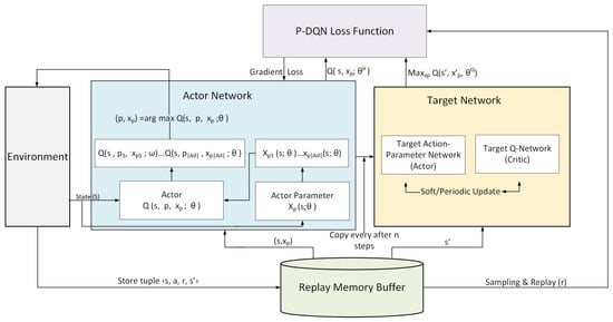
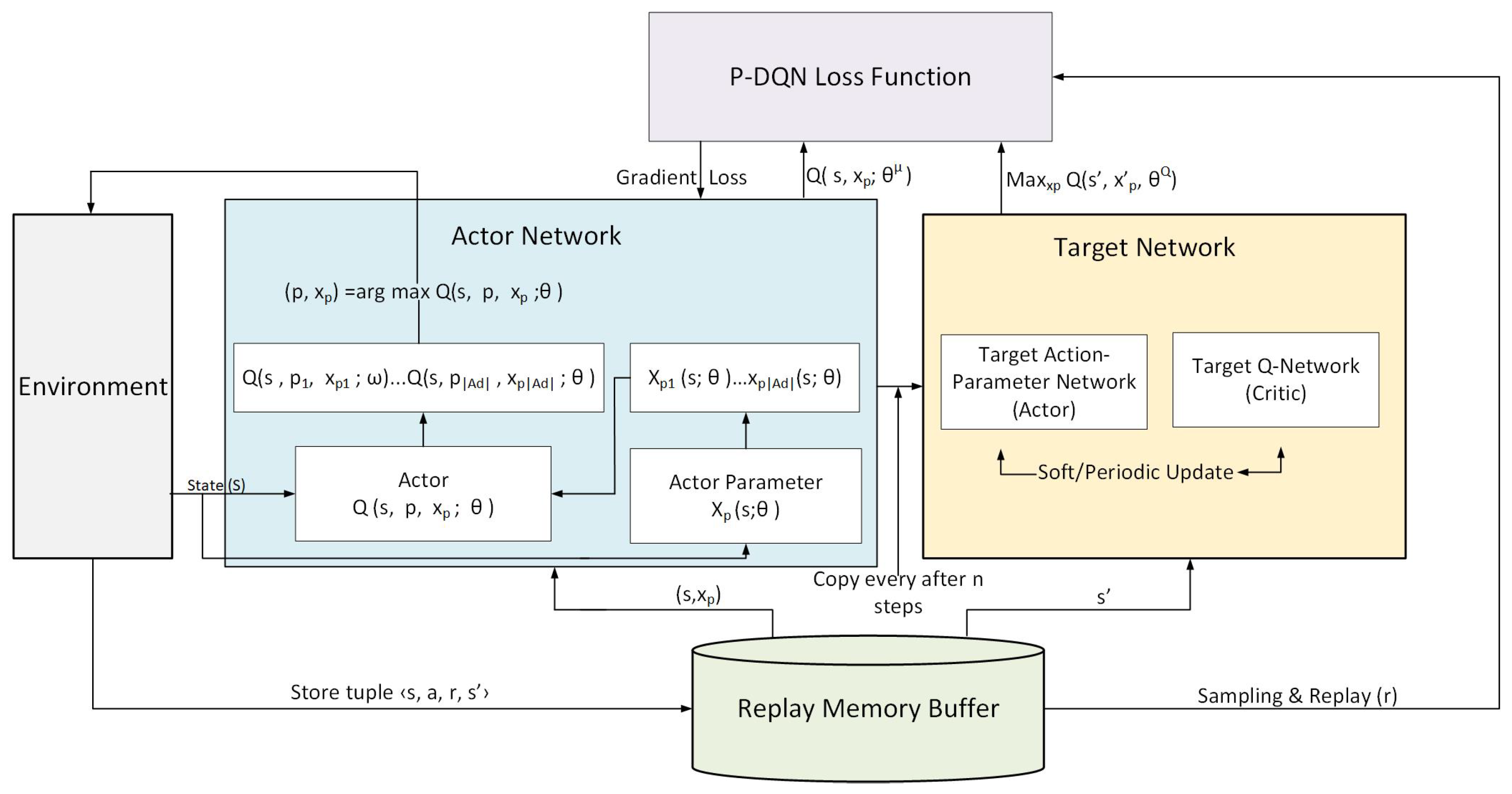
The P-DQN model is designed for control tasks that involve hybrid action spaces composed of discrete decisions and continuous control parameters. The framework employs two neural networks: one approximates the discrete action–value function, while the other generates the continuous parameters that maximize the corresponding Q-value. It further incorporates a replay memory buffer that stores historical transitions and samples randomized mini-batches, which breaks the temporal correlation inherent in sequential traffic data. Together, these mechanisms promote more reliable gradient updates, accelerate convergence, and enhance the overall robustness of the resulting control policy. Figure 5 is an illustration of the networks of P-DQN, which selects the discrete action type by maximizing Q values numerically.

Figure 5. The P-DQNPC training architecture based on P-DQN algorithm.

Let $u_{ij}=x_p\in \mathcal{A}$ denote the action value function, $\left|Ad\right|$ is the discrete action (index) and Q-value function is formulated as $Q(s,a)=Q(s,p_t,x_p)$, the states are given as $s=\left[n_{ij},q_{ij}\right]$. Let $p_t$ be the discrete action given by route choice computed using Softmax algorithm, see Equation (8); it should be noted that $p_t\in p_{ikj}$. Similarly, $x_p$ depicts the associated continuous function for chosen discrete action, in this case control variable is considered in this work as $x_{p_t}\in u_{ij}$. For each discrete action p, the P-DQN model outputs a parameter vector ${\widehat{x}}_p={\mu }_{\theta }(s,p)$ that returns maximum route choice with its associated continuous duration period expressed as

$$p^{\ast }\left(s\right)=\underset{p\in x_p}{argmax}Q(s_{t+1},p^{\prime },\mu (s_{t+1},p^{\prime };{\theta }^{\mu });{\theta }^Q)$$

(27)

where $Q(s,p,x;{\theta }^Q)$ is the critic (value) network and $\mu (s,p;{\theta }^{\mu })$ is the actor (parameter policy) network which returns continuous parameters for the discrete action p, while ${\theta }^{Q\prime }$ and ${\theta }^{\mu \prime }$ are the target networks which are softly updated. Then, the actor network computes action $(p,x_p)=\underset{p,x_p}{argmax}\left(s,p,x_p;{\theta }^{\mu }\right)$; similarly, the Q-function is evaluated by the target network, i.e., the long-term expected cumulative reward for the function $Q(s,x_p)$, expressed as

$$Q(s,x_P)=\mathbb{E}\left[\sum _{k=0}^K{\gamma }^k\mathcal{R}\left(s_{t+k},x_{p_{(t+1)}}|s_t=s,x_{p_{\left(t\right)}}\right)\right]$$

(28)

where $\gamma$ is the discounted factor computed over unit step k. Then, the Bellman target equation used in this work is proposed in [36] as

$$\mathcal{Q}(s_t,p_t,x_{p_t})=\mathbb{E}\left[r_t+\gamma \underset{p\in P}{max}sup{Q}_{(}{s}_{t+1},p,x_p\left)\right|s_t,p_t,x_{p_t}\right]$$

(29)

From the DQN concept, the canonical Bellman target for a sampled transition $Q(s_t,p_t,x_{p_t},s_{t+1})$ is formulated as

$$y_t=\sum _{\tau =0}^{n-1}{r}_t+{\gamma }^n\underset{p\in P}{max}{Q}^{\prime }\left(s_{t+n},p^{\prime },{\mu }^{\prime }\left(s_{t+n},p^{\prime }\right);{\theta }^{Q\prime })\right)$$

(30)

This means that, for each candidate discrete action $p^{\prime }$ at next time step $s_{t+1}$, the actor’s target parameter ${\mu }^{\prime }\left(s_{t+1,p^{\prime }}\right)$ is evaluated with the target critic $Q^{\prime }$ to enable the actor network to choose optimal $p^{\prime }$. The objective is for the actor parameters ${\theta }^{\mu }$ to compute parameters $x_p$ that increase the function Q value; this is expressed in [37,38] as

$$J\left(\theta \right)={\mathbb{E}}_{s\sim \mathcal{D},p\sim disct}\left[Q\left(s,p;{\theta }^{\mu }(s,p)\right)\right]$$

(31)

For the sampled discrete action $p_t$, the actor gradient (deterministic) is expressed follows:

$${\nabla }_{{\theta }^{\mu }}\left(J\right)\approx \mathbb{E}\left[{\nabla }_{x_{p_t}}Q\left(s_t,p_t,x_{p_t};{\theta }^Q\right).{\nabla }_{{\theta }^{\mu }}\mu \left(s_t,p_t;{\theta }^{\mu }\right)\right]$$

(32)

where $x_{p_t}=\mu \left(s_t,p_t;{\theta }^{\mu }\right)$ and a gradient ascent step is numerically computed, i.e., ${\theta }^{\mu }\leftarrow {\theta }^{\mu }+{\beta }_{\mu }{\nabla }_{{\theta }^{\mu }}J$. For any chosen target $y_t$, the Temporal Difference (TD) error (critic loss) is given as

$${\mathcal{L}}_Q={\mathbb{E}}_{s,p,x,r,s^{\prime }}\left[{\left(y_t-Q(s,p,x_p|{\theta }^Q)\right)}^2\right]$$

(33)

In a similar manner, the objective of actor network is to minimize policy loss function; this is designed to maximize the Q-value for the chosen discrete action and its parameters using gradient decent; expressed as

$${\mathcal{L}}_{\mu }=-{\mathbb{E}}_{\sim \mathcal{D}}\left[Q\left(s,p,{\pi }_x\left(s,p^{\ast }|{\theta }^{\mu }\right)|{\theta }^Q\right)\right]$$

(34)

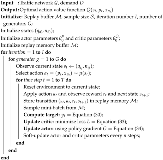
The P-DQN algorithm improves learning stability by employing both actor network and a target network that provides fixed Q-value estimates during temporal-difference updates. The actor and target networks are trained using gradient descent to minimize a loss function that captures the difference between predicted and target Q-values; this is done by updating network parameters iteratively. P-DQN learns an optimal policy to regulate inter-regional traffic flow, maximizing cumulative discounted rewards while addressing scalability and hybrid-action limitations of conventional RL approaches. The P-DQN pseudocode is illustrated in Algorithm 1.   

Algorithm 1: Proposed P-DQN learning algorithm.

4. Experimental Setup

This section describes the setup and configuration used to evaluate the performance of the proposed perimeter control strategies. The experiments are designed to provide a controlled environment for systematic analysis as well as realistic conditions to assess practical applicability. The study is divided into two parts: one based on synthetic MFD data, which allows precise control over network demand and traffic dynamics, and the other based on real-world PeMS traffic data, which captures the stochastic and complex nature of actual urban traffic. The pseudocode for P-DQNPC scheme is are formalized in Algorithm 1. The list of important hyperparameters for the P-DQN agents is presented in Table 2.

Table 2. P-DQN hyperparameters and python packages used in this work.

Hyperparameters	P-DQN Value	Description
Actor epochs	5	Times gradient descent is computed for the actor network
Actor learning rate	0.0025	Learning rate for actor network updates
Actor learning rate decay	0.95	Exponential decay factor for actor learning rate
Action range	0.1–0.9	Continuous action space limits
Batch size	128	Number of transitions per network update
Critic epochs	64	Forward and backward passes for critic training
Critic learning rate	0.001	Initial Adam optimizer learning rate for critic network
Critic learning rate decay	0.01	Exponential decay factor for critic learning rate
Discount factor ($\gamma$)	0.95	Used to calculate the learning targets
Discrete action space	1, 2, 3	Represents the three cluster regions in the network
Early stopping patience	10	Number of epochs with no improvement before stopping training
Training time	3600 s	Total time for full iterations (60 s per step)
Generator (G)	6	Number of generators collecting learning experiences
Iteration (I)	125	Total number of rounds to train the agents
Noise parameter ($\sigma$)	0.2	Exploration decay per iteration
Replay memory ($\mathcal{M}$)	10,000	Replay buffer capacity
Sample size ($\mathcal{S}$)	1000	Number of samples per network update
Sigma and alpha ($\sigma ,\alpha$)	0.2, 0.2	High uncertainty in traffic demands and MFDs
Python Packages/Components
Keras	2.13.1	Deep learning library used to build actor and critic networks (with TensorFlow 2.15.0 backend)
Adam Optimizer	Included in Keras 2.13.1	Adaptive learning rate optimizer for network training
64 Dense Layers	N/A	Fully connected layers in the network (64 neurons each)
ReLU Activation	N/A	Nonlinear activation function for hidden layers
Kernel Initializer	N/A	Method to initialize network weights for proper convergence
Pandas	2.1.0	Data handling and preprocessing library
NumPy	1.26.0	Numerical computations and array operations
Matplotlib	3.8.0	Plotting library for visualizing results

4.1. Experimental Setup for Synthetic MFD Data

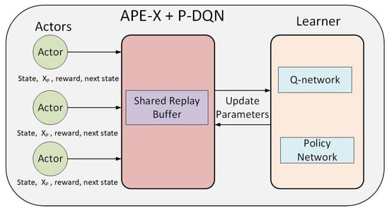
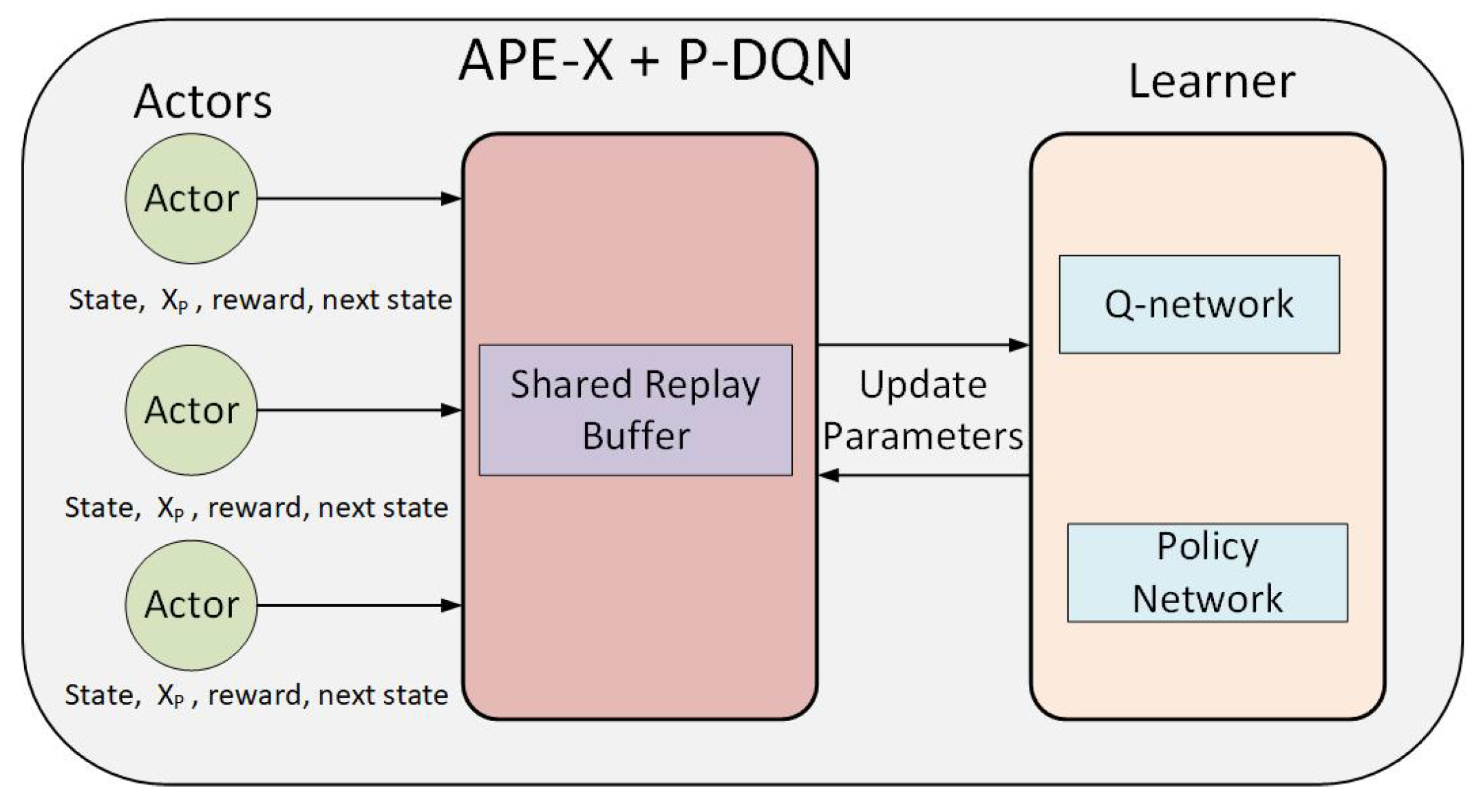
The P-DQN agents require extensive interaction data, motivating the use of the Ape-X distributed framework [39] for large-scale parallel experience generation. As shown in Figure 6, multiple actors interact with independent environment instances under diverse exploration strategies, while a centralized learner updates network parameters using a shared prioritized replay buffer.

Figure 6. Overview of the Ape-X distributed P-DQN action architecture.

Updated parameters are periodically synchronized across all actors, enabling stable and efficient distributed training. In this process, higher priority is assigned to experiences reflecting more informed agent decisions, while obsolete samples are removed once the replay buffer reaches capacity. The centralized learner uniformly samples from the buffer and employs these experiences to update the agents’ neural network parameters. For the three-region network considered in this work, the MFD for $\mathrm{R}3$ is the same as the one observed in [40], whereas a scaled-down versions of it is adapted for $\mathrm{R}2$ and $\mathrm{R}1$ as illustrated in in Figure 3, which exhibits higher demand to $\mathrm{R}1$ than to $\mathrm{R}2$ and $\mathrm{R}3$ (the periphery of a city) during the 1-hour period. The critical accumulation values for the experiments are selected based on the maximum productivity points of each region’s MFD set as follows; $n_{1,crt}=3290$ veh, $n_{2,crt}=6200$ veh and $n_{3,crt}=8200$ veh, respectively. These values reflect the peak traffic throughput for each region, ensuring that the simulations test the P-DQN framework under near-capacity conditions and provide realistic validation of its ability to prevent congestion while maximizing trip completion. This approach ensures that the simulation results are both physically meaningful and representative of real-world urban traffic dynamics. The state variables and rewards are scaled in the range of [0, 1] to ensure numerical stability. The initial traffic states in R1 and R2 are, respectively, assumed to be uncongested with $n_1\left(t0\right)=2500$ veh and $n_2\left(t0\right)=3000$ veh and $n_3\left(t0\right)=5000$ veh, respectively, considered arbitrarily. Specifically, the MFDs and traffic demands in the environment are expressed in [18] as follows

$${\widehat{g}}_i\left(n_i\left(t\right)\right)=g\left(n_i\left(t\right)\right)+\beta \left(t\right).n_i\left(t\right),i=1,2,3$$

(35)

$${\widehat{q}}_{ij}\left(t\right)=max(q_{ii}\left(t\right).\left(1+\chi \left(t\right)\right),0),i,j=1,2,3$$

(36)

where $\beta \left(t\right)$∽$U(-\alpha ,\alpha )$ and $\chi \left(t\right)$∽$N(0,{\sigma }^2)$. It should be noted that $\alpha$ and $\sigma$ are levels of uncertainty in the MFDs and traffic demands, respectively. As regional traffic congestion increases, the deviation between predicted and actual trip completion rates also grows, aligning with both empirical and analytical evidence found in the papers [41]. Another study in [42] shared mobility probe data to analyze how travel time reliability breaks down under real congestion, showing that as demand and traffic pressures increase, variability and unreliability grow effectively demonstrating empirical patterns of predicted against actual travel time performance.

4.2. Experimental Set Up for Real World Data (PeMS Data)

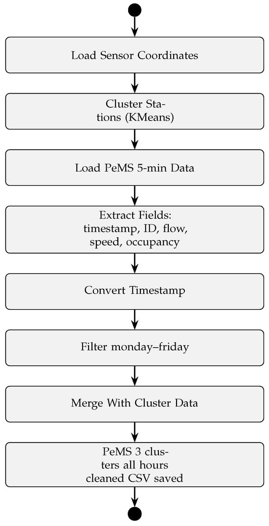
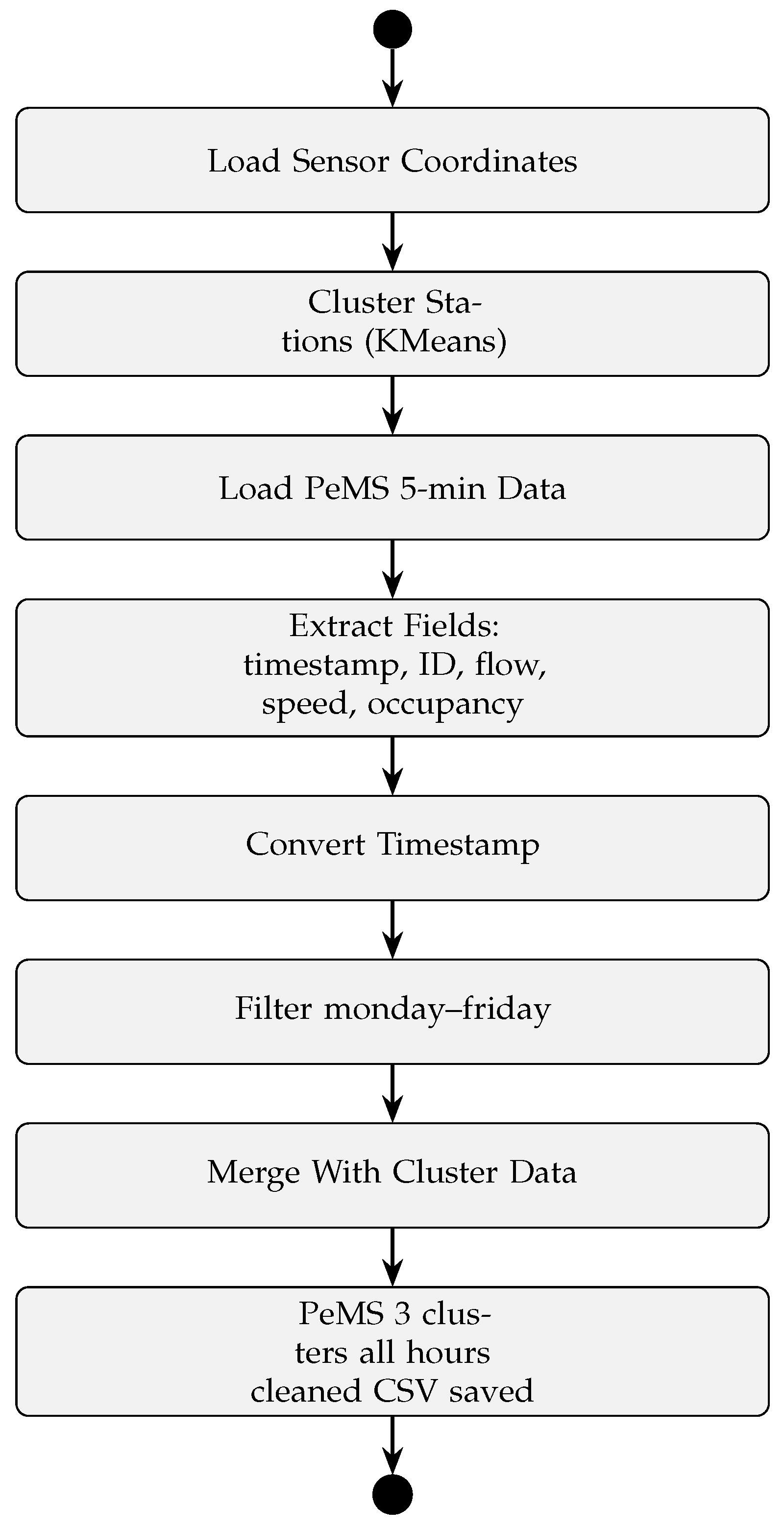
Figure 7 shows the workflow chart for PeMS traffic data processing, including station clustering, field extraction, timestamp conversion, full-day filtering, region merging, and saving the cleaned dataset in CSV file for reinforcement learning analysis.

Figure 7. PeMS traffic cluster dataset preprocessing flow chart. Available online: (https://pems.dot.ca.gov) (accessed on 24 October 2025).

The choice of PeMS traffic data is motivated by its high spatial and spatiotemporal resolution, extensive coverage, and accessibility, making it one of the most comprehensive traffic datasets worldwide and free access. PeMS provides real-time measurements from thousands of loop detectors across California highways, capturing diverse traffic conditions, sensor identification using position latitudes and longitudes which allows for regional clustering, vehicle speed, flow rate and vehicle positioning in real time. Using this dataset allows the proposed P-DQN framework to be trained and validated under realistic, large-scale traffic state environments, ensuring that the derived models are robust and applicable to real-world networks. By leveraging this dataset, the framework can replicate traffic management challenges prevalent in other cities, including multi-region congestion, high variability in demand, and the need for coordinated perimeter control. Consequently, the insights and performance of the P-DQN model validated on PeMS can be generalized and adapted to other urban networks worldwide, supporting its broader applicability in intelligent traffic management systems.

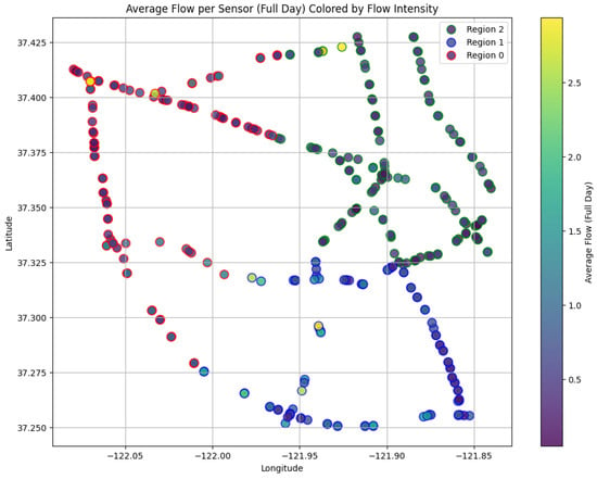
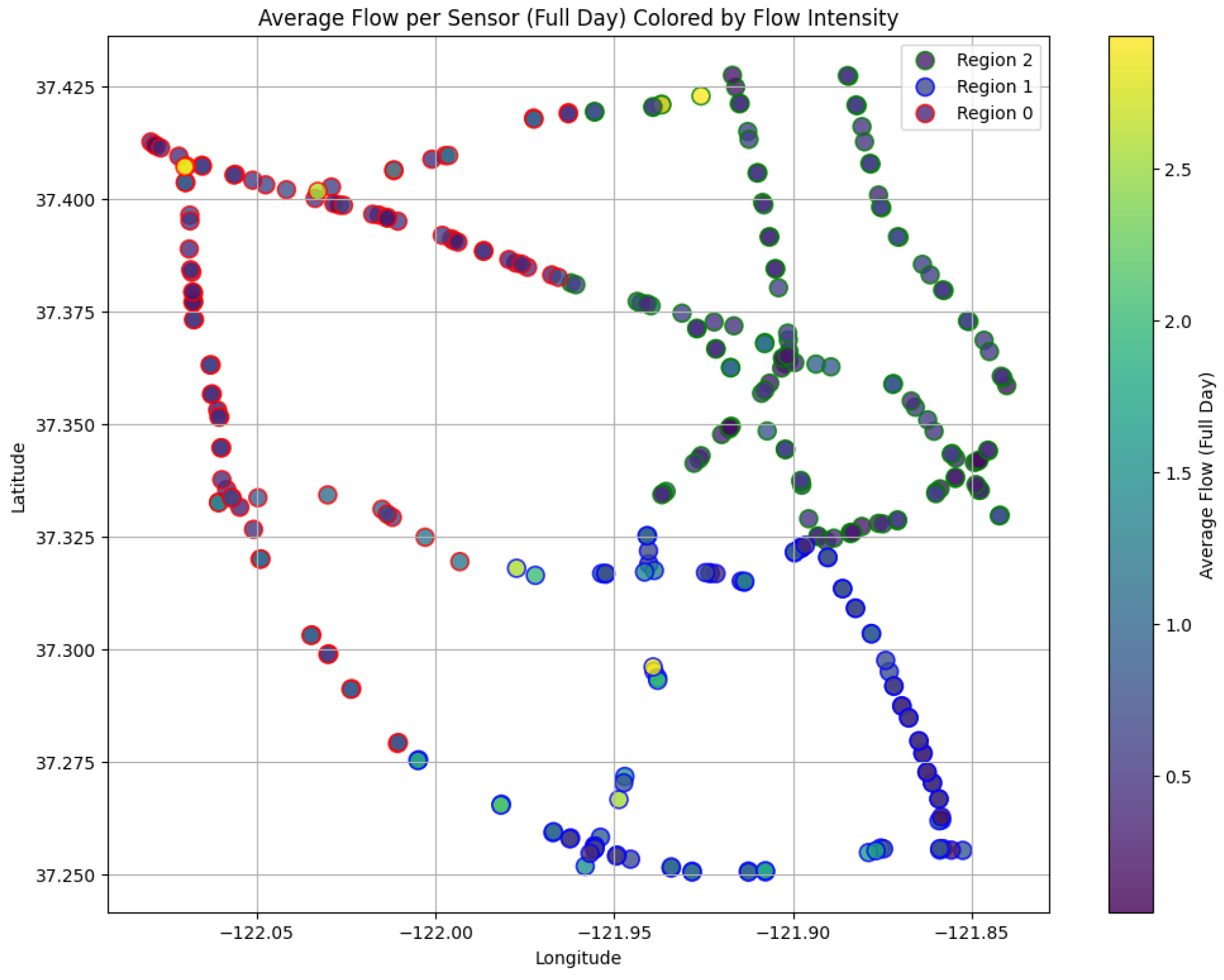
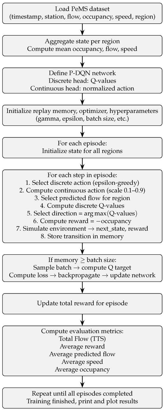
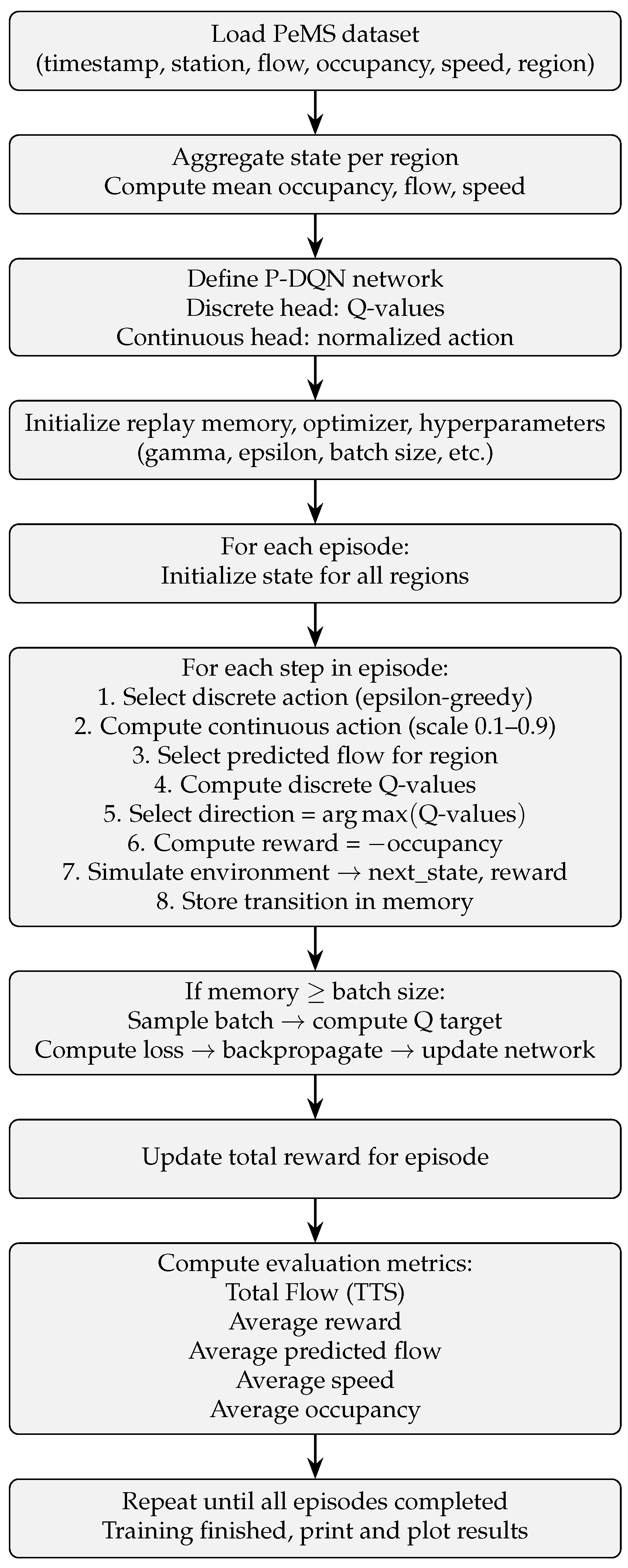
Figure 8 presents a spatial distribution of traffic sensors, where each point denotes a sensor location colored according to its average flow measured between 7:00 a.m. and 5:00 p.m.. Sensors are grouped by their assigned regions, enabling a visual comparison of flow patterns across the network. Darker red markers indicate sensors operating under higher flow conditions, whereas lighter tones represent lower demand. The plot highlights spatial variations in congestion and identifies heavily loaded zones that are critical for evaluating network performance and guiding perimeter-control strategies. Figure 9, present flowcharts for the P-DQN perimeter control framework. The training diagram outlines regional state aggregation, hybrid action selection, environment interaction, replay-memory updates, and batch-based neural network training with episode-level reward accumulation. The evaluation diagram depicts the application of the trained P-DQN model to multi-region traffic data, including data preprocessing, state construction, actor–critic action generation, reward computation, and performance assessment using throughput, average reward, vehicle flow, speed, and occupancy metrics.

Figure 8. Spatial grouping by region.

Figure 9. P-DQN perimeter control algorithm.

5. Experimental Results and Findings

This section presents the performance evaluation of the proposed perimeter control strategies under different experimental settings. The results are organized into two parts to highlight the effectiveness and robustness of the control approaches under both controlled and realistic scenarios. In the first part, synthetic experiments using MFD data are analyzed, which allows for systematic examination of the network-level traffic dynamics under well-defined conditions. In the second part, an evaluation of RL-based controllers using real-world traffic measurements from the PeMS dataset, which captures complex and stochastic traffic patterns observed in the California highway network. The data used in this study are obtained from the source documented in [43]. These experiments provide complementary insights into the performance, stability, and robustness of the proposed reinforcement learning-based methods under both idealized and practical traffic conditions.

5.1. Experimental Results for Synthetic MFD Data

In this work, the performance metric curves of the P-DQN perimeter control model is compared to No-Control (NC) and DDPG schemes as baselines under high uncertainty in traffic demands and MFDs configurations, while the simulations were carried out for all three regions ($\mathrm{R}1$, $\mathrm{R}2$, and $\mathrm{R}3$) to capture the full dynamics of the network, the performance metric curves reported in this study focus on regions $\mathrm{R}1$ and $\mathrm{R}2$. This choice is motivated by the need for a direct and meaningful comparison with previous studies, which predominantly considered only two regions. By limiting the comparison metrics to $\mathrm{R}1$ and $\mathrm{R}2$, this work maintain consistency with prior benchmarks, while still leveraging the richer three-region simulation to assess the generalization and robustness of the proposed P-DQN scheme. This approach ensures that improvements demonstrated in the reported metrics reflect true performance gains relative to existing methods, without introducing inconsistencies due to differing network sizes. Perimeter control aims to improve network productivity, measured by cumulative trip completion (CTC), or equivalently, to minimize total travel time (TTT). The CTC and TTT serve as the primary metrics for evaluating the three control strategies, which are tested across deterministic traffic environment and high-uncertainty traffic and MFD scenarios.

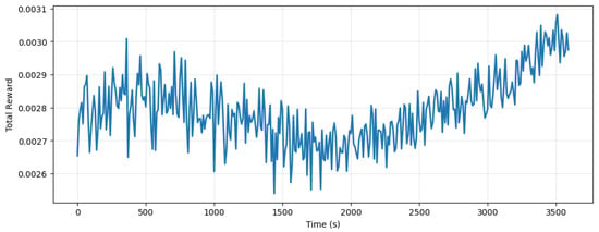
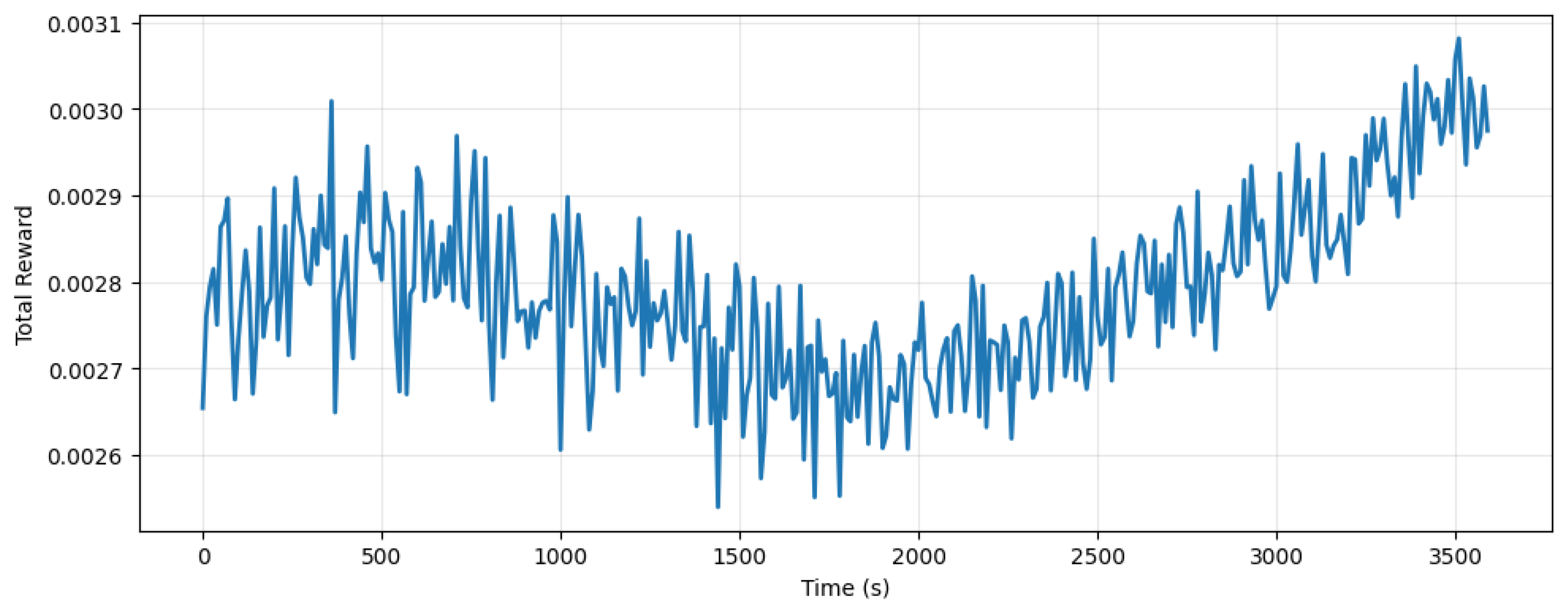
Figure 10 illustrates the temporal progression of the P-DQN agent’s reward signal during training and continuous perimeter-control actions. During the initial training period (0–200 s), the model exhibits a stronger bias toward exploration than exploitation. After that the model increasingly exploits the learned policy, leading to a steady upward trend in the reward and indicating improved policy performance. This shows that the learned control actions increasingly align with the system objective of stabilizing regional traffic conditions and enhancing network throughput.

Figure 10. P-DQN total reward over step time.

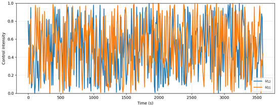
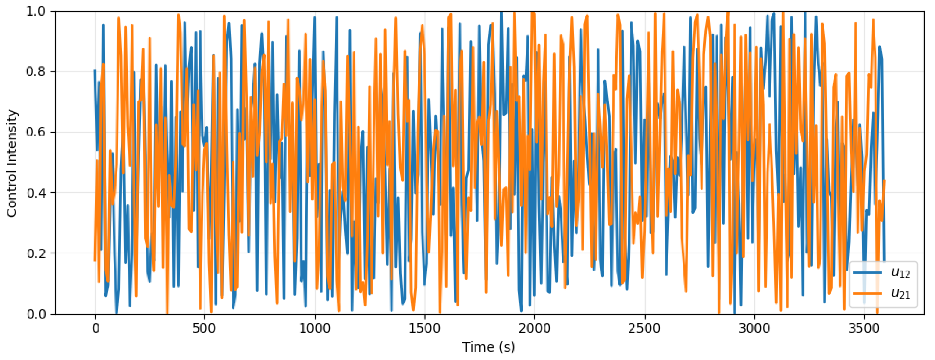
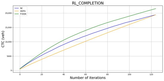
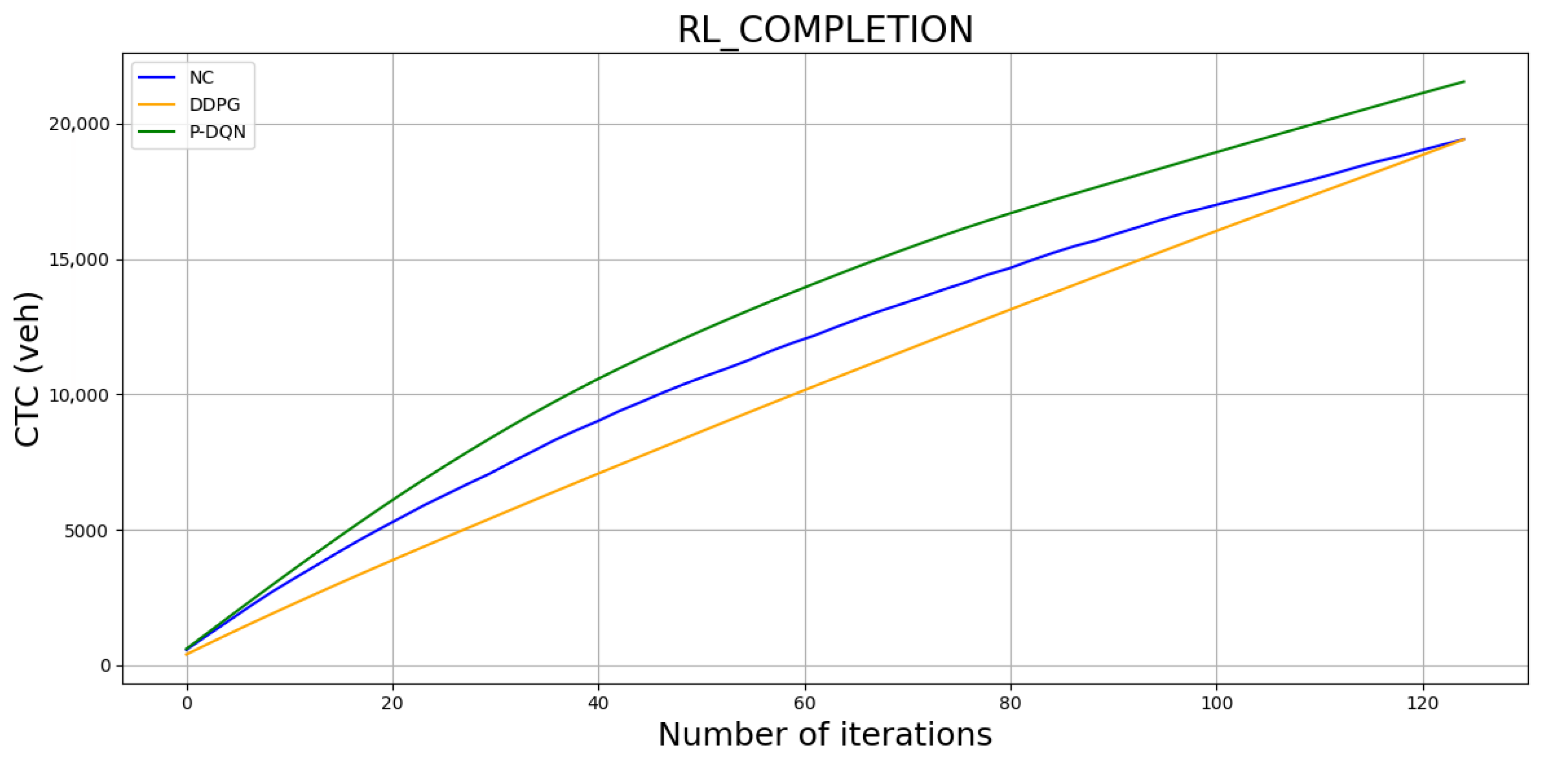
Figure 11 shows time-varying continuous control inputs generated by the P-DQN agent which regulates inter-regional flows. In the P-DQN framework, the control action $u_{21}$ regulates traffic moving from region $\mathrm{R}1$ to region $\mathrm{R}2$, while $u_{12}$ governs traffic in the opposite direction. Both controls adapt dynamically to changing congestion levels, the actions are independent of each other and are presented on same frame for comparison purposes. The continuous-control plot indicates that $u_{21}$ is more consistently aligned with the reward function, demonstrating tighter regulation of traffic flow compared to $u_{12}$. The trajectories highlight the controller’s ability to modulate transfer flows in response to network traffic demand and accumulation variations. Figure 12 displays the evolution of accumulative trip completion (CTC) across consecutive training episodes. The model is trained in high uncertainty in MFD and traffic demand with similar results for deterministic environments. It is observed that P-DQN agent achieved the best performance for first 120 iterations by allowing the highest number of vehicle to across the two regions $\mathrm{R}1$ and $\mathrm{R}2$.

Figure 11. P-DQN continuous action over step time.

Figure 12. Total evolution of accumulative trip completion.

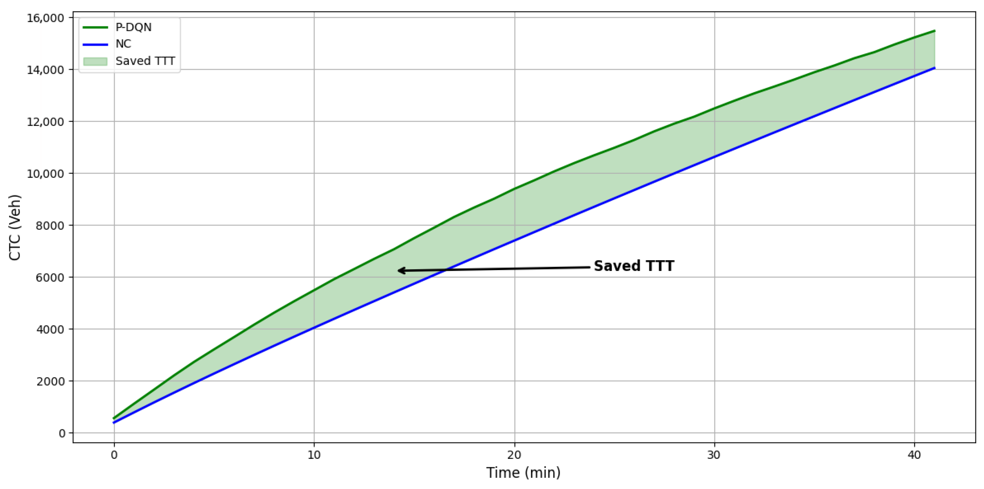
The plots show that the P-DQN scheme consistently outperforms both NC and DDPG. This improvement is largely attributed to its hybrid action structure, which combines discrete and continuous control, enabling more effective decision making in high-dimensional traffic environments. Although NC performs better than DDPG, the latter struggles because it requires substantially more training and has difficulty learning good attributes from the large, complex traffic state space, resulting in poorer overall performance. Figure 13 demonstrates that the P-DQN approach exhibits strong potential for MFD-based network traffic control. Overall, the results indicate that reinforcement-learning-based perimeter control strategies can effectively reduce congestion across the network. The P-DQN algorithm achieved trip completions significantly more efficiently than the NC strategy, creating a substantial area between their completion curves, which corresponds to the TTT saved. From the plotted results, the average throughput of P-DQN is 8997 veh, compared to 7450 veh for NC, representing 20.8% improvement. This highlights the clear advantage of perimeter control over the NC approach.

Figure 13. Evolution of trip completion over time for the P-DQN against NC control and saved TTT.

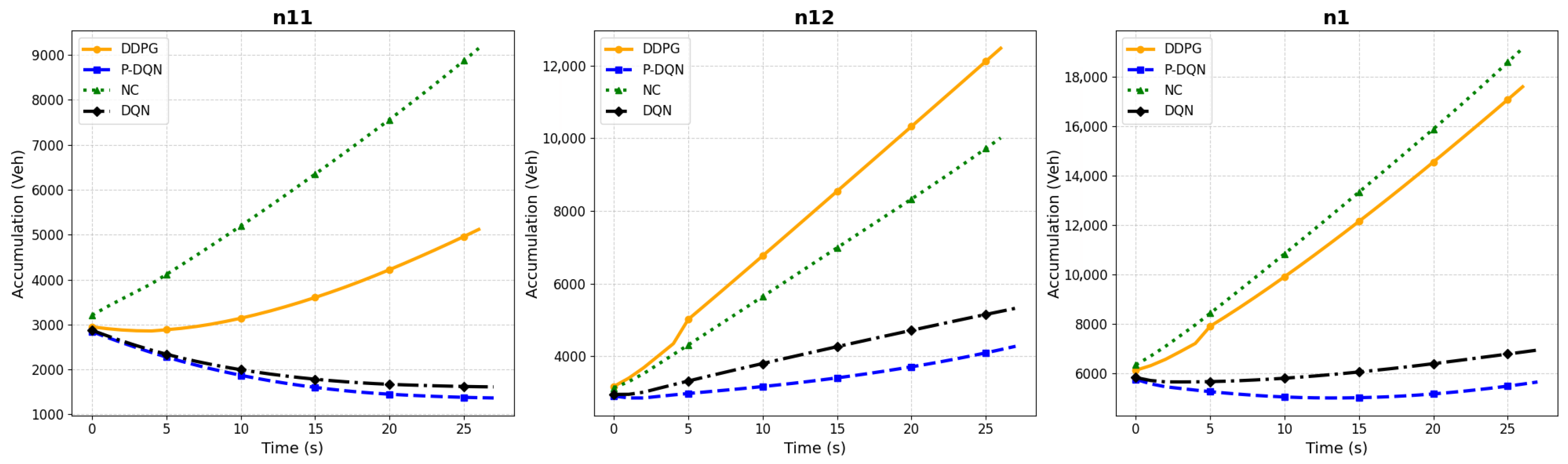
Figure 14 depicts the evolution of accumulation as applied a deterministic scenario for both traffic demand and MFDs ($\sigma =0,\alpha =0$) as a benchmark see Equations (35) and (36). The vehicle accumulation in region $\mathrm{R}1$, defined by $n_1=n_{11}+n_{12}$, where $n_{11}$ denotes vehicles originating in $\mathrm{R}1$ with destinations within same region and $n_{12}$ represents vehicles transitioning to the next region $\mathrm{R}2$. The P-DQN controller consistently maintains the lowest accumulation levels for both internal and transferring traffic, remaining well below the critical threshold of approximately 4000 veh.

Figure 14. Evolution of accumulations in deterministic traffic demands and MFD for region $\mathrm{R}1$.

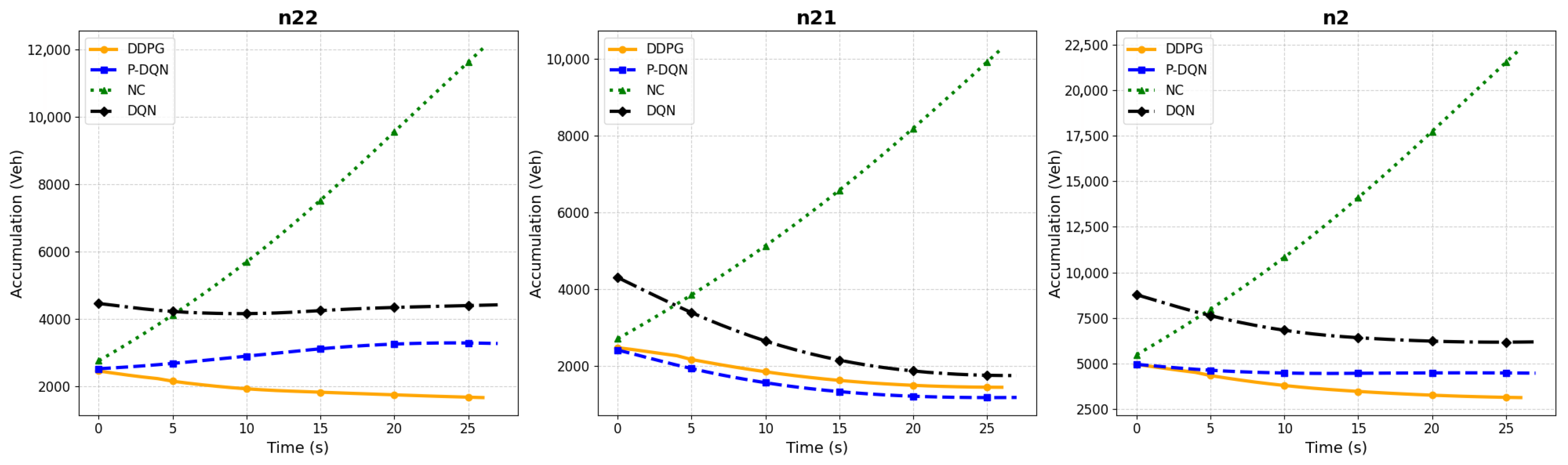
This behavior indicates smooth and stable flow conditions throughout the simulation horizon. In contrast, DQN, DDPG and NC exhibit rapid accumulation growth, saturating within the first 5 min and resulting in severe traffic congestion. Figure 15, shows the vehicle accumulations (i.e., $n_2=n_{21}+n_{22}$) from region $\mathrm{R}2$ with destination in the same region or transitioning to region $\mathrm{R}1$ for a period of 25 min. It is observed that, when $u_{21}$ perimeter control is applied, just a fraction of vehicles are transferred to $\mathrm{R}1$, while the rest instead remains within $\mathrm{R}2$. In this scenario, the P-DQN model is able to transfer the blocked traffic through neighboring region $\mathrm{R}3$, thus maintaining the lowest accumulation $n_{21}$ to reach region $\mathrm{R}1$. From the plot, the P-DQN curve consistently trends below the DQN, DDPG and NC plots, indicating that P-DQN is able to extract better control actions (route selection and time duration) that reduce delays and resolve congestion more effectively.

Figure 15. Evolution of vehicle accumulations in the deterministic environment from region $\mathrm{R}2$.

The smoother and generally lower trajectory of the P-DQN scheme suggests more stable learning and improved decision making at both low and high-traffic loads. This makes the performance of our model superior to DDPG and NC with a steady and lower congestion below critical accumulation of 6200 veh. It should noted that NC quickly saturates, causing severe congestion.

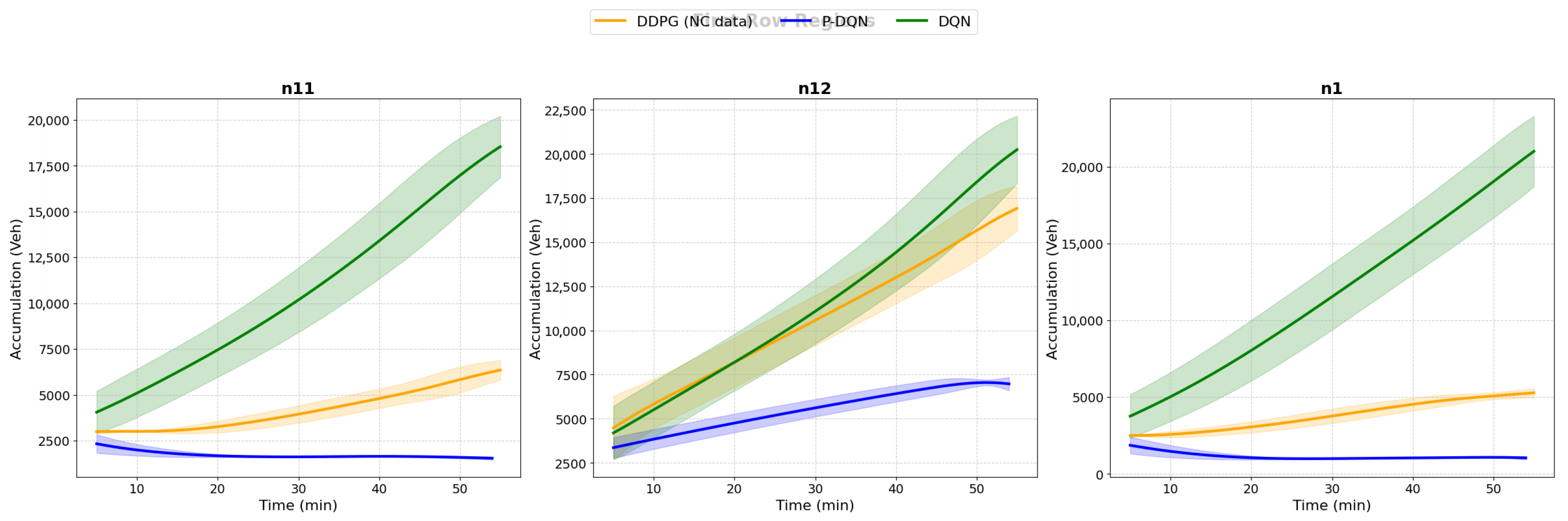
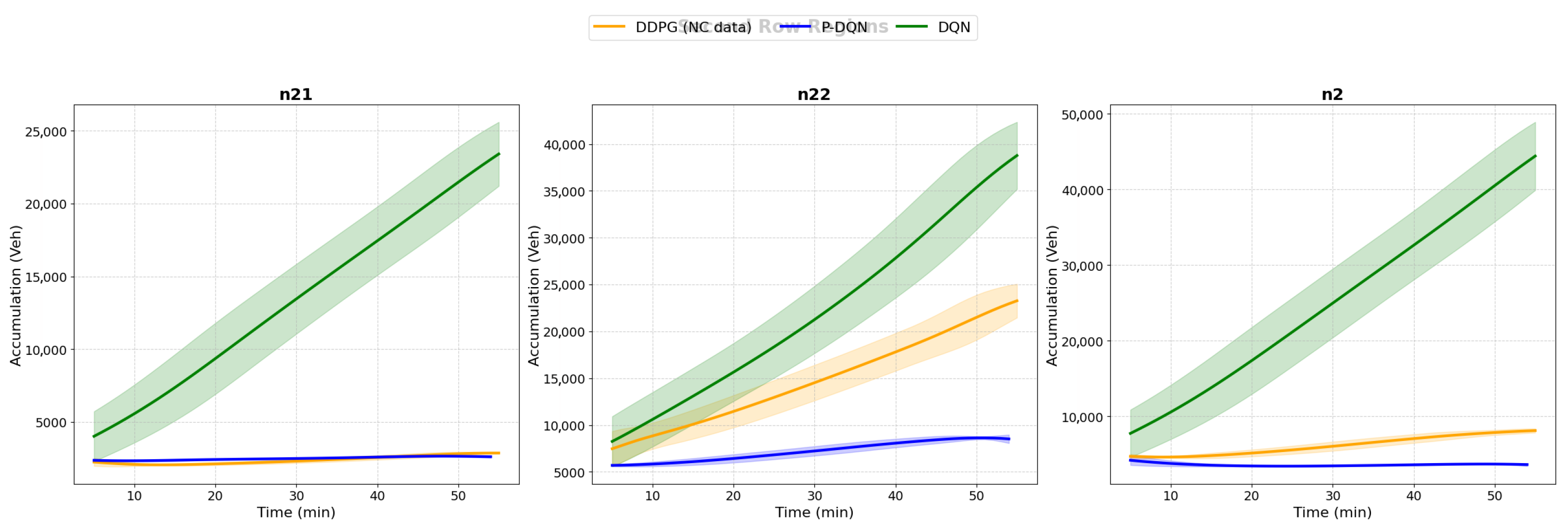
The comparative subplots with 95% confidence intervals in a high uncertainty in traffic demand and MFDs scenarios (i.e., $\sigma =0.2,\alpha =0.2$) are displayed in Figure 16 for vehicle accumulations in region $\mathrm{R}1$ and Figure 17 for region $\mathrm{R}2$ respectively. Figure 16 illustrates the comparative performance of the P-DQN, DDPG, and NC control strategies for traffic management in region $\mathrm{R}1$. The evaluation is conducted based on vehicle accumulations, namely $n_{11}$, $n_{12}$, and the total accumulation $n_1$. From the subplots it is noted that P-DQN.

Figure 16. Evolution accumulations in high-uncertainty traffic demand and MFDs for regions $\mathrm{R}1$.

Figure 17. Evolution accumulations in high-uncertainty traffic demand and MFDs for regions $\mathrm{R}2$.

Algorithm consistently achieves the lowest mean accumulation of below 5000 veh with narrow confidence intervals, demonstrating both effective congestion mitigation and high stability under stochastic traffic demand. In contrast, DQN, DDPG exhibits higher mean accumulation and wider confidence intervals, indicating sensitivity to state-space complexity and less reliable performance, Additionally, NC shows the highest accumulation with moderate-to-wide intervals. Reflecting predictable but suboptimal uncontrolled behavior.

Figure 17, shows vehicle accumulations ($n_{21},n_{22},n_2$) subplots for region $\mathrm{R}2$ under high traffic demand and MFD uncertainty. Both P-DQN and DDPG displays similar vehicle accumulations of lower than 2500 veh transfer accumulation from region $\mathrm{R}2$ towards region $\mathrm{R}1$ (i.e., $n_{21}$). However, it should be noted that P-DQN outperforms DDPG and NC for internal vehicle accumulation $\left(n_{22}\right)$ with less than 7000 veh against unprecedented vehicle upsurge for the other two algorithms. Similarly, P-DQN displays much lower total region accumulation $\left(n_2\right)$ against DDPG and NC schemes. The obtained results demonstrate that the proposed P-DQN framework significantly enhances traffic signal control efficiency while maintaining low congestion levels. Moreover, the method exhibits robust and stable performance across varying uncertainty realizations within dynamic traffic environments.

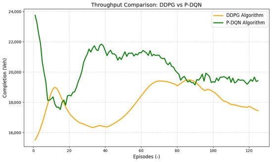
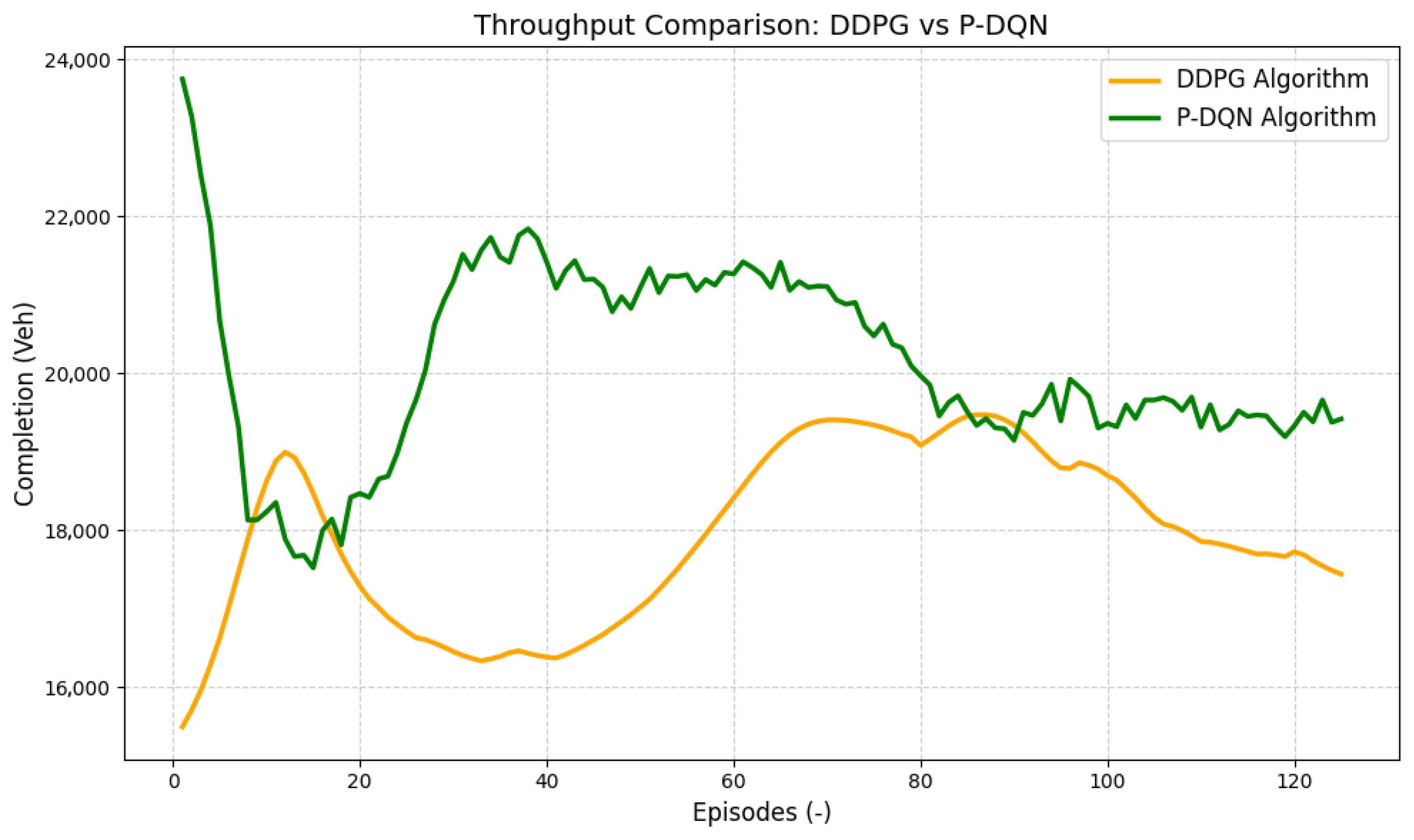
Unlike MFDRLPC [12], which employed two separate RL agents, DQN for discrete actions and DDPG for continuous actions. P-DQN integrates both discrete and continuous action selection within a single parameterized with Ape-X distributed framework. As detailed in the algorithm and implemented in our Python code, the discrete gating decision and the corresponding continuous flow control are jointly optimized by a single agent, enabling coordinated decision making and more efficient policy learning. This integration distinguishes P-DQN from MFDRLPC, reducing redundancy and improving scalability across multiple regions, while maintaining the flexibility to adapt both discrete and continuous control in real time. Figure 18 shows the vehicle throughput rate per episode, the plots comparison are reinforced by the numerical analysis: computing the mean throughput for each algorithm shows that P-DQN achieved a higher average number of completed vehicles, resulting in an approximate performance gain of 12.26%.

Figure 18. Comparison of total trip completion rate for P-DQN and DDPG algorithms.

The P-DQN curves consistently trend above the DDPG curve, indicating that P-DQN is able to extract better control actions that reduce delays and resolve congestion more effectively. The smoother and generally higher trajectory of the P-DQN line suggests more stable learning and improved decision making at both low and high traffic loads. Conversely, the DDPG curve shows higher fluctuations and overall lower completion values, reflecting greater sensitivity to state transitions and less robust convergence. The difference in area between the two lines reflects the cumulative impact of policy quality over the full episode horizon. This confirms that the parametric action representation in P-DQN enables the agent to handle discrete–continuous traffic control more efficiently than the fully continuous exploration of DDPG algorithm.

5.2. Comparison with State-of-the-Art Methods

In this subsection, the performance of the proposed P-DQN for multi-region traffic control against a recent state-of-the-art (SOTA) method, Graph-MAPPO is evaluated. The goal is to provide a rigorous benchmark demonstrating the effectiveness of P-DQN in controlling vehicle flows and reducing congestion across interconnected regions. We describe the two-region traffic environment, outline the training parameters for both agents, and present quantitative results including cumulative rewards, average queue lengths, confidence intervals, and statistical tests. The comparison highlights the advantages of P-DQN over Graph-MAPPO in terms of reward maximization and congestion mitigation, addressing the reviewer’s concern about the omission of recent SOTA methods. Experimental setup and confidence interval and statistical results is shown in Table 3.

Table 3. Experimental setup parameters and performance statistics for two-region traffic control.

Component/Metric	Description/Value
Environment	Two-region traffic network with stochastic arrivals, queues, and flows; observations per region: vehicle count, queue length, outflow; actions: proportion of vehicles routed; episode length: 300 steps.
Agents Compared	P-DQN (Parameterized DQN), Graph-MAPPO (graph-based multi-agent PPO)
State Dimension	6 (2 regions × 3 features: n, q, f)
Action Dimension	2 (continuous routing proportions)
P-DQN Actor	2 hidden layers, 128 neurons each, ReLU activation, Sigmoid output
P-DQN Critic	2 hidden layers, 128 neurons each, ReLU activation
Learning Rates	Actor: 1 × 10−4, Critic: 5 × 10−4
Replay Buffer	100,000 transitions
Discount Factor	0.99
Soft Target Update ($\tau$)	0.005
Exploration Noise	Initial 0.3, decayed by 0.995 per episode
Graph-MAPPO Policy	2 hidden layers, 64 neurons per layer, Sigmoid output per node
Episodes/Seeds	80 episodes, 5 random seeds
Cumulative Reward (final 60% episodes)	P-DQN: 450 ± 25, Graph-MAPPO: 520 ± 20
Average Queue Length	P-DQN: 15 ± 1.2, Graph-MAPPO: 22 ± 1.5
Welch t-test (Reward)	t = 3.1, p = 0.018
Cohen’s d	1.4 (large effect size)

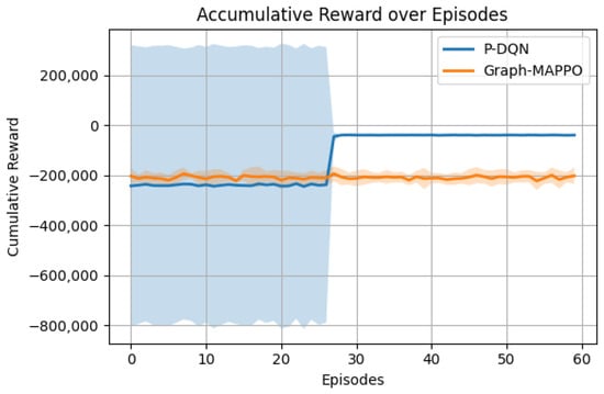
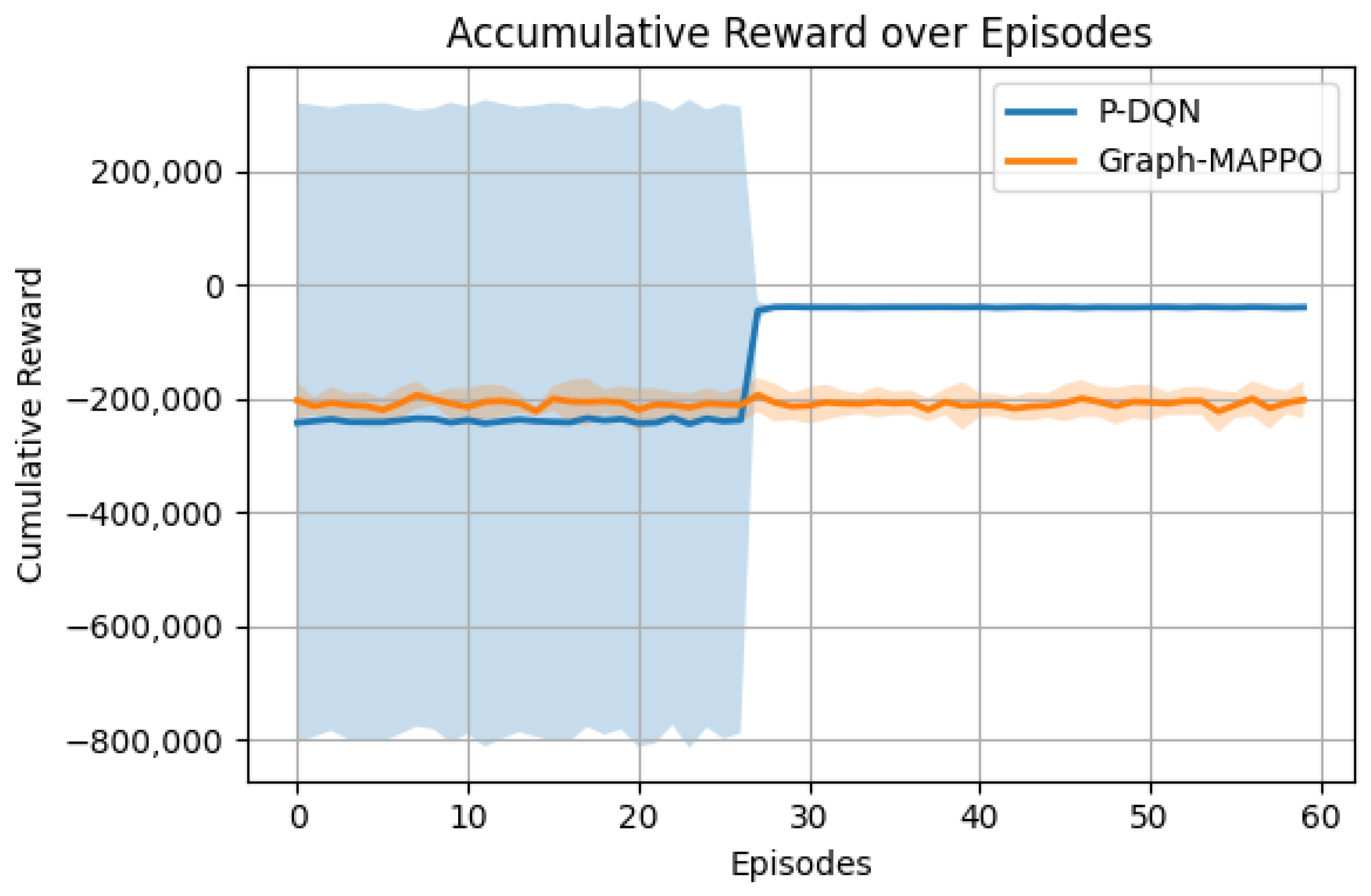
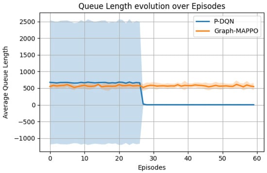
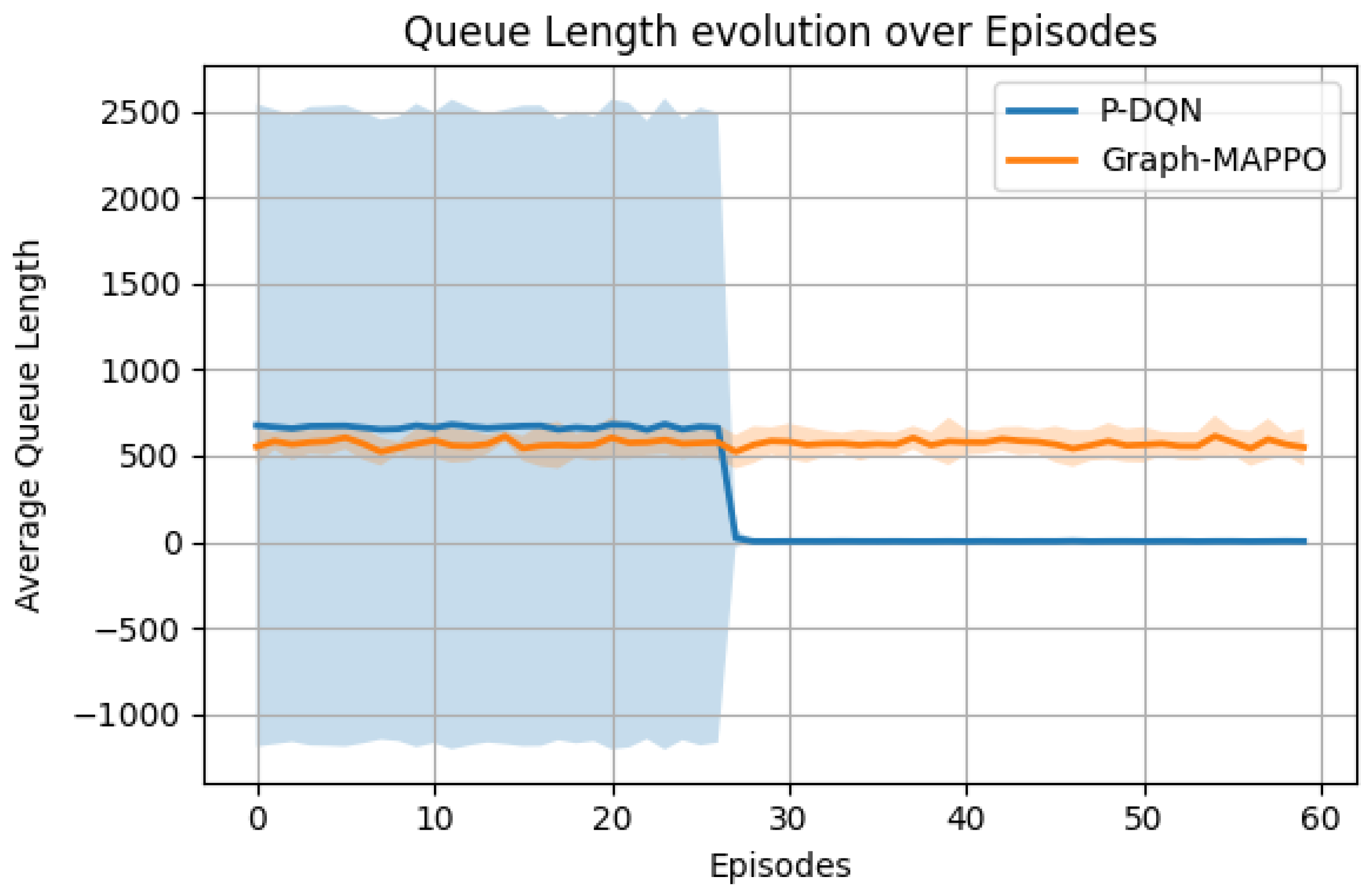
Figure 19, shows both cumulative reward and average queue length plots computed over a number of episodes. It is observed from the cumulative reward curve that P-DQN consistently outperforms Graph-MAPPO. The cumulative reward curve of P-DQN slopes upward after 25 episodes, indicating that the P-DQN agent is effectively learning routing policies that balance traffic flows between the two regions, while Graph-MAPPO’s reward curve remains relatively flat, reflecting slower learning and less efficient policy convergence. Additionally, Figure 20, shows the average traffic queue length computed over a number of episodes. It is observed P-DQN after approximately 25 episodes, the P-DQN agent achieved near-zero average queue length compared to Graph-MAPPO, indicating full queue clearance under the given traffic demand. This behavior arises because the learned continuous control policy effectively balances regional densities while maintaining discharge rates above queue accumulation levels. Given the moderate arrival rates and sufficient service capacity in the simulated environment, the system converges to a stable low-congestion equilibrium. Under higher demand conditions, residual queues would be expected to persist. This performance advantage can be attributed to P-DQN’s parameterized continuous actions, which allow fine-grained traffic control and faster exploration of effective policies, whereas Graph-MAPPO is more sensitive to hyperparameters and may converge slowly in smaller, two-region scenarios.

Figure 19. Comparison of accumulative reward for P-DQN and Graph MAPPO algorithms.

Figure 20. Comparison of average queue length for P-DQN and Graph MAPPO algorithms.

The shaded area around each curve represents the 95% confidence interval across five random seeds, indicating the variability of the agent’s performance for both cumulative reward and queue metrics. Narrow intervals demonstrate consistent learning, while well-separated intervals between P-DQN and Graph-MAPPO highlight statistically significant performance differences. Additionally, Welch’s t-test confirms statistical significance ($p=0.018$, Cohen’s $d=1.4$). These results demonstrate that P-DQN provides faster, more robust learning and superior traffic management compared to a contemporary State-of-the-Art Methods.

5.3. Experimental Results and Findings on Real-World PeMS Traffic Data

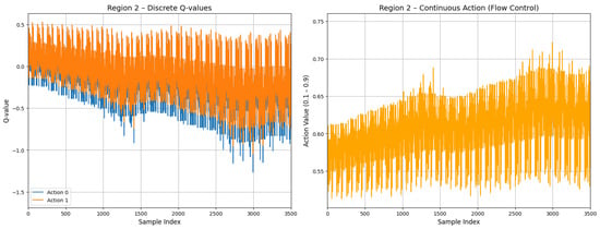
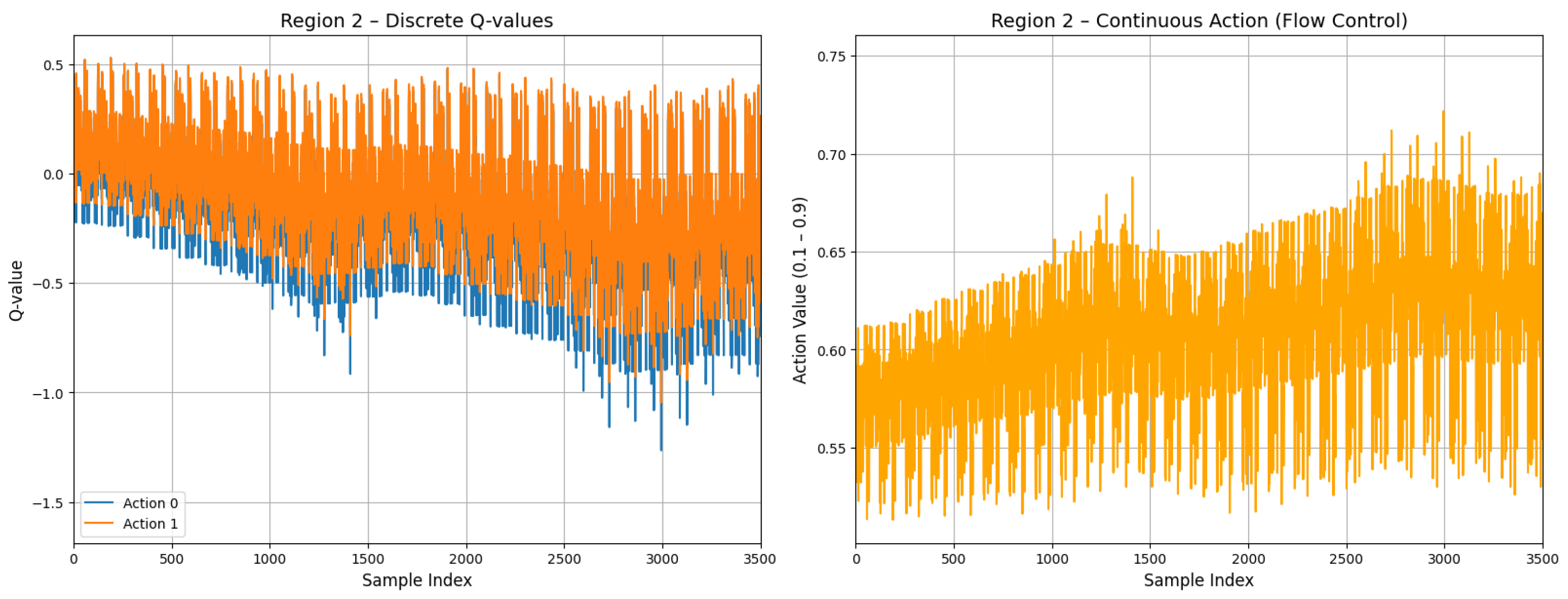
Figure 21 shows the P-DQN agent perimeter control decision outputs for the region region 2. (For completeness, it is noted that Regions 0 and 1 were also analyzed, and their outputs are consistent with the results shown for the regions 2). The plot presents the P-DQN model’s integrated control strategy, combining discrete gating decisions with continuous flow adjustments over time.

Figure 21. P-DQN discrete Q-value and continuous action (flow control).

The left subplot shows the expected positive Q-values for discrete actions, indicating the model’s preferred control under varying traffic conditions, while the right subplot depicts the continuous flow-control action, scaled between 0.1 and 0.9, dynamically modulating traffic flow. Each region’s row allows comparison of discrete and continuous actions across the network, where the discrete action determines whether flow control is applied and the continuous action sets its intensity. The model optimizes a reward function that penalizes high occupancy and imbalance while promoting efficient traffic preservation.

$$\mathcal{R}=-10\mathrm{Var}\left(\mathrm{occupancy}\right)-2\mathrm{Mean}\left(\mathrm{occupancy}\right)+0.5\mathrm{Mean}\left({\mathrm{flow}}_{\mathrm{controlled}}\right)$$

(37)

This formulation encourages the agent to reduce congestion while avoiding excessive flow restriction. This design forces the agent to learn a policy that balances congestion reduction with maintaining throughput.

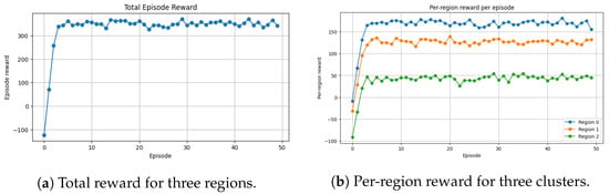
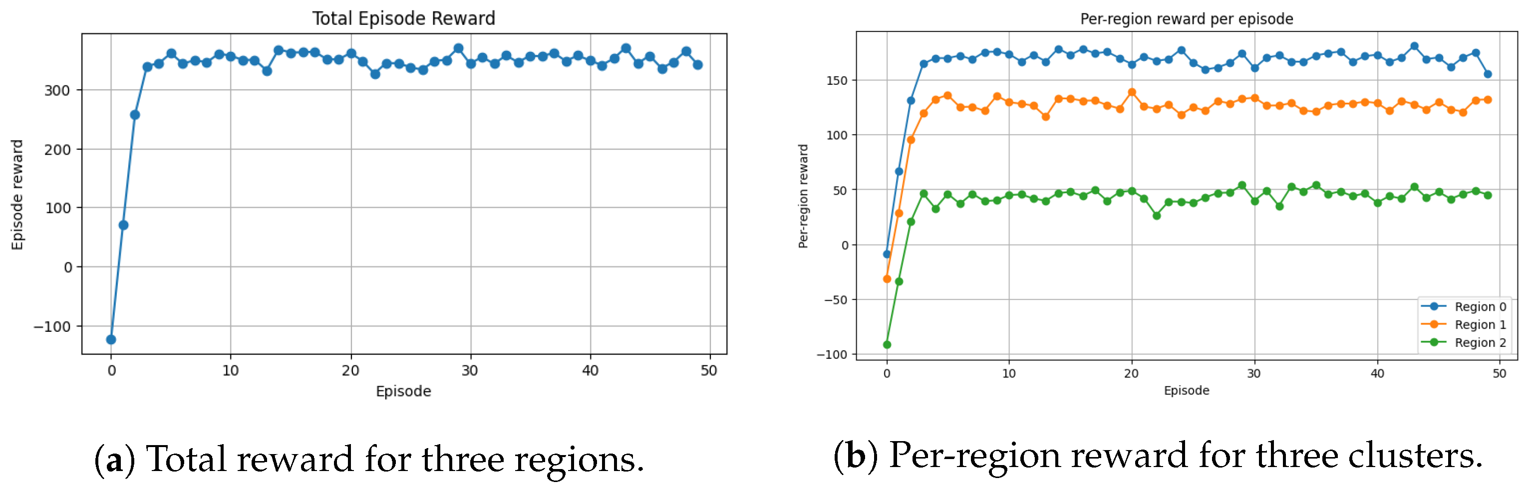
Figure 22a shows episode reward curve to demonstrate the progression of the agent’s learning process. The episode reward increases over first 5 training episodes as the PDQN agent learns to reduce occupancy imbalance and avoid unnecessary flow restrictions. Early episodes show strong noise due to exploration, while later episodes stabilize as the policy converges. Figure 22b shows the per-region reward, each region’s contribution to the total episode reward, based on its occupancy level and controlled flow. Congested regions contribute negatively, while free-flow regions contribute positively. Oscillations remain present throughout training due to the non-stationary nature of real traffic data, exploration noise, and the short 50-step episode horizon. Nevertheless, the overall upward trend indicates that the P-DQN agent successfully learns to minimize occupancy imbalance while preserving acceptable levels of flow.

Figure 22. P-DQN total region reward and per-region reward per episode for the flow rate continuous control.

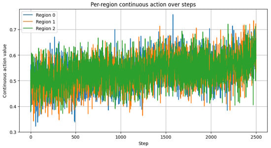
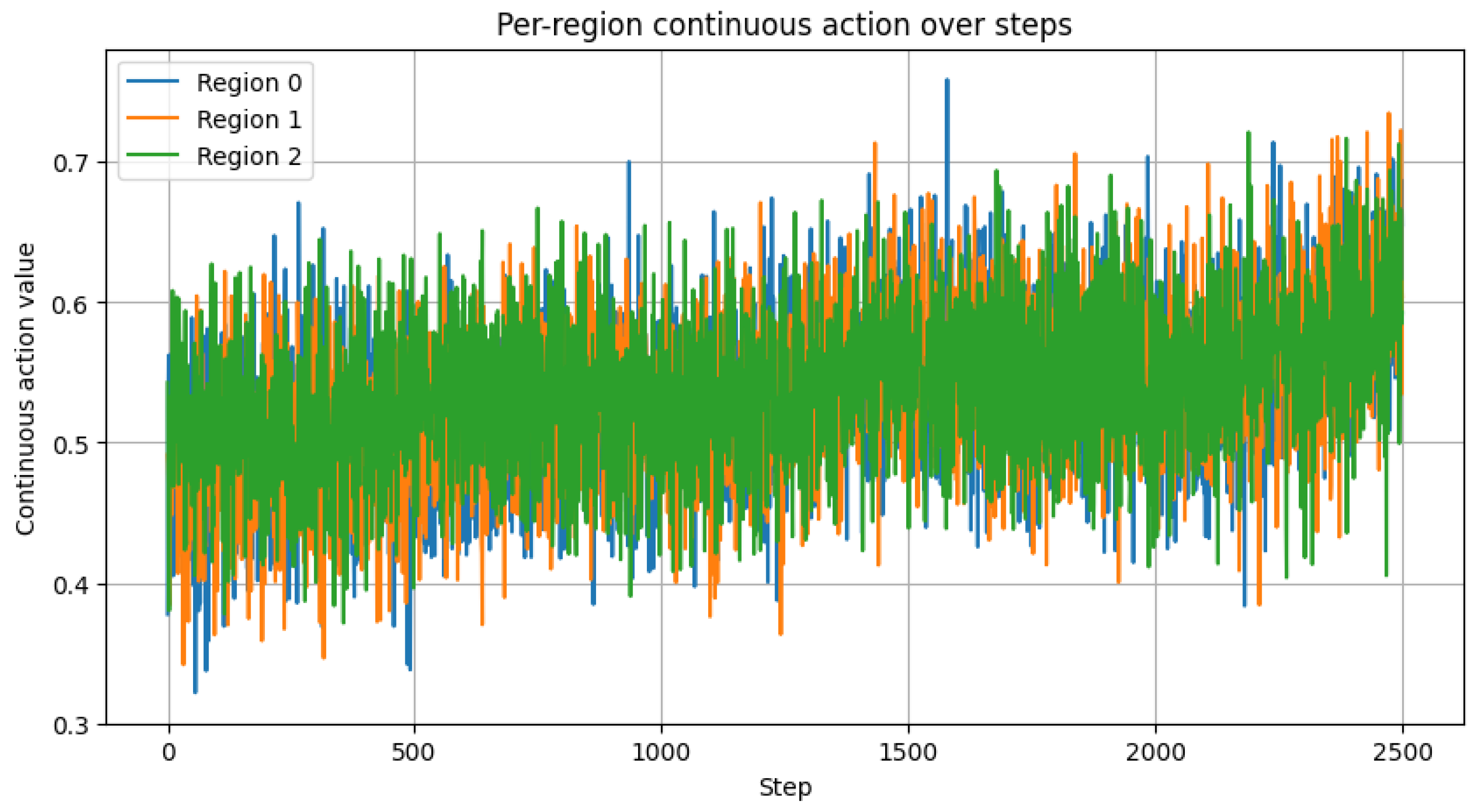
Figure 23 shows the evolution of per-region continuous actions during training. Initially, the actions are highly variable due to exploration and an untrained critic, resulting in unstable reward values. As training progresses, the actions converge toward a moderate range (approximately 0.4–0.7), indicating that the agent has learned a balanced flow-regulation strategy. This convergence reflects the trade-off imposed by the reward function: stronger restriction reduces congestion and occupancy variance, while excessive restriction penalizes throughput. The similarity of the action trajectories across regions demonstrates coordinated control aimed at minimizing inter-regional imbalance, which directly corresponds to the stabilization and improvement observed on the episode reward curve.

Figure 23. P-DQN-predicted actions per region.

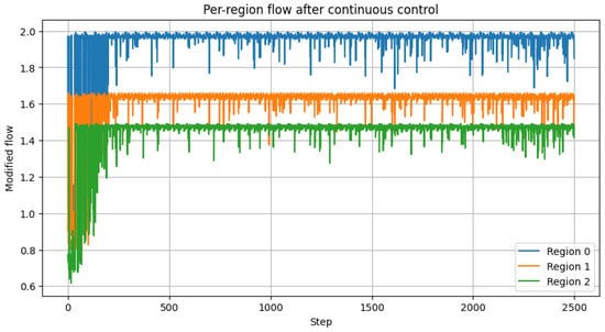
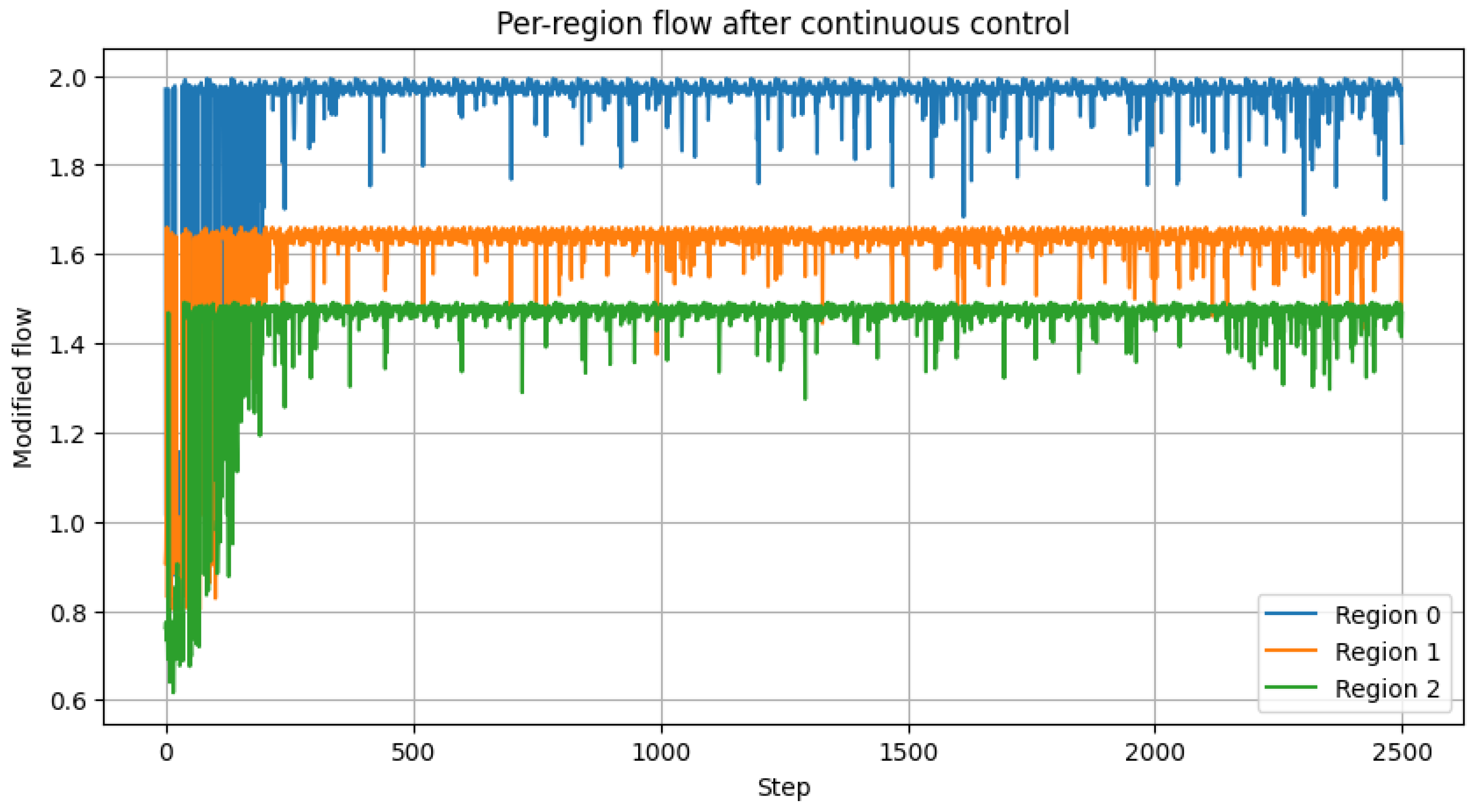
Figure 24 demonstrates the continuous action trajectories providing insight into the agent’s control strategy. The continuous control actions generated by the actor network provide insight into the learned control strategy. Early actions are highly variable due to exploration noise. Over time, the actions stabilize and differentiate across regions. Regions experiencing higher congestion receive larger continuous values, resulting in stronger flow restrictions, while less congested regions receive lower values and remain unobstructed. The plot illustrates the actual traffic flow in each region after control is applied, capturing the combined effect of the discrete control decision (whether control is activated) and the continuous control parameter (control intensity).

Figure 24. P-DQN-predicted traffic flow rate per region.

Variations across regions indicate adaptive flow redistribution, where the PDQN controller selectively restricts flow in more congested regions while maintaining higher flow elsewhere. The absence of sharp oscillations suggests that the learned policy applies smooth and stable control actions, avoiding overly aggressive interventions. Periodic flow reductions correspond to instances when control is activated and scaled by the continuous action. Overall, the plot provides physical interpretability of the learned policy by directly linking PDQN’s hybrid actions to observable traffic-level outcomes and demonstrating how the controller dynamically balances throughput and congestion mitigation in real time. The per-region continuous action values gradually evolve from noisy, exploratory behavior to stable region-specific control patterns. Higher action values indicate stronger flow restriction applied to more congested regions. The controlled flows, show how the learned actions affect actual traffic flows and is defined as

$${\mathrm{flow}}_r^{\mathrm{controlled}}={\mathrm{flow}}_r^{\mathrm{base}}\left(1-a_{c,r}\right)$$

(38)

where $r\in [0,1,2]$ is the region index and $c\in [0,1]$ is the the continuous part of the P-DQN action component. Initially, the flows exhibit instability, but as the policy converges, flow reductions become targeted and consistent with the congestion states of the respective regions. Congested regions experience reduced inflow, whereas free-flowing regions maintain higher throughput.

This, selective behavior validates the agent’s ability to balance congestion mitigation with throughput preservation. The modified flow reflects the effect of the continuous gating action. Over time, flow becomes selectively reduced in congested regions while remaining high in free-flow regions, indicating that the PDQN agent learns appropriate traffic metering. Taken together, the reward curve, continuous actions, and resulting flows indicate that the P-DQN agent successfully learns a stable, interpretable, and region-specific traffic control policy. The agent effectively identifies congested regions and applies appropriate gating actions to minimize congestion propagation while maintaining overall network flow.

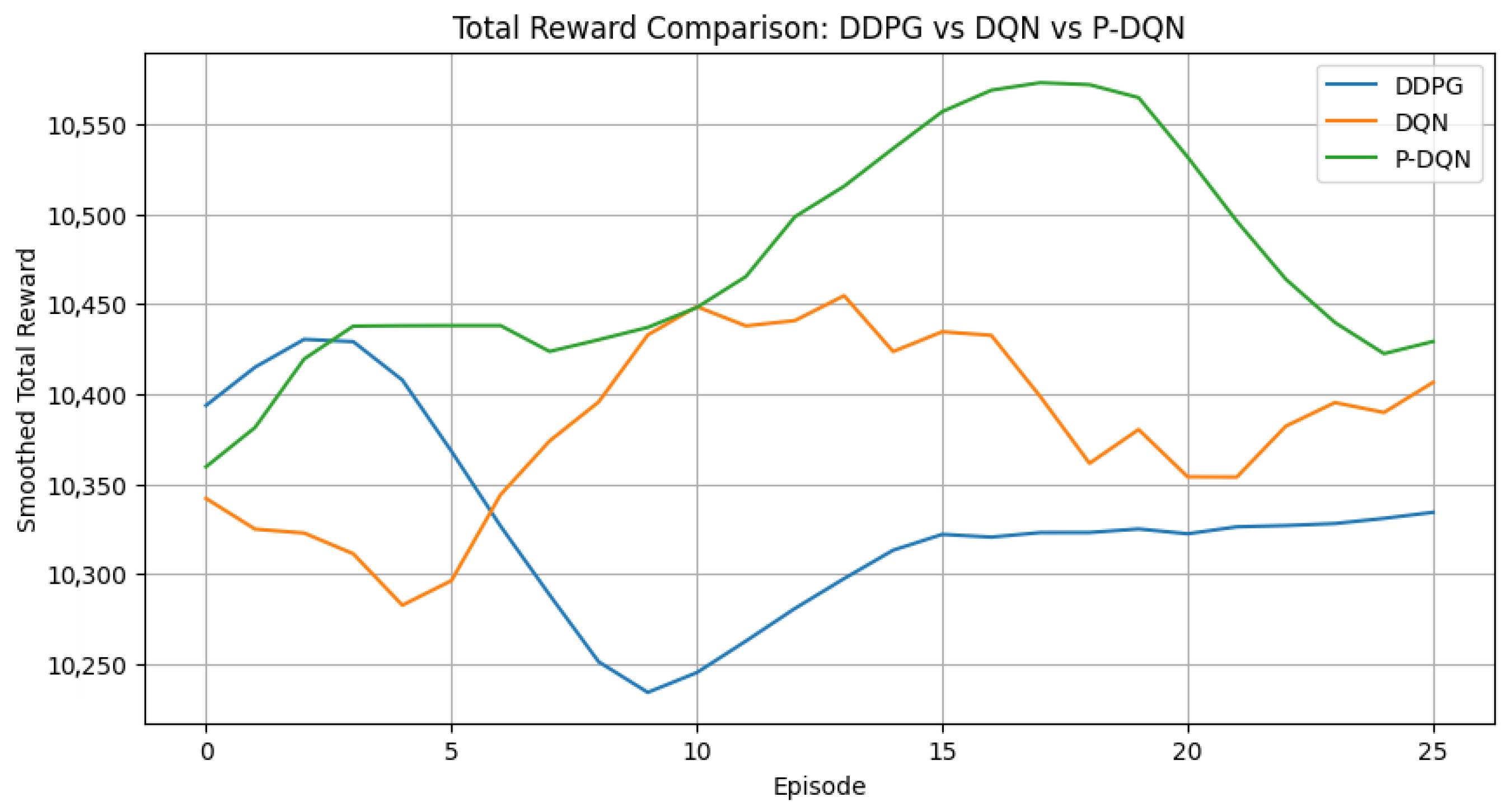
Figure 25 displays per-region reward performance across reinforcement learning models; P-DQN, DDPG and deep Q-network (DQN). The P-DQN achieved the highest average rewards in all regions, with 33.49% against 33.3% for DDPG and 33.2% for DQN, demonstrating stable and consistent improvement over episodes. DDPG shows smooth learning with slightly lower rewards, while DQN exhibits more fluctuations and lower per-region performance. Rewards are designed to maximize traffic flow while penalties account for congestion; overall, P-DQN outperforms the other models in both reward magnitude and consistency across regions.

Figure 25. Total region reward performance comparison for P-DQN, DDPG and DQN algorithms.

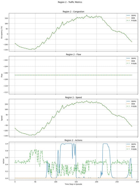
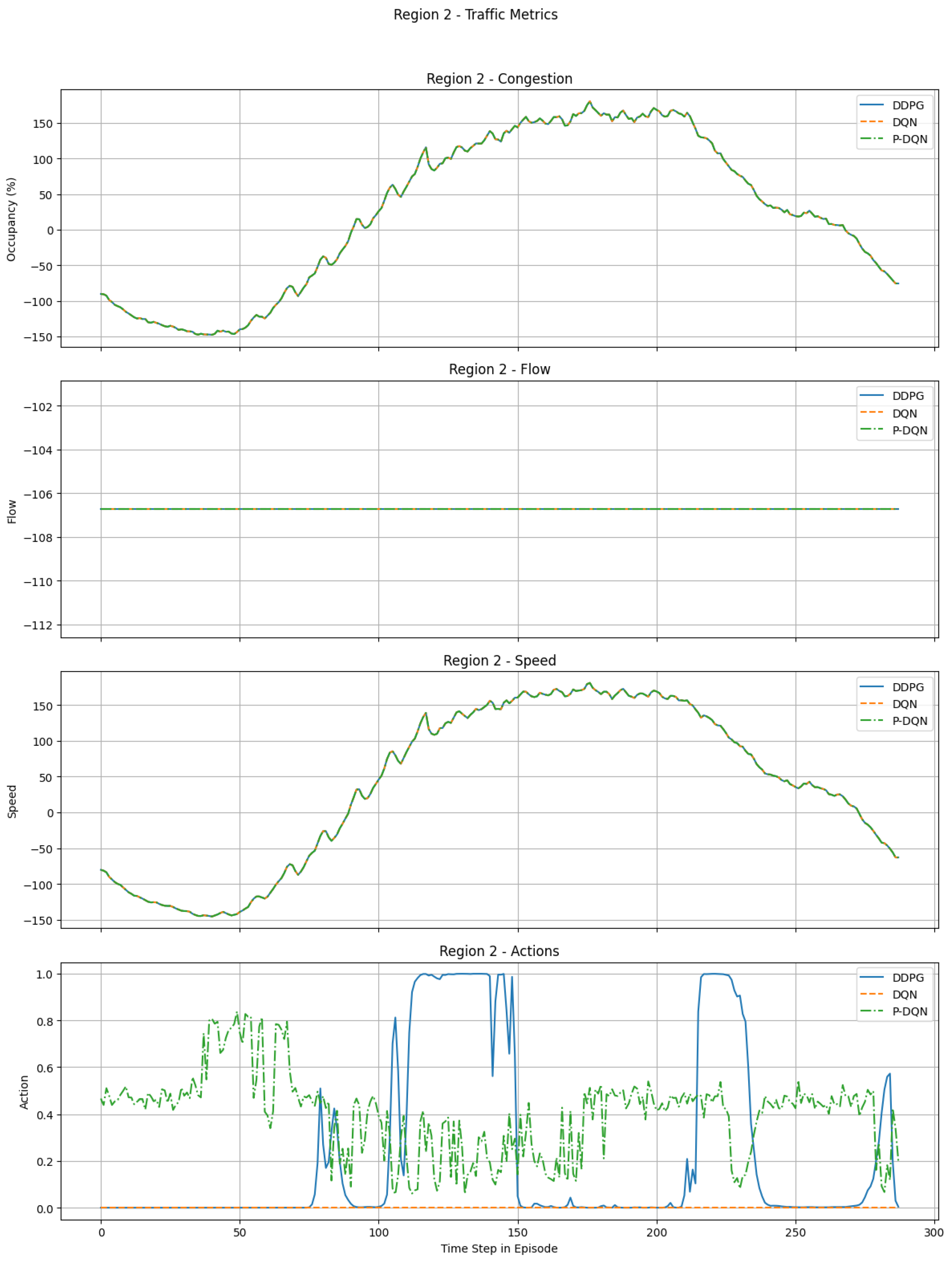
Figure 26 illustrates subplots for the traffic environment states in terms congestion status, flow rate and speed for the region 2. Unlike DQN and DDPG, the P-DQN algorithm delivers smooth, stable, and adaptive control throughout with increasing the episodes. The actions plot shows that DDPG is highly unstable, with large oscillations (instability) and abrupt fluctuations that indicate over-correction and poor control efficiency. The DQN algorithm outputs an almost constant action due to its discrete action space, making it too rigid to respond to changing congestion conditions. In contrast, P-DQN readjusts its actions continuously and moderately, without extreme values or noise, maintaining consistent and stable behavior that intelligently tracks congestion trends. Even though all three algorithms produce the same congestion, flow, and speed plots, P-DQN achieves these outcomes with far more efficient and precise action decisions, demonstrating superior overall control performance.

Figure 26. Comparison of traffic metrics and control actions for P-DQN, DDPG and DQN schemes.

6. Conclusions and Future Work

This study introduced a model-free P-DQNPC framework for multi-region perimeter control, integrating discrete routing and continuous flow-regulation actions. Unlike prior work focused on single-region or purely discrete/continuous controls, P-DQNPC simultaneously optimizes both action types, enabling fine-grained and flexible traffic management. Evaluations on synthetic MFD scenarios and real-world PeMS data show that P-DQNPC consistently outperforms Graph-MAPPO, DQN, DDPG, and No-Control baselines, achieving higher throughput, lower vehicle accumulation, and more stable performance across all regions. Compared to DQN, it overcomes the limitations of purely discrete actions, and compared to DDPG, it delivers greater stability and interpretability. The $95\%$ confidence intervals confirm robustness under stochastic traffic conditions; while the method requires careful hyperparameter tuning and higher computational resources, it is generalizable to other urban networks without region-specific adjustments. Overall, P-DQNPC provides an original, reliable, and practical approach for multi-region traffic control. This work is limited to multi-region perimeter boundary control using macroscopic traffic variables under deterministic demand conditions, with evaluation conducted using real-time PeMS traffic data. Intersection traffic signal control, stochastic demand variations are not considered. Extending the P-DQN framework to these settings is left for future research. Future work will target traffic light control at road intersections with scalable deployment, high-resolution data integration, and enhanced real-time interpretability.

References

- Hu, Z.; Ma, W. Guided deep reinforcement learning for coordinated ramp metering and perimeter control in large scale networks. Transp. Res. Part C Emerg. Technol. 2024, 159, 104461. [Google Scholar] [CrossRef] [Scilit]
- Su, Z.; Chow, A.H.; Fang, C.; Liang, E.; Zhong, R. Hierarchical control for stochastic network traffic with reinforcement learning. Transp. Res. Part B Methodol. 2023, 167, 196–216. [Google Scholar] [CrossRef] [Scilit]
- Haddad, J.; Zheng, Z. Adaptive perimeter control for multi-region accumulation-based models with state delays. Transp. Res. Part B Methodol. 2020, 137, 133–153. [Google Scholar] [CrossRef] [Scilit]
- Xu, Y.; Li, D.; Xi, Y. Perimeter traffic flow control for a multi-region large-scale traffic network with Markov decision process. IEEE Trans. Intell. Transp. Syst. 2024, 25, 4809–4821. [Google Scholar] [CrossRef] [Scilit]
- Su, Z.C.; Chow, A.H.F.; Zheng, N.; Huang, Y.P.; Liang, E.M.; Zhong, R.X. Neuro–dynamic programming for optimal control of macroscopic fundamental diagram systems. Transp. Res. Part C Emerg. Technol. 2020, 116, 102628. [Google Scholar] [CrossRef] [Scilit]
- Guo, Y.; Yang, L.; Hao, S.; Gu, X. Perimeter traffic control for single urban congested region with macroscopic fundamental diagram and boundary conditions. Physica A 2021, 562, 125401. [Google Scholar] [CrossRef] [Scilit]
- Jin, L.; Xu, X.; Wang, Y.; Lazar, A.; Sadabadi, K.F.; Spurlock, C.A.; Needell, Z.; Don, D.R.; Amirgholy, M.; Asudegi, M. Macroscopic traffic modeling using probe vehicle data: A machine learning approach. Data Sci. Transp. 2024, 6, 17. [Google Scholar] [CrossRef] [Scilit]
- Xue, J.; Ka, E.; Feng, Y.; Ukkusuri, S.V. Network macroscopic fundamental diagram-informed graph learning for traffic state imputation. Transp. Res. Part B Methodol. 2024, 189, 102996. [Google Scholar] [CrossRef] [Scilit]
- Ma, W.; Huang, Y.; Zheng, N.; Pan, T.; Zhong, R. Calibration and Uncertainty Quantification of Macroscopic Fundamental Diagrams. arXiv 2025, arXiv:2508.19526. [Google Scholar] [CrossRef] [Scilit]
- Chen, O.; Zhan, Z.; Lv, F. A Comparative Study of Traffic Signal Control Based on Reinforcement Learning Algorithms. World Electr. Veh. J. 2024, 15, 246. [Google Scholar] [CrossRef] [Scilit]
- Lei, T.; Hou, Z.; Ren, Y. Data-driven model free adaptive perimeter control for multi-region urban traffic networks with route choice. IEEE Trans. Intell. Transp. Syst. 2019, 21, 2894–2905. [Google Scholar] [CrossRef] [Scilit]
- Jafari, S.; Shahbazi, Z.; Byun, Y.C. Designing the controller-based urban traffic evaluation and prediction using model predictive approach. Appl. Sci. 2022, 12, 1992. [Google Scholar] [CrossRef] [Scilit]
- Yu, J.; Laharotte, P.A.; Han, Y.; Ma, W.; Leclercq, L. Perimeter control with heterogeneous metering rates for cordon signals: A physics-regularized multi-agent reinforcement learning approach. arXiv 2023, arXiv:2308.12985. [Google Scholar] [CrossRef] [Scilit]
- Jiang, S.; Tran, C.Q.; Keyvan-Ekbatani, M. Regional route guidance with realistic compliance patterns: Application of deep reinforcement learning and MPC. Transp. Res. Part C Emerg. Technol. 2024, 158, 104440. [Google Scholar] [CrossRef] [Scilit]
- Tesone, A.; Pariota, L. Model predictive control based on urban macroscopic fundamental diagram: A city-scale routing application. Transp. Res. Interdiscip. Perspect. 2025, 36, 101816. [Google Scholar] [CrossRef] [Scilit]
- Sirmatel, I.I.; Geroliminis, N. Stabilization of city-scale road traffic networks via macroscopic fundamental diagram-based model predictive perimeter control. Control Eng. Pract. 2021, 109, 104750. [Google Scholar] [CrossRef] [Scilit]
- Yu, H.; Hou, Z. Two-level hierarchical optimal control for urban traffic networks. Transp. A Transp. Sci. 2022, 18, 144–165. [Google Scholar] [CrossRef] [Scilit]
- Michailidis, P.; Michailidis, I.; Lazaridis, C.R.; Kosmatopoulos, E. Traffic signal control via reinforcement learning: A review on applications and innovations. Infrastructures 2025, 10, 114. [Google Scholar] [CrossRef] [Scilit]
- Zhang, C.; Cen, C.; Huang, J. An Overview of Model-Free Adaptive Control for the Wheeled Mobile Robot. World Electr. Veh. J. 2024, 15, 396. [Google Scholar] [CrossRef] [Scilit]
- Wu, J.; Huyan, M. Model-Free Adaptive Control Based on Pattern Class Variables for a Class of Unknown Non-Affine Nonlinear Discrete-Time Systems. Mathematics 2025, 13, 2717. [Google Scholar] [CrossRef] [Scilit]
- Tumu, R.; Shaw Cortez, W.; Drgoňa, J.; Vrabie, D.L.; Glavaski, S. Differentiable Predictive Control for Large-Scale Urban Road Networks. arXiv 2024, arXiv:2406.10433. [Google Scholar] [CrossRef] [Scilit]
- Jiang, S.; Keyvan-Ekbatani, M. Hybrid perimeter control with real-time partitions in heterogeneous urban networks: An integration of deep learning and MPC. Transp. Res. Part C Emerg. Technol. 2023, 154, 104240. [Google Scholar] [CrossRef] [Scilit]
- Ni, W.; Cassidy, M. City-wide traffic control: Modeling impacts of cordon queues. Transp. Res. Part C Emerg. Technol. 2020, 113, 164–175. [Google Scholar] [CrossRef] [Scilit]
- Kampitakis, E.; Vlahogianni, E.I. Decentralized multi-region perimeter control in complex urban environments using reinforcement and imitation learning. Transp. Res. Part C Emerg. Technol. 2025, 178, 105253. [Google Scholar] [CrossRef] [Scilit]
- Zhang, Z.; Zhang, W.; Liu, Y.; Xiong, G. Mean Field Multi-Agent Reinforcement Learning Method for Area Traffic Signal Control. Electronics 2023, 12, 4686. [Google Scholar] [CrossRef] [Scilit]
- Carrillo-González, J.G.; López-Maldonado, G. Method for the Experimental Identification of Variables and Configurations That Modify the Shape of the Macroscopic Fundamental Diagram. Appl. Sci. 2024, 14, 3486. [Google Scholar] [CrossRef] [Scilit]
- Fu, H.; Chen, S.; Chen, K.; Kouvelas, A.; Geroliminis, N. Perimeter control and route guidance of multi-region MFD systems with boundary queues using colored petri nets. IEEE Trans. Intell. Transp. Syst. 2021, 23, 12977–12999. [Google Scholar] [CrossRef] [Scilit]
- Paipuri, M.; Leclercq, L. Bi-modal macroscopic traffic dynamics in a single region. Transp. Res. Part B Methodol. 2020, 133, 257–290. [Google Scholar] [CrossRef] [Scilit]
- Chen, C.; Huang, Y.; Lam, W.H.; Pan, T.; Hsu, S.; Sumalee, A.; Zhong, R. Data efficient reinforcement learning and adaptive optimal perimeter control of network traffic dynamics. Transp. Res. Part C Emerg. Technol. 2022, 142, 103759. [Google Scholar] [CrossRef] [Scilit]
- Zheng, G.; Liu, Y.; Fu, Y.; Zhao, Y.; Zhang, Z. Perimeter control method of road traffic regions based on MFD-DDPG. Sensors 2023, 23, 7975. [Google Scholar] [CrossRef] [Scilit]
- Li, X.; Mercurius, R.C.; Taitler, A.; Wang, X.; Noaeen, M.; Sanner, S.; Abdulhai, B. Perimeter control using deep reinforcement learning: A model-free approach towards homogeneous flow rate optimization. In Proceedings of the 2023 IEEE 26th International Conference on Intelligent Transportation Systems (ITSC), Bilbao, Spain, 24–28 September 2023; pp. 1474–1479. [Google Scholar]
- Zhou, D.; Gayah, V.V. Scalable multi-region perimeter metering control for urban networks: A multi-agent deep reinforcement learning approach. Transp. Res. Part C Emerg. Technol. 2023, 148, 104033. [Google Scholar] [CrossRef] [Scilit]
- Yoon, J.; Kim, S.; Byon, Y.J.; Yeo, H. Design of reinforcement learning for perimeter control using network transmission model based macroscopic traffic simulation. PLoS ONE 2020, 15, e0236655. [Google Scholar] [CrossRef] [Scilit]
- Zhou, D.; Gayah, V.V. Model-free perimeter metering control for two-region urban networks using deep reinforcement learning. Transp. Res. Part C Emerg. Technol. 2021, 124, 102949. [Google Scholar] [CrossRef] [Scilit]
- Yuan, J.; Wu, C.; Teo, K.L.; Xie, J.; Wang, S. Computational method for feedback perimeter control of multiregion urban traffic networks with state-dependent delays. Transp. Res. Part C Emerg. Technol. 2023, 153, 104231. [Google Scholar] [CrossRef] [Scilit]
- Fan, Z.; Su, R.; Zhang, W.; Yu, Y. Hybrid actor-critic reinforcement learning in parameterized action space. arXiv 2019, arXiv:1903.01344. [Google Scholar] [CrossRef] [Scilit]
- Xiong, J.; Wang, Q.; Yang, Z.; Sun, P.; Han, L.; Zheng, Y.; Fu, H.; Zhang, T.; Liu, J.; Liu, H. Parametrized deep q-networks learning: Reinforcement learning with discrete-continuous hybrid action space. arXiv 2018, arXiv:1810.06394. [Google Scholar]
- Horgan, D.; Quan, J.; Budden, D.; Barth-Maron, G.; Hessel, M.; Van Hasselt, H.; Silver, D. Distributed prioritized experience replay. arXiv 2018, arXiv:1803.00933. [Google Scholar] [CrossRef] [Scilit]
- Zhou, D.; Gayah, V.V. Improving deep reinforcement learning-based perimeter metering control methods with domain control knowledge. Transp. Res. Rec. 2023, 2677, 384–405. [Google Scholar] [CrossRef] [Scilit]
- Ren, Y.; Hou, Z.; Sirmatel, I.I.; Geroliminis, N. Data driven model free adaptive iterative learning perimeter control for large-scale urban road networks. Transp. Res. Part C Emerg. Technol. 2020, 115, 102618. [Google Scholar] [CrossRef] [Scilit]
- Li, D.; Hou, Z. Perimeter control of urban traffic networks based on model-free adaptive control. IEEE Trans. Intell. Transp. Syst. 2020, 22, 6460–6472. [Google Scholar] [CrossRef] [Scilit]
- Sun, Y.; Chen, Y. Travel Time Variability in Urban Mobility: Exploring Transportation System Reliability Performance Using Ridesharing Data. Sustainability 2024, 16, 8103. [Google Scholar] [CrossRef] [Scilit]
- California Performance Measurement System. PeMS: Real-Time and Archived Freeway Traffic Data for California Highways. PeMS Collects Real-Time and Archived Freeway Traffic Data, Including Speed, Flow, and Occupancy, from Thousands of Detectors Across California Highways. Available online: https://pems.dot.ca.gov (accessed on 28 October 2025).
Disclaimer/Publisher’s Note: The statements, opinions and data contained in all publications are solely those of the individual author(s) and contributor(s) and not of MDPI and/or the editor(s). MDPI and/or the editor(s) disclaim responsibility for any injury to people or property resulting from any ideas, methods, instructions or products referred to in the content. |
© 2026 by the authors. Licensee MDPI, Basel, Switzerland. This article is an open access article distributed under the terms and conditions of the Creative Commons Attribution (CC BY) license.