


Abstract
This study integrates a Radial Basis Function Neural Network (RBFNN) with Adaptive Dynamic Programming (ADP) to develop an Action-Dependent Heuristic Dynamic Programming (ADHDP) framework for the cost-effective control of an Ice Storage Air-Conditioning (IAC) system. The proposed approach aims to establish a self-learning control strategy for reducing the overall operating cost of the system. In this study, the operational states of the air-conditioning system and the ice-storage/release states of the ice-storage tank are selected as the control variables. To approximate the nonlinear cost-to-go function of the IAC scheduling problem, an RBFNN is employed as the critic-network function approximator. Its local nonlinear approximation capability enables the controller to evaluate the long-term operating costs associated with different ice-storage, ice-melting, and air-conditioning actions. As a result, the proposed ADHDP method can evaluate feasible operating actions and select the action associated with the minimum estimated cost-to-go. Furthermore, an actual IAC system is adopted as the research subject. Field operational data are collected and utilized for system modeling and analysis. Simulations are conducted to compare the Conventional Control Strategy (CCS), ADP, and the ADHDP approach, with operating cost serving as the primary evaluation index. For the investigated representative operating scenario, ADHDP achieved operating costs approximately 7.24% and 1.66% lower than CCS and ADP, respectively. These values represent case-study results under the specific operating conditions considered in this study. Moreover, the ADHDP framework exhibits stronger adaptability to varying cooling loads and electricity pricing conditions, thereby improving the operational efficiency and energy management capability of the IAC system.
1. Introduction
In recent years, with the rapid increase in the use of air-conditioning equipment, the peak electricity demand caused by air-conditioning loads has become one of the major causes of electricity shortages during summer seasons [1,2]. Since the peak usage period of air-conditioning systems usually coincides with periods of high real-time electricity prices, users are required to bear higher electricity costs while simultaneously increasing the peak load pressure on power systems. Therefore, effectively reducing peak electricity demand and improving energy utilization efficiency have become important research topics in the fields of energy management and air-conditioning system control. The Ice-storage Air-Conditioning (IAC) system is considered one of the most effective approaches for addressing this issue [3,4,5]. IAC systems can effectively enhance energy utilization efficiency and resource allocation capability, which is of great significance for energy conservation, carbon reduction, peak load reduction, and environmental protection [6,7]. Consequently, developing a highly efficient and intelligent cost-minimizing control strategy for IAC systems has become an important research direction in the fields of energy management and intelligent control.
In recent years, numerous studies have focused on the scheduling and management strategies of IAC systems, particularly on how different operational strategies affect IAC systems’ profitability. Ref. [8] presents an optimal dispatch model of an ice-storage air-conditioning system for participants to quickly and accurately perform energy saving and transfer energy consumption from the peak load to the partial-peak or off-peak load. Refs. [9,10] employ Model Predictive Control (MPC) to determine the operating schedule by repeatedly solving a finite-horizon optimization problem using predicted cooling loads and system dynamics. Through the rolling optimization mechanism, MPC continuously updates the control action according to the latest system information. MPC’s performance depends on the availability of an accurate prediction model for cooling loads and system dynamics, and a constrained optimization problem must be solved at every control interval. Ref. [11] constructs an optimal scheduling model for the IAC system to participate in the microgrid and analyzes the regulation advantages of the IAC’s cold storage and cold release process and its participation in the scheduling process. Artificial Neural Network is used to construct the function of the cost and operation for each chiller and ice-storage tank and is used to simulate the polynomial function of the cooling load and the cost of power consumption [12,13]. Ref. [14] proposed an optimization strategy for an IAC system considering COP variations and multi-mode switching. This model incorporates four operating modes, which effectively avoids physically inconsistent operations caused by mixed operating modes. Ref. [15] applied a genetic algorithm to determine the charging and discharging schedule of an ice-storage air-conditioning system. Ref. [16] employed particle swarm optimization to improve the operating schedule under time-of-use electricity pricing. Ref. [17] proposed an MPC framework that optimized the operating schedule using predicted cooling-load information. This approach effectively handled time-varying operating conditions but relied on an accurate prediction model. Ref. [18] introduced an adaptive dynamic programming method for nonlinear optimal control of the IAC system. Although the value function was approximated using neural networks, the operating strategy did not explicitly consider the proposed RBFNN-based critic architecture developed in this study. These studies demonstrate that intelligent optimization techniques can effectively reduce operating costs. However, existing methods either require repeated online optimization, depend on accurate prediction models, or provide limited discussion regarding the approximation of the long-term cost function. Most existing approaches rely on predefined operating schedules, simplified mathematical models, or optimization algorithms that require substantial computational effort. Furthermore, the ability to adapt control policies dynamically under varying load demands and electricity pricing conditions remains limited. Therefore, a self-learning and adaptive control framework capable of continuously improving operational decisions is highly desirable.
In the control of IAC systems, Dynamic Programming (DP) can be utilized to determine the optimal operational strategy in order to reduce energy consumption, improve system performance, and satisfy specific performance requirements [19]. However, when dealing with high-dimensional and complex systems, conventional DP often suffers from the “curse of dimensionality,” resulting in a dramatic increase in computational complexity and consequently limiting its practical applications. To address this issue, a composite control method based on Adaptive Dynamic Programming (ADP) has been proposed to solve the profile tracking problem of the hypersonic gliding vehicle (HGV) with multiple constraints [20]. Ref. [21] presented a constrained ADP algorithm to solve general nonlinear nonaffine optimal control problems with known dynamics. Ref. [22] proposed an ADP-based approach to solve the optimal control scheme for energy storage systems with solar renewable energy. ADP combines the concepts of Reinforcement Learning (RL) and DP, enabling effective decision-making and control even when system models or environmental information are incomplete. The control strategy can be continuously adjusted according to real-time system feedback, allowing the system to gradually converge toward the optimal decision outcome.
Recent studies have further extended actor–critic reinforcement learning to nonlinear optimal control problems involving model uncertainty and external disturbances. In this framework, the extended state observer estimates lumped system uncertainties and environmental disturbances, the critic network approximates the value function, and the actor network generates the optimized control input [23]. A neural network was used to approximate unknown nonlinear dynamics, a barrier Lyapunov function was employed to maintain the output errors within prescribed bounds, and an auxiliary system compensated for actuator saturation [24]. Although this approach is not based on reinforcement learning, it demonstrates the importance of incorporating actuator limits and state or output constraints explicitly into neural-network-based control systems. Nevertheless, the performance of an ADP controller depends strongly on the accuracy and efficiency of the selected value-function approximator. For the nonlinear operating characteristics of an IAC system, an appropriate approximator is required to estimate the long-term cost associated with different storage and release decisions. Therefore, this study integrates a Radial Basis Function Neural Network (RBFNN) [25,26] with ADP to develop an action-dependent heuristic dynamic programming framework for cost-oriented control of IAC systems.
Conventional ADHDP architectures generally consist of an actor network and a critic network, where the actor network generates control actions and the critic network evaluates the corresponding long-term cost-to-go. However, the implementation adopted in this study differs from the conventional actor–critic architecture. Because the present IAC scheduling problem contains only three feasible discrete operating modes, all admissible actions can be explicitly enumerated and evaluated by the critic network. Therefore, no separately trained actor network is employed in the proposed implementation. Instead, the RBFNN-based critic estimates the cost-to-go associated with each feasible action, and the action with the minimum estimated cost-to-go is selected as the control decision. Through the self-learning capability of the RBFNN, the control strategy can be continuously adjusted based on real-time operational data, allowing the learned control strategy to be progressively improved based on the estimated long-term operating cost. This study adopts the minimization of the total system operating cost as the primary objective function. The operational states of the air-conditioning system and the ice-storage/release conditions of the ice-storage tank are selected as the system state variables, while chiller on/off control, ice-storage mode switching, and load distribution strategies are defined as the control actions. Based on these variables, an intelligent control model is established using the ADHDP framework. An actual IAC system is employed as the research subject in this study. The case-study results show that the proposed ADHDP-based control method achieved lower operating costs than the Conventional Control Strategy (CCS) and standard ADP under the investigated operating conditions. These results demonstrate the potential feasibility of the proposed method for IAC energy management; however, they should not be interpreted as statistically validated evidence of general superiority.
2. The Description of the Problem
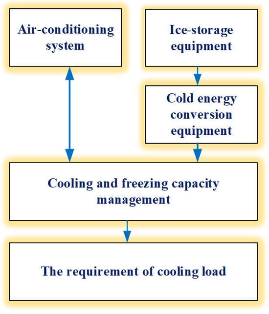
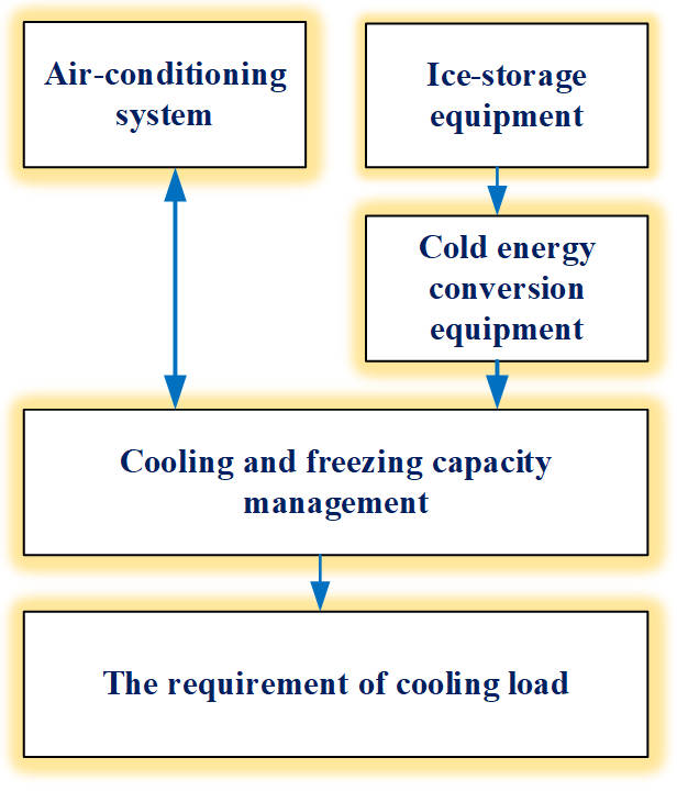
Figure 1 illustrates the configuration of the IAC system, mainly describing the operational relationship among the air-conditioning system, ice-storage equipment, cooling energy conversion devices, and cooling load demand. The entire system is centrally managed by the “Cooling and Freezing Capacity Management” controller, which dynamically adjusts the ice-storage, ice-melting, and air-conditioning operating modes according to the ice-storage condition, cooling load demand, and operational constraints. The primary focus of this study is the optimal control of the cooling storage/release modes to optimize the operational control of the IAC system. The proposed control strategy aims to satisfy cooling load demand while simultaneously minimizing the overall operating cost of the system.
Figure 1.
The configuration of the IAC system.
In this study, to ensure consistency between the physical system and the ADHDP formulation, the discrete-time state model is derived from the cooling-energy balance of the ice-storage tank. The storage state denotes the available cooling energy at the beginning of interval t. The charging and discharging rates, and , are nonnegative thermal-power variables. Therefore, charging increases , whereas discharging and thermal loss decrease it. Assuming piecewise-constant cooling rates over a control interval of duration , integration of the continuous-time energy-balance equation yields
The building cooling-load balance is given by
while the total cooling production of the chiller is
These equations ensure that all cooling-energy flows use consistent signs and thermal-power units. Multiplication by converts thermal power into thermal energy in the storage-state equation. The cooling load of the IAC system is modeled as an hourly varying load, which can be expressed as Equation (4).
Stored cooling energy of the ice-storage tank at time period t.
Stored cooling energy of the ice-storage tank at time period t + 1.
Ice-storage charging/discharging thermal power at time period t.
qI(t) < 0 indicates cold energy storage (ice-storage).
qI(t) > 0 indicates cold energy release (ice-melting).
qI(t) = 0 indicates that the ice-storage equipment is idle.
Conversion efficiency at time period t.
When the entire IAC system requires the air-conditioning chiller to share the cooling load with the ice-storage equipment, the relationship can be expressed by Equation (7).
Cooling load at time period t.
Cooling output of the chiller at time period t.
In this study, the operation problem of the IAC system can be formulated as the minimization of the performance index function, as expressed in Equation (9).
Performance index function at time period t (NT$).
Energy efficiency ratio.
Time-of-Use (TOU) electricity cost at time period t (NT$/kWh) [27].
3. Solution Algorithm
In this study, ADHDP is applied to the control of the IAC system to establish an intelligent self-learning control strategy, thereby reducing the overall operating cost of the system and improving energy utilization efficiency.
3.1. ADP
To establish the ADP model for the IAC system, the system is first transformed into a discrete-time nonlinear state-space representation. The system state variables are defined as Among these variables, is the dynamic state variable, whose evolution is governed by the ice-storage energy-balance equation. In contrast, is not an independent dynamic state. Instead, it is an algebraic operating variable determined from the cooling-load balance and the selected operating mode at each decision interval. It is included as an input to the critic network because it directly characterizes the current operating condition of the chiller and significantly affects the estimated operating cost. Therefore, the RBFNN input vector consists of one dynamic state variable and one algebraic operating variable.
According to Equations (4) and (7), the discrete-time nonlinear state equation of the IAC system can be expressed as follows:
In this study, the cooling load is treated as a known exogenous input to the ADP formulation. The hourly cooling-load profile is obtained from measured operating data of the investigated IAC system and is assumed to be available at each decision interval t. Therefore, no cooling-load forecasting model is employed in the present study. The measured cooling-load value is used in the cooling-load balance to determine the corresponding chiller cooling output and is further incorporated into the state-transition calculation and operating-cost evaluation for each candidate action.
Since the control input is defined as , and , Equation (13) can be further rearranged into a generalized state transition function form as follows.
represents the nonlinear state transition function of the system. To evaluate the control performance of the system under long-term operation, the performance index function is defined as follows:
denotes the system performance index function, represents the discrete-time index, and is the utility function of the system, which is defined as follows:
where α is the power-conversion coefficient, denotes the time-of-use electricity price at time interval t, and γ is the discount factor satisfying 0 ≤ γ ≤ 1. The discount factor determines the relative contribution of future operating costs to the current cost-to-go estimate.
It should be noted that denotes the physical charging/discharging thermal power, whereas denotes the discrete operating-mode command. According to the adopted convention, < 0 represents charging and > 0 represents discharging, while = 1, = 0, and = −1 represent ice storage, direct air-conditioning/idle storage operation, and ice melting, respectively.
From Equation (16), it can be observed that the performance index function at time interval t represents the discounted cumulative value of the utility functions from the current time to an infinite future horizon. Compared with Equation (9), which primarily uses the cooling capacity output as the control evaluation variable, Equation (16) further transforms the system into a dynamic programming framework based on state variables and control inputs. In addition, according to Equation (7), the cooling load during time interval can be regarded as a known constant. Therefore, a fixed relationship exists between and . In other words, once one of these variables is determined, the other variable can also be uniquely specified. Consequently, the system possesses only a single degree of freedom.
Because the action space contains only three discrete operating modes, the selected cost-minimizing action can be obtained by explicit action evaluation rather than by a separate actor network. According to the Bellman Optimality Principle [28], the estimated cost-to-go function can be expressed as follows:
The primary objective of the ADP formulation is to determine a control sequence that minimizes the estimated system performance index. Accordingly, the cost-minimizing control action is obtained by explicitly comparing the estimated cost-to-go values of all feasible discrete actions, as expressed in Equation (18).
returns the control input that minimizes the objective function.
Where denotes the control action that minimizes the estimated objective function over the finite set of feasible operating modes.
3.2. ADHDP
In the present IAC scheduling problem, the long-term operating cost is a nonlinear function of the cooling load, electricity price, ice-storage state, and control action. Therefore, an RBFNN is adopted as the critic-network approximator to estimate the cost-to-go function for the feasible operating modes. To overcome these limitations, this study integrates an RBFNN into the ADP framework and develops an ADHDP-based controller for cost-oriented operation of the IAC system. ADHDP usually employs two neural networks: an actor network that generates the control action and a critic network that estimates the corresponding value function. Since the present IAC system contains only three feasible operating modes, namely ice storage, direct air-conditioning, and ice melting, the action space is finite and can be exhaustively evaluated. Therefore, the proposed controller does not employ a separate actor network. Instead, all admissible operating actions are evaluated individually by the RBFNN critic, and the action associated with the minimum estimated cost-to-go is selected as the cost-minimizing control decision according to the critic estimate. The RBFNN is employed as the function approximator of the critic network to estimate the nonlinear cost-to-go function and improve the learning efficiency of the control system. RBFNN can exhibit faster convergence speed, simpler network architecture, and superior local approximation capability. These advantages enable the proposed controller to effectively learn the nonlinear relationships among cooling load demand, electricity pricing, and ice-storage status, thereby improving the control performance of the IAC system.
The RBFNN employed in this study consists of an input layer, a hidden layer, and an output layer. The hidden neurons utilize Gaussian radial basis functions to perform nonlinear transformation of the input data. The output of the i-th hidden neuron is expressed as:
: output of the -th hidden neuron
: input vector
: center of the -th radial basis function
: width parameter
The estimated cost-to-go function generated by the RBFNN can be expressed as:
: connection weights
: estimated performance index function
: number of hidden neurons
In the proposed ADHDP implementation, the critic network approximates the value function using the physical operating state of the IAC system. Therefore, the RBFNN input is defined as
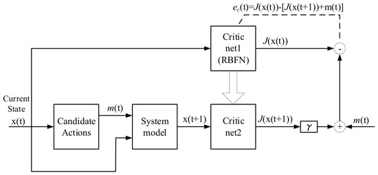
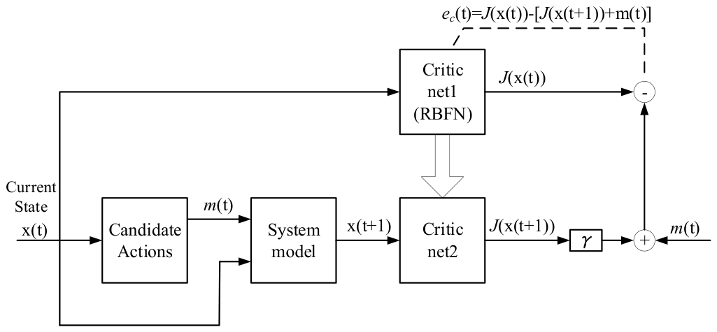
Figure 2 illustrates the critic-based action-evaluation framework adopted in this study. Unlike a conventional actor–critic ADHDP architecture, the proposed implementation does not employ a separately trained actor network. At each decision interval, all three feasible operating actions are explicitly evaluated. For each candidate action, the system model determines the corresponding operating transition, and the RBFNN critic estimates the associated cost-to-go. The action with the minimum estimated cost-to-go is then selected as the control decision. Its primary objective is to progressively obtain the cost-minimizing control strategy for the IAC system through an RBFNN approach.
Figure 2.
The operational framework of ADHDP.
From Figure 2, the current system state is represented by and is fed into the Candidate actions. The function of the Candidate actions is to generate the control input according to the current system state, thereby determining the operational strategy of the IAC system at the current time instant, such as the ice-storage or ice-melting control of ice-storage. This control input is then sent to the System Model to simulate the dynamic behavior of the system under the applied control action, resulting in the next-state . Subsequently, the Critic Network is mainly responsible for evaluating the performance of the current control strategy. As shown in Figure 2, two critic networks are employed: Critic net1 and Critic net2. Critic net1 receives the current state as input and outputs the corresponding performance function . In contrast, Critic net2 receives the next-state and outputs the future performance function . The future performance function is further weighted by the discount factor γ, which represents the importance of future costs or benefits in the current decision-making process. By combining this term with the discounted future performance function, a target value can be constructed and compared with the current output generated by the critic network. The difference between these two quantities forms the error signal of the critic network, denoted as , which can be mathematically expressed as follows:
The training procedure of the critic network in ADHDP is described as follows.
- A.
- Initialize
- ➢
- Construct Critic Net1 and Critic Net2 using identical RBFNN architectures.
- ➢
- Initialize all connection weights randomly.
- ➢
- Set the convergence tolerances and .
- B.
- Training iterationStep 1. Collect the training data for the critic network, including and randomly generate ice-storage, ice-melting, and idle actions to train the neural network.Step 2. Obtain from critic net2, and use as the target output for in critic net1 for training.Step 3. After critic net1 reaches the specified error value , copy net1 to net2 so that net2 and net1 have identical weight values.Step 4. Repeat Steps 2 to 3 until , indicating that . Then proceed to the next step.Step 5. Repeat Steps 2 to 4 until , indicating that holds for . Then proceed to the next step.Step 6. Select critic net1 as the fully trained critic network.
Two critic networks are employed during training. Critic Net1 is updated using the Bellman target, while Critic Net2 serves as the target network for value evaluation. After Critic Net1 has completed one training iteration, all network parameters, including the RBF weights, basis-function centers, and widths, are copied to Critic Net2 before the next iteration. The proposed method is developed within the ADHDP framework; its implementation differs from the conventional actor–critic ADHDP architecture. More precisely, it can be regarded as a critic-based, action-dependent value-iteration implementation of ADHDP, in which policy improvement is performed by explicit minimization over the finite action set rather than by a separately trained actor network. By integrating RBFNN and ADHDP, the proposed controller can effectively approximate the nonlinear cost-to-go function and dynamically select the control action associated with the minimum estimated cost-to-go under varying cooling-load and electricity-price conditions. Under the investigated case-study conditions, this critic-based implementation enables the controller to select actions according to their estimated long-term operating costs and results in lower operating costs than the compared ADP-based strategy.
3.3. Implementing the ADHDP for IAC
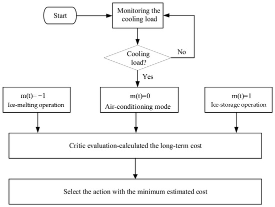
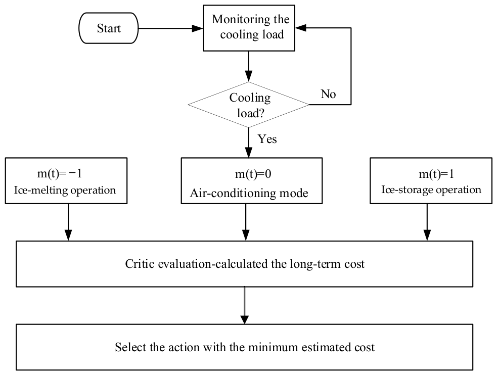
Figure 3 illustrates the proposed ADHDP-based optimal control flowchart for the IAC system. During the control decision-making stage, the control actions in this study are categorized into three possible operating states as follows.
Figure 3.
ADHDP-based control flowchart.
- : Air-conditioning operation mode
- : Ice-storage operation mode
- : Ice-melting operation mode
The procedure of implementing the ADHDP in the IAC system is described as follows.
- A.
- Initialization
Before the system begins operation, the relevant parameters and initial conditions must first be determined. The procedure is described as follows:
- Determine the control time interval D
Set a 24 h daily operation period.
- 2.
- Determine the air-conditioning cooling load
Define the cooling load demand for each time interval according to the building air-conditioning requirements.
- 3.
- Determine the electricity pricing function
Incorporate the TOU electricity pricing information for each time interval into the system.
- 4.
- Randomly generate the initial control action m(t) for each time interval
The initial control strategy is randomly generated by the system and serves as the initial solution for subsequent ADHDP learning and optimization processes.
- B.
- Iterative Learning Process
- Step 1: State Data Collection and Utility Function Calculation
The system first collects the current state data and calculates the immediate utility function:
α is the weighting parameter, denotes the time-varying electricity price, and represents the current system state. This utility function is mainly used to evaluate the operating cost or benefit of the system under the current control strategy.
- Step 2: Critic Network Training
According to the ADHDP algorithm, the Critic Network is trained using the current system state, control input, and utility function so that it can learn the long-term performance value corresponding to different control strategies and gradually approximate the estimated cost-to-go function.
- Step 3: Applying the Critic Network to the Learning Process
After the training process is completed, the Critic Network is embedded into the Learning Optimal Control process. At this stage, the Critic Network can evaluate the effectiveness of different control actions in real time according to the current system state.
- Step 4: Selection of the Cost-Minimizing Control Action
The system compares the outputs of the Critic Network corresponding to different control actions and selects the action with the minimum critic output as the control decision for the current interval. Since the Critic Network output represents the long-term system cost or performance index, a smaller output value indicates better control performance.
- Step 5: Obtaining the Learned Control Sequence
Through repeated iterative learning, the system can ultimately obtain the control sequence:
where denotes the control action at each time interval. Through this control sequence, the IAC system can automatically adjust the ice-storage, ice-melting, and air-conditioning operating modes according to load demand and electricity pricing conditions at different times, thereby reducing energy costs and improving system efficiency.
4. Simulation Results
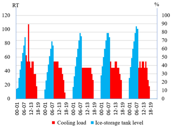
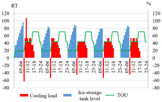
In this simulation study, the administrative building of an electrical equipment company is selected as the experimental target. Two brine chillers are employed to supply the IAC system of the administrative building. This study analyzes the hourly air-conditioning load, TOU electricity pricing, and various operating modes of the system. For the summer season, the period from 15 July to 19 July 2024 was selected as the representative week (five working days) for control-performance analysis. Figure 4 illustrates the operating behavior of the proposed controller under the investigated operating conditions, including the evolution of the ice-storage energy and chiller output.
Figure 4.
The cooling load and the ice-storage tank level during the representative summer week.
Figure 4 illustrates the operational variation between the cooling load and the ice-storage tank level (%) during the summer period. As shown in Figure 4, the cooling load is relatively low during off-peak nighttime hours. Therefore, the system utilizes the lower electricity price period to produce ice, resulting in a gradual increase in the ice-storage tank level. During daytime peak periods, as the cooling load increases, the ice-storage tank level gradually decreases. This indicates that the system begins to release the stored cooling energy to satisfy the cooling load. Overall, the system exhibits a cyclic operating pattern of “ice-storage at night and ice-melting during the daytime.” This operating strategy can effectively reduce peak electricity demand, achieve peak shaving and load leveling, and lower air-conditioning operating costs. The results demonstrate that the IAC system possesses excellent energy management and load regulation capabilities.
4.1. CCS Control of IAC System
Table 1 presents the comparison results of electricity consumption and electricity cost for the CCS control during the representative summer week. The operational cost differences under the two-stage and three-stage electricity pricing schemes are also compared. As shown in Table 1, the electricity consumption during the ice-melting stage is significantly higher than that during the ice-storage stage. Among all weekdays, Monday exhibits the highest electricity consumption for ice storage, reaching 875.9 kWh, while the electricity consumption during ice-melting ranges from 79.4 to 93.4 kWh. This indicates that the system primarily performs large-scale ice storage during off-peak periods and releases the stored cooling energy during peak periods to reduce the air-conditioning load. In terms of electricity cost, the total weekly electricity cost under the two-stage pricing scheme is NT$6711, whereas the total cost under the three-stage pricing scheme is NT$6163. This represents a reduction of approximately NT$548, corresponding to an electricity cost saving of about 8.17% compared with the two-stage pricing scheme. From the daily results, it can also be observed that the electricity cost under the three-stage pricing scheme is consistently lower than that under the two-stage pricing scheme for every day of the week. This demonstrates that the ice-storage air-conditioning system can effectively utilize off-peak and semi-peak periods for energy storage operations, thereby further reducing peak-period electricity costs. Overall, the results indicate that under high summer cooling-load conditions, the conventional ice-storage and ice-melting operation mode combined with the three-stage electricity pricing scheme provides superior economic benefits.
Table 1.
The comparison results of electricity consumption and electricity cost for the CCS control.
Table 2 presents the operating actions of the IAC system during each time interval of the representative summer week. In Table 2, the value “1” represents the ice-storage mode, “−1” represents the ice-melting mode, and “0” indicates that the system stops both ice-storage and ice-melting operations. From Table 2, it can be observed that the control strategies from Monday to Friday are identical, indicating that the system operation exhibits stable and fixed scheduling characteristics.
Table 2.
The operating actions of the IAC system during each time interval of the representative summer week.
4.2. ADP Control of IAC System
Table 3 presents the control strategy using ADP. Table 3 also indicates that both control strategies generally follow the principle of “ice-storage during off-peak periods and ice-melting during peak periods”. However, the ADP-based control strategy demonstrates greater flexibility and adaptability during certain operating periods. Both strategies perform ice storage during off-peak nighttime hours and utilize ice melting to provide cooling during high daytime load periods. After the cooling load decreases in the evening, both systems stop the ice storage and ice-melting operations (control action equals 0). Nevertheless, the most significant difference between the two control strategies occurs during the 08:00–09:00 period. In the CCS, the system switches to the ice-melting mode at 08:00. In contrast, the ADP-based control strategy maintains the ice-storage mode until 09:00 (highlighted in the yellow region). This result indicates that, after learning the variations in electricity pricing and cooling load demand, the ADP controller determines that extending the ice-storage period by one additional hour can achieve better overall operational performance.
Table 3.
The control strategy using ADP.
This finding demonstrates that ADP does not rely on a fixed time-based control strategy; instead, it can dynamically adjust the selected control action according to the system state and cost function. Furthermore, by delaying the start time of ice melting, the ADP control strategy allows the system to store more cooling energy for daytime operation, thereby enhancing the cooling supply capability during peak periods. This reduces the direct operating demand of the chiller system and consequently decreases peak electricity consumption and electricity cost. Compared with CCS, the ADP-based control strategy exhibits superior intelligence and adaptability, enabling adaptive adjustments under different seasonal conditions, load demands, and time-of-use electricity pricing schemes.
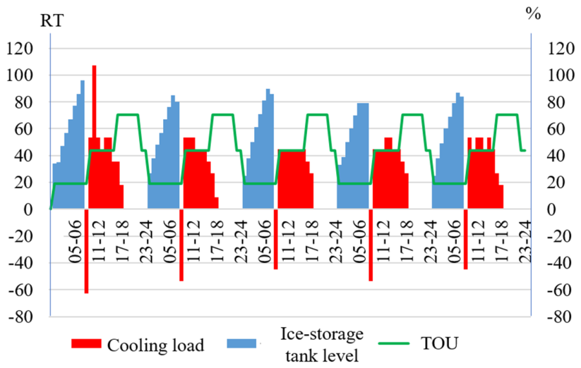
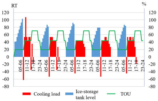
Figure 5 presents the operating characteristics of the IAC system using ADP. Figure 5 mainly presents the relationship among the cooling load, ice-storage percentage, and time-of-use electricity pricing. From the figure, it can be observed that the system operating strategy adjusts the ice-storage and ice-melting operations according to the electricity price in order to reduce operating electricity cost. During the off-peak nighttime period (approximately from 23:00 to 08:00 of the following day), the electricity price is relatively low. Therefore, the system performs ice storage for thermal energy storage, causing the ice-storage level to gradually increase. The blue region in the figure exhibits an upward trend, with the ice-storage percentage reaching nearly 90% or higher. In this stage, low-cost electricity is utilized for cold-energy storage, effectively reducing electricity expenses during subsequent peak periods. When the system enters daytime peak or semi-peak periods, the electricity price increases, and the system begins to perform ice-melting to provide cooling, thereby reducing the power consumption required for direct chiller operation. During this process, the blue ice-storage level gradually decreases, while the red air-conditioning load is partially supplied by the ice-melting system. It can be clearly observed from the figure that the ice-storage level decreases progressively as the daytime cooling load increases, indicating that the system is releasing the previously stored cooling energy.
Figure 5.
The operational characteristics of the IAC system by using ADP.
The ADP-based scheduling strategy for the IAC system can automatically adjust the timing of ice-storage and ice-melting according to variations in cooling load demand and electricity pricing. This enables the energy storage system to store energy during low-price periods and release energy during high-price periods. Consequently, the strategy not only improves energy utilization efficiency but also effectively reduces the operating electricity cost of the air-conditioning system, thereby illustrating the potential economic benefit under the investigated operating conditions.
4.3. ADHDP Control of IAC System
Table 4 presents the cost-minimizing control strategy using ADHDP for the representative summer week. By comparing the results with the aforementioned ADP cost-minimizing control strategy, it can be observed that both approaches maintain the same fundamental control framework. In both tables, the system remains in the ice-storage mode from 00:00 to 09:00 and switches to the ice-melting mode from approximately 09:00 to 18:00, indicating that the overall ADP-based control strategy still follows the core principle of “energy storage during off-peak periods and energy release during peak periods.” However, the ADHDP control strategy demonstrates greater dynamic adjustment capability and flexibility. The control strategy is no longer based on a simple fixed schedule; instead, it can perform more refined optimization adjustments according to real-time load demand, ice-storage status, and variations in time-of-use electricity pricing. When the system determines that re-entering the ice-melting mode during certain periods can provide better overall economic benefits, it temporarily stops ice melting and resumes ice storage to maintain a higher thermal storage capacity and subsequent cooling supply capability. The re-ice-melting strategy observed during certain periods in the ADHDP results also indicates that ADHDP possesses a certain degree of predictive and adaptive capability. Compared with the previous control strategy, which relied more heavily on fixed operational logic, Table 4 demonstrates that ADHDP can more effectively utilize electricity price differences and load variations across different time periods, thereby improving the energy scheduling efficiency of the ice-storage system.
Table 4.
The cost-minimizing control strategy using ADHDP.
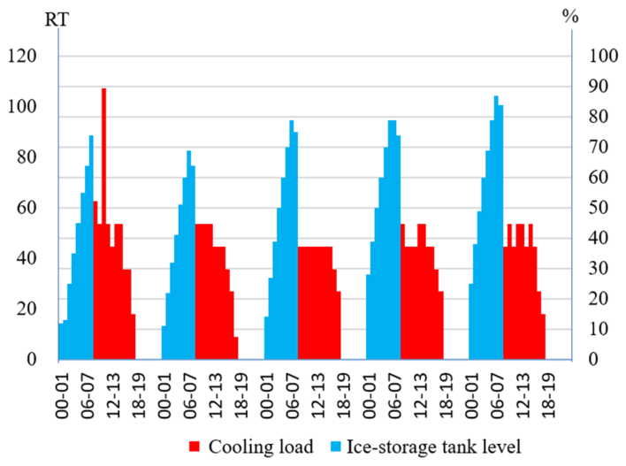
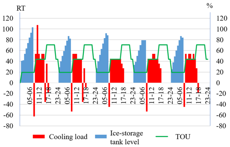
Figure 6 presents the operating characteristics of the ACS system using ADHDP. Compared with the ADP-based scheduling strategy, the ADHDP scheduling exhibits more pronounced dynamic adjustment characteristics, enabling the system to automatically adjust ice-storage and ice-melting operations according to load demand and electricity pricing conditions at different time periods in order to achieve better operational performance. As observed in Figure 6, during the nighttime off-peak period, the system continuously performs ice storage, causing the ice-storage level to gradually increase. The blue ice-storage curve approaches full capacity during the early morning hours. Since the electricity price is relatively low during this period, the ADHDP control strategy preferentially utilizes low-cost electricity for cold-energy storage, thereby reducing electricity costs during the subsequent daytime high-price periods. When the system enters daytime periods characterized by high cooling loads and high electricity prices, it begins to perform ice melting to provide cooling. Consequently, the ice-storage level gradually decreases, indicating that the system is releasing the previously stored cooling energy to satisfy the air-conditioning load demand while reducing the direct operating requirement of the chiller system. From the variations in the red air-conditioning load curve and the blue ice-storage level curve, it can be observed that ADHDP can dynamically adjust the utilization of cooling energy according to load variations, enabling the system to operate more smoothly and efficiently.
Figure 6.
The operating characteristics obtained from the IAC system using ADHDP.
Table 5 presents the comparison results of air-conditioning operating costs for the representative summer week under three different control methods: CCS, ADP, and ADHDP. From Table 5, it can be clearly observed that as the intelligence level of the control strategy increases, the operating cost of the IAC system gradually decreases. This demonstrates that better control strategies can effectively improve both the energy-saving performance and the economic benefits of the ice-storage air-conditioning system. In terms of daily operating cost, the traditional IAC control exhibits the highest cost among the three methods. These results indicate that both ADP and ADHDP can reduce the operating cost of the air-conditioning system through better control strategies, with ADHDP demonstrating superior control performance. From the comparison of total weekly operating cost, the traditional IAC control method results in a total cost of NT$3652.8, while the ADP control strategy reduces the total cost to NT$3445.9, corresponding to an approximate reduction of 5.66%. The ADHDP control strategy further reduces the total cost to NT$3388.5, representing an approximate reduction of 7.24% compared with traditional control. Furthermore, compared with ADP, ADHDP achieves an additional cost reduction of approximately 1.66%.
Table 5.
The comparison of operating costs under three different control methods.
The proposed method is compared with the CCS and the conventional ADP controller. CCS represents the rule-based operating strategy currently adopted in practical IAC systems and therefore serves as the practical engineering baseline. ADP is selected because the proposed method is developed as an enhanced ADP framework using an RBFNN critic. Consequently, comparison with conventional ADP directly demonstrates the contribution of the proposed value-function approximation. Although DP and MPC are widely recognized benchmark approaches for optimal control, they are not included in the present study. DP generally becomes computationally expensive as the discretization of the state and action spaces increases, whereas MPC requires an accurate predictive model of future cooling loads and system dynamics. The implementation and evaluation of these benchmark methods are therefore considered important directions for future work. In addition, the present study evaluates the proposed controller using one representative operating scenario under identical cooling load and electricity-price conditions for all compared methods. The reported operating-cost reductions reflect the performance under the investigated case study rather than statistical averages obtained from repeated experiments. Since the current implementation does not include repeated training with different random initializations or Monte Carlo simulations, statistical measures of variability and significance are not reported. Therefore, the observed cost reductions should be interpreted as case-study outcomes rather than statistically validated performance gains.
5. Conclusions
This study proposed a self-learning ADHDP-based control method for an IAC system and evaluated it using operational data from a representative summer week. Simulation analysis and validation were conducted using operational data collected from a representative summer week. The results demonstrate that the proposed ADHDP control framework can effectively improve the conventional fixed ice-storage and ice-melting control strategy while enhancing the energy management capability and operational performance of the IAC system. In the analysis of better control strategies, ADHDP not only maintains the fundamental principle of “ice-storage during off-peak periods and ice-melting during peak periods,” but also performs detailed adjustments according to electricity pricing and load conditions at different time intervals. During certain periods, the system reactivates the ice-storage mode to maintain a higher thermal storage capacity and subsequent cooling supply capability, indicating that the ADHDP-based strategy exhibited more flexible action adjustments under the investigated cooling-load and electricity-price conditions. For the representative summer-week case study considered in this work, the proposed ADHDP approach resulted in operating costs approximately 7.24% lower than those of the conventional IAC control strategy and 1.66% lower than those of ADP. These results demonstrate the potential of the proposed controller under the investigated operating conditions; however, they should be interpreted as case-study results rather than statistically validated performance gains. The proposed ADHDP-based control method can serve as an important reference for energy management systems in intelligent buildings, smart grids, and large-scale public facilities. Although all control methods are evaluated under identical operating conditions, repeated experiments with different random initializations and operating scenarios would provide a more comprehensive assessment of the robustness of the proposed controller.
The present case study contains two state variables and three discrete operating modes; therefore, the results should not be interpreted as evidence of scalability to high-dimensional systems. The present study does not provide theoretical proof of convergence or global optimality for the proposed RBFNN-based ADHDP framework. The effectiveness of the controller is evaluated through the operating-cost reduction achieved in the case study. Future work will investigate theoretical convergence properties of the proposed critic-learning procedure and will include Bellman residual analysis, critic-weight convergence, multiple random initializations, and statistical performance evaluation to provide stronger evidence regarding learning stability and robustness. It will extend the framework to multiple chillers and ice-storage tanks, continuous cooling-power allocation, weather and indoor-temperature states, equipment start-up constraints, and demand-response signals. Such extensions will also require systematic evaluation of computational complexity, convergence, and scalability.
Author Contributions
M.-T.T. is the first author. He generalizes novel algorithms and designs system planning projects and prepared the manuscript as the corresponding author. C.-J.T. conducted the theoretical experiments and developed the simulation tool, and performed the formal analysis and data investigation. All the authors were involved in exploring system validation and results, and permitting the benefits of the published document. All authors have read and agreed to the published version of the manuscript.
Funding
We would like to thank the Ministry of Science and Technology, Taiwan, for financial support. (Grant Nos. NSTC 114-2637-E-230-003).
Data Availability Statement
The original contributions presented in this study are included in the article. Further inquiries can be directed to the corresponding author.
Conflicts of Interest
The authors declare no conflicts of interest.
Abbreviations
The following abbreviations are used in this manuscript:
| ADHDP | Action-Dependent Heuristic Dynamic Programming |
| ADP | Adaptive Dynamic Programming |
| CCS | Conventional Control Strategy |
| COP | Coefficient-Of-Performance |
| DP | Dynamic Programming |
| IAC | Ice-Storage Air-Conditioning System |
| MPC | Model Predictive Control |
| RBFNN | Radial Basis Function Neural Network |
| RL | Reinforcement Learning |
| TOU | Time-of-Use |
References
- Hu, M.; Xiao, F. Model-based optimal load control of inverter-driven air conditioners responding to dynamic electricity pricing. Energy Procedia 2017, 142, 1953–1959. [Google Scholar] [CrossRef] [Scilit]
- Malik, A.; Haghdadi, N.; MacGill, I.; Ravishankar, J. Appliance level data analysis of summer demand reduction potential from residential air conditioner control. Appl. Energy 2019, 235, 776–785. [Google Scholar] [CrossRef] [Scilit]
- Jarzyna, W.; Zieliński, D.; Fronc, M.; Wolszczak, P.; Litak, G. Sustainable Air-Conditioning Systems Based on Cold Storage with Comparative Analysis of Efficiency and Costs. Sustainability 2025, 17, 8579. [Google Scholar] [CrossRef] [Scilit]
- Mohammad, A.A.; Kashif, I.; Shafiqur, R.; Faisal, M.; Mohamed, E.Z. Recent developments in renewable energy assisted cold thermal energy storage air conditioning systems. J. Energy Storage 2025, 127, 117124. [Google Scholar] [CrossRef] [Scilit]
- Kang, Z.; Wang, R.; Zhou, X.; Feng, G. Research Status of Ice-storage Air-conditioning System. Procedia Eng. 2017, 205, 1741–1747. [Google Scholar] [CrossRef] [Scilit]
- Tu, C.T.; Tsai, Y.H.; Tsai, M.T.; Chen, C.L. The Optimal Operation of Ice-Storage Air-Conditioning Systems by Considering Thermal Comfort and Demand Response. Energies 2025, 18, 2427. [Google Scholar] [CrossRef] [Scilit]
- Zhan, H.; Yuan, X.; Wang, Y.; Sun, S.; Lin, X.; Kosonen, R. Advances in ice thermal energy storage for low-carbon and flexible cooling systems. Renew. Sustain. Energy Rev. 2026, 239, 117124. [Google Scholar] [CrossRef] [Scilit]
- Lo, C.; Tsai, S.; Lin, B. Ice-storage air-conditioning system simulation with dynamic electricity pricing: A demand response study. Energies 2016, 9, 113. [Google Scholar] [CrossRef] [Scilit]
- Ding, Y.; Hu, L.; Wang, Q.; Bai, Y.; Tian, Z.; Yang, C. Model predictive control for ice-storage air conditioning systems with time delay compensation integration. Energy 2025, 320, 135336. [Google Scholar] [CrossRef] [Scilit]
- Zhao, J.; Liu, D.; Yuan, X.; Wang, P. Model predictive control for the ice-storage air-conditioning system coupled with multi-objective optimization. Appl. Therm. Eng. 2024, 243, 122595. [Google Scholar] [CrossRef] [Scilit]
- Xiao, Y.; Li, J.; Gong, X.; He, J. Optimized the Microgrid Scheduling with Ice-Storage Air-Conditioning for New Energy Consumption. Sustainability 2024, 16, 5133. [Google Scholar] [CrossRef] [Scilit]
- Tien, C.J.; Tsai, M.T. The Optimal Daily Dispatch of Ice-Storage Air-Conditioning Systems. Inventions 2023, 8, 62. [Google Scholar] [CrossRef] [Scilit]
- Guo, M.; Lv, R.; Miao, Z.; Fei, F.; Fu, Z.; Wu, E.; Lan, L.; Wang, M. Load Forecasting and Operation Optimization of Ice-Storage Air Conditioners Based on Improved Deep-Belief Network. Processes 2024, 12, 523. [Google Scholar] [CrossRef] [Scilit]
- Zhang, Z.; Bao, Y.; Yao, S.; Chen, J. Optimization strategy for an ice-storage air-conditioning system considering multi-mode switching and COP variation. Energy 2026, 355, 141169. [Google Scholar] [CrossRef] [Scilit]
- Sanaye, S.; Shirazi, A. Thermo-economic optimization of an ice thermal energy storage system for air-conditioning applications. Energy Build. 2013, 60, 100–109. [Google Scholar] [CrossRef] [Scilit]
- Zhao, W.; Li, F.; Ge, J. Research on control system of ice storage air conditioning based on fuzzy control. In Proceedings of the 2018 6th International Conference on Machinery, Materials and Computing Technology (ICMMCT 2018), Jinan, China, 2–3 June 2018; pp. 405–412. [Google Scholar] [CrossRef] [Scilit]
- Tang, B.H.; Liu, X.; Cheng, W. Ice storage air-conditioning system design and evaluation for Taizhou electric power control center. In Proceedings of the 2011 International Conference on Electric Technology and Civil Engineering (ICETCE), Lushan, China, 22–24 April 2011; pp. 2296–2299. [Google Scholar] [CrossRef] [Scilit]
- Liao, Z.; Wei, Q. Adaptive Critic Designs of Optimal Control for Ice Storage Air Conditioning Systems. In Proceedings of the 25th International Conference, ICONIP 2018, Siem Reap, Cambodia, 13–16 December 2018; pp. 180–188. [Google Scholar] [CrossRef] [Scilit]
- Chen, H.J.; Wang, D.; Chen, S.L. Optimization of an ice-storage air conditioning system using dynamic programming method. Appl. Therm. Eng. 2005, 25, 461–472. [Google Scholar] [CrossRef] [Scilit]
- Tang, R.; Luo, B.; Liao, Y. Adaptive dynamic programming based composite control for profile tracking with multiple constraints. Neurocomputing 2023, 557, 126711. [Google Scholar] [CrossRef] [Scilit]
- Duan, J.; Liu, Z.; Li, S.E.; Sun, Q.; Jia, Z.; Cheng, B. Adaptive dynamic programming for nonaffine nonlinear optimal control problem with state constraints. Neurocomputing 2022, 484, 128–141. [Google Scholar] [CrossRef] [Scilit]
- Wei, Q.; Shi, G.; Song, R.; Liu, Y. Adaptive dynamic programming-based optimal control scheme for energy storage systems with solar renewable energy. IEEE Trans. Ind. Electron. 2017, 64, 5468–5478. [Google Scholar] [CrossRef] [Scilit]
- Liang, X.; Li, J. ESO-Enhanced Actor–Critic Reinforcement Learning-Optimised Trajectory Tracking Control for 3-DOF Marine Vessels. Mathematics 2026, 14, 867. [Google Scholar] [CrossRef] [Scilit]
- Liang, X.; Xu, C.; Wang, D. Adaptive Neural Network Control for Marine Surface Vehicles Platoon with Input Saturation and Output Constraints. AIMS Math. 2020, 5, 587–602. [Google Scholar] [CrossRef] [Scilit]
- Rubio, J.; Garcia, D.; Sossa, H.; Garcia, I.; Zacarias, A.; Mujica-Vargas, D. Energy processes prediction by a convolutional radial basis function network. Energy 2023, 284, 128470. [Google Scholar] [CrossRef] [Scilit]
- Zhao, W.; Gu, L. Adaptive PID Controller for Active Suspension Using Radial Basis Function Neural Networks. Actuators 2023, 12, 437. [Google Scholar] [CrossRef] [Scilit]
- Taiwan Power Company. Time-of-Use Rate for Industry; Taiwan Power Company: Taipei, Taiwan, 2025. [Google Scholar]
- Mizutani, E.; Dreyfus, S. A tutorial on the art of dynamic programming for some issues concerning Bellman’s principle of optimality. ICT Express 2023, 9, 1144–1161. [Google Scholar] [CrossRef] [Scilit]

Disclaimer/Publisher’s Note: The statements, opinions and data contained in all publications are solely those of the individual author(s) and contributor(s) and not of MDPI and/or the editor(s). MDPI and/or the editor(s) disclaim responsibility for any injury to people or property resulting from any ideas, methods, instructions or products referred to in the content. |
© 2026 by the authors. Licensee MDPI, Basel, Switzerland. This article is an open access article distributed under the terms and conditions of the Creative Commons Attribution (CC BY) license.