Theoretical Estimation of the Sound Absorption Coefficient of Glass Wool Materials Using Computed Tomography Images

Abstract

Various models exist for predicting the sound absorption coefficient of porous materials, including the capillary model within the Rayleigh model. However, many of these models require an acoustic parameter known as ventilation resistance, which is difficult to determine theoretically for fibrous materials such as wool. This study theoretically estimated the sound absorption coefficient of glass wool using computed tomography (CT) images. Voids within the glass wool were approximated as clearances in two parallel planes. Sound absorption characteristics were theoretically estimated by determining the propagation constant and characteristic impedance within these voids. Furthermore, the theoretical analysis accounted for the tortuosity of the material. During CT image processing, corrections were applied to approximate the actual fiber surface area by accounting for the fiber inclination relative to the direction of sound wave incidence. This correction was determined by approximating the fiber cross-section visible in the CT image as an ellipse and using the resulting ellipticity. A two-microphone impedance measurement tube was used to measure the normal incident sound absorption coefficient. The proposed method provides fundamental insights into the model-based development of sound-absorbing materials and is expected to contribute to cost reduction by eliminating the need for conventional air permeability tests.

1. Introduction

Porous materials such as glass wool and polyester wool are known to exhibit high sound absorption coefficients in the mid-to-high-frequency range, as acoustic energy is dissipated as heat as sound waves propagate through the voids between fibers [1]. Furthermore, because of their lightweight nature and ease of installation, they are utilized across a wide range of fields, including construction, automotive applications, and aeronautics [2,3,4,5].

Numerous studies, beginning with Rayleigh, have been conducted on the prediction of sound absorption coefficients for porous materials [6,7,8,9,10,11]. Delany and Bazley proposed an empirical equation for characteristic impedance and propagation constants based on air resistance, derived from extensive experimental data, thereby enabling the prediction of sound absorption coefficients [7]. Allard et al [8]. subsequently verified the extent of the applicability of this equation to fiber materials. Thereafter, Miki and Komatsu improved upon the Delany–Bazley prediction equation [9,10]. As the Miki and Komatsu models determine propagation constants and characteristic impedance of porous materials using experiment-based empirical equations, they are widely used to predict the sound absorption characteristics of porous materials.

Many sound absorption prediction models are calculated using acoustic parameters, including ventilation resistance. However, ventilation resistance depends on various factors such as the porosity, thickness, and compression of fibrous materials [12], making it difficult to predict. Consequently, additional experiments are required to measure ventilation resistance, which increases the cost and time associated with material development and hinders model-based development.

In this study, the sound absorption coefficient was theoretically estimated for glass wool using X-ray computed tomography (CT) scan images. Local binarization was applied to the acquired CT images, and the perimeter of the fiber cross-section was extracted using the Canny edge detection method. When calculating the fiber surface area per image by multiplying this perimeter by the interimage pitch, the discrepancy from the true value caused by the inclination of the fibers was accounted for. A correction factor was derived to approximate the true surface area based on the cross-sectional geometry of the fibers obtained from the CT images. Using the obtained fiber surface area and the void volume derived from the sample, the voids within the material were approximated as clearances between two parallel planes, from which the propagation constant and characteristic impedance were derived. These were then treated as a transfer matrix for sound pressure and volume velocity based on the one-dimensional wave equation, and the normal-incidence sound absorption coefficient was calculated using the transfer matrix method. Furthermore, tortuosity—defined as the complexity of the paths through which sound waves propagate in porous materials—was measured, and the theoretical sound absorption coefficient was derived using the effective density reflecting tortuosity. Finally, the theoretical values were compared with experimental data.

2. Measurement Equipment and Test Samples

2.1. Sound Absorption Coefficient Measurement

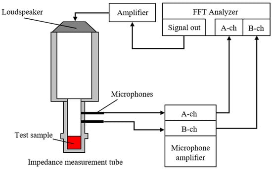
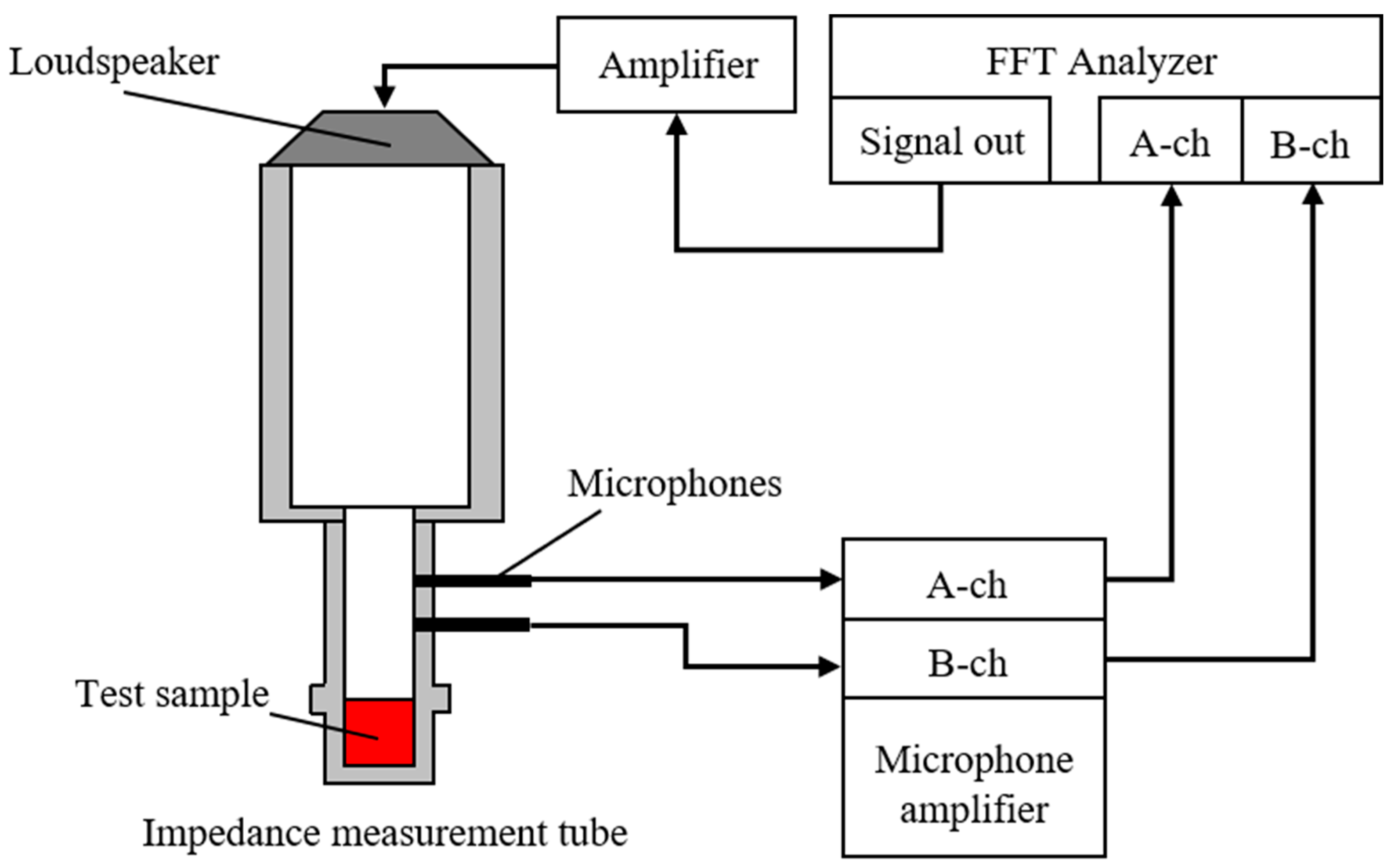
A Brüel & Kjær (Narum, Denmark) Type 4206 two-microphone impedance measurement tube was used to measure the sound absorption coefficient. Figure 1 presents a schematic of the experimental apparatus. Samples were mounted in an impedance tube, and a sinusoidal signal generated by the FFT analyzer (Yokohama, Japan) was used to drive a loudspeaker, introducing sound waves into the tube. The transfer function between the sound pressures measured by two microphones installed on the tube was then obtained using the FFT analyzer. The measured transfer function was used to calculate the normal-incidence sound absorption coefficient in accordance with ISO 10534-2 [13]. The ventilation resistance of the glass wool was measured using an air permeability tester (KES-F8-AP1, Kato Tech Co., Ltd., Kyoto, Japan). A constant volume velocity of air was passed through the specimen, with the flow alternately discharged/drawn in opposite directions. The ventilation resistance R_g was determined from the resulting pressure drop.

Figure 1. Schematic of the experimental apparatus for absorption coefficient measurement.

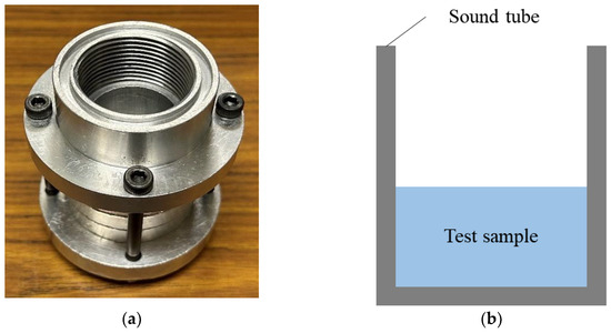
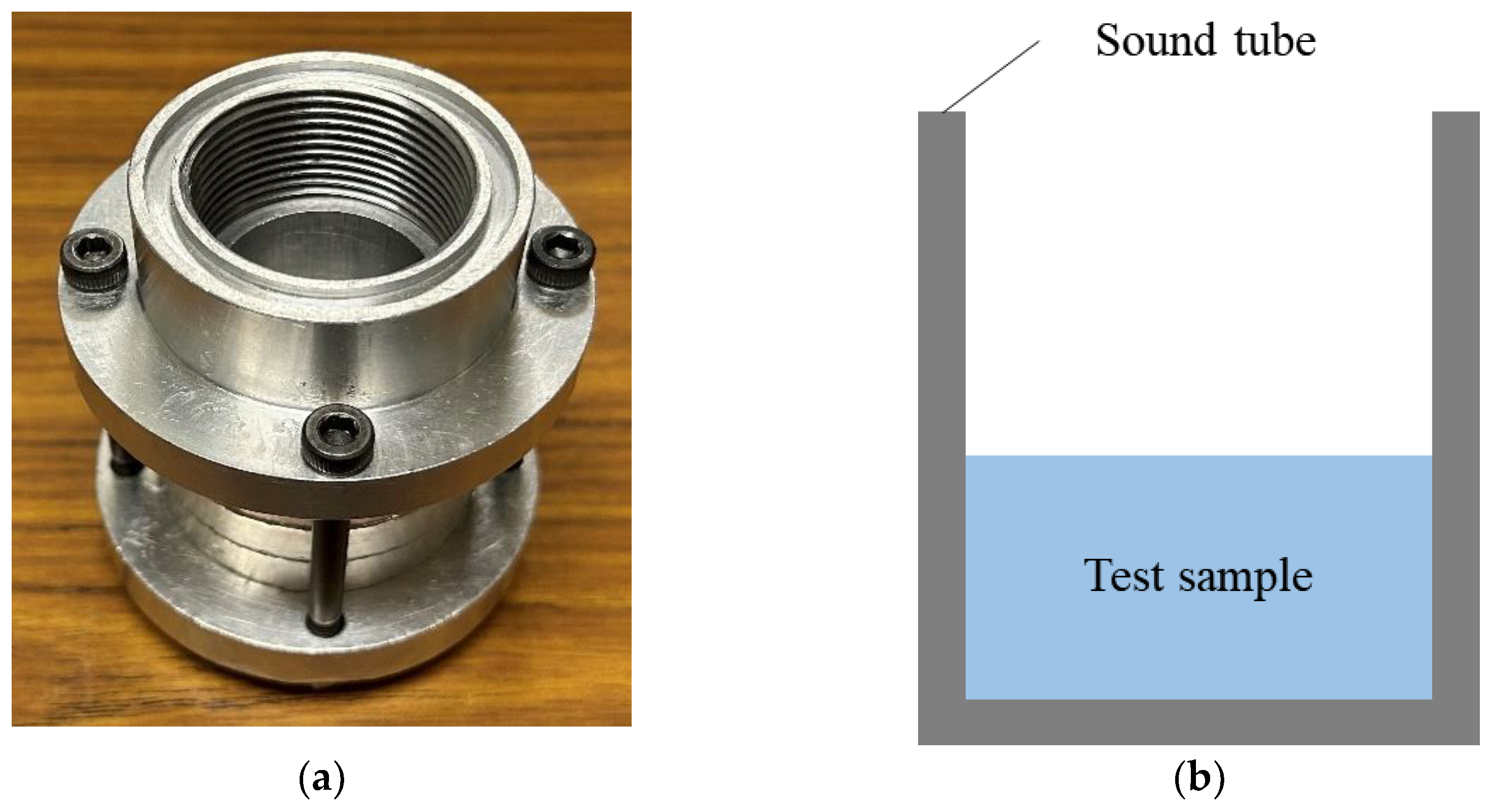
Figure 2a,b show photographs and a schematic of the sample holder. The sample holder was made of aluminum alloy. The upper frequency limit for plane-wave propagation in an impedance tube depends on its inner diameter; the sample holder used in this study had an inner diameter of 29 mm, giving a usable frequency range of 500–6400 Hz. The input voltage of the signal supplied to the loudspeaker was 0.2 V.

Figure 2. (a) Photograph of the sample tube and (b) schematic of the sample tube.

2.2. Samples Used for Measurement

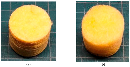
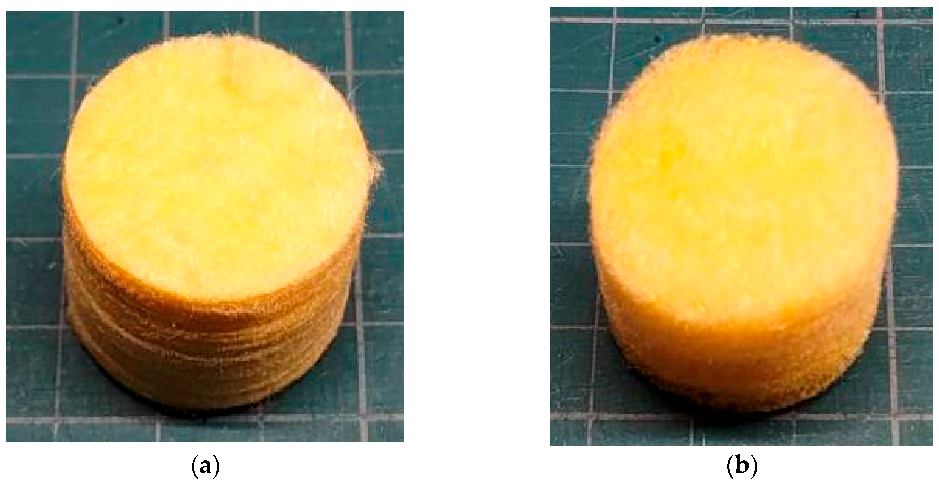
Figure 3a,b show photographs of the 96K and 32K glass wool samples used. The samples were cut to a diameter of 29 mm, corresponding to the inner diameter of the sample holder. Table 1 summarizes the specifications of each material. To ensure redundancy in the sound absorption measurements, six samples were prepared, representing three different specimen thicknesses. The glass wool was manufactured by MAG-ISOVER Co., Ltd. (Tokyo, Japan) using the centrifugal method. The bulk density was measured, whereas the true density was calculated using the standard density of glass (2.5 g/cm³). The ventilation resistance R_g was obtained experimentally using the air permeability tester, and the flow resistivity σ_g was calculated by dividing R_g by the glass wool thickness t_g.

Figure 3. Test samples: (a) 96K glass wool; (b) 32K glass wool.

Table 1. Material specifications.

	Thickness ${\mathit{t}}_{\mathit{g}}$ (mm)	Bulk Density ${\mathit{\rho }}_{\mathit{b}}$ (kg/m3)	True Density ${\mathit{\rho }}_{\mathit{t}}$ (g/cm3)	Porosity $\mathit{n}$	Measured Tortuosity ${\mathit{\alpha }}_{\mathit{\infty }}$	Fiber Diameter (µm) (σ: Standard Deviation)	Ventilation Resistance ${\mathit{R}}_{\mathit{g}}$ (kPa∙s/m)	Flow Resistivity ${\mathit{\sigma }}_{\mathit{g}}$ (kPa∙s/m2)
Glass wool 96K	10	97.5	2.5	0.961	1.14	10.7 (σ: 2.55)	0.554	55.40
	20						1.130	56.48
	40						1.744	43.59
Glass wool 32K	10	31.7	2.5	0.987	1.09	10.8 (σ: 3.10)	0.143	14.25
	20						0.573	28.63
	40						0.920	23.00

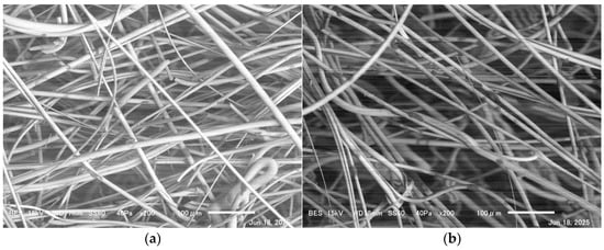
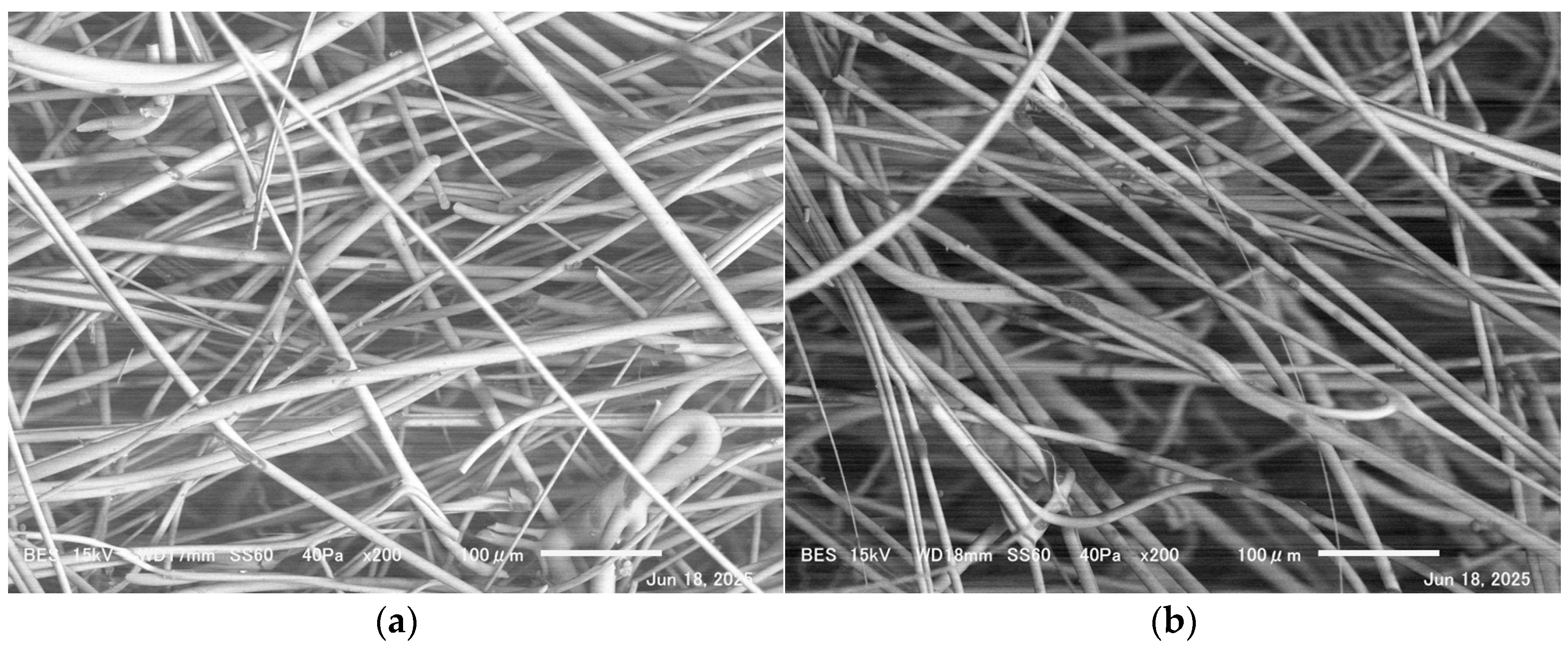
Fiber diameter measurements were performed using a scanning electron microscope (SEM). Figure 4a,b show SEM images of the glass wool. The mean fiber diameters obtained were 10.9 and 10.7 μm for the 96K and 32K glass wools, respectively. The standard deviations of the fiber diameters are shown in Table 1.

Figure 4. Glass wool fibers observed using SEM: (a) 96K glass wool; (b) 32K glass wool.

2.3. Tortuosity Measurement Results

Tortuosity of glass wool was measured using an experimental method involving an ultrasonic sensor [14]. In general, the tortuosity ${\alpha }_{\mathrm{\infty }}$ can be expressed in terms of the speed of sound in air $c_0$ and the apparent speed of sound within the porous structure $c$ as follows:

$${\alpha }_{\infty }={\left({\displaystyle \frac{c_0}{c}}\right)}^2,$$

(1)

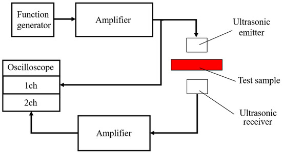
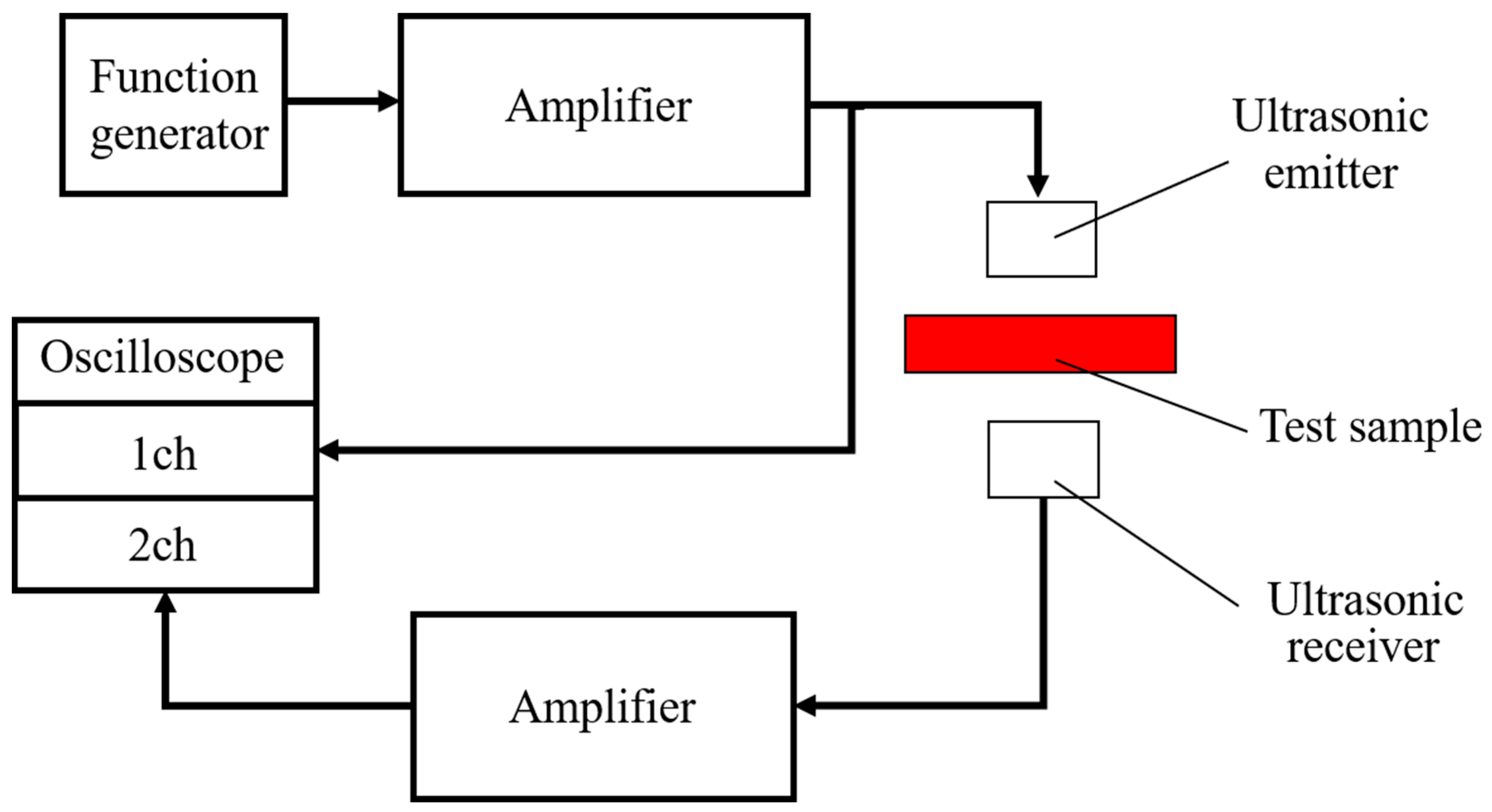
Figure 5 illustrates the apparatus configuration used to measure tortuosity. The measurement system comprises an ultrasonic signal generator, an ultrasonic power amplifier, ultrasonic transmitting and receiving transducers, and an oscilloscope.

Figure 5. Configuration of the apparatus for tortuosity measurement.

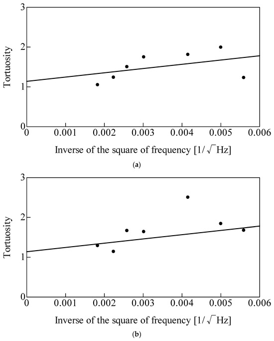
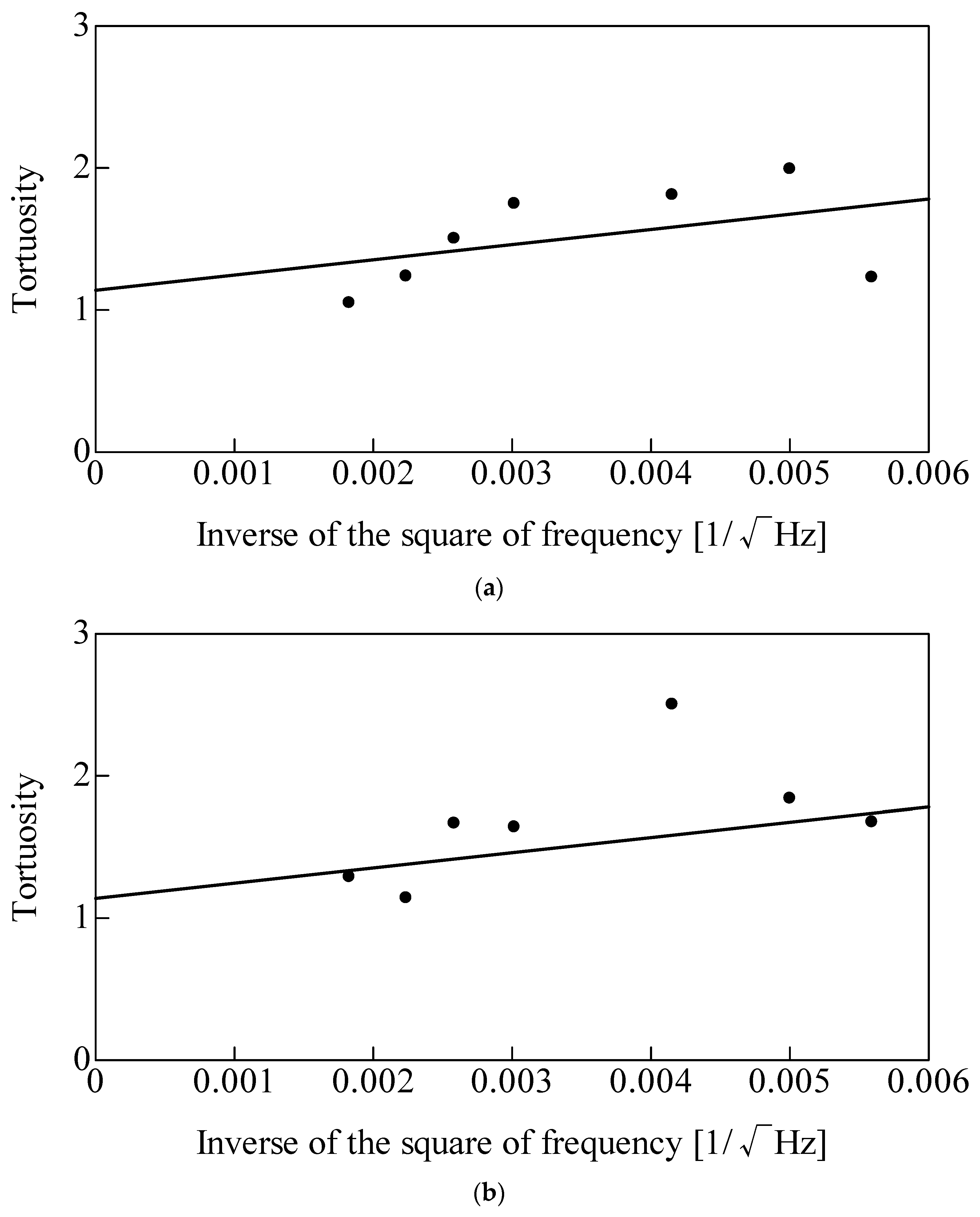
Figure 6 shows the tortuosity measurement results. The y-intercept of the best-fit straight line represents the tortuosity α_∞ for each type of glass wool. The values obtained were α_∞ = 1.14 for the 96K glass wool and α_∞ = 1.09 for the 32K glass wool.

Figure 6. Tortuosity measurement results: (a) 96K glass wool; (b) 32K glass wool.

These measurement results and the estimates derived using the method of du Plessis et al. [15,16] suggest that a tortuosity value of approximately 1.1 can be used for glass wool.

3. Theoretical Estimation

3.1. Nano-CT Scanning

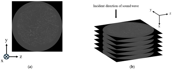
To obtain geometric information on the glass wool fibers, cross-sectional images were acquired using nano-CT scanning. Figure 7a shows an example of the acquired cross-sectional image. The equipment used was the SKYSCAN2214, manufactured by Bruker Corporation (Billerica, MA, USA). Figure 7b presents a schematic illustrating that the tomographic images were acquired as slices in the y–z plane, perpendicular to the direction of sound wave incidence (x-direction). The resolution of the resulting y–z tomographic images was 3960 × 3960, with a spatial resolution of 3 μm. A total of 1666 images were acquired over a 5 mm range in the x-direction.

Figure 7. Glass wool cross-sectional images: (a) typical cross-sectional image of the arbitrary point of the x-direction; (b) schematic of imaging perpendicular to the sound wave incidence direction.

3.2. Image Processing

The images obtained from the CT scans were 8-bit (256-level) greyscale images. To extract the fiber perimeters, the CT images were binarized.

To accurately extract the fiber regions from the images, local binarization was employed. This technique divides an image into small regions and determines a threshold for each region based on its luminance distribution [17]. This approach preserves fine details of the fibers’ shapes while suppressing noise. During local binarization, a sensitivity parameter must be set. Sensitivity was determined by visual inspection to ensure that the fine fiber contours were retained without introducing excessive noise.

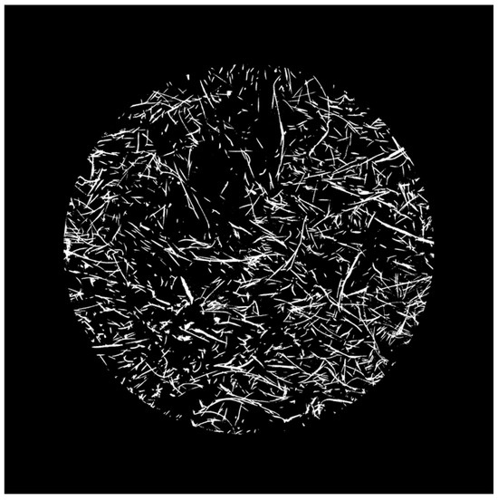
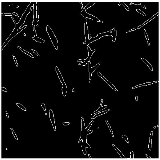
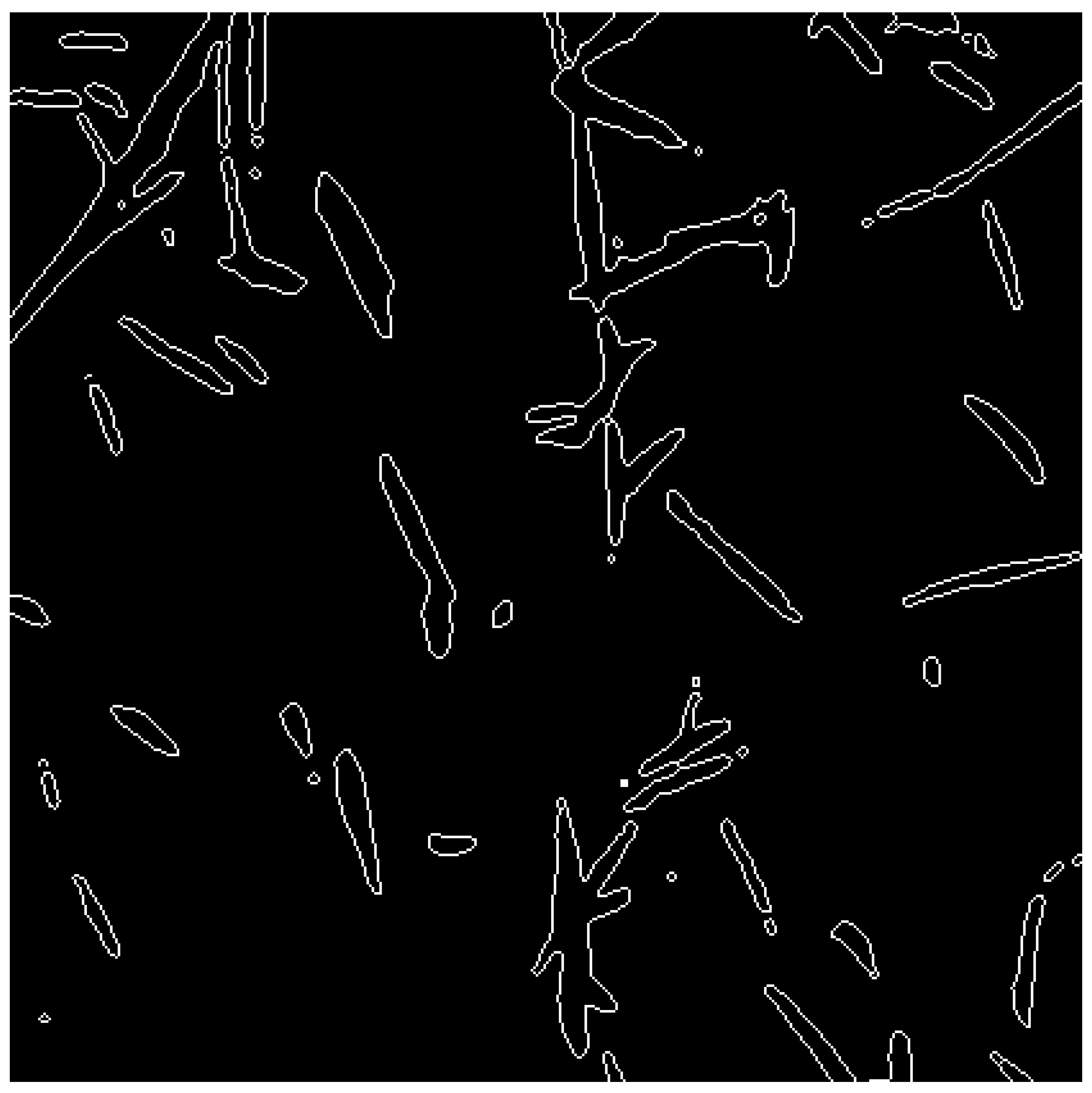
Furthermore, the CT image shown in Figure 7 includes regions surrounding the sample. To restrict the analysis to the region of interest, the image was cropped to a circular area of 3000 pixels centered on the image. Figure 8 shows an example of the binarized and cropped image (sensitivity: 0.57). Following this preprocessing, the Canny edge detection method [18] was employed to obtain fiber perimeters that more closely approximate the actual structure. Figure 9 shows an enlarged view of the image after edge extraction. As the methodology is consistent with previous studies [19,20,21,22], a detailed overview of the method is omitted. Because the number of CT images is very large, the dataset inherently contains redundancy.

Figure 8. Binarized image (sensitivity: 0.57).

Figure 9. Edge extraction using the Canny edge detection method.

3.3. Surface Area Correction Considering Fiber Inclinations

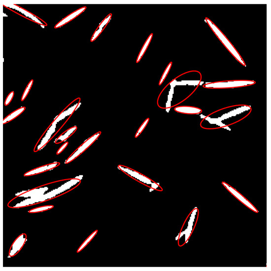
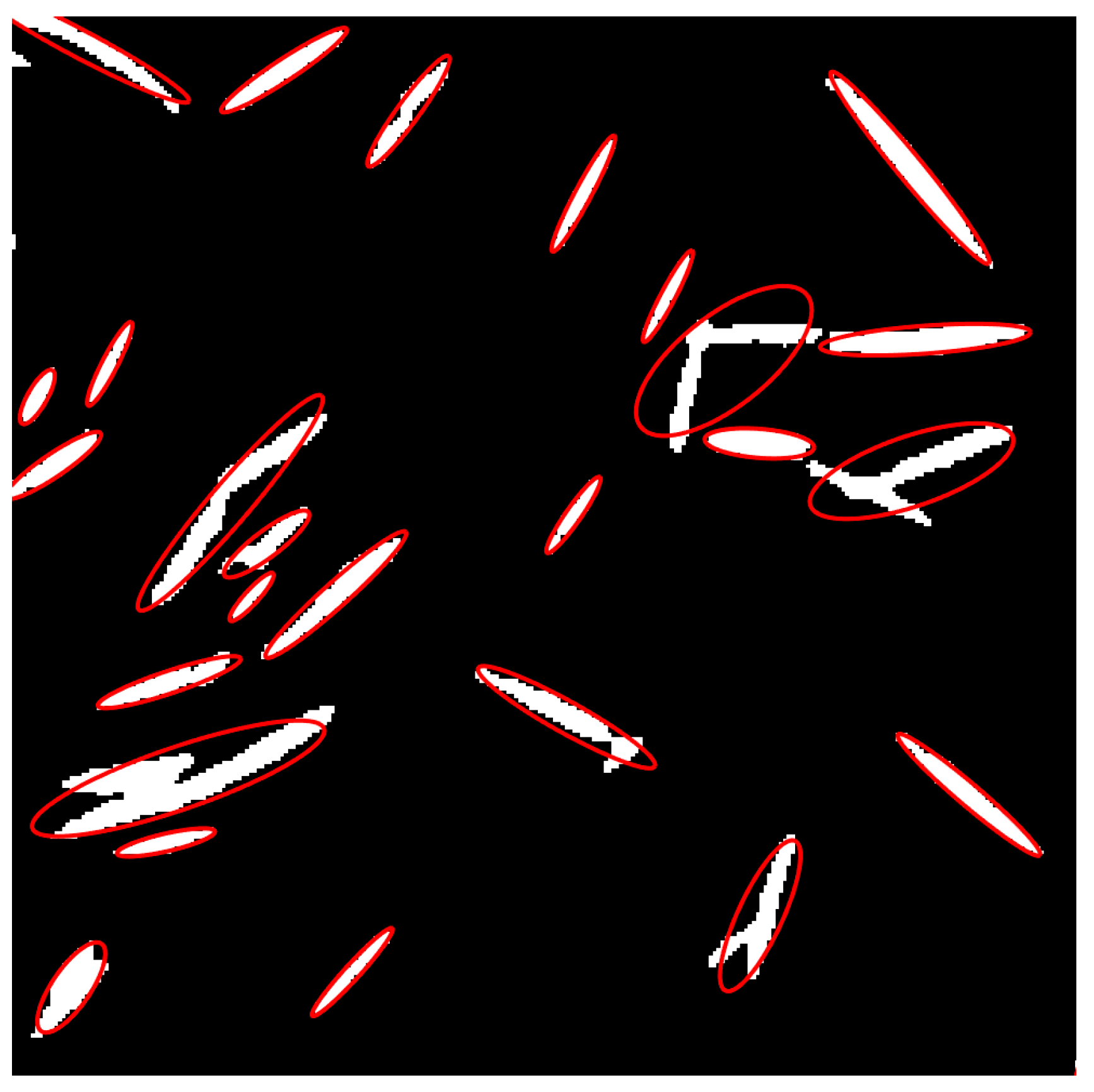
Observations of CT scan images reveal that the fiber contours appear elliptical, indicating that the fibers are inclined relative to the image plane.

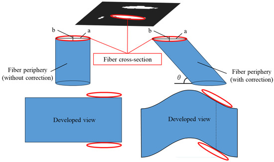
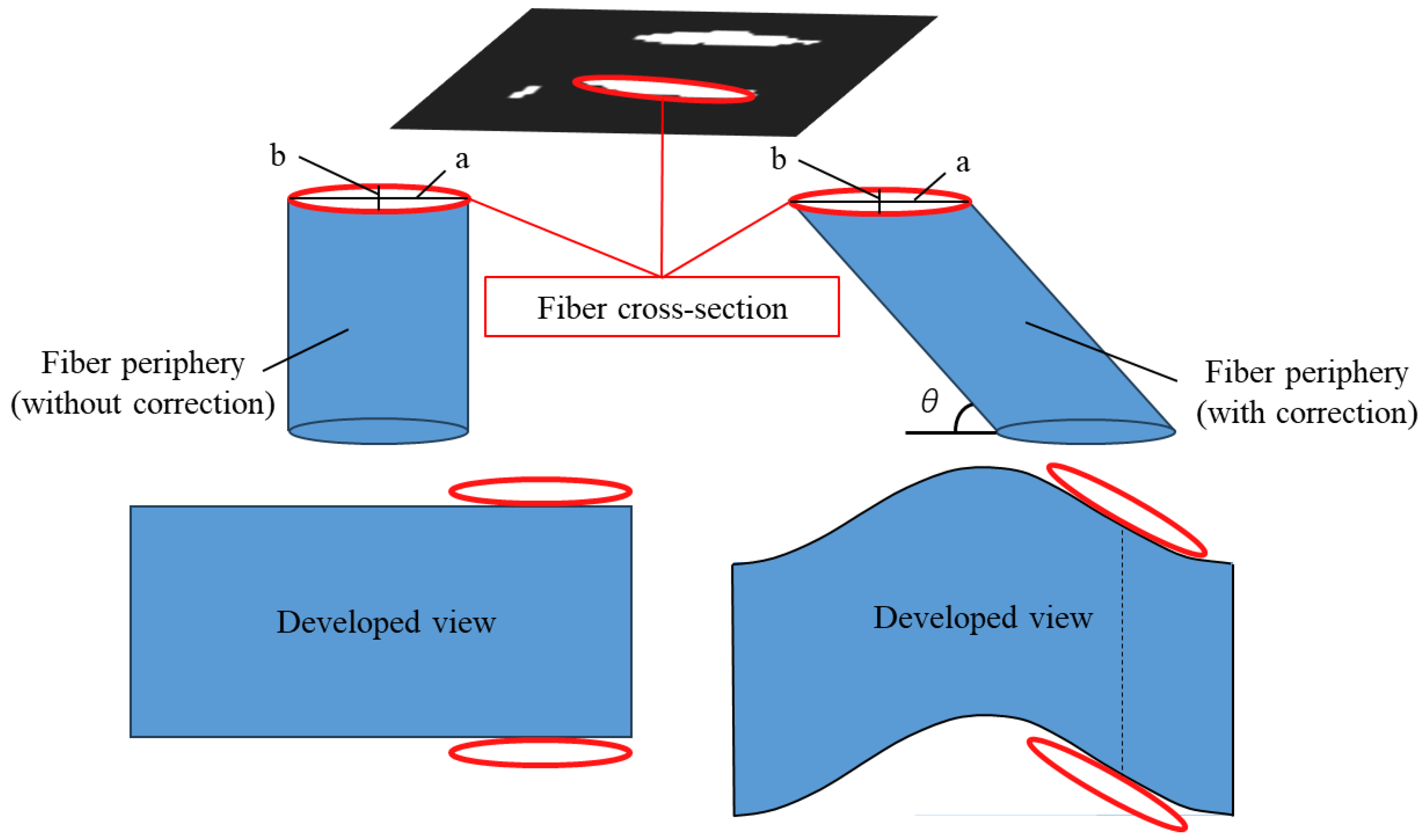
In the example shown on the left side of Figure 10, the surface area of the fiber side was calculated by multiplying the perimeter of the fiber cross-section by the image pitch (fiber length). However, as illustrated on the right side of Figure 10, the surface area of an inclined fiber is as shown in the developed diagram. Therefore, the surface area calculated in the example shown on the left side of Figure 10 is an underestimate. Consequently, the surface area must be corrected to account for the fiber’s inclination.

Figure 10. Schematic of the fiber periphery and its developed view ((left): without surface area correction; (right): with correction).

Therefore, the fiber cross-sections in the tomographic images were approximated as ellipses, and the fiber inclination angle was determined from the ellipticity to derive a surface area correction factor [23]. The regionprops function in MATLAB (R2025b) was used for elliptical approximation. Figure 11 shows an image where fiber cross-sections are approximated as ellipses. In some cases, the fitting process incorrectly merges multiple fibers into a single cross-section. To prevent such misidentified ellipses from affecting the statistical analysis, ellipses with a minor axis significantly larger than the fiber diameter were excluded. The eccentricity (e) of the approximated ellipse is expressed as follows.

$$e=\sqrt{1-{\left({\displaystyle \frac{b}{a}}\right)}^2,}$$

(2)

where a is the major axis and b is the minor axis of the ellipse.

Figure 11. Ellipse approximation of fiber cross-section.

Therefore, the perimeter (L) of the ellipse is expressed using the complete elliptic integral of the second kind (E(e)) as follows:

$$L=4aE\left(e\right),$$

(3)

where

$$E\left(e\right)={\int }_0^{{\displaystyle \frac{\pi }{2}}}\sqrt{1-e^2{sin}^2\varphi }d\varphi .$$

(4)

Furthermore, assuming a circular fiber cross-section, the angle of inclination (θ) of the fiber relative to the image plane can be determined from the aspect ratio of the ellipse as follows:

$$\theta ={\mathrm{s}\mathrm{i}\mathrm{n}}^{-1}\left({\displaystyle \frac{b}{a}}\right).$$

(5)

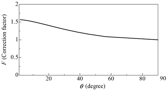
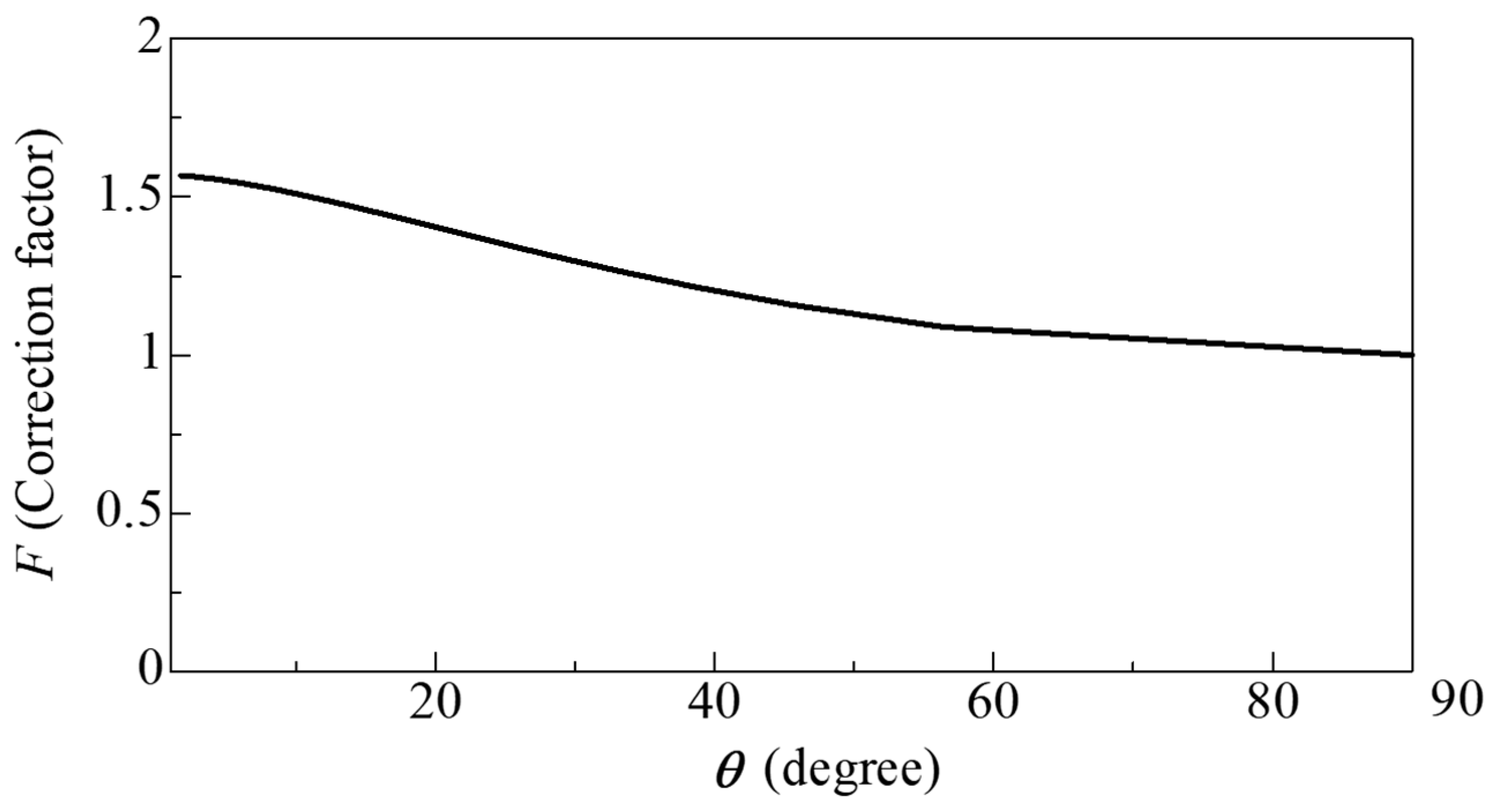
From the above, the surface area correction factor F, which accounts for the increase in surface area due to fiber inclination, is given by

$$F={\displaystyle \frac{b\pi }{L\mathrm{s}\mathrm{i}\mathrm{n}\theta }}.$$

(6)

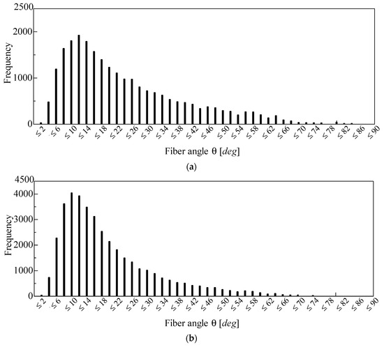
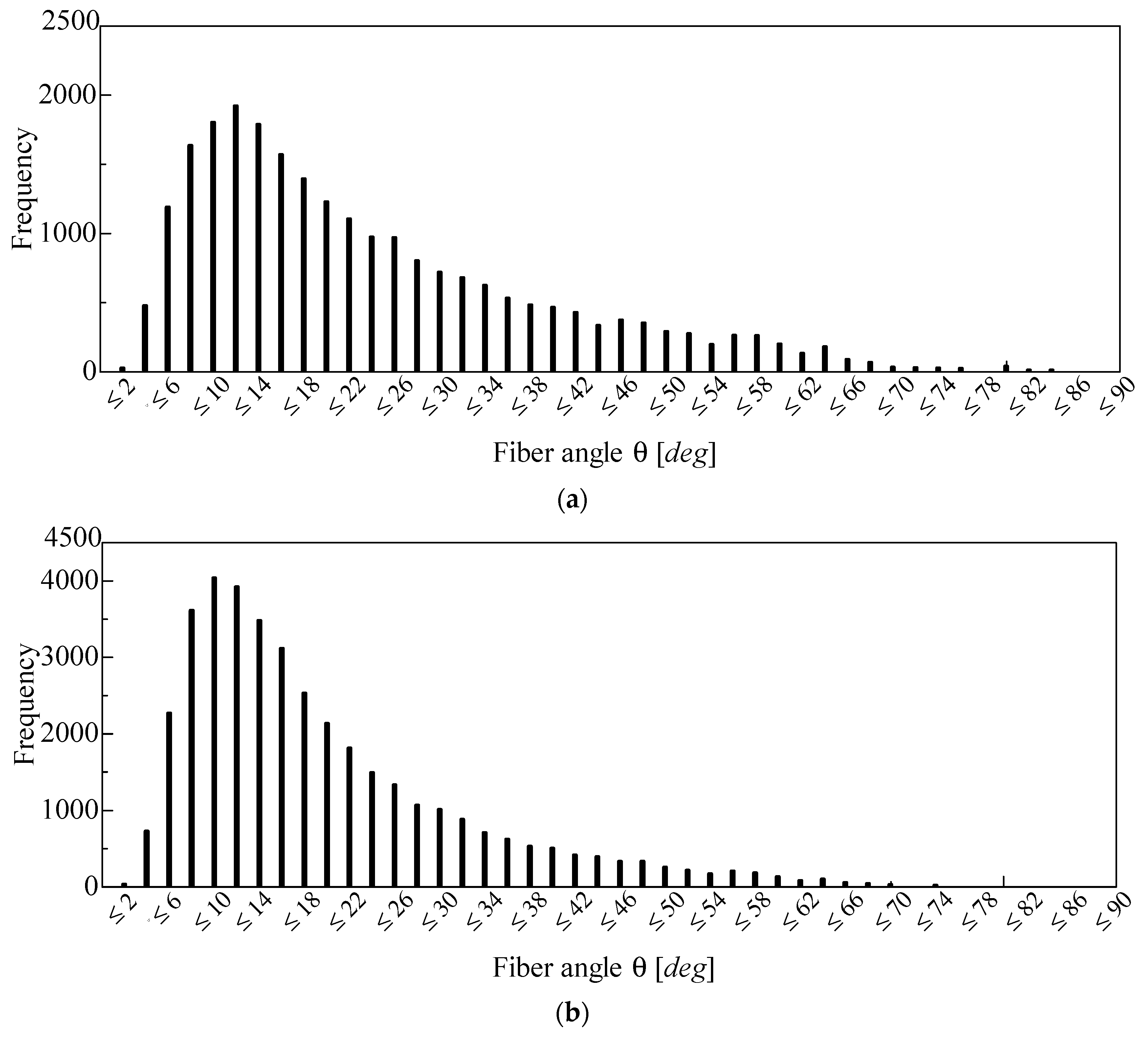
Figure 12 shows the distribution of fiber inclination angles obtained using Equation (4). Figure 12a shows the inclination angles detected from the CT image of the 96K glass wool, while Figure 12b shows those detected from the CT image of the 32K glass wool. Furthermore, the median and mean values in Figure 12a are 14.2° and 17.8°, respectively, whereas those in Figure 12b are 18.7° and 23.2°, respectively. In this study, the correction factor corresponding to the median value of θ was used.

Figure 12. Frequency distribution of fiber angles detected from the CT image of the (a) 96K glass wool and (b) 32K glass wool.

Figure 13 shows the relationship between F (obtained from Equation (6)) and θ (as shown in Equation (5)). As θ decreased, F asymptotically approached π/2 mathematically. In other words, when the fiber was parallel to the image plane, the surface area of the fiber was maximized. Conversely, as θ increased, F decreased monotonically; naturally, when θ = 90°, F = 1.

Figure 13. Relationship between the correction factor F and the inclination angle θ.

3.4. Approximation to Clearance Between Two Planes

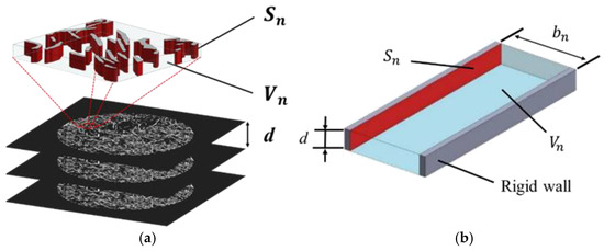
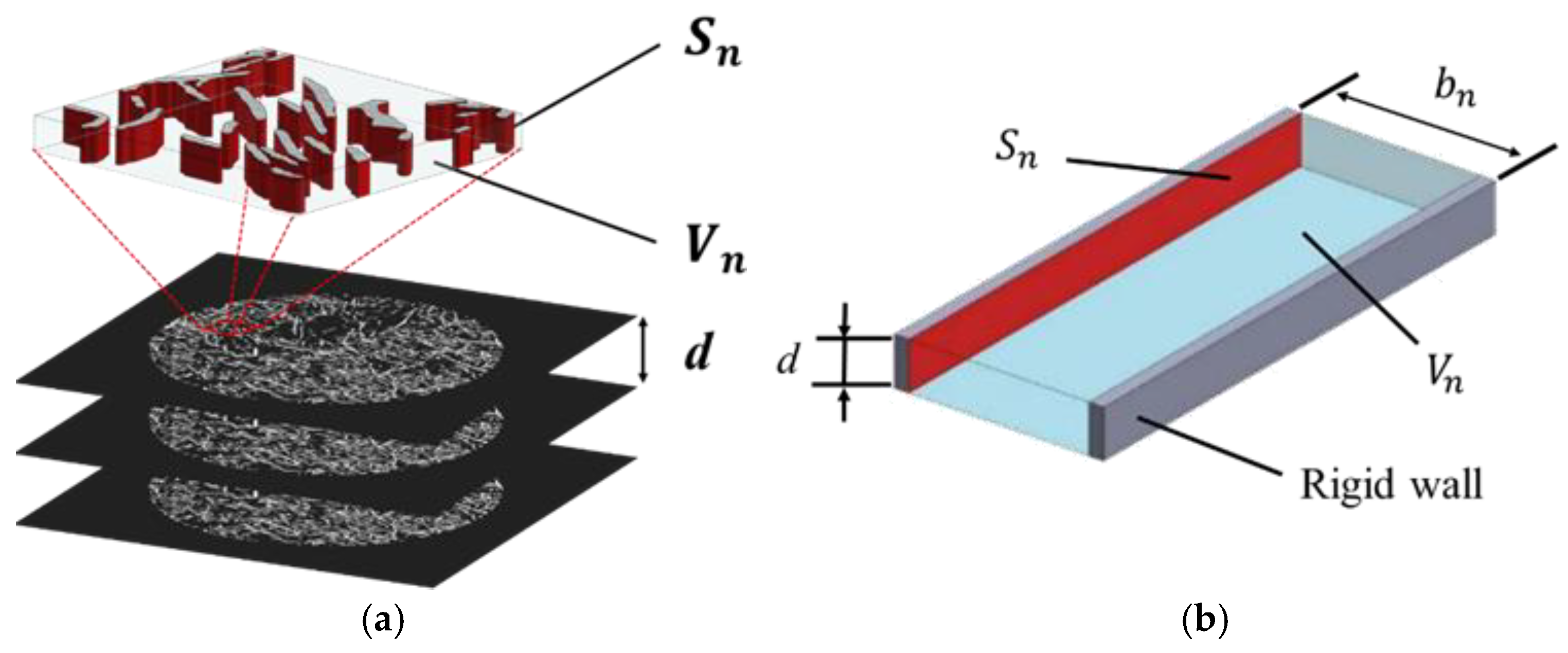
Based on the fiber cross-sectional perimeter obtained from the images, the voids between fibers were approximated as the clearance between two planes. Figure 14 schematically illustrates the configurations before and after the two-plane approximation. The fiber surface area S_n was obtained by multiplying the total fiber perimeter calculated in Section 3.2 by the image pitch d and the inclination correction factor F derived in the previous section. However, it is known that in CT images, the void volume is underestimated because of the partial-volume effect [24]. Therefore, in this study, the void volume was calculated from the porosity (n) of the actual sample, expressed as follows using the true density ρ_t and the bulk density ρ_b of the sample:

$$n=1-{\displaystyle \frac{{\rho }_b}{{\rho }_t}}.$$

(7)

Figure 14. Fiber surface area and void volume: (a) cross-sectional image of an arbitrary point in the x-direction; (b) two-plane modeling.

Consequently, the void volume (V_n) can be calculated using the sample volume (V), as shown in the following equation:

$$V_n=n\times V.$$

(8)

For a single tomographic image, the thickness of the clearance between the two planes shown in Figure 14b (b_n) can be calculated as follows.

$$b_n={\displaystyle \frac{2V_n}{S_n}}.$$

(9)

3.5. Propagation Constant and Characteristic Impedance

The propagation constant and characteristic impedance, accounting for the attenuation of sound waves in the clearance between two planes, were derived. For propagation constant and characteristic impedance formulations that consider viscous air effects within a tube, prior studies include those by Tijdeman [25] and Stinson [26] for circular tubes, Stinson [27] for tubes with cross-sections such as equilateral triangles, and Beltman [28] for rectangular tubes. In addition, Allard [29] presented an analysis accounting for tortuosity.

In this study, the methods proposed by Stinson [27] and Allard [29] were employed [19,20,21,22]. Using three-dimensional (3D) analysis based on the Navier–Stokes equations and other formulations, the propagation constant γ and characteristic impedance Z_c are expressed in terms of the effective density ρ_s and compressibility C_s. Here, the tortuosity ${\alpha }_{\mathrm{\infty }}$ is considered by multiplying it by the effective density [27]:

$$\gamma =j\omega \sqrt{{\alpha }_{\mathrm{\infty }}{\rho }_s{C}_s},$$

(10)

$$Z_c=\sqrt{{\displaystyle \frac{{\alpha }_{\mathrm{\infty }}{\rho }_s}{C_s}}}.$$

(11)

Based on the one-dimensional wave equation, the sound absorption coefficient was derived using the transfer matrix method for sound pressure and volume velocity. The details of the derivation have been omitted as they are identical to those in previous studies [17,18,19,20].

4. Experimental and Theoretical Values

4.1. Investigation of the Optimal Sensitivity for Binarization

As discussed in Section 3.2, to accurately extract the fiber perimeter, the fiber’s outline must be preserved while suppressing the generation of excessive noise. Therefore, the local binarization sensitivity must be appropriately set.

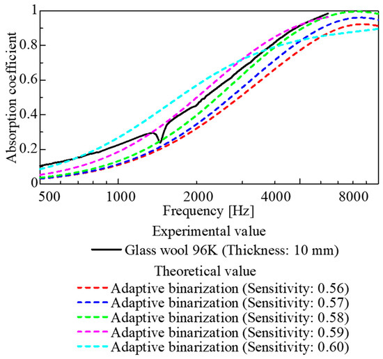
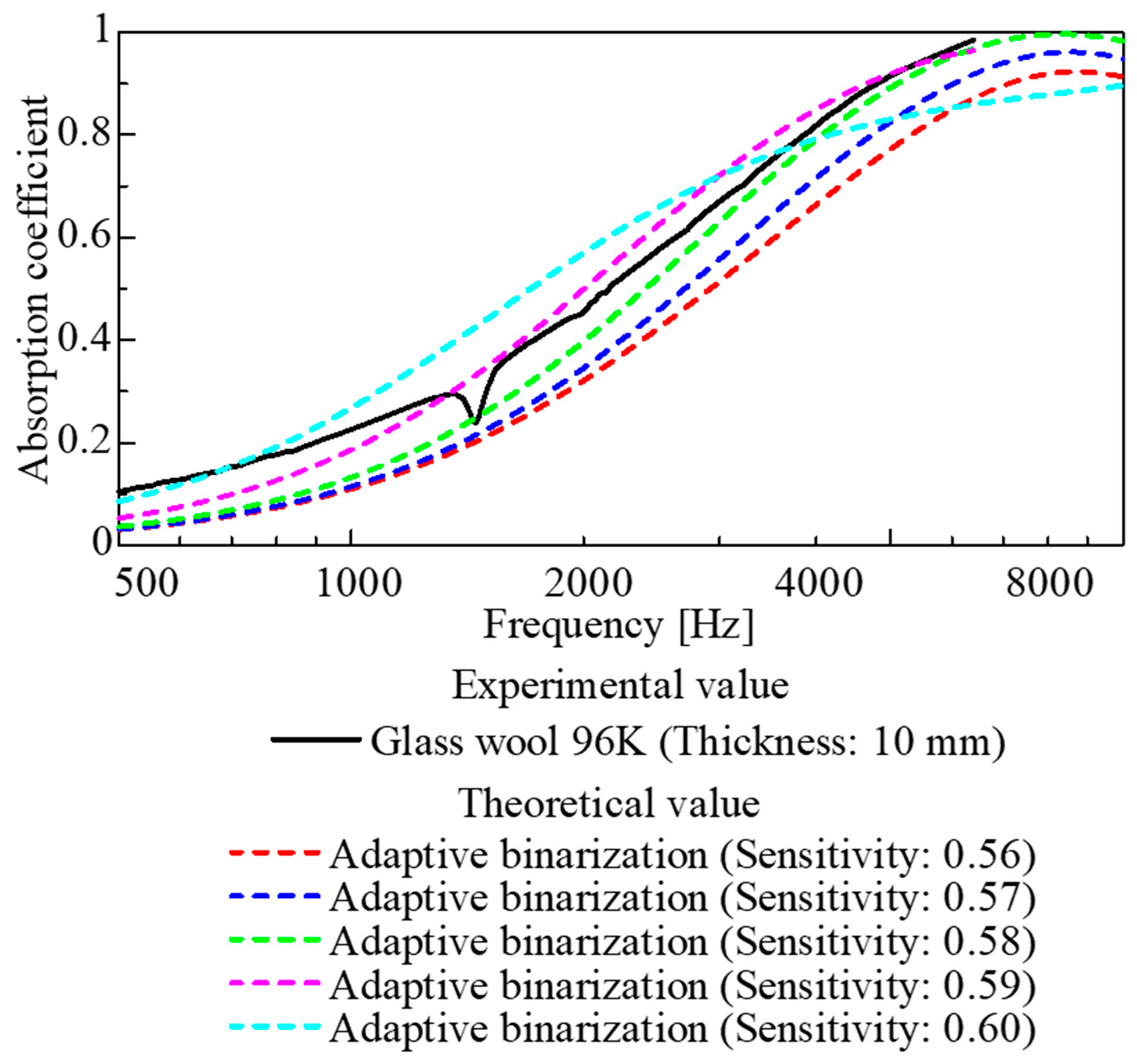
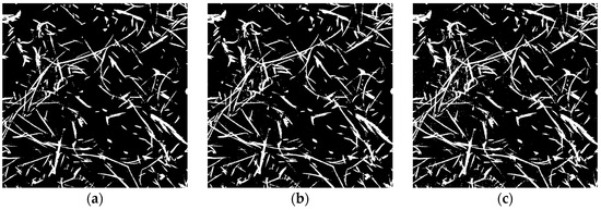
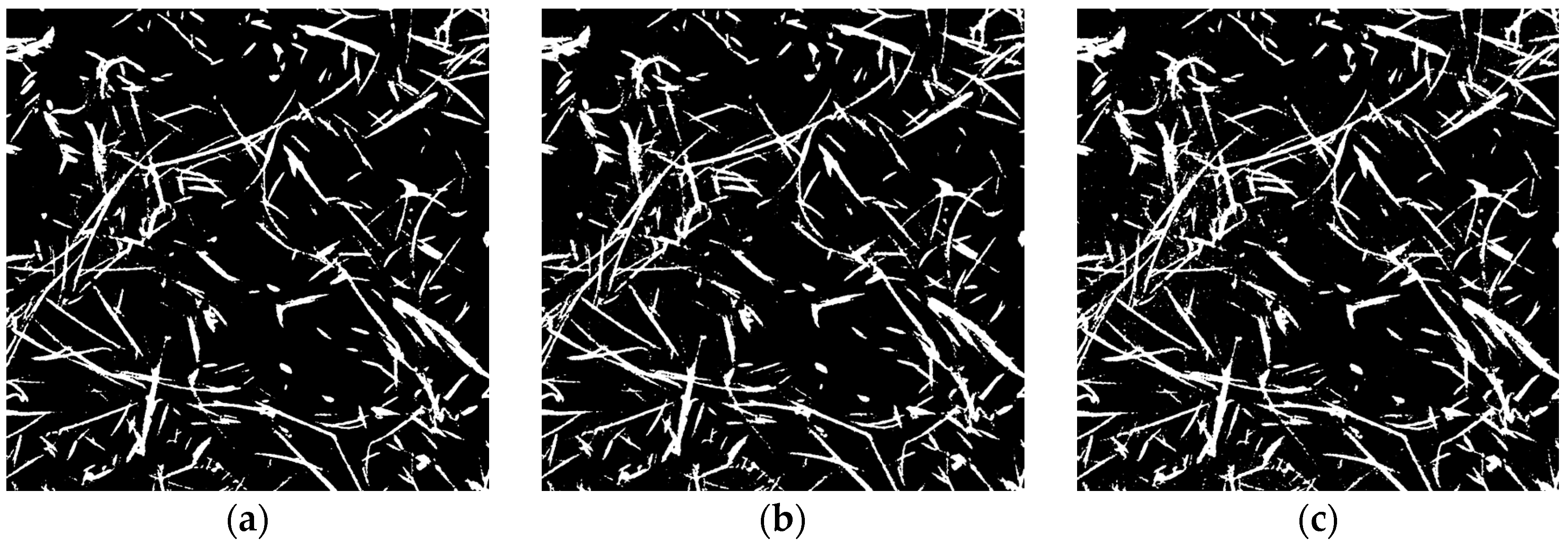
Figure 15 shows the results of a parameter study where the sensitivity of local binarization was varied for the CT images of the 96K glass wool. Meanwhile, Figure 16a–c show binarized images for each sensitivity setting.

Figure 15. Sound absorption coefficient for each binarization sensitivity.

Figure 16. Binarized images at various sensitivities: (a) 0.56, (b) 0.57; (c) 0.58.

When the sensitivity was too low (Figure 16a), although there was little noise, some fibers appeared to be missing. Consequently, the extracted perimeter was underestimated, resulting in a generally lower theoretical value for the sound absorption coefficient. Conversely, when the sensitivity was too high (Figure 16c), excessive noise remained; consequently, although the theoretical values were close to the experimental values at frequencies of 3 kHz and above, the general shape of the sound absorption curve tended to differ slightly from the experimental data.

As shown in Figure 16b, although the theoretical values obtained using a binary image with a sensitivity of 0.57 did not come as close to the experimental values as those with a sensitivity of 0.58 for sound absorption coefficients above 3 kHz, the general shape of the sound absorption curve was similar to that of the experimental data.

Furthermore, the agreement between the theoretical and experimental values was quantitatively assessed using the root mean square error (RMSE) defined in Equation (12).

$$\mathrm{R}\mathrm{M}\mathrm{S}\mathrm{E}=\sqrt{{\displaystyle \frac{1}{N}}{\displaystyle \sum _{i=1}^N}{\left(X_{theo}\left(f_i\right)-X_{exp}\left(f_i\right)\right)}^2}.$$

(12)

Here, the theoretical and experimental values at frequency $f_i$ are denoted by $X_{theo}\left(f_i\right)$ and $X_{exp}\left(f_i\right)$, respectively, and N is the number of frequency points used in the evaluation.

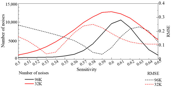
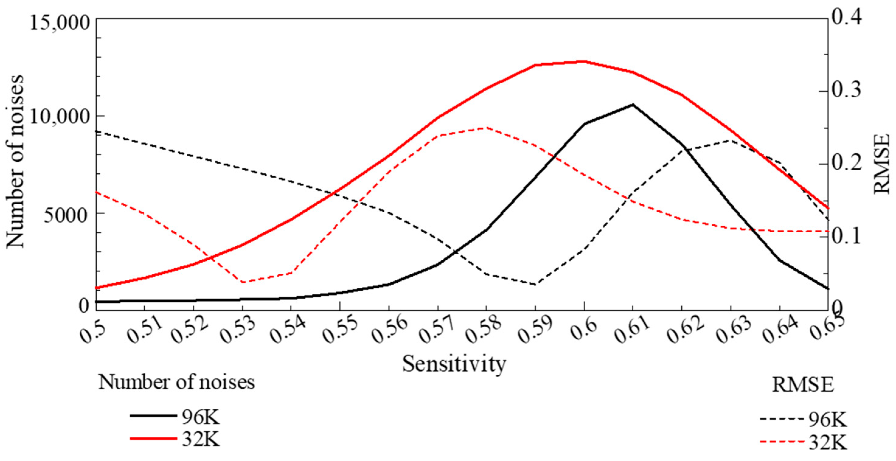
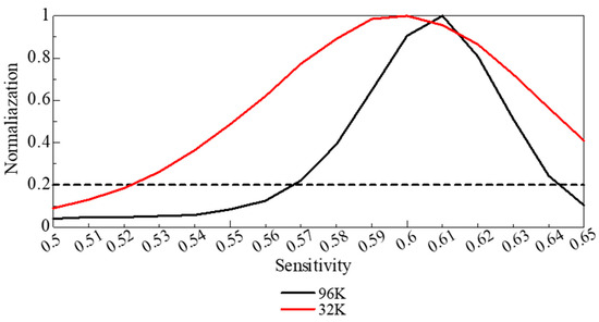
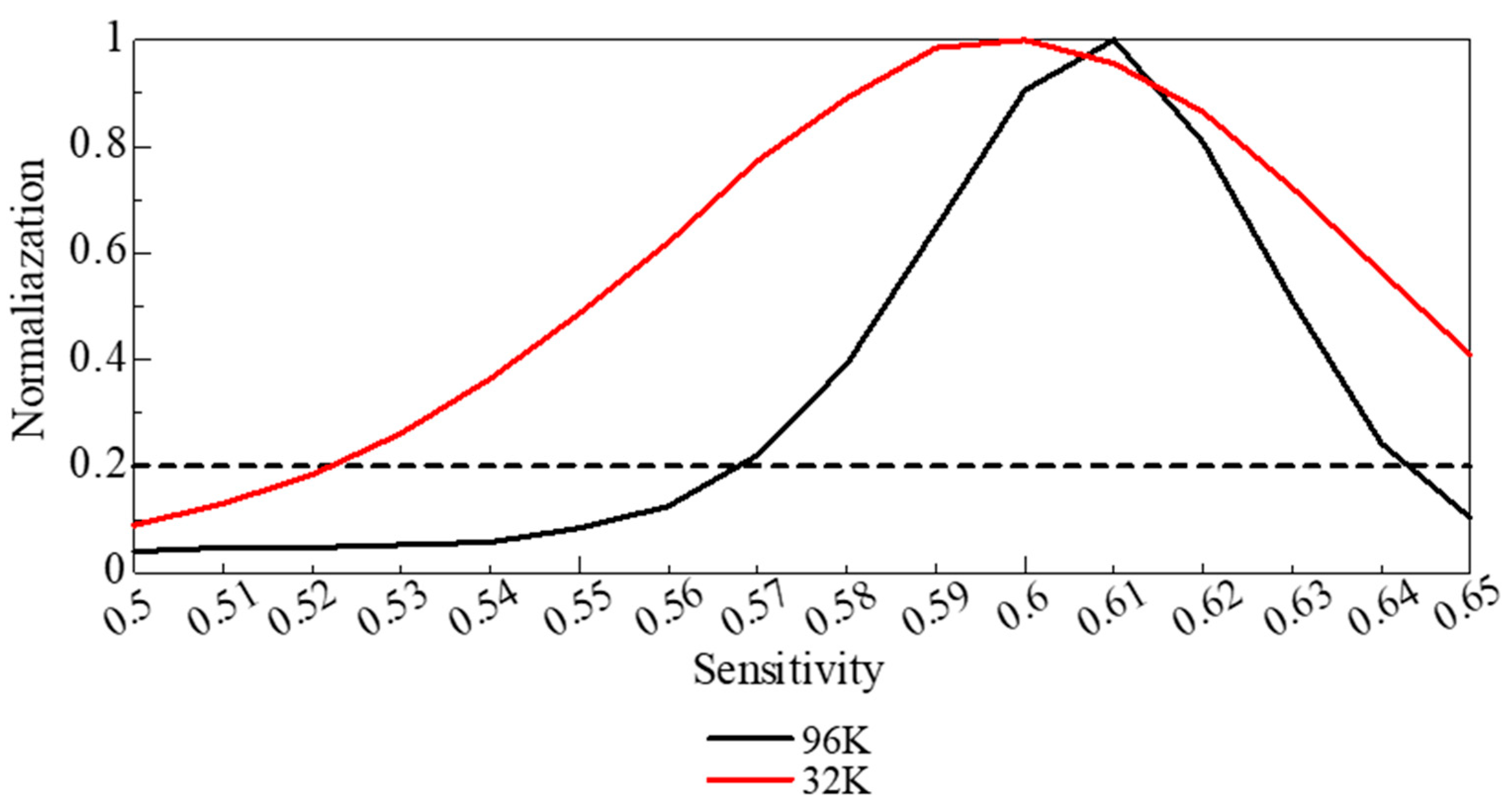
Figure 17 shows the relationship between RMSE at each binarization sensitivity and the number of white pixels smaller than 5 pixels in the binarized image, which are counted as noise. Figure 18 shows the corresponding noise counts normalized by their maximum value. The sensitivity at which the RMSE was minimal, the images contained excessive noise, leading to an overestimation of the fiber cross-sectional area. By contrast, sensitivities for which the normalized noise count was ~0.2 generally agreed with the optimal values obtained by visual inspection. Therefore, herein, the binarization sensitivity was selected by jointly considering the noise-count behavior, the visual validity of the binarized images, and the RMSE of the sound absorption coefficient curve.

Figure 17. Number of noise counts (white regions smaller than 5 pixels) and RMSE as a function of binarization sensitivity. At the sensitivity corresponding to the minimum RMSE, the fiber cross-sectional area is overestimated.

Figure 18. Relationship between sensitivity and normalized noise count; the trade-off between noise reduction and loss of image information occurs at a normalized noise count of ~0.2.

Given these results and considering the accuracy of fiber contour extraction, noise tolerance, and the general shape of the sound absorption curve, a sensitivity of 0.57 was considered as the optimal binarization threshold.

4.2. Comparison of Experimental and Theoretical Values

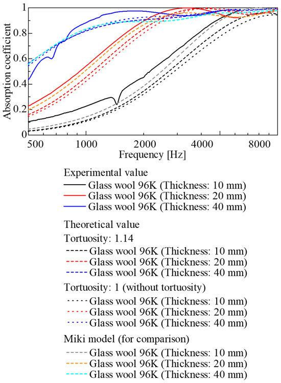
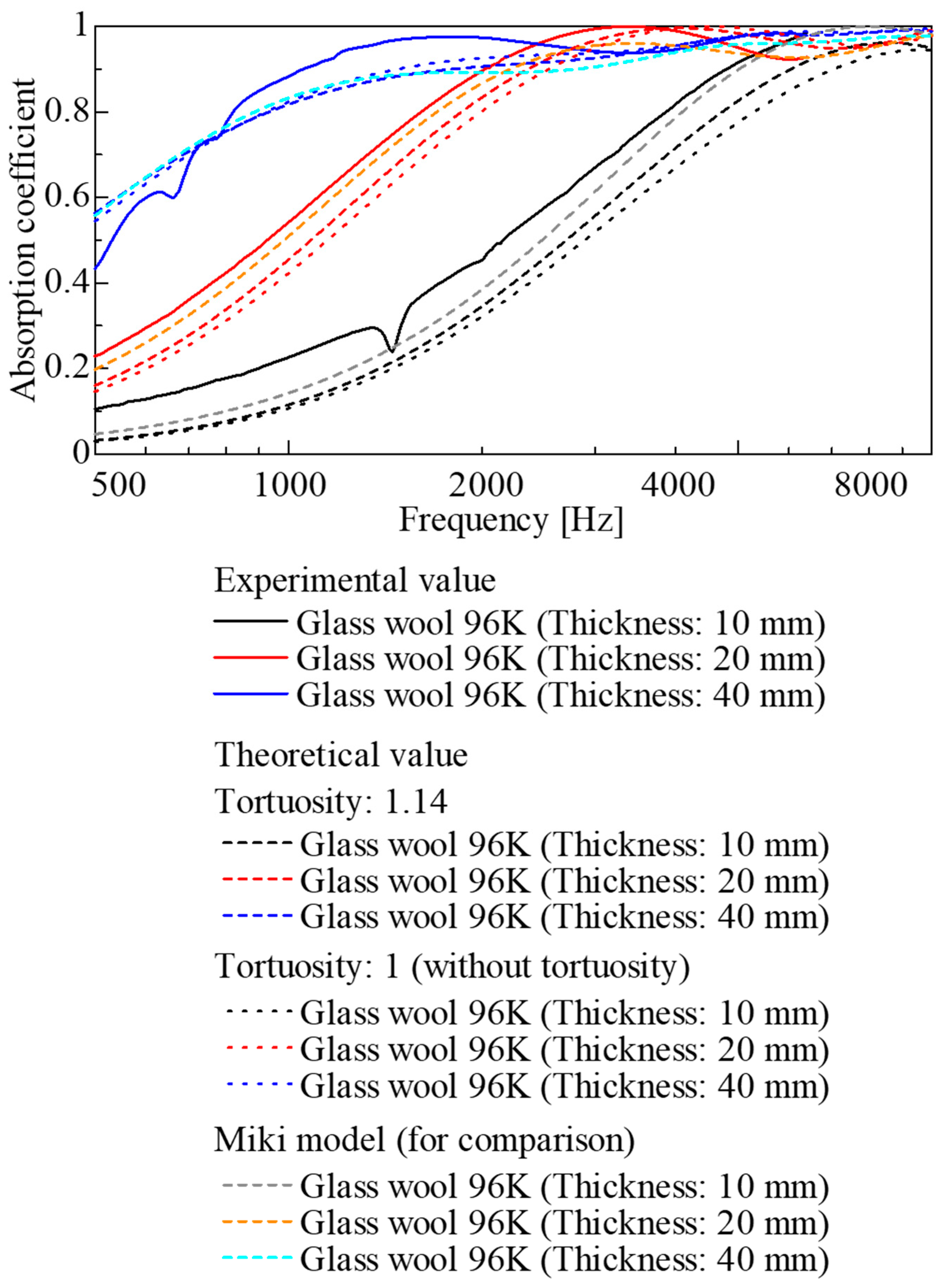
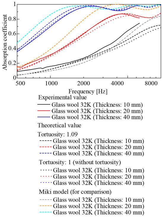
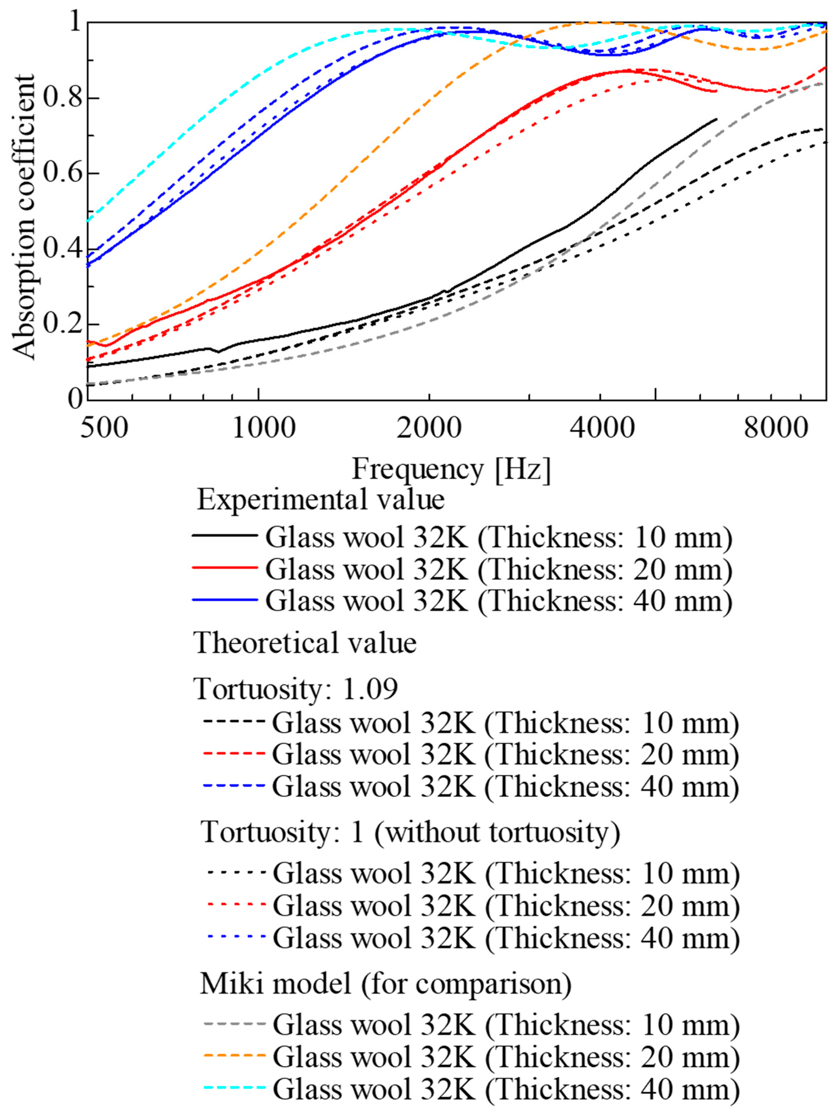
The experimental and theoretical sound absorption coefficients were compared for each sample. The results for the 96K glass wool are shown in Figure 19, and those for the 32K glass wool are presented in Figure 20. The theoretical values are shown as dashed lines, accounting for the tortuosity determined through measurement, and as dotted lines, assuming a tortuosity of 1. For comparison, conventional theoretical values derived from the Miki model [9] based on ventilation resistance are also shown in Figure 19 and Figure 20. The experimental values, theoretical values, and those derived from the Miki model are in good agreement.

Figure 19. Comparison of experimental and theoretical sound absorption coefficients (96K glass wool).

Figure 20. Comparison of experimental and theoretical sound absorption coefficients (32K glass wool).

For the 96K glass wool (Figure 19), although the theoretical values followed the trend of the experimental values for each sample thickness, the theoretical values were lower than the experimental values across a wide frequency range for all sample thicknesses.

In comparison, for the 32K glass wool (Figure 20), whereas good agreement between the experimental and theoretical values was observed for thicknesses of 20 and 30 mm, a discrepancy between the experimental and theoretical values was observed in the high-frequency range for a thickness of 10 mm. This could be attributed to the influence of the binarization and edge detection accuracy, as explained in the previous section. In other words, residual noise from image processing and errors in perimeter extraction are considered to have introduced errors into the theoretical values.

Furthermore, when comparing results with and without consideration of tortuosity, the difference between the theoretical values was small for both the 96K and 32K glass wool samples across all thicknesses. This could be ascribed to the generally low tortuosity of fibrous materials. Consequently, for such materials, the sound absorption coefficient can be sufficiently predicted using geometric information alone, without explicitly accounting for tortuosity.

To further quantify the agreement between experimental and theoretical values, the RMSE was also calculated for each sample. Table 2 lists the RMSE values for octave bands centered at 500, 1, 2, and 4 kHz.

Table 2. RMSE between experimental and theoretical sound absorption coefficients in each octave band.

	Thickness		500 Hz (353–707 Hz)	1 kHz (707–1414 Hz)	2 kHz (1414–2828 Hz)	4 kHz (2828–5657 Hz)
Glass wool 96K	10	With tortuosity	0.078	0.107	0.113	0.099
		Without tortuosity	0.080	0.116	0.139	0.145
		Miki	0.062	0.080	0.072	0.034
	20	With tortuosity	0.071	0.085	0.060	0.025
		Without tortuosity	0.087	0.117	0.090	0.036
		Miki	0.033	0.032	0.031	0.030
	40	With tortuosity	0.084	0.067	0.063	0.008
		Without tortuosity	0.068	0.058	0.046	0.006
		Miki	0.081	0.056	0.074	0.021
Glass wool 32K	10	With tortuosity	0.049	0.037	0.023	0.093
		Without tortuosity	0.049	0.039	0.037	0.131
		Miki	0.047	0.061	0.066	0.069
	20	With tortuosity	0.044	0.017	0.008	0.010
		Without tortuosity	0.048	0.027	0.041	0.044
		Miki	0.019	0.091	0.186	0.142
	40	With tortuosity	0.028	0.057	0.024	0.018
		Without tortuosity	0.012	0.015	0.003	0.007
		Miki	0.121	0.150	0.043	0.034

First, when tortuosity was considered, the RMSE was generally smaller and the prediction accuracy higher than when tortuosity was neglected.

Moreover, when comparing the tortuosity-based method with the Miki model, the RMSE values were often of similar magnitude. Notably, for the 20 and 40 mm 32K glass wool specimens, the RMSE was smaller when tortuosity was considered than in the Miki model, indicating that the experimental absorption coefficients can be predicted more accurately under these conditions.

4.3. Simulation of Scaling CT Images to 3D Similarity

As described in Section 3.2, the pixel size in the CT images used in this study corresponded to a 3-μm × 3-μm square, and the pitch at which the CT images sliced the object was also 3 μm. Consequently, the resulting voxel size was a 3-μm cube. In other words, the circular region with a diameter of 3000 pixels corresponded to a diameter of 9 mm. When calculating the sound absorption coefficient based on the CT images, all calculations were performed using the voxel size (spatial resolution) described above.

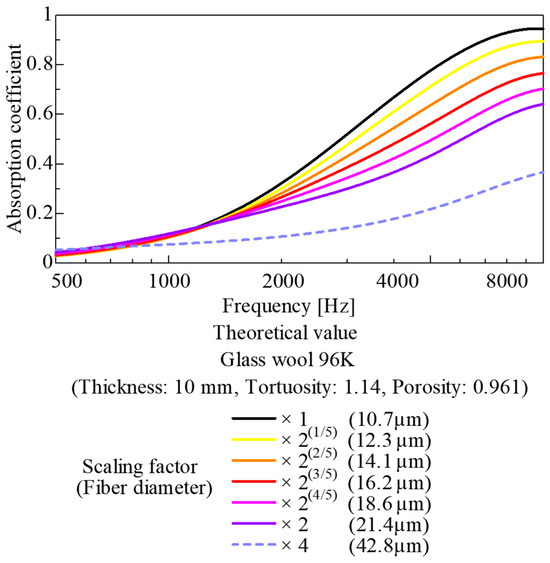
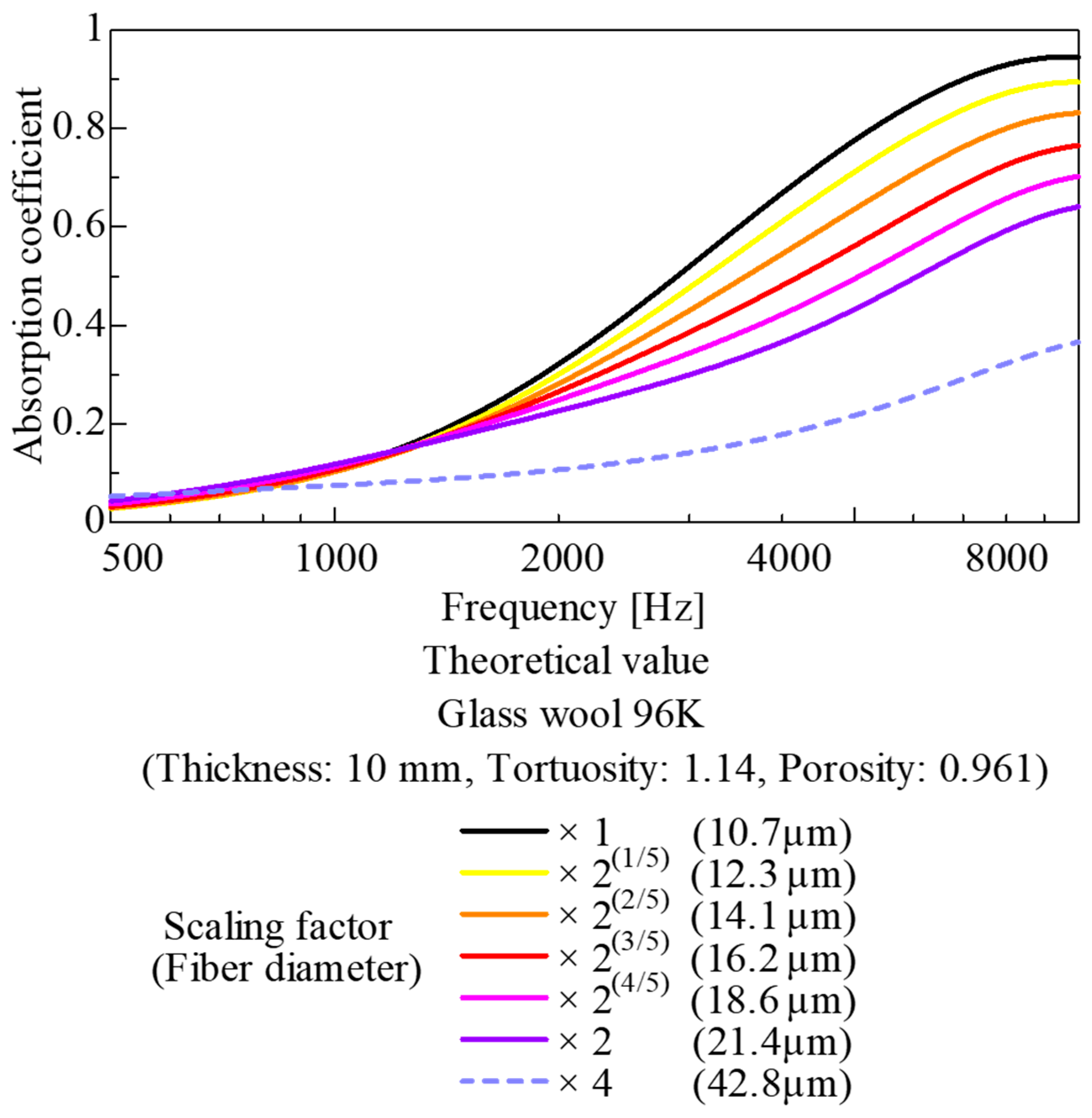
Now, consider the same CT image as above but with a voxel size of 6 μm and a circular region of 3000 pixels corresponding to a diameter of 18 mm and perform the same calculations as in the previous section. This case is equivalent to enlarging the original CT image by a factor of two under 3D similarity. In other words, this simulation represents a condition in which, compared with the original case, the fiber diameter is doubled and the surface area of the skeletal portion is halved. Furthermore, as it is three-dimensionally similar to the original case, the porosity, bulk density, and tortuosity remain unchanged.

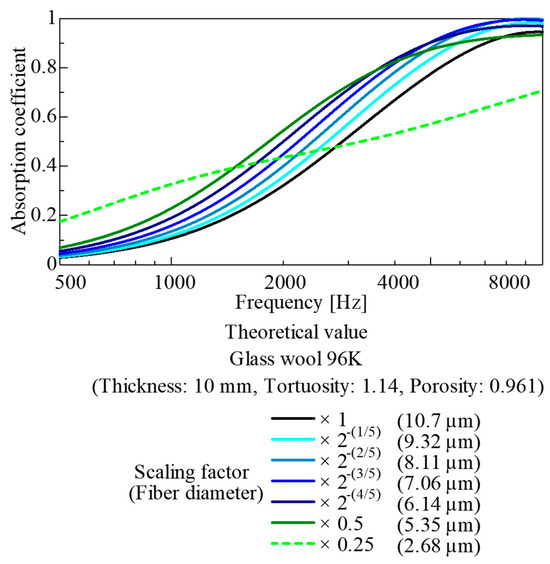
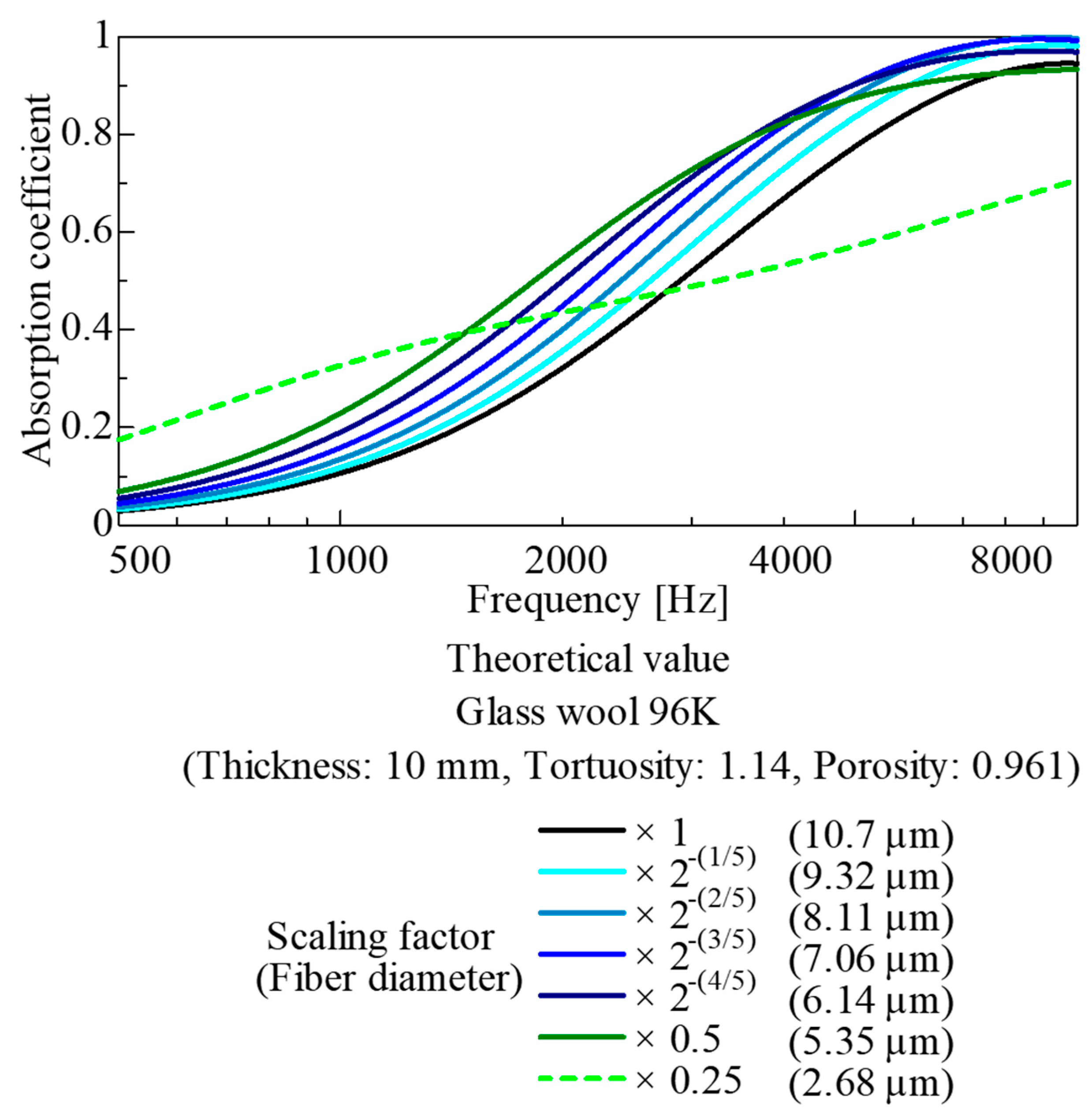
Figure 21 shows the results of a parameter study where the original CT image was gradually enlarged up to twice its size under 3D similarity. Conversely, Figure 22 shows the results of a parameter study where the original CT image was gradually scaled down to half its original size while maintaining 3D similarity.

Figure 21. Parameter study for upscaled images (based on CT images of the 96K glass wool).

Figure 22. Parameter study for downscaled images (based on CT images of the 96K glass wool).

The results in Figure 21 indicate that when the spatial dimensions and fiber diameter are gradually increased up to twice their original values under 3D similarity, the sound absorption coefficient gradually decreases at frequencies of 1 kHz and above. This is attributed to the increase in the fiber diameter and interfiber distance, causing the surface area of the fiber framework to gradually decrease. In other words, in porous materials where the interfiber distance is close to the optimum value relative to the fiber diameter—such as commercially available glass wool—enlarging the model under 3D similarity causes the interfiber distance to become excessively large and the surface area of the fiber framework to decrease. Consequently, these parameters deviate from the optimum point, leading to a deterioration in sound absorption performance. Furthermore, the simulation results for an extreme case of ×4 enlargement are shown as dashed lines.

Meanwhile, as shown in Figure 22, when the spatial dimensions and fiber diameter of the CT image were gradually reduced to a scale of 1/2 under 3D similarity, the fiber diameter and interfiber distance gradually decreased, whereas the surface area of the fiber framework gradually increased. Consequently, up to the point where the similarity ratio approached 1/2, sound absorption performance was improved compared with the original magnification. However, once the similarity ratio reached 1/2, the sound absorption coefficient conversely decreased. This decrease could be because, in porous sound-absorbing materials, sound absorption performance deteriorates when the distance between skeletal structures is too small relative to the thickness of the boundary layer on the skeletal wall surfaces. Furthermore, the simulation results for a reduction to 0.25 times the original size are shown as dashed lines as an extreme example.

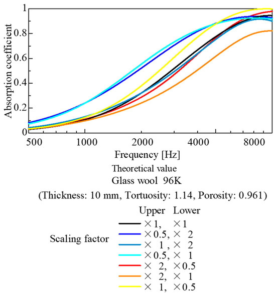
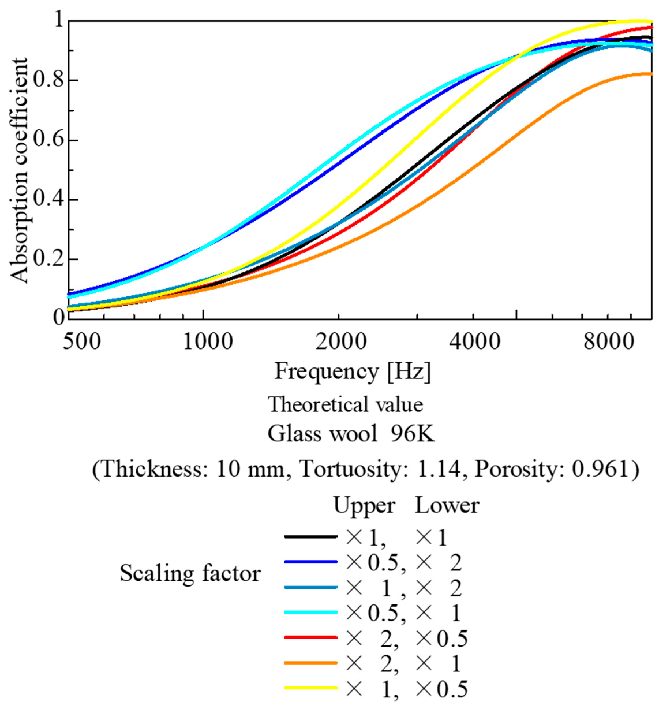
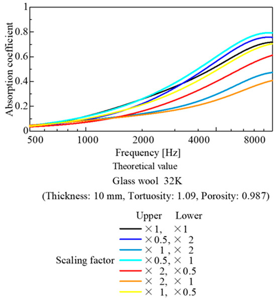
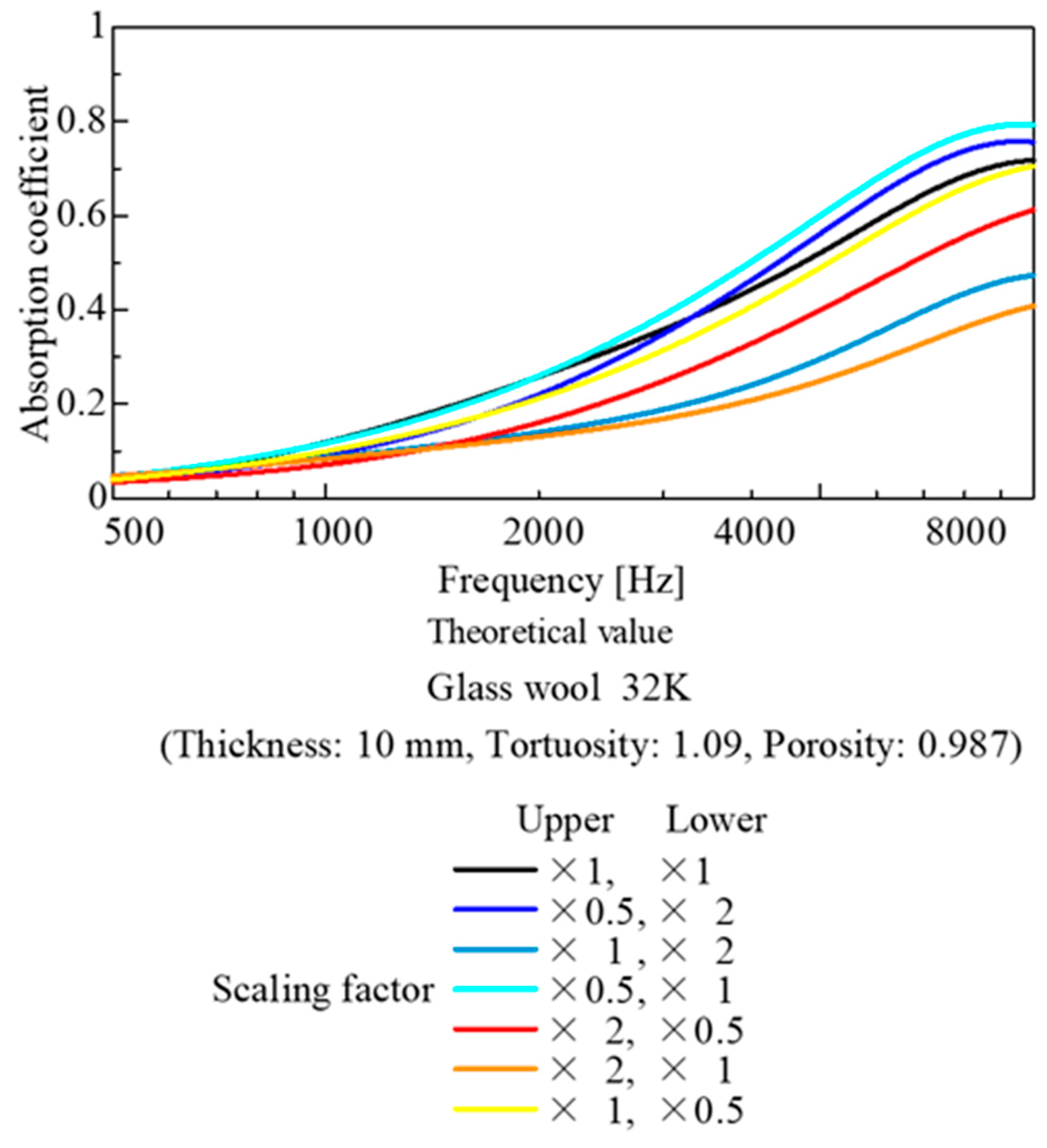
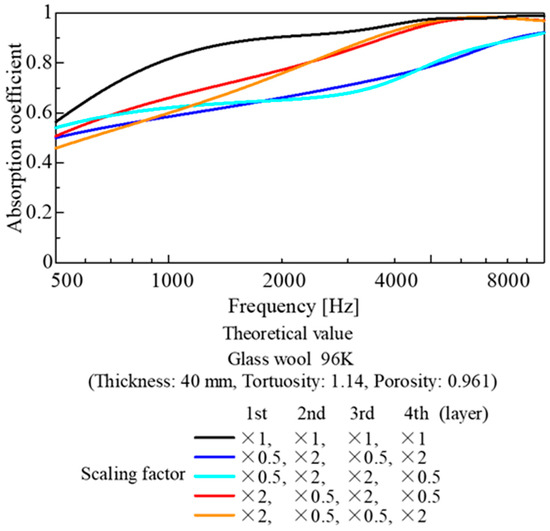
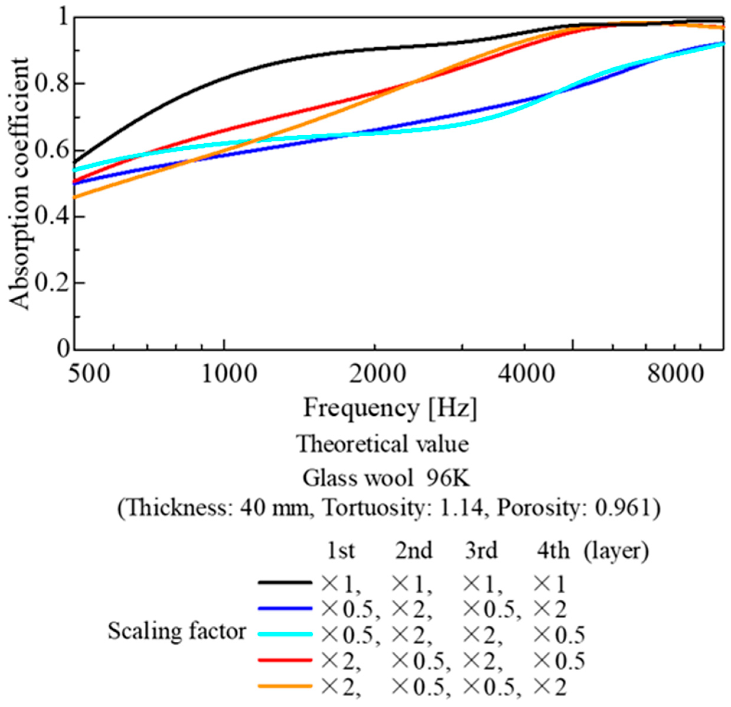
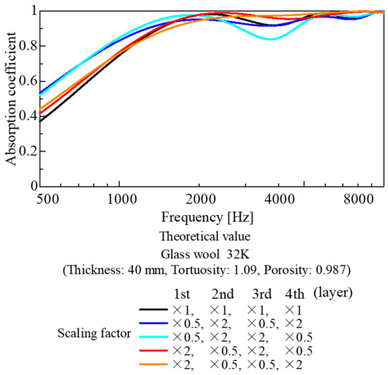
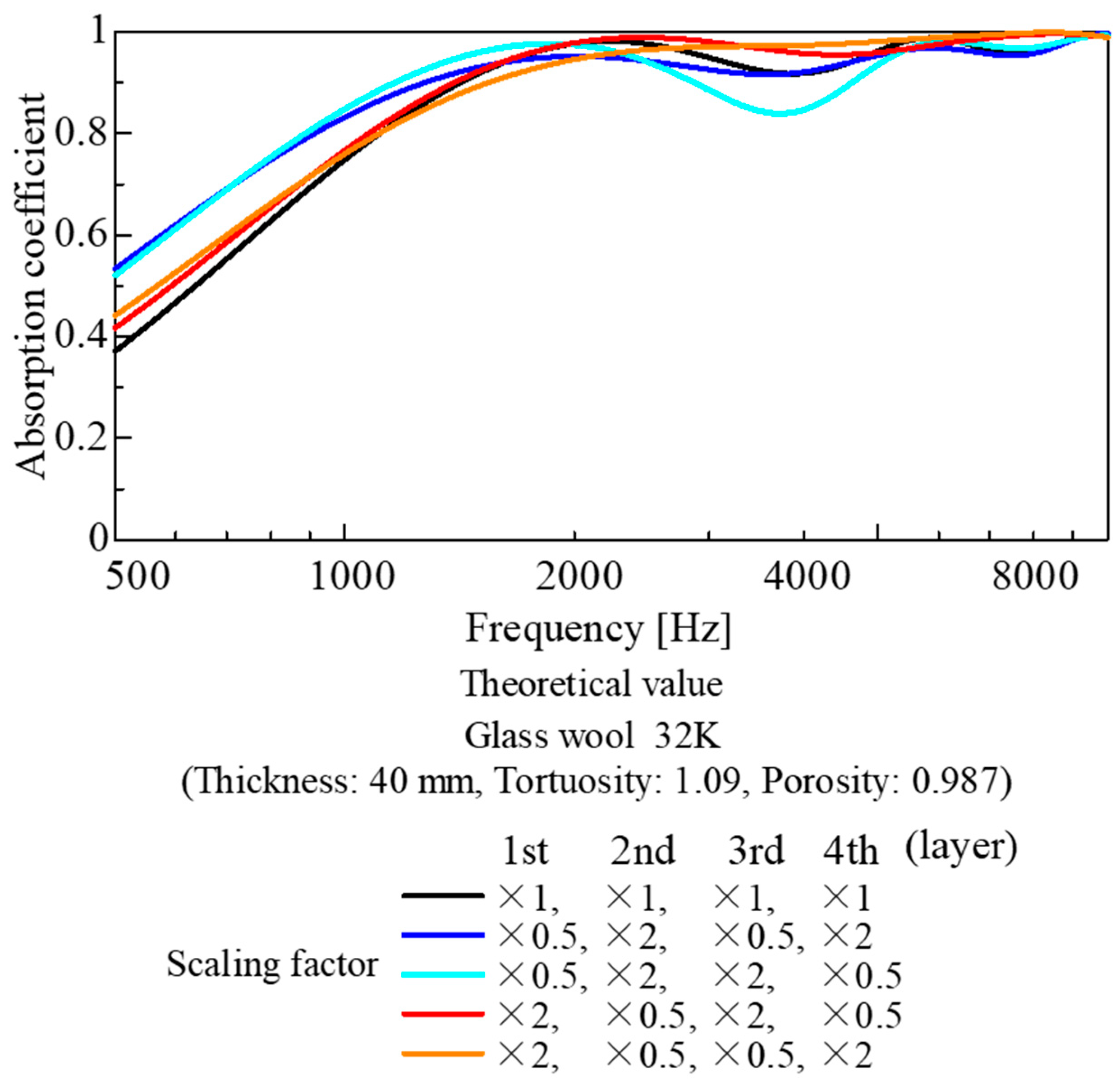
Figure 23 and Figure 24 show the results of a parametric study where image data scaled by a factor of 2 or 1/2 under 3D similarity was applied to the top 5 mm and bottom 5 mm of a 10 mm layer of glass wool, combining image data at different magnifications. Similarly, Figure 25 and Figure 26 show the calculation results obtained by dividing a 40 mm glass wool layer into four layers (10 mm each) and placing image data at different magnifications in each layer.

Figure 23. Parameter study combining upscaled and downscaled images (based on CT images of the 96K glass wool; division of 10 mm into 5 mm parts).

Figure 24. Parameter study combining upscaled and downscaled images (based on CT images of the 32K glass wool; division of 10 mm into 5 mm parts).

Figure 25. Parameter study combining upscaled and downscaled images (based on CT images of the 96K glass wool; division of the 40 mm thickness into four parts of 10 mm each).

Figure 26. Parameter study combining upscaled and downscaled images (based on CT images of the 32K glass wool; division of the 40 mm thickness into four parts of 10 mm each).

Figure 23 shows the calculation results for the 96K glass wool with a layer thickness of 10 mm. The use of a reduced-scale image in the upper layer improved the sound absorption performance. Conversely, the use of an enlarged image in the top layer reduced the sound absorption performance. This is consistent with the general finding that the material placed on the incident side significantly influences the sound absorption performance of the entire layer. Furthermore, as in Figure 21, the fact that sound absorption performance decreased in all cases when an enlarged image was used suggests that the fiber diameter and interfiber spacing of the glass wool in the original test sample were close to their optimal values.

Figure 24 shows the calculation results for the 32K glass wool, assuming a layer thickness of 10 mm (as in Figure 23). As the total surface area of the framework was small, the performance improvement when using a reduced-size image for the upper layer was smaller than in the case of the 96K glass wool shown in Figure 23. Conversely, the decline in performance when an enlarged image was used in the top layer was more pronounced than in the case shown in Figure 23. This could be attributed to the already large distance between the fibers in the 32K glass wool, resulting in a significant drop in performance when the image was enlarged.

Figure 25 shows the calculation results for the 96K glass wool, divided into four layers with a thickness of 40 mm. For example, in Figure 23, the use of a reduced image for the top 5 mm layer partially improved the sound absorption coefficient. However, in the case of the 96K glass wool, as the total area of the reduced images amounted to 23 mm, the distance between fibers became too dense compared with the optimal value considered from the boundary layer thickness. Apparently, the performance deteriorated significantly.

Figure 26 shows the calculation results for the 32K glass wool, divided into four layers with a layer thickness of 40 mm, as in Figure 25. In this case, as the distance between fibers and the surface area of the skeleton were smaller than the optimal values compared with those of 96K glass wool, the use of a reduced-scale image in the top layer slightly improved sound absorption performance in the low-frequency range. Furthermore, when an enlarged image was used in the top layer, almost no deterioration or change in performance was observed.

Figure 25 and Figure 26 show that the sound absorption curve is insensitive to changes in the image used for the upper layer. This could be because, with a sample thickness of 40 mm, the amount of the sound-absorbing material in the thickness direction is sufficiently large. Accordingly, this series of parameter studies adequately simulates the acoustic behavior of actual fiber materials.

In this study, a parameter study based on CT images was conducted. However, varying the fiber diameter and the interfiber distance independently was challenging. Nonetheless, this study also indicates potential for improvement in sound-absorbing materials relative to the current state. In the future, the use of mathematical models to simulate fiber diameter and interfiber distance (or arrangement) is expected to facilitate the model-based development of fiber-based sound-absorbing materials.

4.4. Number of Images Required for Theoretical Estimation

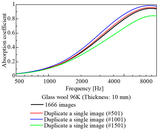
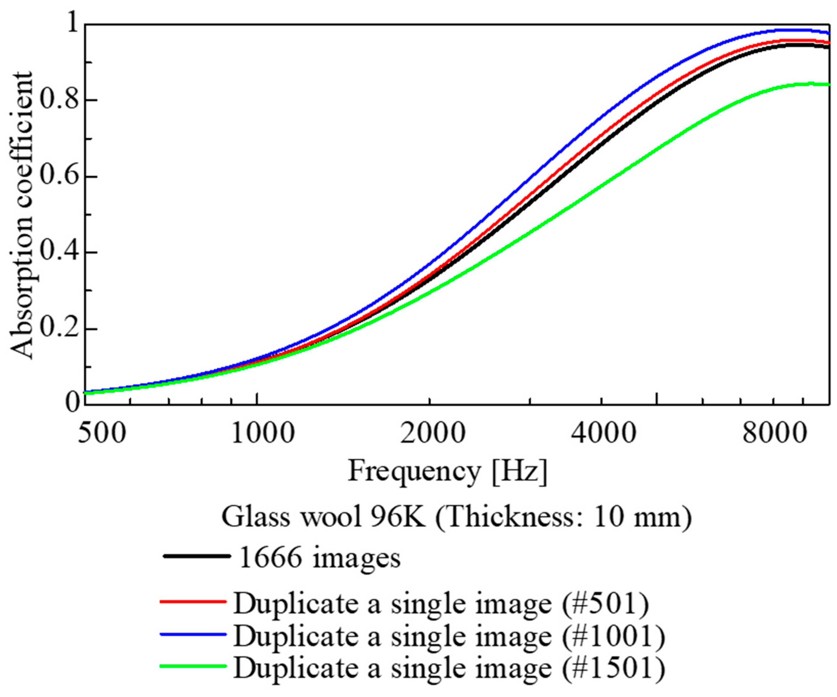
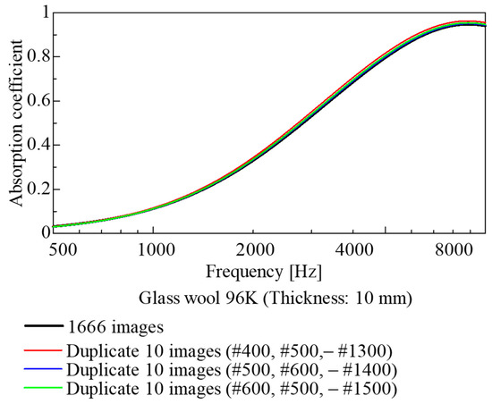
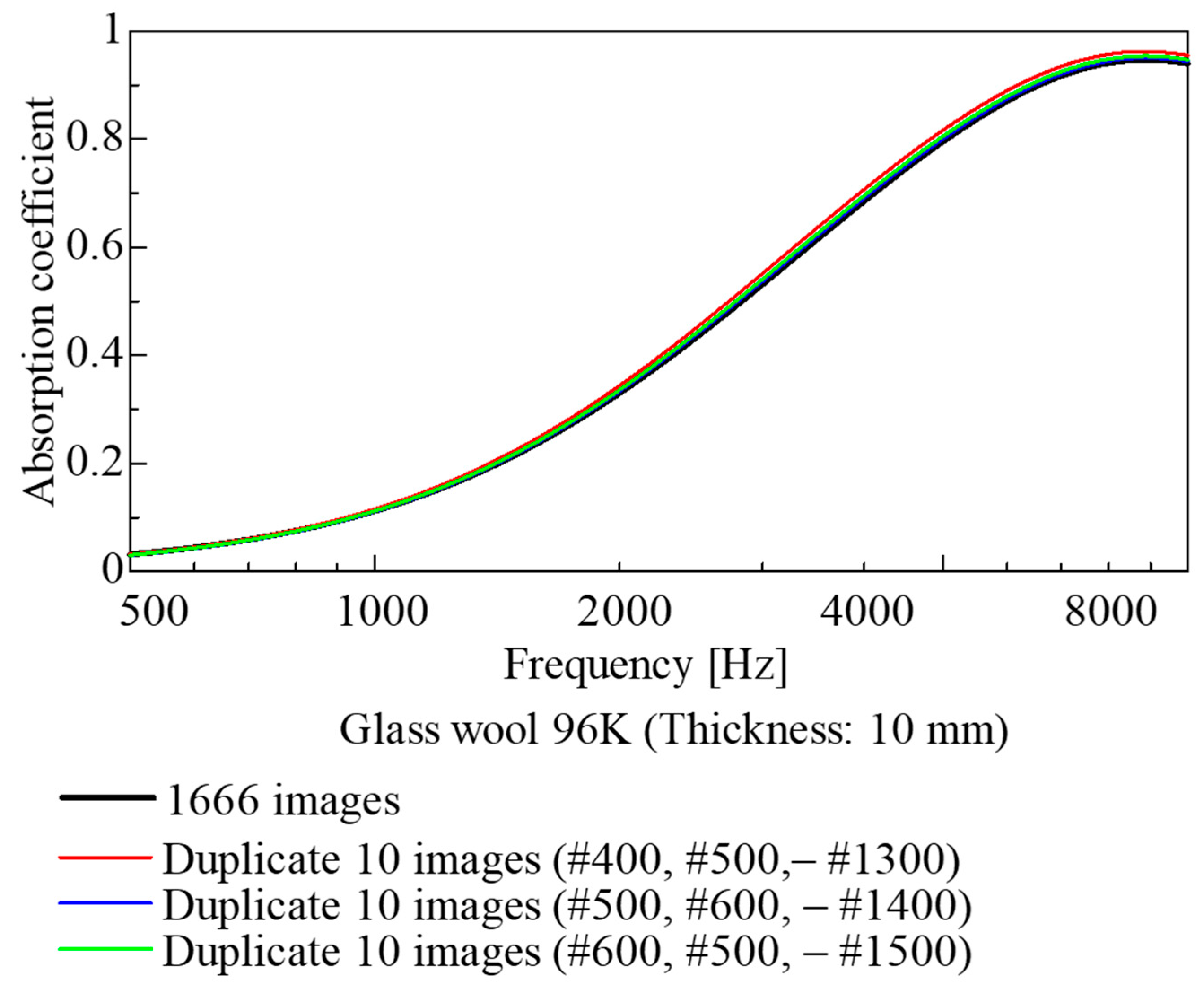
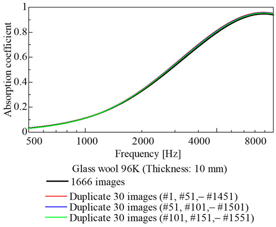
In this study, sound absorption coefficients were estimated using 1666 images captured over a 5 mm thickness range for glass wool samples. However, not all of these images are strictly necessary for estimating the sound absorption coefficient. Therefore, 1, 10, and 30 images were extracted from the set of 1666 images. Each of these sets was then duplicated to restore the original total of 1666 images, and the sound absorption coefficient was calculated using the same method as in previous analyses. The results are shown in Figure 27, Figure 28 and Figure 29.

Figure 27. Comparison of the cases using all images and duplicating a single image.

Figure 28. Comparison of the cases using all images and duplicating 10 images.

Figure 29. Comparison of the cases using all images and duplicating 30 images.

As shown in Figure 27, when a single image was duplicated 1666 times, the sound absorption coefficient varied significantly depending on the image used. Conversely, as shown in Figure 28, when 10 images were selected at regular intervals, there was almost no difference between the sound absorption curves; apparently, there was little difference even when compared with the case where all images were used. Furthermore, in Figure 29, where 30 images were selected at regular intervals, a trend similar to that above was observed, with the sound absorption coefficient almost identical to that obtained when all 1666 images were duplicated.

It follows that, for CT images of highly randomized fiber materials, employing images extracted only below a certain interval (in this case, at 0.5 mm intervals along the sample thickness) allows the estimation of the sound absorption coefficient with accuracy equivalent to that achieved when using the entire image. This leads to reductions in CT image acquisition cost and computational load.

5. Conclusions

Taking glass wool, a representative fiber-based sound-absorbing material, as the subject, this study attempted to estimate the sound absorption coefficient from cross-sectional images obtained via CT scanning. The fiber perimeter was extracted from the acquired cross-sectional images. Using this perimeter, the surface area of the fiber skeleton and the volume of the voids were calculated. The theoretical values obtained by substituting these surface areas and volumes into theoretical analyses were compared with experimental values, yielding the following conclusions.

• For each sample, the fiber surface area, accounting for fiber inclination, was calculated from the cross-sectional images obtained via CT scanning, and a transfer matrix relating sound pressure and volume velocity corresponding to each image was derived.
• Using the transfer matrices obtained above, the sound absorption coefficients for all glass wool samples were calculated for different thicknesses. Comparisons with experimental values revealed similar results.
• Through a parametric study involving the 3D image scaling, simulations of sound absorption coefficients were performed for fiber-based sound-absorbing materials with three-dimensionally analogous structures.
• Although this study can be compared with existing mathematical and finite element models in some respects, it proposes a new approach to theoretically calculate sound absorption coefficients directly from the geometric data of the actual material. This method provides a basis for model-based development in predicting sound absorption coefficients for fiber materials.

This paper focuses on glass wool, which is the most common and representative fibrous sound-absorbing material. Extending the present findings to other fibrous absorbers is left for future work.

References

- Ikpekha, O.W.; Simms, M. Effect of Acoustic Absorber Type and Size on Sound Absorption of Porous Materials in a Full-Scale Reverberation Chamber. Acoustics 2025, 7, 3. [Google Scholar] [CrossRef] [Scilit]
- Lee, J.W.; Park, S.W. Effect of Fiber Cross Section Shape on the Sound Absorption and the Sound Insulation. Fibers Polym. 2021, 22, 2937–2945. [Google Scholar] [CrossRef] [Scilit]
- Parikh, D.V.; Chen, Y.; Sun, L. Reducing Automotive Interior Noise with Natural FiberNonwoven Floor Covering Systems. Text. Res. J. 2006, 76, 813–820. [Google Scholar] [CrossRef] [Scilit]
- Shoshani, Y.; Yakubov, Y. A Model for Calculating the Noise Absorption Capacity of Nonwoven Fiber Webs. Text. Res. J. 1999, 69, 519–526. [Google Scholar] [CrossRef] [Scilit]
- Geyer, T.F.; Sarradj, E. Self Noise Reduction and Aerodynamics of Airfoils with Porous Trailing Edges. Acoustics 2019, 1, 393–409. [Google Scholar] [CrossRef] [Scilit]
- Rayleigh, J.W.S. The Theory of Sound; Dover: New York, NY, USA, 1945; Volume II. [Google Scholar]
- Delany, M.E.; Bazley, E.N. Acoustical properties of fibrous absorbent materials. Appl. Acoust. 1970, 3, 105–116. [Google Scholar] [CrossRef] [Scilit]
- Allard, J.F.; Champoux, Y. New empirical equations for sound propagation in rigid frame fibrous materials. J. Acoust. Soc. Am. 1992, 91, 3346–3353. [Google Scholar] [CrossRef] [Scilit]
- Miki, Y. Acoustical properties of porous materials—Modifications of Delany-Bazley models. J. Acoust. Soc. Jpn. 1990, 11, 19–24. [Google Scholar] [CrossRef] [Scilit]
- Komatsu, T. Improvement of the Delany-Bazley and Miki models for fibrous sound-absorbing materials. Acoust. Sci. Technol. 2008, 29, 121–129. [Google Scholar] [CrossRef] [Scilit]
- Sakamoto, S.; Hasegawa, T.; Ikeda, K. Estimation of Sound Transmission Loss in Nanofiber Nonwoven Fabrics: Comparison of Conventional Models and the Simplified Limp Frame Model. Nanomaterials 2023, 13, 2947. [Google Scholar] [CrossRef] [Scilit] [PubMed]
- Ning, J.; Li, Y. Dynamic flow resistivity and sound absorption of compressed fibrous porous materials: Experimental and theoretical. Phys. Fluids 2020, 32, 127103. [Google Scholar] [CrossRef] [Scilit]
- ISO 10534-2:2023; Acoustics—Determination of Sound Properties in Impedance Tubes—Part 2: Two-Microphone Technique for Normal Sound Absorption Coefficient and Normal Surface Impedance. International Organization Standardization: Geneva, Switzerland, 2023.
- Allard, J.F.; Castagnede, B.; Henry, M.; Lauriks, W. Evaluation of tortuosity in acoustic porous materials saturated by air. Rev. Sci. Instrum. 1994, 65, 754–755. [Google Scholar] [CrossRef] [Scilit]
- Du Plessis, J.P.; Masliyah, J.H. Flow through isotropic granular porous media. Transp. Porous Media 1991, 6, 207–221. [Google Scholar] [CrossRef] [Scilit]
- Du Plessis, J.P.; Masliyah, J.H. Mathematical modelling of flow through consolidated isotropic porous media. Transp. Porous Media 1988, 3, 145–161. [Google Scholar] [CrossRef] [Scilit]
- Bradley, D.; Roth, G. Adaptive thresholding using the integral image. J. Graph. Tools 2007, 12, 13–21. [Google Scholar] [CrossRef] [Scilit]
- Canny, J. A Computational Approach to Edge Detection. IEEE Trans. Pattern Anal. Mach. Intell. 1986, 8, 679–698. [Google Scholar] [CrossRef] [Scilit]
- Sakamoto, S.; Suzuki, K.; Toda, K.; Seino, S. Estimation of the Acoustic Properties of the Random Packing Structures of Granular Materials: Estimation of the Sound Absorption Coefficient Based on Micro-CT Scan Data. Materials 2023, 16, 337. [Google Scholar] [CrossRef] [Scilit] [PubMed]
- Sakamoto, S.; Seino, S.; Hoshiyama, K.; Kojima, Y. Estimation and experiment of acoustic properties of rice straw (estimation of sound absorption coefficient using CT images). Noise Control Eng. J. 2025, 73, 214–225. [Google Scholar] [CrossRef] [Scilit]
- Sakamoto, S.; Hoshiyama, K.; Kojima, Y.; Saito, K.; Roslan, Z.S.B. Theoretical estimation of wheat straw sound absorption coefficient using computed tomography images. Appl. Sci. 2025, 15, 8803. [Google Scholar] [CrossRef] [Scilit]
- Sakamoto, S.; Satoh, T.; Tanabe, K.; Maruyama, K.; Himori, Y. Theoretical Analysis and Experiments on the Sound Absorption Properties of Foam Sound Absorbers with Thin Membranes Naturally Present in Foams Using Nano-Computed Tomography Scan Images. Appl. Sci. 2025, 15, 11079. [Google Scholar] [CrossRef] [Scilit]
- Ishikawa, T.; Ishii, Y.; Nakasone, K.; Ohkoshi, Y.; Kim, K.H. Structure analysis of needle-punched nonwoven fabrics by X-ray computed tomography. Text. Res. J. 2017, 89, 20–31. [Google Scholar] [CrossRef] [Scilit]
- Kato, M.; Takahashi, M.; Kawasaki, S.; Mukunoki, T.; Kaneko, K. Evaluation of Porosity and Its Variation in Porous Materials Using Microfocus X-ray Computed Tomography Considering the Partial Volume Effect. Mater. Trans. 2013, 54, 1678–1685. [Google Scholar] [CrossRef] [Scilit]
- Tijdeman, H. On the propagation of sound waves in cylindrical tubes. J. Sound Vib. 1975, 39, 1–33. [Google Scholar] [CrossRef] [Scilit]
- Stinson, M.R. The propagation of plane sound waves in narrow and wide circular tubes, and generalization to uniform tubes of arbitrary cross-sectional shape. J. Acoust. Soc. Am. 1991, 89, 550–558. [Google Scholar] [CrossRef] [Scilit]
- Stinson, M.R.; Champou, Y. Propagation of sound and the assignment of shape factors in model porous materials having simple pore geometrics. J. Acoust. Soc. Am. 1992, 91, 685–695. [Google Scholar] [CrossRef] [Scilit]
- Beltman, W.M.; van der Hoogt, P.J.M.; Spiering, R.M.E.J.; Tijdeman, H. Implementation and experimental validation of a new viscothermal acoustic finite element for acousto-elastic problems. J. Sound Vib. 1998, 216, 159–185. [Google Scholar] [CrossRef] [Scilit]
- Allard, J.F.; Daigle, G. Propagation of sound in Porous Media: Modeling Sound Absorbing Materials. J. Acoust. Soc. Am. 1994, 95, 2785. [Google Scholar] [CrossRef] [Scilit]
Disclaimer/Publisher’s Note: The statements, opinions and data contained in all publications are solely those of the individual author(s) and contributor(s) and not of MDPI and/or the editor(s). MDPI and/or the editor(s) disclaim responsibility for any injury to people or property resulting from any ideas, methods, instructions or products referred to in the content. |
© 2026 by the authors. Licensee MDPI, Basel, Switzerland. This article is an open access article distributed under the terms and conditions of the Creative Commons Attribution (CC BY) license.