


Abstract
In physical chemistry textbooks, it is explained that thermodynamic processes in isolated systems (with constant internal energy) evolve until the total entropy reaches a maximum value; irreversible processes, or those in closed systems (at a constant entropy value of the system), evolve until the total internal energy reaches a minimum value; and in quasi-static processes, the maximum work is obtained under the given conditions. However, if the maximum useful work is not obtained from the system, the thermodynamic process is usually described using the Clausius inequality. Assuming that the internal energy and entropy are first-order homogeneous functions (according to Euler’s relation and additivity over system elements) and that they are state functions based on the principle of local equilibrium, the principle of maximum entropy and minimum internal energy can be applied not only to entire isolated or closed systems but to any volume element of the system. From this follows a unique discussion of the transition of a closed system (with a quasi-static isentropic process) to an isolated (irreversible) system, along with the thermodynamic process that occurs when the system remains closed and does not achieve the maximum useful work, some of which is dissipated.
1. Introduction
When an isolated or composite system (containing subsystems, i.e., compartments) undergoes a spontaneous, irreversible thermodynamic process, the differential change in its total entropy (dST > 0) is greater than zero. During this process, the differential changes in Gibbs free energy (dG) and Helmholtz free energy (dF) are equal to the negative product of the thermodynamic temperature (T) and the differential change in total entropy (dST), while the total internal energy (UT) of the isolated composite system remains unchanged: and (where p is pressure and V is volume; constancy refers both to the primary system—where the chemical reaction takes place—and to the corresponding reservoir of the composite system) [1,2,3].
In a quasi-static isentropic (reversible) thermodynamic process in a closed composite system [4,5,6], dG and dF equal the differential change in the total internal energy (dUT < 0), while the total entropy is constant: and [7,8,9].
For a system to be in equilibrium, whether it is closed or isolated, the values of dG and dF should be equal to zero.
According to the definition of Williamson and Morikawa [10], the maximum useful work of a thermodynamic process (primarily referring to the chemical reaction in galvanic cells and fuel cells) implies a part of the internal energy change of a given thermodynamic process that can be used freely for any purpose (if the process is isentropic, then it may be necessary that part of the change in internal energy be spent to compensate for the change in entropy). The maximum useful work is obtained during reversible thermodynamic processes. Of course, the maximum useful work depends on the conditions under which the observed thermodynamic process occurs. So, for example, at a constant temperature, the maximum useful work is equal to the maximum work, i.e., a change in the Helmholtz free energy if there is no volume–pressure work (if the volume is constant). Meanwhile, if the temperature and pressure are constant, then the maximum useful work is equal to the change in Gibbs free energy, i.e., maximum non-expansion work [4,7,10].
It is natural to wonder what happens when the total internal energy and the total entropy of a composite system change simultaneously (). This is a topic of significance in thermodynamics and chemical engineering. The goal was to achieve a quasi-static isentropic (reversible) thermodynamic process in the primary system during an idealized galvanic or fuel cell chemical reaction. However, some part of the maximum useful work is lost if the chemical reaction in the composite system does not correspond to a hypothetical isentropic process or if the chemical reaction in the composite system is isentropic but is coupled with a secondary spontaneous irreversible processes, such as friction during piston movement in a cylinder or resistance when current flows through a conductor [10]. As a result, the composite system is still closed; however, some of the internal energy changes in the quasi-static isentropic (reversible) process remain as thermal energy due to the secondary irreversible process [11,12,13,14,15,16].
The goal of this study is to describe the thermodynamic process from which the useful work is obtained. This work, in terms of absolute value, is smaller than the absolute value of the maximum useful work obtained from the hypothetical isentropic (reversible) thermodynamic process. We achieve this by applying the principles of minimum total internal energy and maximum total entropy to the specific volume of the observed system where a thermodynamic process (chemical reaction) occurs. In this context, the system’s volume elements, a key aspect of the principle of local equilibrium, play a crucial role. In a new approach, the equation −TdST = dUT is not used to transform the entire composite system from a closed to an isolated one. Until now, only the equation −TdST = dUT has been applied in such transformations, while it is applied in this study for the case that the system is further closed (i.e., work is obtained from the composite system), and −TdS = dU is applied only for certain elements of the system’s volume (where dS and dU refer to the observed volume element of the system). In this way, it is possible to explore the possibility of changing the regime of thermodynamic processes:
- The quasi-static isentropic (reversible) process completely turns into an irreversible thermodynamic process, i.e., a closed system (from which the maximum useful work is obtained under given conditions) turns into an isolated system (where zero useful work is obtained).
- When a closed system partially turns into an isolated system, some elements of the volume of the system formally become completely isolated (reversible processes in these elements of the volume completely turn into irreversible processes). In contrast, some elements of the volume remain closed systems with reversible processes—a lower absolute value of useful work is obtained from the whole system compared to when only quasi-static isentropic processes are carried out within it.
The present discussion of analog processes hold significance for the pedagogical introduction of concepts such as the maximization of useful work and its dissipation.
2. Materials and Methods
In this study, we apply the principle that internal energy and entropy are state functions and that they are homogeneous functions of the first order of extensive state quantities (Appendix A and Appendix B).
3. Results and Discussion
3.1. Two Extremes and De Donder’s Equation
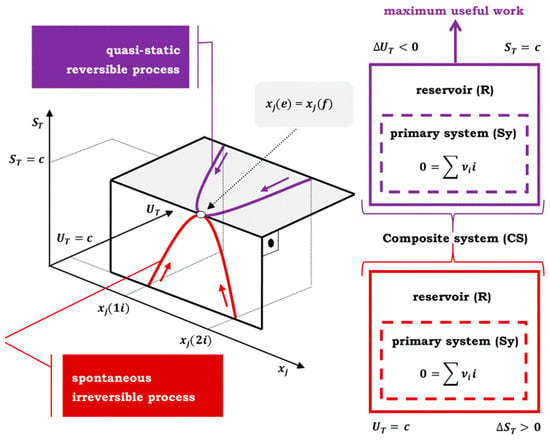
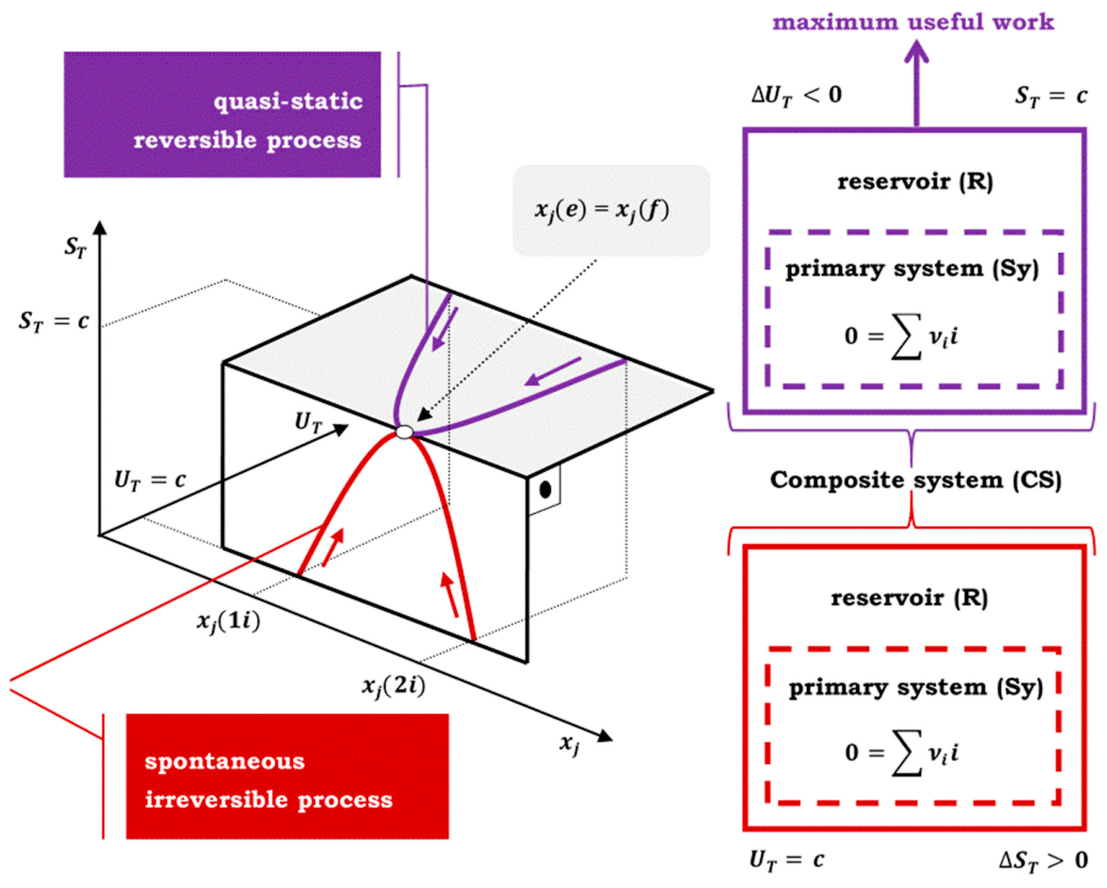
Consider a system whose state changes from an initial value of either xj(1i) or xj(2i) during a thermodynamic process. As the system reaches equilibrium in this process xj(e), it will arrive at a final state, denoted as xj(f), regardless of the type of system involved. In an isolated system, the total internal energy remains constant while the total entropy increases until equilibrium is achieved. Conversely, in an isentropic closed system, the total internal energy decreases until the system also reaches its final equilibrium state (Figure 1).
Figure 1.
The total entropy (ST) of an isolated system (the total internal energy is constant (c)) increases to the equilibrium state and the total internal energy (UT) in a closed system decreases until the equilibrium state is established.
Generally, let us consider a closed composite system (CS, Figure 1) that becomes isolated. In this scenario, the differential change in the total internal energy (dUT) due to the thermodynamic process remains in the system as energy that is distributed over different molecular degrees of freedom, increasing the total entropy for the differential value (dST)—i.e., this is a spontaneous, irreversible process [7,9]:
Equation (1) is actually a more general form of De Donder’s Equation (2) [1,17], which describes the production of entropy in an isolated system during a chemical reaction—entropy produced by the irreversible processes ():
where and represent the chemical potential and stoichiometric coefficient of the i-th compound in the observed reaction , respectively. In Equation (2), A is the De Donder affinity of the reaction and dξ corresponds to the infinitesimal extent of the chemical reaction [18]. As the chemical potential is the partial molar Gibbs free energy, then it can be expressed with the partial molar enthalpy () and entropy ():
If the reaction takes place at constant temperature and pressure, then, based on the partial molar properties [19], it follows that
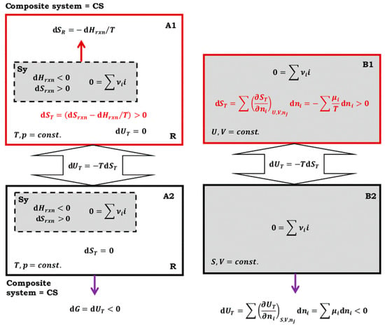
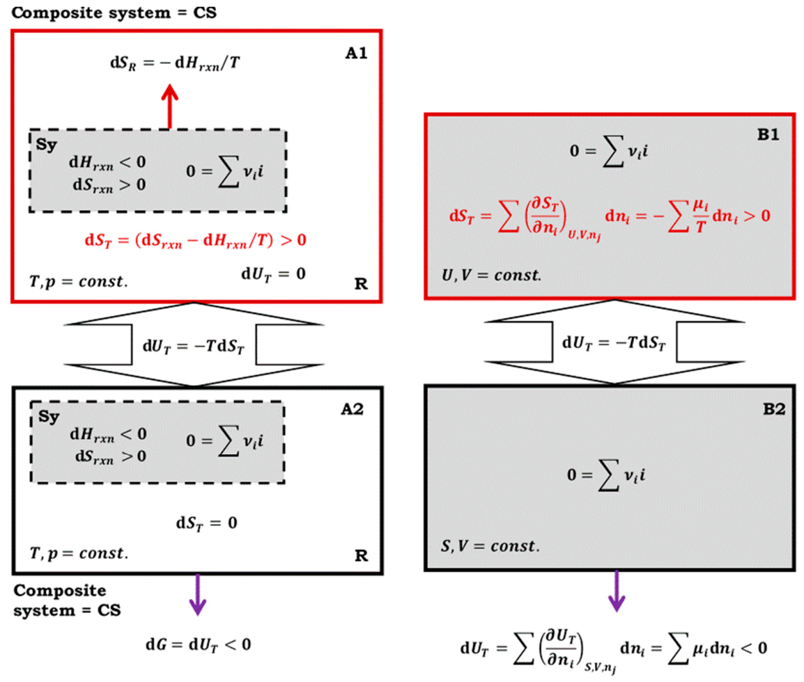
According to Callen [7], the equality holds, from which Equation (5) follows. rxn means that the thermodynamic functions change during the progress of the chemical reaction. In an isolated composite system, () represents the differential change in entropy in the pressure–temperature reservoir (), while corresponds to the differential change in entropy in the primary system in which the chemical reaction takes place, which means that De Donder’s differential change in entropy corresponds to the differential change in total entropy (dST) of the isolated composite system (Figure 2).
Figure 2.
Meaning of De Donder’s equation: (A1), isolated composite system (Sy = primary system and R = T, p reservoir); (A2), closed composite system; (B1), isolated system with constant volume and without a reservoir of intensive thermodynamic parameter; (B2), closed system with constant volume and without a reservoir.
Equality from De Donder’s equation can also be proven under constant V conditions when the system lacks a reservoir of an intensive state parameter, i.e., the system is a simple system rather than a composite. The chemical potential is defined not only as the partial molar Gibbs energy but also as the partial derivative of the internal energy with respect to the amount of the i-th component, while keeping the volume and entropy constant, as well as accounting for the amounts of other components: . Therefore, the right-hand side of the equation in expression (3) represents the differential change in the total internal energy of a simple system at constant entropy and volume (Figure 2):
3.2. Loss of Working Capacity of the System in Which the Chemical Reaction Takes Place
Winterbone defines the irreversibility parameter (I) as the amount of energy associated with the useful work lost in a thermodynamic process. It describes the difference between the maximum possible useful work obtainable in a purely quasi-static isentropic (reversible) process and the actual useful work carried out when irreversible thermodynamic processes are also involved. In this context, the absolute value of the useful work is considered in the difference, ensuring that Winterbone’s measure of irreversibility is always a positive quantity [20,21].
Let us consider a system divided into two parts (Figure 3). One part always undergoes a quasi-static isentropic (reversible) process, during which the intensive state variables remain constant throughout the entire compartment. Naturally, intensive state variables change during a quasi-static thermodynamic process (intensive variables that are not under constraint). However, at each process evolution point, they have identical values in the entire compartment. Conversely, the other part of the system can undergo both quasi-static isentropic (reversible) processes and irreversible processes. When irreversible processes occur, the intensive state variables will differ at various locations within the compartment. Since internal energy and entropy are additive across the elements of a system—where these elements can be either tangible compartments of the composite system (CS) or theoretical constructs—at a certain point in the quasi-static thermodynamic process, we can express the total internal energy of the composite system as the sum of the following (Appendix A):
Figure 3.
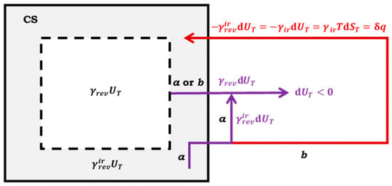
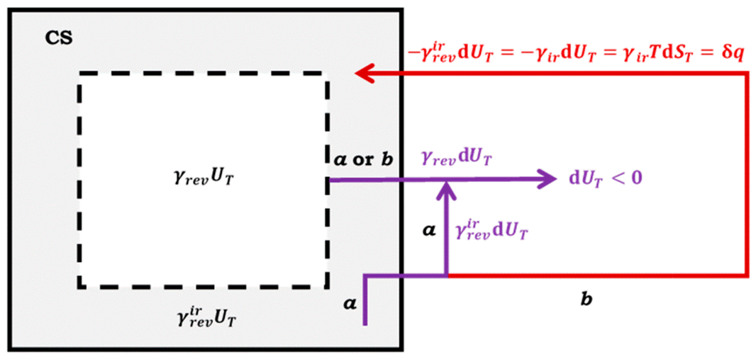
Composite system (CS) with two real or imaginary compartments; in the case of a, a quasi-static reversible process takes place, while in b, an irreversible process takes place in addition to a quasi-static reversible thermodynamic process.
In Equation (7), represents the fraction of internal energy (or volume) of the composite (real or imaginary) system, where a quasi-static isentropic (reversible) process always takes place (Appendix B), while in the part of the CS irreversible thermodynamic processes, in addition to the quasi-static process, can also take place. Let it be assumed that the fractions and remain constant during the thermodynamic process ( + = 1). The differential change in the total internal energy of the composite system due to the infinitesimal progress of a quasi-static reversible thermodynamic process (without an irreversible process in the part of CS—Figure 3, path a) is as follows (Appendix A):
Let the observed reversible thermodynamic process have a change in entropy of zero, i.e., if a chemical reaction is observed, then it is (Appendix C). Then for the part of the composite system (CS) where the quasi-static reversible process always occurs, the following relation is valid:
Suppose that the quasi-static reversible process takes place in the part of the imaginary composite system where both the quasi-static reversible and the irreversible processes can occur. In that case, it is as shown in Figure 3.
Presume that a spontaneous irreversible process occurs in the part of the CS. In that case, formally, part of the differential change in the total internal energy () of the hypothetical quasi-static reversible process returns to the system as differential heat ( refers to a quasi-static thermodynamic process with , i.e., formally, a quasi-static reversible process occurred first, followed by a spontaneous irreversible process; Figure 3, path b):
Since the system is further closed at the part where the quasi-static reversible process exclusively takes place (), the differential change in internal energy (, which leaves the CS) does not contribute to the differential entropy change (9) in the CS (Figure 3). While a spontaneous irreversible process now takes place, in addition to a quasi-static reversible thermodynamic process (which first happened), in part of the CS (), some of the change in the total internal energy of a quasi-static reversible thermodynamic process () remains in the imaginary part of the system generating entropy (the portion of internal energy that is dissipated: ). In line with this, Equation (1) demonstrates the case of a transition from a quasi-static reversible regime to a system where, in addition to a quasi-static reversible process, there is also a spontaneous irreversible process (the system is closed; Figure 3, path b):
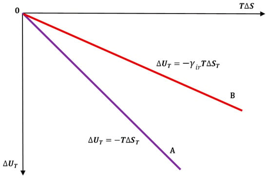
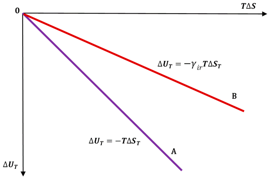
In Equation (13), refers to the differential change in the total internal energy in CS if a quasi-statically reversible thermodynamic process takes place in each real or imaginary compartment (formally, which occurred before the irreversible process). The actual differential change in the total internal energy of the CS is and the composite system remains in the form of useful differential work (Figure 3, path b). Since both internal energy and entropy are state functions, Equation (13) can be expressed in its integral form as , which represents a functional dependence where each value of corresponds to a specific value of , indicating the portion of internal energy change that is dissipated within the system. In a closed system undergoing a hypothetical reversible thermodynamic process (with ), the system remains closed. However, during an irreversible process, a portion of is dissipated within the system—in the case of a system transitioning from a closed type to an isolated one, holds (Figure 4). It follows from Equation (13) that
and taking into account Equation (12),
Figure 4.
A: A closed system with a reversible exothermic chemical reaction is transformed into an isolated system. B: A closed system remains closed, i.e., useful work is obtained from the system, but part of the internal energy change in a hypothetical reversible process is wasted in an irreversible process.
In the last expression (15), corresponds to the useful differential work, which would be obtained if the thermodynamic process in the composite system (CS) were entirely quasi-statically reversible (Figure 3, path a):
represents the real useful differential work that is obtained if there is also a parallel irreversible process (Figure 3, path b):
Therefore, the difference on the left side of Equation (15) is the differential part of the change in the total internal energy that is wasted in the form of thermal energy during an irreversible process (wasted work potential—dissipated energy) and leads to the generation of entropy:
In Equation (18), and since these are differential changes in the total internal energy of the composite system that leaves the system in the form of useful work. However, for infinitesimal (differential) dissipated energy, the differential irreversibility parameter (δI) is . Namely, Winterbone’s irreversibility parameter is part of the change in the total internal energy of the composite system during some hypothetical reversible process, which remains in the given composite system [20], i.e., formally, it returns to the composite system during an irreversible process as (Figure 3, path b). If, at every moment of the thermodynamic process in the composite system, there is an internal equilibrium (hypothetical limit case), then a quasi-static reversible process takes place in the entire composite system. Hence, the value of Winterbone’s irreversibility parameter is equal to zero:
It can be shown that Equation (19) results from the Clausius inequality [22], namely, dividing by T yields the expression
Bearing in mind that originates from an irreversible process, which means that it represents Prigogine’s entropy change due to “uncompensated transformation” [1], the entropy produced by the irreversible processes () is
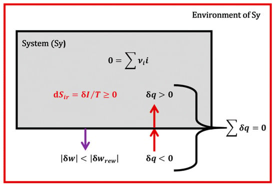
Let the system (Sy)—or the imaginary composite system CS (Figure 3)—be closed to the environment (Figure 5) and let heat transfer from the environment to the system under isothermal conditions ; then, inequality (22) is:
where represents the differential change in entropy in the system. By rearranging the inequality (23), the usual form of the Clausius inequality is obtained:
Figure 5.
In a closed system, the entropy of an irreversible thermodynamic process—an uncompensated change in entropy—is generated if there is isothermal heat exchange between the environment of the system. Then, the change in entropy (due to heat transfer) in the environment is compensated with the entropy exchange in the system.
Equation (18) is a general expression and is valid regardless of the presence of a reservoir of intensive quantities and unchanged extensive quantities of the system (for example, a constant volume (Appendix C)), i.e., Equation (16) can be applied to any thermodynamic potential [7,16,23,24]. The following equations calculate the differential change in the thermodynamic potential of a quasi-statically reversible thermodynamic process:
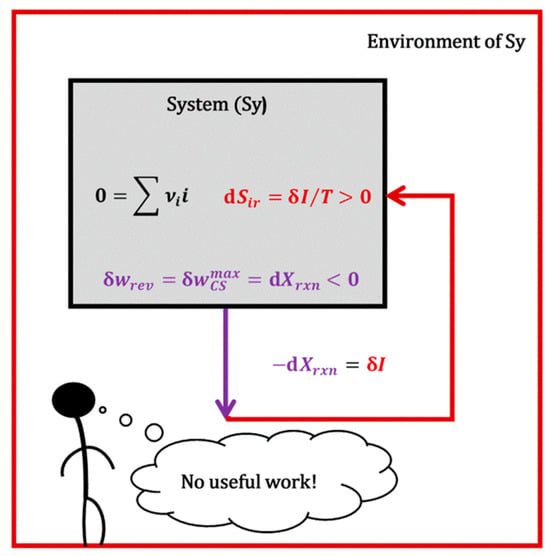
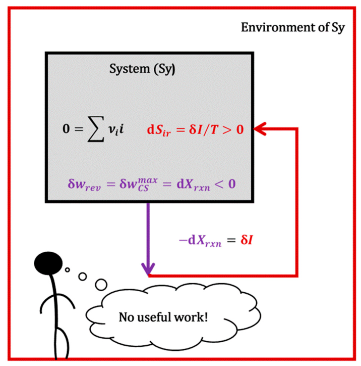
If in Equation (26) the useful work () is zero, i.e., no useful work is obtained from the system where the chemical reaction takes place, whereby the change in (maximum useful work) is completely lost in an irreversible process (Figure 6), then the equation is
Figure 6.
No useful work is obtained from the system, and the maximum useful work formally turns into heat, which generates the entropy of the irreversible process.
If the thermodynamic process is in equilibrium, then ; therefore, the following equality follows from Equation (26):
Considering De Donder’s Equations (2) and (4), expression (27) for p,T = const. can be expressed as follows (where ):
The differential entropy change () in an irreversible thermodynamic process can be represented as the product of the thermodynamic force ()— the difference between the intensive state variable of the system in the entropy representation between neighboring parts of the system—and an extensive physical quantity (corresponding to the intensive quantity) that is transported during the dt time interval () [1,23]:
Alternatively, in a system in which intensive state variables are continuously changing (taking into account the flux of the extensive variable (, where M is the surface normal to the flux direction), the entropy generation per unit of time and volume () can be calculated as follows [25]:
where g represents the Gibbs free energy per unit volume, while is the gradient of the intensive state variable in the entropy representation. Equation (31) is valid for the entire system (during an infinitesimal time interval dt); in addition, it can also be applied to some imaginary volume element of the system in which a generalized thermodynamic force occurs, . When the primary system experience fluctuations in chemical reaction velocity, the system’s behavior becomes more complex. In some parts of the volume, the reaction runs faster than the hypothetical infinitely slow chemical reaction, causing a deviation from the state with uniform velocities for each volume element. This dynamic behavior leads to non-uniform concentrations of reactive components across the volume elements of the primary system. In addition to the thermodynamic force of the chemical reaction A/T (i.e., , in Equation (30)), the dynamic system also gives rise to the thermodynamic force of diffusion of reactive components:
( differential amount of the k-th reactive component that diffuses in the dt time interval and = chemical potential gradient). The appearance of the thermodynamic force of diffusion can reduce the chemical potential of a reactive component in some volume element of the primary system. This, in turn, significantly influences the De Donder affinity (A) of the chemical reaction. The result is the absence of in some volume elements of the primary system, leading to the absence of useful non-expansion work. However, the most significant impact is entropy generation due to the irreversible diffusion process (Equation (32)), a crucial aspect of the system’s behavior.
The hypothesis of local equilibrium allows us to assume thermodynamic equilibrium in different parts of a system, even when the overall system is out of equilibrium (Appendix A). This concept enables the development of a theory that describes the behavior of macroscopic systems under nonequilibrium conditions, known as the thermodynamics of irreversible processes [1]. However, this theory has its limitations. Firstly, it is valid only as long as the hypothesis of local equilibrium holds. Secondly, the thermodynamics of irreversible processes is fundamentally a linear theory; thus, it applies only to situations where the thermodynamic laws can be expressed as linear functions of generalized thermodynamic forces, which are the gradients of thermodynamic state variables. This condition implies that the system is relatively close to equilibrium, meaning fluctuations in the state variables are small [1,7]. As the characteristic time or length scales of the system decrease, Onsager’s proposal becomes inadequate for describing these systems. At the mesoscopic level, where fluctuations in thermodynamic variables can be significant, it is necessary to adopt a probabilistic approach to these variables. P. Mazur formally developed what is now known as mesoscopic nonequilibrium thermodynamics (MNET) [26]. Decreasing the characteristic length and time scales of a system requires introducing additional thermodynamic degrees of freedom. At the mesoscopic level, the state of the system is represented by a probability density, P(γ,t), where γ serves as an order parameter encompassing all microscopic degrees of freedom, such as positions, velocities, and orientations. By ensuring the conservation of probability in γ-space and applying the principles of linear nonequilibrium thermodynamics in this space, the Fokker-Planck equation can be derived, which describes the evolution of the system’s probability distribution. By obtaining this probability distribution, one can extract all the thermodynamic information about the system [27]. For instance, MNET can be used to study the conformational distributions of polymers, the dynamics of colloidal particles, nucleation and growth during phase transformations, transport through ion channels in cell membranes, and the operation of nanomotors, among others [27,28,29]. In the diffusion processes far from equilibrium, the hypothesis of local equilibrium can remain valid by extending the vector space to include the velocity coordinate alongside the spatial coordinates. This is because the relaxation of the velocity distribution and changes in density occur on the same timescale. Thus, the chemical potential according to MNET in one-dimensional space (x) with an additional velocity coordinate (v) is:
where m is the mass of the particles, k the Boltzmann constant, n(x,v) is the density and C(x,v) a function that takes into account spatial inhomogeneities. In molecular systems such as suspensions of rod-like particles, liquid crystals, polarized systems and field-responsive suspensions, the internal variable can be the angular coordinate (θ, takes into account the position of the molecule in relation to a vector field), so the chemical potential of the particles is:
where is the orientational potential energy and is a function for the orientational degeneracy [27].
4. Conclusions
It is shown that, for chemical reactions, De Donder’s equation fully corresponds to the equation −TdST = dUT when the composite system changes from a closed system to an isolated system. De Donder’s entropy change for an irreversible process equals the total entropy change in the system, whether it is a simple or composite system.
In this paper, the equation −TdS = dU is not applied for the transformation of a composite system from a closed to an isolated one (so far the equation −TdS = dU has only been applied in such transformations), but it is applied in the sense that the system is further closed (i.e., work is obtained from the composite system) and that the equation −TdS = dU is applied only for certain elements of the system’s volume, so not for the entire system (in some parts of the system the chemical reaction is quasi-static and isentropic, while in some parts it is irreversible, i.e., the work is obtained from some elements of the system’s volume and not from others). Applying the equation −TdS = dU or to a real or imaginary compartment of a system, i.e., to the volume elements of the system, and by applying the same equation to the entire system, the theory of maximum entropy and minimum internal energy is uniformly applied, regardless of whether it is a complete transformation of a closed system into an isolated one, or whether this transformation is of a local nature. The above is in full agreement with Prigogine’s principle of local entropy production [1]:
or, as, an equivalent expression to (35),
According to this, not only is the system’s total entropy change zero or greater, but each element of the system shows an increase in entropy in irreversible processes or a constancy of entropy in reversible processes. According to Equation (36), the system (or its elements) does not require any restriction in the sense of an open, closed, or isolated system. Therefore, it is possible that entropy is generated in some elements of the system without obtaining work, while in others the maximum useful work is obtained in a quasi-static isentropic process.
Funding
This research received no external funding.
Institutional Review Board Statement
Not applicable.
Data Availability Statement
The original contributions presented in this study are included in the article.
Conflicts of Interest
The author declares no conflicts of interest.
Abbreviations
The following abbreviations are used in this manuscript:
| differential change in total entropy | |
| differential change in total internal energy | |
| differential changes in Gibbs free energy | |
| differential changes in Helmholtz free energy | |
| chemical potential of the i-th compound | |
| stoichiometric coefficient of the i-th compound | |
| the infinitesimal extent of the chemical reaction | |
| differential entropy produced by the irreversible processes | |
| the De Donder affinity of reaction | |
| partial molar enthalpy | |
| partial molar entropy | |
| rxn | the thermodynamic functions change during the progress of the chemical reaction |
| Sy | system |
| R | reservoir |
| CS | composite system |
| I | Winterbone’s irreversibility parameter |
| fraction of internal energy (or volume) of the composite (real or imaginary) system where a quasi-static isentropic (reversible) process always takes place | |
| part of the CS; in addition to the quasi-static process (), irreversible thermodynamic processes can also take place () | |
| the useful differential work that would be obtained if the thermodynamic process in the composite system (CS) were entirely quasi-statically reversible | |
| the real useful differential work that is obtained if in the CS there is also a parallel irreversible process | |
| differential heat | |
| differential change in the thermodynamic potential of a quasi-statically reversible thermodynamic process (chemical reaction) | |
| Helmholtz thermodynamic potential at constant volume and temperature | |
| enthalpy thermodynamic potential at constant pressure and entropy | |
| Gibbs thermodynamic potential at constant pressure and temperature | |
| differential change in entropy in the system | |
| thermodynamic force | |
| flux of the k extensive variable | |
| M | surface normal to the flux direction |
| entropy generation per unit of time and volume | |
| g | Gibbs free energy per unit volume |
| u | internal energy density |
| average values of the internal energy density by volume elements |
Appendix A
Figure A1.
A: The non-equilibrium system in the initial and final state is divided into elementary volumes by which the internal energy density is constant ( and —kth volume element). The non-equilibrium real system is shown with volume elements characterized by average values of the internal energy density ( and ). B: A reversible thermodynamic process that is characterized by an equilibrium state of the system at each point of the process, including the initial and final states ( and ). C: A real non-equilibrium system (from process A) is represented so that both in the initial and in the final state, each volume element is divided into two parts—the part that corresponds to the equilibrium state ( with and ) and the part that is not subject to change (part of the volume element that does not contribute to obtaining useful work, where the greater the degree of irreversibility, the greater the fraction of this volume element). C1 and C2: Systems in which the equilibrium volume elements and volume elements in which the internal energy does not change are collected in the initial and final states.
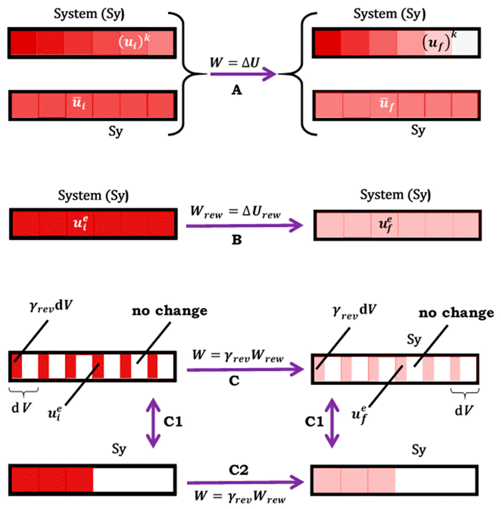
Let the system from which, during a thermodynamic process (chemical reaction with ), the useful work is obtained be divided into volume elements where the intensive state variables are approximately constant [1]; between the volume elements, the values of the intensive state variables can change. The change in the internal energy of the system as a result of the thermodynamic process is equal to the useful work (which is not the maximum useful work):
where represents the final state of internal energy, and corresponds to the initial state of internal energy. In general, each volume element of the system (in the final and initial states) is characterized by an internal energy density ( and ) that depends on the coordinates of the volume element (Figure A1):
Let the internal energy densities in Equation (A3) be expressed with the average values of the internal energy density by volume elements of the system:
If there is an equilibrium state in the system both before and after the quasi-static isentropic thermodynamic process, whereby the internal energy densities are equal in every point of space, i.e., volume, then Equation (A3) is
Let the useful work be expressed as a share of the maximum useful work, so that the coefficient is constant during the thermodynamic process (Figure A1):
From Equation (A8), we obtain the following (where ):
Equation (A6) defines the coefficient :
Appendix B
The internal energy of a system is a homogeneous function of the first order with respect to the extensive state quantities: entropy (S), volume (V), and the number of moles (n) of the components that make up the observed system. As a result, we can express the internal energy in relation to the internal energy of an element. Here, λ represents a constant—meaning it can indicate either an increase (λ > 1) or a decrease (λ < 1) in internal energy relative to that of the element.
According to the Tisza-Calen concept [7,30], imposing an appropriate constraint can halt the thermodynamic process. While the given constraint exists, the system is in equilibrium (conditional equilibrium), where expression (A11) holds. Multiplying the last expression by gives
where represents the part of the system in which a quasi-static thermodynamic process is always taking place, with the constant removal and restoration of the appropriate constraints (in hypothetical infinitesimal steps).
Appendix C
For example, consider a quasi-static isentropic thermodynamic process, which is a chemical reaction in a primary system of constant volume (V = const.) and in contact with a thermoreservoir, T = const. (composite system (CS) of the primary system and the thermoreservoir). When there is an infinitesimal change in the reaction extent, the differential change in internal energy (primary system) is , while the differential change in entropy (primary system) is . Since the observed chemical reaction is reversible, the differential change in the total entropy of the composite system is zero:
where is the differential entropy change in the thermoreservoir. The differential change in the internal energy of the thermoreservoir is
Therefore, the differential change in the total internal energy of the CS is
Equation (A15) defines the differential change in the Helmholtz free energy [7,8,9], which is equal to the (differential) maximum work that can be “extracted” from a chemical reaction. If Equations (8)–(16) refer to a composite system with a thermoreservoir, then if in the CS, in addition to a quasi-static isentropic chemical reaction, there is also an irreversible thermodynamic process taking into account Equation (A15), we have the following:
From Equation (17), we have
From Equations (A16) and (A17), it follows that
References
- Kondepudi, D.; Prigogine, I. Modern Thermodynamics, From Heat Engines to Dissipative Structures; John Wiley & Sons: Chichester, UK, 2002; pp. 125–130. [Google Scholar]
- Teixeira-Dias, J.J.C. Molecular Physical Chemistry, A Computer-Based Approach Using Mathematica® and Gaussian; Springer Nature: Cham, Switzerland, 2017; pp. 47–49. [Google Scholar]
- Atkins, P.; Paula, J. Physical Chemistry for the Life Sciences, 2nd ed.; Oxford University Press: Oxford, UK, 2010; pp. 91–100. [Google Scholar]
- Engel, T.; Reid, P. Thermodynamics, Statistical Thermodynamics, & Kinetics, 2nd ed.; Pearson Education Inc.: Upper Saddle River, NJ, USA, 2010; pp. 116–119. [Google Scholar]
- Glasser, L. Correct Use of Helmholtz and Gibbs Function Differences, ΔA and ΔG: The van’t Hoff Reaction Box. J. Chem. Educ. 2016, 93, 978–980. [Google Scholar] [CrossRef] [Scilit]
- Schmidt-Rohr, K. Expansion Work without the External Pressure and Thermodynamics in Terms of Quasistatic Irrecersible Processes. J. Chem. Educ. 2014, 91, 402–409. [Google Scholar] [CrossRef] [Scilit]
- Callen, H.B. Thermodynamics and Introduction to Thermostatistics, 2nd ed.; John Wiley & Sons: Singapore, 1985; pp. 153–159. [Google Scholar]
- Daily, J.W. Statistical Thermodynamics an Engineering Approach; Cambridge University Press: Cambridge, UK, 2019; pp. 21–27. [Google Scholar]
- Keszei, E. Chemical Thermodynamics: An Introduction; Springer: Berlin/Heidelberg, Germany, 2012; pp. 44–50. [Google Scholar]
- Williamson, B.E.; Morikawa, T. A Chemically Relevant Model for Teaching the Second Law of Thermodynamics. J. Chem. Educ. 2002, 79, 339. [Google Scholar] [CrossRef] [Scilit]
- Palazzo, P. Chemical and Mechanical Aspect of Entropy-Exergy Relationship. Entropy 2021, 23, 972. [Google Scholar] [CrossRef] [Scilit] [PubMed]
- Hladky, P.W. From Bunsen Burners to fuel Cells. J. Chem. Educ. 2009, 86, 582–586. [Google Scholar] [CrossRef] [Scilit]
- Keifer, D. Enthalpy and the Second Law of Thermodynamics. J. Chem. Educ. 2019, 96, 1407–1411. [Google Scholar] [CrossRef] [Scilit]
- Noll, R.J.; Hughes, J.M. Heat Evolution and Electrical Work of Batteries as a Function of Discharge Rate: Spontaneous and Reversible Processes and Maximum Work. J. Chem. Educ. 2018, 95, 852–857. [Google Scholar] [CrossRef] [Scilit]
- Osara, J.A.; Bryant, M.D. Thermodynamics of Fatigue: Degradation-Entropy Generation Methodology for System and Process Characterization and Failure Analysis. Entropy 2019, 21, 685. [Google Scholar] [CrossRef] [Scilit] [PubMed]
- Hanlon, R.T. Deciphering the Physical Meaning of Gibbs’s Maximum Work Equation. Found. Chem. 2024, 26, 179–189. [Google Scholar] [CrossRef] [Scilit]
- Poša, M. Connecting De Donder’s Equation with the Differential Changes of Thermodynamic Potentials: Understanding Thermodynamic Potentials. Found. Chem. 2024, 26, 275–290. [Google Scholar] [CrossRef] [Scilit]
- Moretti, G. The “Extent of Reaction”: A Powerful Concept to Study Chemical Transformation at the First-Year General Chemistry courses. Found. Chem. 2015, 17, 107–115. [Google Scholar] [CrossRef] [Scilit]
- Nikolaychuk, P.A. Partial molar properties. ChemTexts 2022, 8, 11. [Google Scholar] [CrossRef] [Scilit]
- Winterbone, D.E. Advanced Thermodynamics for Engineers; Butterworth-Heineman: Oxford, UK, 1996. [Google Scholar]
- Sandler, S.I. Chemical, Biochemical, and Engineering Thermodynamics, 4th ed.; John Wiley & Sons: Singapore, 2006; pp. 791–799. [Google Scholar]
- Raff, L.M. Spontaneity and Equilibrium: Why “ΔG < 0 Denotes a Spontaneous Process” and “ΔG = 0 Means the System Is at Equilibrium” Are Incorrect. J. Chem. Educ. 2014, 91, 386. [Google Scholar] [CrossRef] [Scilit]
- Alberty, R.A. Use of Legendre Transforms in Chemical Thermodynamics. Pure. Appl. Chem. 2001, 73, 1349–1380. [Google Scholar] [CrossRef] [Scilit]
- Poša, M. Interrelationship of differential changes of thermodynamic potentials in a system in which a reaction takes place intending to obtain useful work in isentropic conditions-lectures adapted to sensing learners. Chem. Teach. Int. 2025, 7, 433–453. [Google Scholar] [CrossRef] [Scilit]
- Rastogi, R.P.; Shabd, R. Thermodynamics of Stability of Nonequilibrium Steady States. J. Chem. Educ. 1983, 60, 540. [Google Scholar] [CrossRef] [Scilit]
- Mazur, P. Mesoscopic nonequilibrium thermodynamics: Irreversible processes and fluctuations. Phys. A 1999, 274, 491–504. [Google Scholar] [CrossRef] [Scilit]
- Vilar, J.M.G.; Rubi, J.M. Thermodynamics “beyond” local equilibrium. Proc. Natl. Acad. Sci. USA 2001, 98, 11081–11084. [Google Scholar] [CrossRef] [Scilit] [PubMed]
- Reguera, D.; Vilar, J.M.G.; Rubi, J.M. The Mesoscopic Dynamics of Thermodynamic Systems. J. Phys. Chem. B 2005, 109, 21502–21515. [Google Scholar] [CrossRef] [Scilit] [PubMed]
- Rubi, J.M. Mesoscopic non-equilibrium thermodynamics. Contrib. Sci. 2015, 11, 147–151. [Google Scholar]
- Tisza, L. Generalized Thermodynamics; MIT Press: Cambridge, MA, USA, 1966. [Google Scholar]
Disclaimer/Publisher’s Note: The statements, opinions and data contained in all publications are solely those of the individual author(s) and contributor(s) and not of MDPI and/or the editor(s). MDPI and/or the editor(s) disclaim responsibility for any injury to people or property resulting from any ideas, methods, instructions or products referred to in the content. |
© 2026 by the author. Licensee MDPI, Basel, Switzerland. This article is an open access article distributed under the terms and conditions of the Creative Commons Attribution (CC BY) license.