Machine Learning with Insufficient Data for Classification of Mixtures of Sunflower and Olive Oil Samples Using Laser-Induced Fluorescence Spectroscopy

Abstract

The question of verification of food quality has stood before scientists since ancient times, and, nowadays, the advances in science and technology have made it a very challenging task. Laser-induced fluorescence (LIF) spectroscopy has become a very useful instrument for sample characterization. Nevertheless, analysis of complex multi-component spectra is difficult to approach. In recent years, the capabilities of artificial intelligence have attracted a lot of attention, as they open doors to efficient solutions of many problems that otherwise require a lot of time, effort, expenses and often inspiration. In the present work, we use LIF spectra of mixtures of sunflower and extra virgin olive oils with different concentrations and apply neural network (NN) algorithms with the aim of improving the strategies for concentration determination. Two different approaches have been applied and their output has been compared and commented. More specifically, the task of concentration recognition has been targeted as a classification and as a fitting problem. We formulate four diagnostic parameters with biochemical meaning and compare the NN performance when training with raw spectra and with the diagnostic parameters. The correct choice of appropriate diagnostic parameters is of importance from the point of view of biochemical interpretability and analysis, whereas “black box” full-spectra training might be beneficial for end-user applications. Our results show that these methods perform well even with very scarce data and outline preliminary strategies for defining diagnostic criteria.

1. Introduction

Nowadays, the necessity for verifying the quality and purity of our food has gained increasing significance. The continuous evolution of science and technology has facilitated easier adulteration and counterfeiting of numerous food products, including vegetable oils. Therefore, the precise classification of oil mixtures remains a challenging yet vital task. Notably, the European Union has recently implemented strict regulations specifically addressing the authentication of the origin of virgin and extra-virgin olive oil (VOO, EVOO). These regulations are designed to supervise the labeling process and protect both producers and consumers from deceptive practices [1]. The contamination of premium olive oil, often involving the blending of superior-quality oil with less expensive plant-based oils such as sunflower oil (SO), significantly undermines the integrity of the market [2]. Hence, finding effective tools to classify and oversee the consistency of olive oil is crucial.

The EVOO composition includes mainly triglycerides and a few compounds in small quantities. The dominant triglycerides are the monounsaturated fatty acids (MUFAs) oleic, palmitoleic and eicosenoic acid, which constitute up to 85% of the olive oil composition [3]. In contrast, sunflower oil consists only of around 20% MUFAs, due only to oleic acid [4]. Saturated fats entail around 14% of EVOO and around 11% of SO compositions, mainly due to palmitic and stearic acids. The other minor components are phenolic compounds and tocopherol (vitamin E). In addition, olive oil also contains pigments such as carotenoids and chlorophylls.

Conventional methods for identifying adulteration include classical analytical methods, such as gas and liquid chromatography [5,6]. However, these methods are associated with major drawbacks, such as time consumption, cumbersome sample processing, use of toxic and high-price consumables and the need for qualified man-power [7]. On the other hand, some spectroscopic techniques have proven useful for this type of analysis, such as Raman spectroscopy [8,9], Fourier-transform infrared spectroscopy [10], and mid- and near-infrared spectroscopy [11,12]. Laser-induced breakdown spectroscopy (LIBS) has also been considered for detection of EVOO adulteration, as well as for origin-based classification [13,14,15].

Vegetable oils inherently contain natural fluorescent components such as chlorophyll, sterols, and tocopherols and their presence is characteristic [16,17]. Therefore, fluorescence spectroscopy stands out as one of the preferred approaches for investigating the quality of edible oils. The advantages of this technique include its non-invasive nature, real-time results, cost effectiveness and sufficient sensitivity. Such varieties as synchronous fluorescence spectroscopy and excitation-emission matrices (EEM) have been employed for analysis and classification of EVOO [18,19,20,21]. A simpler version of the method, which could be robustly applied, is laser-induced fluorescence (LIF) spectroscopy [14,19,22].

However, due to the high sensitivity of LIF and the complexity of oils as multicomponent compounds, straightforward classification through fluorescent data is often insufficient. Hence, in recent years, machine learning (ML) has attracted increasing attention from researchers to complement these analytical techniques.

The authors of [20] detect the adulteration of EVOO with lower-grade VOO by capturing transmittance images (using a backlighting imaging system) and UV-fluorescence images (using a frontlighting imaging system) with UV excitation. The Principal Component Analysis (PCA) and Support Vector Machine (SVM) are used to analyze the results of both fluorescence EEM and images. The authors of [17] combine total synchronous fluorescence spectra with Convolutional Neural Network (CNN) for classification of four vegetable oils. The pre-trained CNN is combined with SVM to distinguish adulterated sesame oil and counterfeit sesame oil separately. Data augmentation is applied to the insufficient data. Xiangru et al. use mid- and near-infrared fluorescence spectroscopy measurements with EEMs to form the base of a multi-criterial approach, combined with pattern recognition methods to rapidly detect different levels of adulteration of olive oil with soybean oil [21]. There, the NN is trained by preprocessed image data for normalization. In [23], Taotao et al. propose classification of olive, peanut, rapeseed, and blend oils with multivariate analysis methods. Partial least squares (PLS) regression is applied for the identification of adulteration of EVOO with peanut oil and rapeseed oil, and NN and SVM are used for classification. The difference in chlorophyll content is used to identify adulteration as a single criterion, measured by 473 nm LIF. It is shown that the relative fluorescence intensity around 675 nm, mainly emitted by chlorophyll, increases with decreasing the adulteration concentration. It should be noted, though, that the concentrations studied (up to 50%) are below the values where the inner filter effect starts to play a role [24,25]. This effect is related to re-absorption of fluorescence light within the sample. In such case, the behavior of the parameter of interest (fluorescence intensity at a given wavelength) becomes non-monotonous, and therefore ambiguous. Similar intensity-based classification using NN trained with LIF data has been proposed by Tanajura da Silva et al. in [26], but the oils in the study do not include EVOO and no internal filter effect is observed. In general, such an intensity-based approach would hinder the possible data transfer obtained by different experimental devices. Arnaud et al. have developed a compact optical fluorescence LIF sensor for food quality control using a conditional CNN for classification of different kinds of VOO [27]. Siying et al. propose classification using a convolutional neural network (CNN) trained with a vast (extended) set of data [28]. Each spectral data set is randomly amplified 0.5–1.5 times before being input into the training models and 60,000 groups of 532 nm LIF spectra are produced for the training process. The comparison shows that the CNN performs better than the SVM model.

The authors of [13,14,15] apply the LIBS technique, assisted via machine learning, for the detection of the adulteration of EVOO with lower-quality oils. Principal Component Analysis (PCA) was applied as a preliminary step to decrease task dimensionality, after which Support Vector Machine (SVM), Linear Discriminant Analysis, Logistic Regression and Gradient Boosting are used for classification into classes with concentrations 10–90%, with a step of 10%. One of the major contributions of [14,15] is the use of different spectroscopic techniques (LIBS, absorption and fluorescence), as well as different ML techniques, which are applied to the same samples. This makes it possible to draw reliable conclusions on the comparative performance of the different data acquisition and data-processing methods both for EVOO adulteration and for their origin classification. It should be noted, though, that these methods yield reliable results with ample amounts of diverse and representative data, which, in many cases, requires a long time for collection.

This brief and not exhaustive review shows the vast diversity of possible ML approaches that in many cases still need to be tested on data which are presently still insufficient in most cases. Although there is no universal definition or threshold for data sufficiency, it can be assumed that the input data are insufficient when the neural network cannot learn stable, generalizable patterns from it without overfitting, high variance, or unreliable predictions.

Our previous work [29] describes certain possible approaches for classification of mixtures of extra-virgin olive oil and sunflower oil with different concentrations based on NN algorithms trained with insufficient data, namely LIF spectra, extended with and without adding noise. More specifically, the cases of using the raw data in the spectral range from 410 to 900 nm and of using three formulated diagnostic parameters have been considered. The results show a significant improvement in the classification output when the datasets are extended with noise addition. In the formulation of the diagnostic parameters, the parameter used in [19] as a single criterion has not been used due to the more complicated lineshape of the corresponding part of the spectrum. A similar complex lineshape without a single expressed peak is also reported in [14], although for the case of a corn oil admixture.

In the present work, we utilize a similar combined method including LIF spectroscopy and NN machine learning. Normalized spectral data are used as input for the training of the NN and its performance is assessed by testing both with the so-modified samples data from the training sets and with normalized data that are new to the algorithm. We reformulate the diagnostic parameters with biochemical meaning and show that the complex lineshape in the lower-wavelength part of the spectrum also has diagnostic significance. The LIF data acquisition approach could provide a very cheap, compact and low-consumption portable tester. With ample amount of data, such a tester could easily be applied for fast low-requirement applications, for example, for pre-selection of suspicious samples for further analysis. On the other hand, the directions for choosing appropriate diagnostic parameters, although probably not necessary from a point of view of portable devices operating with raw data, could be of biochemical importance.

2. Experimental Setup

The experimental system for measuring the fluorescence spectra of the samples represents a standard LIF spectroscopy setup, as sketched in Figure 1. The excitation light beam (a 405 nm cw diode laser is used as a light source) illuminates an optical spectroscopic cuvette (2.5 mL volume), placed in a cuvette holder. The laser power used in the experiments was 10 mW. The LIF, originating from the sample in the cuvette, is collected perpendicularly by a collimator with ½ inch aperture (ThunderOptics, Montpellier, France) and fed by means of a fiber to a commercial spectrometer (OceanOptics QE65000, USA, spectral resolution 1 nm), with integration time set to 0.5 s. The obtained fluorescence spectra are visualized and processed by Spectra Suite 2.0 software.

3. Sample Preparation

Six types of commercial sunflower oil (denoted further as SOil_1 to SOil_6) and six types of commercial olive oil (OOil_1to OOil_6 resp.) were used for sample preparation. The oils come from different producers and different places of origin and have different production years.

Training is based on five series, composed of an admixture of sunflower and olive oil of corresponding number. Each of the series 1–5 contains 11 samples, where the concentration of the olive oil varies from 0% v/v to 100% v/v, increased stepwise by 10% v/v. Further in the description, all concentrations are given in volume % with respect to the OO content. The uncertainty in the fluorescence signal intensity was below 3%, estimated from ten-fold measurement repetition.

In addition, two Series T1 and T2 (test) were also prepared. Series T1 was composed of SOil_1 and OOil_3 (with concentrations 7%, 27% and 67% with respect to the olive oil) and Series T2 was composed of different oil samples (SOil_6 and OOil_6, concentrations from 0 to 100%, in steps also of 10%). These series were used for blind testing of the neural network (NN) performance: Series T1 includes components that are present in the training sets, but in a different mixture and intermediate concentrations (mainly to check for overfitting in the evaluation of the NN model), while Series T2 is for blind testing with new samples, not included in the training process.

To reduce the uncertainty in the concentration determination due to residual oil remaining in the pipette tip, we prepared each sample in a total volume of 20 mL, and, after stirring, we took 2 mL to fill the cuvette. Repeated measurement of the mass of a 10 mL pipette tip (used for the samples preparation) before taking the oil and after releasing it and correction for the volume left in the tip yields a relative uncertainty in the concentration determination of around 1% relative error.

4. Experimental Results and Building of Datasets

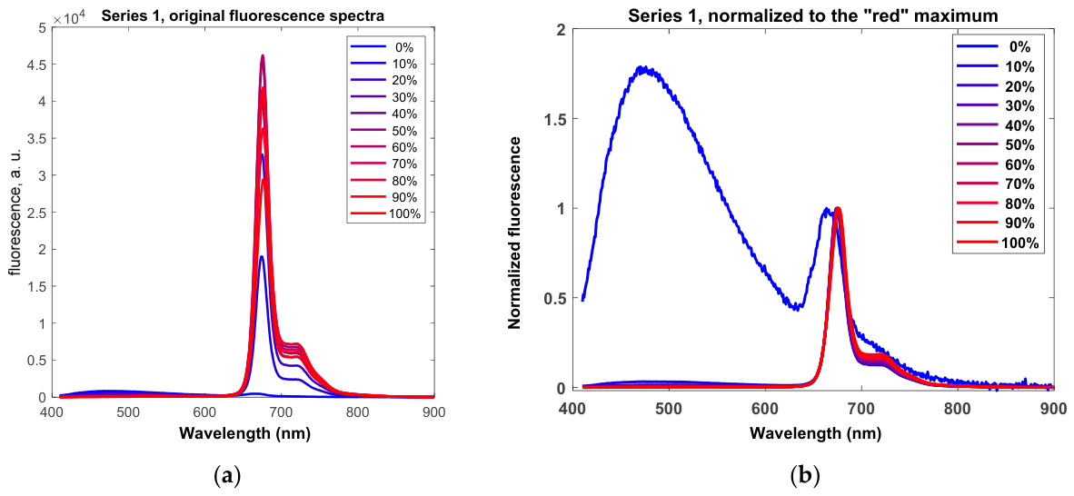
The data from the LIF spectra obtained from the spectrometer are illustrated in Figure 2a with the example of Series 1 and were used to assess the signal-to-noise ratio of the signal. Since each spectrum exhibits three characteristic regions, we estimated the S/N for each of them separately, relative to the signal at 250 nm, accepted as background signal. As can be expected, the lowest value for the S/N is for the 450–500 nm band, and for the smallest sunflower oil concentration, it is around 45, increasing to around 300 for the pure sunflower oil concentration. For the peak around 675 nm, it starts from 8000 and for the red plateau around 720 nm, it is above 1300.

Sunflower oil emission exhibits two main fluorescence bands. The one at 475 nm could be attributed to the fluorescence of tocopherols and tocotrienols, triglycerides and oxidation products. Kyriakidis et al. investigated the contribution of vitamin E to the fluorescence maxima at around 445–500 nm and concluded that it is negligible in comparison with the other fluorophores emitting in this spectral range [30]. Sunflower oils are usually classified with respect to the ratio of the triglycerides of oleic and linoleic acids. Typically, the most abundant one is linoleic acid, but oleic and minor presence of palmitic, stearic and other fatty acids is observed [31]. The emission in the red region is mainly due to the presence of chlorophylls and chlorophyll derivatives.

For the fluorescence of olive oil, the main fluorescence maxima at 675 nm and 720 nm arise from chlorophyll and pheophytins [19,32,33,34,35]. Although the peak around 675 nm, which has the highest relative intensity, dominates the spectrum, its absolute intensity significance for quantitative analysis is not unambiguous due to the inner filter effect [24,25].

The spectra are preprocessed as follows: First, the spectroscopy data outside the interval [410, 900] nm are discarded, mainly in order to exclude the disturbances from the laser itself. Thus, each spectrum consists of 643 datapoints. The spectral data are then normalized with respect to the maximum around 675 nm (the “red” maximum due to chlorophyll). Figure 2b shows the normalization output for Series 1 as an example. The “distortion” of the lightest-blue line in Figure 2b, corresponding to pure olive oil, is an artefact of the normalization with respect to the chlorophyll peak in the 675 region. Its absolute intensity as acquired from the spectrometer is much lower than the intensities of the OO-containing samples and it is barely visible near the abscissa of Figure 2a.

After the truncation and normalization operations, a “raw” dataset is built, each spectrum consisting of 643 datapoints (determined by the spectrometer wavelength sensitivity).

5. Neural Network Training Results

The training process can be organized based on training, validation and test sub-sets. It is also possible to organize the training process by feeding all data as a training subset and manually testing the trained NN with an additional (blind) test set after that. Ideally, with an ample and well-balanced number of datasets for the training process, one would split the input data into three groups: training, validation and method testing. The validation and testing groups are needed by the method in order to estimate the quality of the training process before additional blind tests. In the best scenario, these three groups should be independent but representative. For this reason, in order to start the training before obtaining a large amount of data, one needs other techniques for the internal validation and testing of the method. Therefore, we replicate by 100 the few datasets available by adding noise, which is Gaussian, and its amplitude and dispersion are frequency-dependent and are estimated on the basis of the measurement data. Then, we statistically pick 70% of the multiplied datasets for training, 15% for validation and the remaining 15% for internal testing, therefore ensuring that at least all three datasets are present in the training bunch. Such an approach would lead to two consequences: first, every run is biased depending on the 70% pick, and second, any new run would yield a slightly different result, since the 70% training data will be biased differently. This is permitted, because, as seen from Figure 2, the noise level is low and there is a clear trend in the spectral shape modification when the olive oil concentration increases. It should be also emphasized that with each new input dataset added, the bias decreases and once the training set is rich enough, the artificial multiplication approach is not necessary.

5.1. Informational Parameters with Biochemical Meaning (Diagnostic Parameters)

As was mentioned, a similar approach with one informational parameter, which is dependent on the concentration, has been used in other works. Tanajura da Silva et al. discuss the fluorescence intensity [26]; in [36], Yovcheva et al. analyze the refractive index; Nikolova et al. propose the blue peak detuning [19]; Torreblanca-Zanca et al. use the area under the fluorescence curve [24]. In our work, we apply a multi-parameter approach. The first parameter is the same used in [29], namely (i) the wavelength position of the red maximum. This parameter will be further denoted as C1 (criterion 1). In [29], this diagnostic parameter is the third one; so, for easier distinction, it will be denoted here as P3. 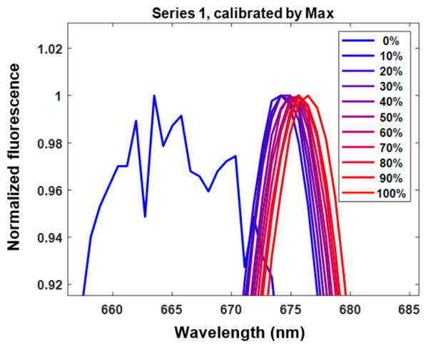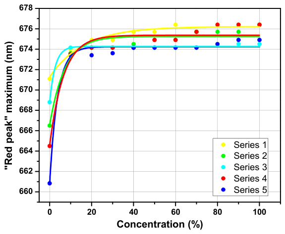Figure 3 presents a zoom of the red maxima region, where the dependence of the observed band position on the olive oil concentration is clearly seen. The behavior of this diagnostic parameter is shown in Figure 4. The figure also shows a large shift in the chlorophyll red peak position for the pure sunflower oil (the left-most curve) containing residual traces of chlorophyll and the much smaller but still noticeable shift with increasing the OO content in the samples. The larger relative noise in the sunflower oil curve with respect to the OO-containing samples is also a normalization artefact.

In Figure 4 above (as well as in Figure 5, Figure 7 and Figure 8 below) the solid lines are included for guiding the reader’s eye only, and are not related to the NN operation.

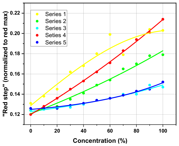
The second diagnostic parameter (ii) will be denoted as C2 and it is analogous to the second one used in [29] (we will use the notation P2), as only the reciprocal value is used. Thus, C2 is the amplitude ratio of the red “plateau” to the “red” maximum level around 720 nm, i.e., the level of the normalized “plateau”. Its concentration dependence is presented in Figure 5.

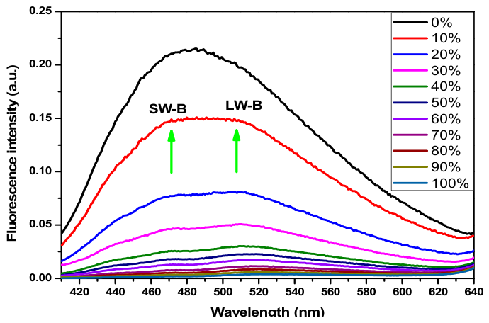
Regarding the blue-band region of the spectra, our measurements do not comply with the results obtained in [19] with respect to the lineshape of this band. The authors of [19] report a band with a clearly expressed single peak. Our measurements (a zoom is shown in Figure 6) show that a single peak is obtained only for the pure SO spectra (black line, not to scale with the other concentrations), while adding EVOO leads to a modification in its structure. As can be seen, the blue band is composed of two strongly overlapping broad sub-bands with maxima near 470 nm and near 515 nm. They form two distinct features, denoted by green arrows. Since the authors of [19] use excitation with 425 nm, we performed additional measurements using 425 nm excitation and confirm that the complicated structure of the blue band is still present. Due to the wavelength position of these two features, in the description, we will refer to them as “shorter- and longer-wavelength features of the blue band” or SW-B (the feature near 470 nm) and LW-B (the feature near 515 nm).

It can be seen that as a whole, the normalized fluorescence intensity level of this band decreases with concentration, while the relative levels of the features undergo a transition: the SW-B feature has a higher level at small concentrations and gradually the LW-B feature becomes predominant. In [29], the first diagnostic parameter used was the ratio of the intensity of the red maximum to the blue maximum (P1). This parameter would exhibit a jump when the blue band total maximum shifts from the SW-B to the LW-B. In order to take into account this behavior, here, we formulate the other two diagnostic parameters as follows:

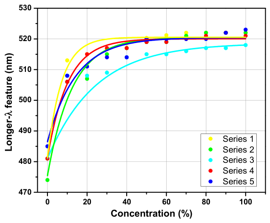
(iii) The wavelength position of the shorter-frequency feature (instead of the position of a single maximum of the blue band, which would lead to a “jump”), further denoted as C3;

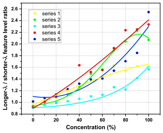
(iv) The ratio of the intensity levels of the LW-B to the SW-B features, referred to as C4.

For the automatic identification, the diagnostic parameters are determined through an analysis of the change in the slope of a fitting curve in three separate spectral regions (in order to avoid complicating the fitting model).

The introduction of these diagnostic parameters C1-C4 would facilitate the correct differentiation of a sunflower oil with a higher chlorophyll content from a mixture of sunflower and olive oil by taking into account the complex structure of the blue band. The dependence of the parameters C3 and C4 on concentration is shown in Figure 7 and Figure 8.

To assess the reproducibility of the spectral data, we performed a 10-fold measurement of each spectrum and estimated the standard deviation of the measurements and the standard error for each biochemical parameter. The maximal relative error obtained is 0.6% for C3 and 0.7% for C4, while for C2, the relative error is below 0.2%. With the resolution of our spectrometer, no deviation is obtained for C1. In the spectral areas of interest, the maximal absolute error for the family of representatives for a given concentration is more than three times smaller than the distance to the nearest representative of a family of another concentration. Thus, the measurement sensitivity and accuracy are high enough and are not expected to influence the classification accuracy.

Series 1 to 5 are extended by 100-fold multiplication to form a set of 3300 spectra for selection of training, validation, and internal testing sub-sets. For the concentration of 0%, there are no two peaks in the blue band area and parameter C4 is indeterminate. Therefore, as a first step, the program checks for coincidence of the wavelengths of the two blue structures (difference smaller than 3 nm). If they coincide, the corresponding curve is not analyzed further and is assigned to the ‘zero concentration’ class. If the difference is larger, the presence of olive oil in the respective sample is assumed. When constructing the calibration curves for C2, its value at zero concentration is assigned through extrapolation from the remaining points. This does not affect the classification of pure sunflower oil since it is classified at the preliminary stage. This approach supports the training process by providing an unambiguous and continuous curve. Another possible approach would be to introduce a hard limit in the process of NN training. For nprtool (classification), a grid with 5 hidden neurons and conjugated gradient training was used. Then, in the recognition process, the “center of gravity” of the probability vector is estimated in order to convert the classification into estimated concentration.

5.2. Classification Approach

With this approach, we solve the problem as a classification task (equivalent to pattern recognition) in 11 discrete classes (of percentage of the olive oil). Then, the probability of belonging to a given class could be fitted to some smooth function, if needed.

For building, training and testing the NN, the MATLAB R2022b nprtool interface app from MATLAB Deep Learning Toolbox is used [37]. The nprtool is an interface to the patternnet function from the same toolbox. This is the recommended function for creating neural networks for tasks related to pattern recognition. It creates a two-layer feedforward NN with sigmoid hidden neurons and softmax output neurons, suitable for classification, as described in the Deep Learning Toolbox documentation. The NN is trained using the scaled conjugate gradient method. The performance at every iteration is evaluated by the cross-entropy criterion. The training is stopped after the validation criterion is met, i.e., the cross-entropy does not decrease anymore in this case.

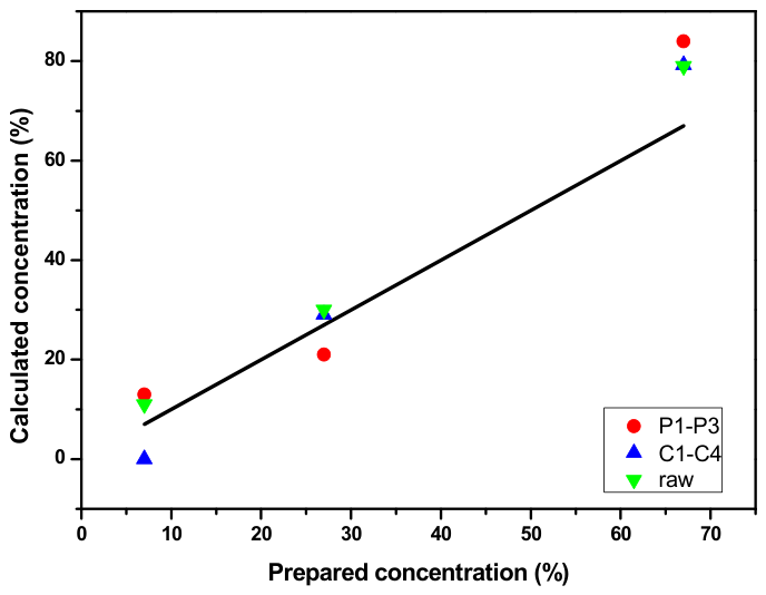
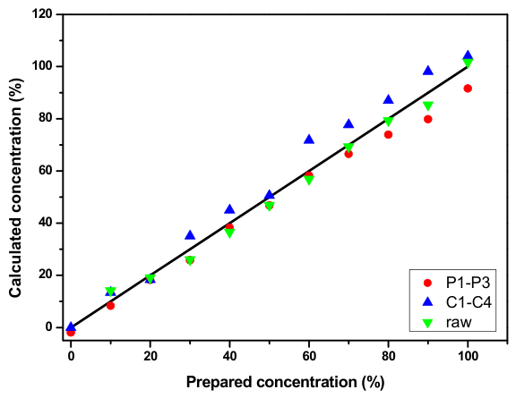
The results obtained for the classification of the test series using the diagnostic parameters C1–C4 (which account for the complex shape of the blue band) are shown in Figure 9 (for Series T1) and 10 (for Series T2). Since the input in this case is a four-parameter one, the corresponding data are marked in the figures as “C1–C4” (blue dots). For easier comparison, we add the results reported in [29] for the three-parameter training (considering the blue band as having a single structure, red dots denoted as “P1–P3”) and for the raw data (green dots, denoted“raw”). In the figures, the dots mark the predicted vs. the prepared concentration for the blind testing. The values for the predicted concentrations are calculated as the sum of the output concentrations weighted by the corresponding probability. For clarity, the black line in the figures denotes the 45% line for ideal prediction. The results from the blind tests with series T1 (Figure 9) are relatively similar to the ones obtained in [29]; probably, initial signs of overfitting are observed in this case. As regards the T2 samples (Figure 10), we see a noticeable improvement, as the blue dots corresponding to the present four-criterial approach lie much closer to the ideal 45-degree line.

If the training sets are more diverse and representative, the training process should be able to manage to distinguish such deviations.

5.3. Fitting Approach

The task here can also be naturally formulated as an NN fitting task between the data and the percentage of olive oil. It is known that a fairly simple neural network can fit any practical function. The classification approach described above shows that the four parameters with biochemical meaning C1-C4 yield enough information about the mixture ratio; so, we take them as input data.

The training set here is again built on the data from Series 1 to 5. For the building, training and internal testing of the NN in this case, the MATLAB R2022b nftool interface app from the MATLAB Deep Learning Toolbox was used [37]. It is an interface for the fitnet function, which solves tasks for NN fitting using shallow two-layer feed-forward neural networks. The Scaled Conjugate Gradient is standard for NN training; it is memory-efficient and uses gradient calculations. The best for small or noisy datasets is the Bayesian Regularization, as it minimizes a combination of squared errors and weights to improve generalization.

We used a grid with four hidden neurons and Bayesian regularization to reduce the error in the final concentrations. After several runs, the optimization criterion is met (validation performance evaluated by the reached minimum of the gradient of the mean square error). The early stopping method is applied to improve generalization and avoiding the overfitting of the NN.

The trials show that more than five hidden neurons seem to be unnecessary and will probably tend to overfitting because the data are not too diverse.

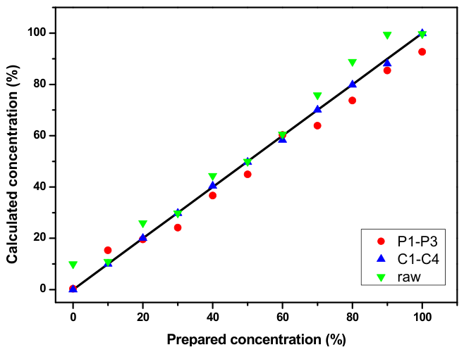
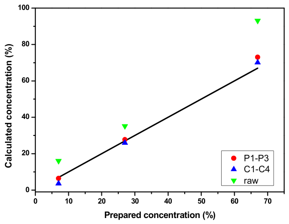
The blind test results regarding the predicted proportion of the olive oil are shown in Figure 11 for the T1 series and in Figure 12 for the T2 series. Unlike the first approach that yields probabilities for belonging to a given class, the results here are numbers corresponding to the predicted concentration of olive oil. Again, here, we compare the performance of neural networks trained with the four diagnostic criteria C1–C4, defined in the previous chapter (blue dots, “C1–C4”) with the output of the training with the raw spectral data (green dots, “raw”) and with the three-criterial approach (red dots, “P1–P3”) obtained in [29].

Here, the plot in Figure 11 and Figure 12 also includes a line marking the 45° ideal output. As with the classification approach, the results from the T1 series testing based on the criteria C1–C4 are similar to the ones obtained in [29]. The raw data output for the T1 series shows that the model tends to overfit; thus, the results for the T2 calibration are clearly better. We should note that, in Figure 12, we excluded the results of the raw data for the pure sunflower oil, since it is misidentified. Most probably, this is due to the fact that the SO samples contain a non-negligible chlorophyll residue. For the T2 series testing, the four-criterial approach yields a slight over-estimation, while the three-criterial approach performs better at lower concentrations and yields a slight under-estimation for the higher EVOO concentrations. Probably the C1–C4 criterial approach would perform better when additional representative data are added. It should be noted again that for the reliable operation of the Bayesian regularization, a lot more data are preferable.

6. Discussion

In the present work, we have shown the possibility for identification and classification of mixtures of extra-virgin olive oil and sunflower oil based on fluorescence spectra induced by laser excitation at 405 nm. Although, from the raw data, one might suppose that a single parameter extracted from the spectra could be sufficient for calibration tasks, our results do not support such assumption. As was mentioned, the intensity of the chlorophyll peak itself [23] is an ambiguous criterion due to the inner filter effect (re-absorption of fluorescence). The wavelength of the blue band maximum used as a criterion in [19] would yield a jump in the parameter dependence on concentration for complex lineshapes, as is the case for certain samples. Such a jump would also be susceptible to incorrect automatic maximum determination due to noise. Moreover, in small-sample scenarios, a single criterion might turn out to be not representative for a large class of samples. Therefore, for complex samples, either the full spectrum, or the multi-criterial approach is preferable.

Here, we define four information parameters with biochemical meaning C1–C4 and determine their behavior with respect to the mixture concentration. We show that these parameters have different sensitivity in the different concentration ranges, which could improve the identification results. We combine laser-induced fluorescence spectroscopy and NN machine learning, where the spectral data are used as input for the training of the NN and its performance is assessed by testing both with modified samples data from the training sets and with data that are new to the algorithm. The modified samples include intermediate concentrations in order to check the NN performance towards overfitting.

Since the data used for training are insufficient, we perform 100-fold replication with addition of noise to form a bunch for statistically selecting 70% for training, 15% for validation and 15% for the method testing. In principle, these three groups should be independent and representative, but in order to start the training before obtaining a large amount of data, one needs other techniques for the internal validation and testing of the method. This approach could be beneficial for iterative testing and optimization of the NN during the process of data collection. The bias, inherent to this approach, would decrease with each new sample added, and when enough data are collected, replication is no longer necessary.

Our preliminary results from NN training show that, in principle, the task of concentration recognition could be approached both as a classification and as a fitting problem. The classification approach is equivalent to fuzzification of the concentration into discrete classes, while the fitting approach is more natural in this case.

It should be noted that the classification and fitting strategies are in general applicable to different tasks. For the particular case described in the present work, both are possible, but, for example, for tasks related to origin, variety or producer determination, as well as for optical biopsy based on spectral data and ML [38], the task is purely classificational. On the other hand, other tasks are inherently calibrational (e.g., concentration determination) and, for them, the fitting approach would be more appropriate. In both cases, the proper choice of diagnostic parameters is important, as well as the formulation of strategies for preliminary work when there are still insufficient data for complete analysis.

From the concentration dependence of the diagnostic parameters, it can be seen that each parameter is more sensitive in different concentration ranges. For example, the intensity ratio criteria (C1 and C3) are more or less equally sensitive in all concentration regimes, while the wavelength-related criteria C2 and C4 are linear up to 15–25% concentrations and further tend to saturate (with similar values for very different concentrations).

It is useful to compare NN classification capability not only in terms of the weighted average of the predicted concentrations, but also with respect to the spread of the probabilities of classification into different classes.

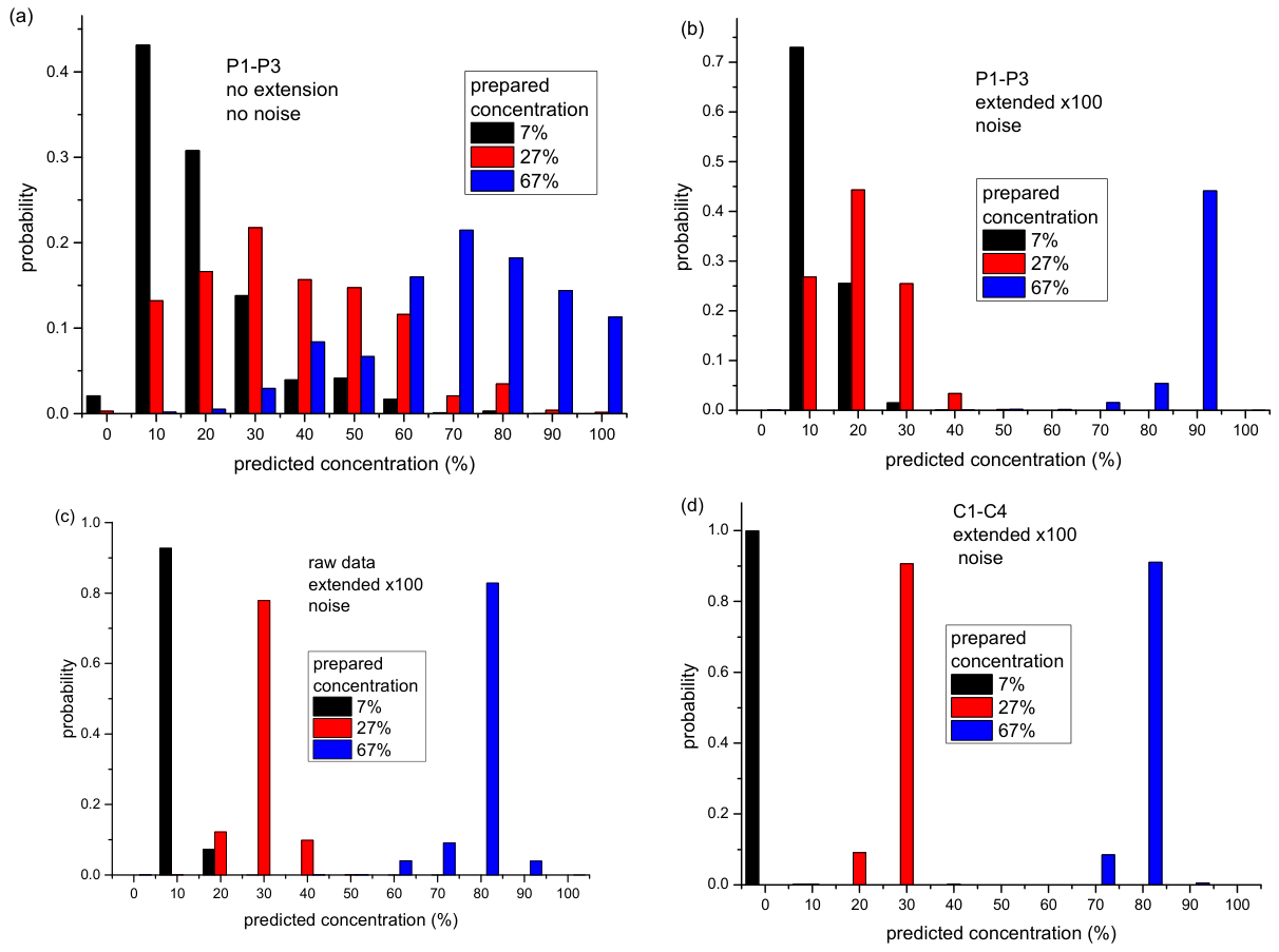
Figure 13 presents a comparison of the classification output for the following four cases. The first three (Figure 13a–c) are based on the tabular data given in Figures 2–4 of [29], while Figure 13d reflects the data corresponding to the approach used in the present work. Figure 13a is included for comparison of the output when the datasets are not augmented, while 100-fold augmentation with addition of noise is applied for the results in Figure 13b–d.

The information in Figure 13 gives insight into the spread of the probabilities for classification of the samples from Series T1. In the histograms, the black, red and blue bars are the probabilities determined using the different approaches for classification of the 7%, 27% and 67% samples of Series T1. Figure 13a shows the probability spread when the NN is trained only with the parameters P1–P3 determined from the normalized spectra without dataset extension. For a very rough estimation, the spread could be assessed by the standard deviation of the measurements. Figure 13b is the spread when criteria P1–P3, described in [29], are applied to the 100-fold extended datasets with addition of noise. For this case, the spread is reduced by more than two times. Figure 13c is also based on the data in [29], only for the case of NN training with the full normalized spectra (i.e., the raw data, extended with noise), and the spread is reduced four times compared to the first case. Finally, using criteria C1–C4 applied to the extended with noise spectra, we obtain almost a six-time reduction in the spread, as illustrated in Figure 13d.

Thus, the present results might suggest a comparable performance of the NN with raw data training and training with biochemical diagnostic parameters. Better results from raw data training (compared to the criterial approach) have been reported in a recent work where the two classification approaches have been applied for classification of different types of skin tumors by means of supervised e-learning using fluorescence and reflectance spectra [38]. It is important to note, though, that both in the present work and in [38], the input training data are too few. Therefore, a general conclusion on the advantages of one of these approaches cannot be drawn, although the overfitting in the last approach is expected to decrease to some extent with increasing the number and diversity of the data. Nevertheless, our results show that these methods perform well even with very scarce data. Further work in expanding the database for training sets with more samples from different producers is in progress. A sufficiently large dataset would make it possible to compare the NN performance with classical methods like PLS, SVM or PCA, where the significance of each criterion could be estimated and weights of the criteria can be specified more precisely, even though this step is not necessary when utilizing NN training.

In the initial processing of complex spectra with an insufficient number of samples, it is possible to make a preliminary assessment of the significance of the predictors by creating a decision tree with Bayesian optimization based on the full-spectrum data. This would provide information on the importance of the fluorescence intensities in the different spectral regions. Such estimation is in progress and the preliminary results show that the most informative is the region around 420 nm, followed by the region around 640 nm and around 740 nm. This information could be a basis for the formulation of diagnostic parameters, whose significance is to be assessed as a further step. This could be an iterative process both for the selection of diagnostic parameters and with the accumulation of new data.

Although, in the present case, the NN is applied only for two-component diagnostics, it creates a solid background for further improvement in the methodology to deal with more complex mixtures. Since such biological samples are complex, they can vary depending on their origin, producer (processing technology), specific year of production, aging, etc., and a lot more diverse data are needed in order to test model robustness against such deviations and its capabilities for classification with respect to them. Currently, work is in progress on the application of the described approaches on another type of potable samples, for which the number and diversity is much larger and would be representative for such analysis. The development of NN could create useful tools for automatic control of various products, bearing in mind that the adulteration of products is becoming more and more sophisticated.

7. Conclusions

For specific applications related to composition analysis based on spectroscopic measurements, it is both expensive and time-consuming to perform a large number of measurements. Preliminary selection of diagnostic parameters (if properly chosen) makes it possible to achieve similar results with a smaller number of measurements. Even if, in some cases, a single criterion appears sufficient when examining a small number of samples, a sample from a different manufacturer, origin, etc., with a different spectral structure, may be strongly misdiagnosed. On the other hand, although, with a sufficient amount of data training with raw data, it is expected to perform well, to some extent, it would function as a black box without providing information for biochemical interpretability and analysis. Therefore, an appropriate approach could be to apply a multi-criterial approach and evaluate the significance of the predictors (both the individual spectral points in the case of raw data, and the formulated diagnostic criteria). This could indicate among which frequencies it is appropriate to formulate criteria without overlooking a criterion of high significance.

The correct choice of appropriate diagnostic parameters is of importance from the point of view of biochemical interpretability and analysis and for improved generalization in small-sample cases, whereas the “black box” full-spectra training might be beneficial for end-user applications. The use of normalized spectra as input has the advantage of easier data transfer between different registration and measurement devices.

It should also be noted that the need for easy-to-operate, compact, low-consumption ON-OFF devices, although with lower-grade performance, is not negligible from an economic point of view. Diode-laser-based spectrometers offer such an option in terms of hardware. The portable in situ use of such devices could offer a pre-selection of suspicious samples for further advanced analysis, leading to a considerable cost reduction.