


Abstract
This study presents a performance-based forensic investigation of the Tanada wall, a geosynthetic reinforced soil wall with a full-height rigid facing that experienced strong shaking during the 1995 Hyogoken Nambu earthquake in Japan. The analytical framework integrates a compiled soil stress–displacement dataset, limit equilibrium constraints, displacement-based back analysis, reconstruction of the displacement (Δ3h)–seismic inertial coefficient (kh) curve, and systematic parameter sensitivity evaluation. The displacement-based seismic resistance curves developed using representative soil parameters show that the Tanada wall maintains strong seismic resistance up to HPGA ≈ 0.7–0.8 g, with displacement trends that remain physically consistent across three logarithmic cycles. Sensitivity analyses demonstrate that only three parameters—the soil stiffness number K, peak friction angle φpeak, and the initial pullout stiffness number Kt—produce variations of approximately ±0.8–1.5 × 10⁻³ m in the final displacement Δ3h. All remaining soil, reinforcement, and facing parameters contribute only minor variations on the order of a few 10−4 m. These findings show that the force-equilibrium-based finite displacement method (FFDM), supported by laboratory evidence and displacement-based inference, provides a rigorous and physically grounded methodology for forensic evaluation of reinforced soil structures.
1. Introduction
1.1. Motivation for Performance-Based Forensic Geotechnical Evaluation
Interpretation of observed geotechnical structural behavior, reconstruction of governing failure mechanisms, and evaluation of mobilized strength form the core of forensic geotechnical evaluation, where lessons from past performance are used to improve design and assessment. Conventional practice has emphasized identifying causes of failure and refining design methods through data collection, interpretation, and analysis, allowing previously overlooked factors to be incorporated into updated guidelines. However, even with such updates, the seismic performance of redesigned structures often remains uncertain. This is illustrated by the forensic investigation of a caisson failure reported in [1], in which liquefaction of foundation soils and wave-induced thrusts were identified as the primary causes. Although such mechanisms can be incorporated into revised provisions, the resulting structural performance remains unknown because safety continues to be evaluated using the limit equilibrium-based safety factor Fs. This scalar index provides only a binary definition of failure at Fs = 1.0 and offers no insight into deformation demand or failure progression. Leonards [2] defined failure as an unacceptable difference between expected and observed performance, underscoring the need for performance-based evaluation procedures in geotechnical design and forensic activities. This forms the central motivation of the present study.
1.2. Analytical Framework: From LEM to FFDM
A performance-based approach to forensic geotechnical evaluation is developed in this study, in which the force-equilibrium-based finite displacement method (FFDM) plays a central role. The FFDM extends the traditional limit equilibrium method (LEM) by enabling analytical computation of displacements for a wide range of failure mechanisms, including circular, noncircular, arbitrary, and multi-wedge modes [3,4]. This displacement-based capability allows forensic interpretation to be directly linked to performance-based seismic evaluation, thereby bridging the gap between observed behavior, back-calculated parameters, and forward-looking design assessment.
1.3. Failure Mechanisms in Reinforced Soil Structures
In both the LEM and FFDM analyses, incorporating a representative failure mechanism is essential for interpreting the behavior of reinforced soil structures. This requirement is particularly important for interaction-rich systems such as the Tanada geosynthetic-reinforced soil wall, where coupled soil–reinforcement and reinforcement–facing interactions commonly lead to compound or multi-wedge failure patterns. Early reinforced-soil research, beginning with Vidal’s pioneering work on Reinforced Earth, showed that reinforced backfills tend to deform as a coherent block bounded by a two-wedge (or bi-linear) failure mechanism [5,6]. Subsequent field observations and analytical studies [7,8,9,10] demonstrated that reinforced soil masses frequently mobilize multi-wedge internal failure mechanisms rather than a single planar failure surface. Large-scale model tests and full-scale monitoring programs conducted by Tatsuoka and co-workers in the 1980s–1990s [11,12,13,14,15] confirmed that bilinear or multi-wedge failure surfaces commonly develop under monotonic and seismic loading. These cumulative findings also demonstrated the structural stabilizing function of the facing, establishing it as an essential component in the design process [16]. This body of work further fostered the development of the prototype multi-wedge failure mechanism [17], which explicitly incorporates the facing as an integral part of the failure-wedge system for a unified stability assessment. The multi-wedge mechanism adopted in the present study, implemented in SLOPE-ffdm 2.0 [18], is an extension of the formulation proposed in [3,4], updated to include the enhanced features of the FFDM framework.
1.4. Role of Back Analysis in Forensic Geotechnical Engineering
Back analysis has long been a central component of forensic geotechnical engineering because it enables soil and interface properties to be inferred from observed states. Formalized procedures for slopes, foundations, and retaining structures have demonstrated how field performance can be inverted to obtain realistic strength and stiffness parameters [19,20]. Numerous studies on slope failures have shown that LEM-based back analysis provides a practical means of identifying a plausible range of soil strengths, owing to the universal force-equilibrium principles embedded in LEM [21,22,23]. This role of LEM is foundational and complementary to displacement-based back analysis. In the present study, the LEM and the FFDM are applied jointly to back-calculate mobilized strength and deformation parameters, forming the basis for establishing displacement-based seismic resistance curves that support assessment of reinforced soil structures. Following the 1995 Hyogoken-Nambu earthquake, the investigations reported in [24,25] performed LEM-based back analysis for the critical seismic coefficient khc to re-evaluate the pseudo-static conversion factor η, defined as:
where HPGA is the horizontal peak ground acceleration and g is the gravitational acceleration. By comparing back-analyzed values of η for various damaged retaining walls, they showed that conventional gravity and leaning walls typically correspond to η values near 0.6, whereas reinforced soil walls such as the Tanada wall likely exhibit a lower value of η due to soil–reinforcement-interaction-induced flexibility (or ductility) of the reinforced soil system.
η = khc/(HPGA/g)
1.5. Limitations of Existing Seismic Evaluation Methods
Current design manuals for mechanically stabilized soil walls (or reinforced soil walls), including the Federal Highway Administration (FHWA) guidelines [26,27,28] and the National Concrete Masonry Association (NCMA) manual [29], adopt a two-wedge mechanism to evaluate the external stability of the coherent block, which comprises the facing and the reinforced zone behind it. Throughout the design process, the reliance on multiple safety factors for different failure modes and loading conditions results in an uncertain overall performance of the designed structure. With respect to seismic behavior, these guidelines do not provide a direct means of determining the critical seismic coefficient required for displacement evaluation using Newmark’s method [30,31,32,33]. The FFDM, incorporating multi-wedge failure mechanisms, addresses these limitations by generating displacement-based seismic resistance curves that quantify the deformation capacity of the reinforced soil system over a range of seismic coefficients. When combined with site-specific seismic demand, these curves support performance-based evaluation of reinforced soil structures.
Silva et al. [34] attributed the safety of geotechnical structures to the overall quality of design, construction, and operation. Based on safety factors for 75 projects across a wide range of geotechnical facilities, they derived annual failure-probability–Fs relationships for facilities with different quality levels. Construction-related issues identified in forensic investigations, such as inadequate subsurface characterization, improper sequencing, and drainage deficiencies [35,36], further highlight the need for integrated assessment. Probability-of-failure–Fs curves have been used to identify the primary cause of the Finneidfjord landslide in Northern Norway [37,38], demonstrating the value of probabilistic interpretation. Geomaterial variability has been treated as a key factor affecting the acceptability of geotechnical structures and a preliminary probability-based criterion was proposed in [39]. Despite their advantages, these probabilistic approaches remain tied to the limitations of LEM—the absence of performance-based or displacement-based analysis. These studies collectively underscore the need for a comprehensive performance-based forensic framework.
Performance-based evaluation requires comparing seismic demand with deformation capacity, but pseudo-static kh–kv analyses do not compute displacement and therefore cannot support this comparison. Recent advances in displacement-based assessment, including the development of seismic resistance curves [40], provide a more realistic means of characterizing how retaining structures and slopes respond to strong shaking. A seismic resistance curve is analogous to the monotonic pushover curve used in structural engineering, which characterizes the system’s lateral force–deformation capacity. The proposed curve expresses the displacement–lateral force relationship by plotting displacement (Δ) against the equivalent lateral force represented by kh and kv, effectively serving as a reciprocal form of the conventional base shear–drift pushover representation [41,42,43].
1.6. Distinctions Between This Study and the Previous Investigation
Although the background theory of the seismic resistance curve and the analytical framework are the same as those used in [40], the present study addresses several aspects that have not been previously examined.
- (1)
- The forensic site of the Tanada wall is a GRS-FHR wall, fundamentally different from the GRS wall with modular-block (MB) facing analyzed in [40]. The full-height rigid (FHR) panel provides a structural stabilizing function distinct from the stacked block column, generating a more effective “coherent gravity” block within the backfill. Consequently, the failure mechanisms of a wall with a rigid facing differ substantially from those of a wall with a stacked block facing.
- (2)
- The Tanada wall was subjected to very strong to extreme ground shaking, with HPGA = 0.7–0.8 g, a level rarely documented for GRS walls. Despite the unusually high seismic demand, the wall exhibited only moderate deformation (Δ3h ≈ 0.1 m), demonstrating exceptional seismic resistance. In contrast, although the modular-block walls examined in [40] were subjected to only moderate shaking (HPGA ≈ 0.45 g), one of the investigated walls nevertheless reached a collapsed state, exhibiting lateral buckling of the facing with a displacement exceeding 0.47 m.
- (3)
- Extensive subsurface exploration was conducted in [40], and soil properties were identified using disturbed and undisturbed sampling, standard penetration tests (SPT), and laboratory direct shear tests. For the Tanada wall, however, the available backfill information is comparatively limited, with only a small number of laboratory test results reported from the post-earthquake investigation. To address this limitation, a dataset of direct shear tests covering a wide range of soils is introduced to support the identification of representative soil parameters. The combination of this direct shear dataset and displacement-based back analysis represents a new element in forensic geotechnical investigation, enabling soil parameter estimation even when site-specific data are limited.
1.7. Scope of the Present Study
In geotechnical applications, a displacement-based seismic resistance curve provides two essential functions: it verifies observed deformation against analytically reconstructed behavior and enables forward prediction of structural performance once a seismic demand is specified. Past forensic geotechnical practice has lacked a unified means of linking observed behavior, mobilized strength, and predicted deformation, and the FFDM framework developed in this study addresses this gap by establishing displacement-based seismic resistance curves that define the deformation capacity of reinforced soil structures over a range of seismic coefficients. When site-specific demand is specified, these curves provide a consistent basis for performance-based evaluation. The scope of this study is limited to the technical mechanisms and analytical procedures relevant to forensic geotechnical evaluation; broader procedural, organizational, and legal aspects of forensic engineering are not addressed.
2. The Forensic Site: The Tanada Wall
The Tanada wall is a GRS-FHR wall forming part of a railway embankment for the JR Tokaido Line. It is located in an area that experienced severe shaking during the 1995 Hyogoken-Nambu earthquake (also referred to as the Kobe earthquake; ML = 7.2). The wall was situated within a region assigned a Japan Meteorological Agency (JMA) seismic intensity of 7 [24] (on a full scale of 10; reached only seven times in Japan’s recorded history), as shown in Figure 1. Based on field observations and one-dimensional seismic response analyses, an HPGA ≈ 0.7 g at the Tanada wall site was estimated in [24]. An even higher estimate of HPGA in the vicinity of the wall, possibly reaching 0.8 g with a negligibly small vertical-to-horizontal acceleration ratio λ, was also reported in [25]. By comparing the wall at completion (Figure 2) with its condition during the post-earthquake investigation (Figure 3), it is evident that despite extensive damage to nearby houses (approximately 50% complete collapse of wooden houses) and to various soil-retaining structures, the Tanada wall exhibited high seismic resistance during the earthquake.
Figure 1.
Location of the Tanada wall (compiled from [24]).
Figure 2.
The Tanada wall at completion (courtesy of Dr. M. Tateyama).
Figure 3.
The Tanada wall after the earthquake (courtesy of Dr. M. Tateyama).
Post-earthquake measurements indicated horizontal displacements of 0.1 m at the toe (i.e., observed Δ3h = 0.1 m) and 0.26 m at the top, as illustrated in Figure 4. The 0.2-m-wide H-piles located behind the wall, spaced at 1.5 m and installed without lagging, were excluded from the analysis because their slender geometry, wide spacing, and shallow embedment provide only negligible resistance to lateral earth pressures. According to Ito and Matsui’s theory [44], soil arching collapses when pile spacing exceeds approximately 6–8 pile diameters, resulting in negligible lateral thrust on the piles. The Tanada wall piles have a center-to-center spacing of 1.5 m and a clear spacing of 1.3 m, corresponding to more than seven pile diameters, indicating that they do not intercept active thrust. A conservative assumption of 10% thrust interception corresponds to reducing Ka from 0.217 to 0.195, equivalent to a friction-angle change of approximately 2°. As shown later in the sensitivity investigation, variations of this magnitude in ϕ have only a minor influence on the computed displacement. Therefore, the H-piles are omitted from the FFDM analysis because their lateral resistance is negligible and does not affect the translational displacement Δ3h.
Figure 4.
Cross-section of the Tanada wall following the earthquake.
The Tanada wall was constructed using high-quality, cohesionless backfill (cpeak = 0) under the supervision of the Japan Railway Technical Research Institute [16]. The reinforced concrete facing has a total height of 5.8 m, with thicknesses of 0.5 m at the base and 0.3 m at the top. The reinforcement consists of woven PVA (polyvinyl alcohol) geogrids with a nominal longitudinal tensile strength of 30 kN/m, placed at a vertical spacing of 0.3 m and embedded 2.5 m into the backfill, with every fifth layer extended to 3.0 m. Additional reinforcement properties related to creep and construction damage were thoroughly investigated in [16]. The assumption of λ = 0 for the Tanada wall is supported by the study in [45], in which analysis of the seismograph record at the JMA Kobe station (HPGA = 0.82 g) indicated λ = 0.058 at the moment of HPGA. Another seismograph at the Higashi-Nada station, located approximately 2 km from the Tanada wall, recorded HPGA = 0.42 g in the N–S direction during the earthquake. Although this represents a less likely shaking scenario for the Tanada site, it remains a possible alternative. A value of λ = 0.383 at the moment of HPGA was also reported in [45] based on the Higashi-Nada record. Therefore, an earthquake scenario with HPGA = 0.42 g and λ = 0.4 is considered in this study as a plausible, though secondary, seismic input condition.
Post-earthquake sampling and triaxial testing indicated a peak internal friction angle of φtriaxial = 42° for the retrieved backfill soil [24]. To estimate the corresponding φpeak under a plane-strain condition representative of the in situ embankment, a modest enhancement factor of 1.11–1.14 was applied to the triaxial value, consistent with experimental evidence showing that peak strengths in plane strain exceed those in axisymmetric compression by several degrees for dense sands [46,47]. This yields an estimated φpeak = 47–48° as the upper-bound peak strength for the Tanada wall backfill. The internal friction angle at the residual or steady-state condition, φres, inferred from triaxial, plane-strain, and direct shear studies on sands [48,49,50,51,52], is typically on the order of 0.8–0.9 of φpeak at comparable stress levels, corresponding here to φres ≈ 38–43°. It is noted that an operational friction angle of φ = 40° has been adopted in the JRTRI design guideline [16] as an upper-limit design value for earth structures, including both reinforced and non-reinforced embankments, and the same value of φ = 40° was used in the post-earthquake stability analysis reported in [24].
3. Analytical Method
This section summarizes the core components of the FFDM formulation and its implementation in [18]. The FFDM-based displacement analysis incorporates four essential elements: (1) a representative multi-wedge failure mechanism appropriate for the structure under consideration; (2) force equilibrium combined with a hyperbolic stress–displacement model; (3) a post-peak stress–displacement formulation for capturing softening behavior; and (4) displacement compatibility between adjacent wedges or slices. The presentation below focuses on the conceptual framework relevant to the forensic analysis.
3.1. Multi-Wedge Failure Mechanism
Figure 5 illustrates the multi-wedge failure mechanism (Type-4 failure mechanism in SLOPE-ffdm 2.0) adopted in this study. The mechanism consists of two active wedges (Wedges 1 and 2), a facing column (Wedge 3), and a passive wedge located in front of the facing toe (Wedge 4). Trial failure surfaces are generated through a systematic trial-and-error procedure based on predefined matrices of control points 1, 2, and 3 (Figure 5). For the Tanada wall, control point 3 is fixed at the heel of the facing because a through-facing failure surface is physically precluded by the reinforced concrete facing, which has a thickness of 0.3–0.5 m. A total of 5389 trial surfaces are generated for each analysis case, and the FFDM is applied to compute the corresponding displacements Δ1 through Δ4 along each candidate failure surface. The critical surface is defined as the one producing the maximum crest settlement Δ0 for the specified input parameters. In the following, Δ3h is used throughout to represent the horizontal displacement of the facing.
Figure 5.
Schematic illustration of the multi-wedge failure mechanism used in the FFDM.
The multi-wedge failure mechanism in the FFDM represents a translational deformation mode of the reinforced backfill, consistent with experimental evidence and post-earthquake observations at the Tanada wall. The reported 0.26 m top displacement reflects a rotational movement of the rigid facing, which is outside the kinematic scope of the FFDM and therefore unsuitable as a calibration target. In contrast, the toe displacement Δ3h directly corresponds to the translational movement of Wedge 3 and is minimally influenced by facing rotation or post-shaking adjustments, making it the most reliable and physically consistent quantity for displacement-based back analysis.
3.2. Hyperbolic Soil Stress–Displacement Model
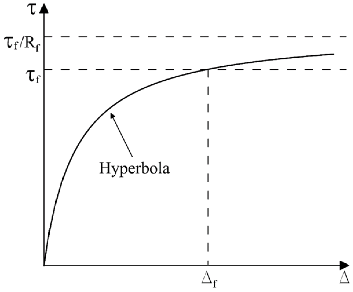
The central feature of the FFDM is the iterative coupling between force equilibrium and the hyperbolic stress–displacement relationship. As illustrated in Figure 6, the hyperbolic model describes the normalized shear stress (τ/τf)–shear displacement (Δ) response along the potential failure surface:
where
τ/τf = ∆/(a + b × ∆)
- a = τf/kinitial
- b = Rf
- kinitial: initial shear stiffness of soils;
- τult: asymptote strength at infinite displacement;
- τf: shear strength of soil according to the Mohr–Coulomb failure criterion;
- Rf: failure ratio (=τf/τult).
The shear strength of soils (τf) is defined by the Mohr–Coulomb failure criterion:
τf = cpeak + σ′n × tan φpeak
- σn′: effective normal stress;
- cpeak: peak cohesion intercept at failure;
- φpeak: peak internal friction angle of soils.
Figure 6.
Hyperbolic normalized shear stress–displacement curve used in the FFDM.
Equation (2) can be interpreted as a reciprocal formulation of the local safety factor FSi at the base of the soil block (or slice) i:
τf, i, τi: shear strength and stress, respectively, at the base of soil block (or slice) i
FSi = τf, i/τi
The initial shear stiffness kinitial is given as a power function of effective normal pressure:
kinitial = K × G × (σ′n/Pa)n
- K: initial shear stiffness number (dimensionless)
- Pa: atmospheric pressure (=101.3 kPa)
- G: reference shear stiffness (=101.3 kPa/m)
- n: pressure dependency exponent
In the FFDM, the iterative calculations for force equilibrium and the hyperbolic stress–displacement relationship are performed sequentially for Wedges 1 through 3 (or 4, if present). Iterations continue until the boundary force at the left side of Wedge 4 falls below the convergence threshold of 0.1 kN/m. Details of the computational algorithm are provided in [40]. The use of the term “force equilibrium” emphasizes that FSi (as defined in Equation (4)) varies along the slip surface and is not constrained to be constant, distinguishing the FFDM from conventional limit equilibrium formulations.
3.3. Post-Peak Stress–Displacement Relationship
The hyperbolic formulation in Equation (2) describes the pre-peak and peak portions of the shear stress–displacement response. To capture the softening behavior that follows peak strength, the FFDM incorporates a post-peak stress–displacement model that reduces shear resistance as displacement increases beyond the peak value. The post-peak branch is represented by a classical curve known as the Versoria or Witch of Agnesi, governed by the residual friction angle (φres) and the peak-to-residual displacement ratio (Δratio). This post-peak representation is essential for realistic simulation of reinforced soil structures subjected to strong shaking, where large displacements can develop along portions of the failure surface. A prototype of this model for analyzing a landslide with a prescribed failure surface was presented by [53], indicating that incorporating post-peak soil behavior improves the accuracy of slope displacement predictions. The refinement of the formulation to better reflect geotechnical practice in capturing the residual state of soils was reported in [40]. A detailed description of the post-peak model is provided in [40], and its implementation in SLOPE- ffdm 2.0 follows the same framework.
3.4. Displacement Compatibility
The compatibility function expressed in Equations (6) and (7) is derived from the hodograph (displacement diagram), which enforces displacement compatibility along the failure surface, as schematically illustrated in Figure 7. This function serves two purposes: (1) satisfying the kinematic requirements of a deforming soil mass, and (2) relating the ns unknown displacements (Δi, i = 1 – ns) to the slice-base inclination angle (αi) and the average dilation angle along the slip surface (ψ). For any potential failure surface, the compatibility function reduces the n displacement variables to a single unknown, ψ, which can be empirically determined from the mobilized dilation behavior along the slip surface. As shown by [53,54], a positive ψ indicates volume expansion along the failure surface and generally produces an increasing-toward-toe displacement pattern, whereas a negative ψ corresponds to volume contraction and results in a decreasing-toward-toe displacement distribution. This compatibility condition ensures that the multi-wedge mechanism deforms coherently and that the computed displacements reflect a physically admissible deformation mode.
Δi = Δ0 × f (Δi)
f (Δi) = cos (α1 − 2ψ)/[sin (α1 − ψ) × cos (2ψ − α1)]
Figure 7.
Displacement compatibility conditions between adjacent soil blocks in the multi-wedge failure mechanism.
4. Material Properties and Constitutive Models
4.1. Direct Shear Test Dataset
To establish preliminary bounds for these parameters, seven series of direct shear tests [55,56,57,58,59,60] were compiled, as summarized in Table 1. Except for the tests reported by [58], all programs employed medium- to large-scale shear boxes ranging from 0.28 m to 1.5 m, consistent with comparative studies showing that conventional small boxes often produce biased stress–displacement curves due to boundary restraint effects [61]. The CNS 11778 (1986) [62] protocol is a long-established standard for direct shear testing that evaluates friction angle directly on the shear surface. Direct shear and triaxial friction angles differ due to boundary conditions, stress path, confining stress, and progressive failure effects, and neither test alone provides a definitive mobilized friction angle along the failure surface. Within these limitations, the compiled direct shear dataset provides a physically constrained empirical envelope for representative values of friction angle and stiffness. Because direct shear and triaxial tests mobilize friction under different boundary conditions and stress paths, their correspondence is examined only to understand the range and trends of laboratory behavior rather than to identify a single mobilized friction angle. This empirical envelope therefore serves as a preliminary reference for bounding the deformation-related soil parameters used in the FFDM, while the operational friction angle obtained through LEM back analysis—introduced in Section 5—provides a unified strength parameter that reflects actual field performance beyond the method-specific constraints of individual laboratory tests.
Table 1.
Direct shear tests box sizes and test results (1).
Although the dataset is limited and will be expanded in future work, it includes clays, silts, sands, and gravels, offering a sufficiently broad range for defining realistic parameter bounds that enhance the efficiency and robustness of the FFDM back-analysis and sensitivity studies in forensic applications. These bounds help constrain parameter selection and improve the stability of displacement-based evaluations. The FFDM is formulated on force equilibrium rather than limit equilibrium, yet the failure criterion remains essential because it defines the peak shear resistance that governs the overall pattern of the stress–displacement response. For this reason, a nonlinear curve-fitting procedure implemented in SLOPE-ffdm 2.0 is used to obtain the Mohr–Coulomb failure criterion, expressed as:
φpeak = φ0 − Δφ × log(σ′n/Pa)
- φ0: internal friction angle under confining pressure of Pa
- Δφ: decrease in φ per logarithmic cycle increase in σ′n
- Pa: atmospheric pressure (=101.3 kPa)
Curve-fitted values of φ0 and Δφ are summarized in Table 1. A wide range of φ0 is observed, from approximately 57° for gravelly soils to about 37° for fine-grained soil. Values of Δφ range from about 1.7° for sandy soils to roughly 12° for gravelly soils. This variability reflects the diverse grain characteristics and stress dependency of the compiled soil types.
4.2. Constitutive Modelling of Pre-Peak and Post-Peak Soil Behavior
Three key parameters of the hyperbolic model—the stiffness number K, the pressure dependency exponent n, and the failure ratio Rf—were curve-fitted for each test series listed in Table 1 using the curve fitting tool in SLOPE-ffdm 2.0. Two sets of parameter values, derived from different portions of the stress–displacement data, are summarized in Table 2.
- Values based on the entire dataset (without parentheses in Table 2). These K, n, and Rf values were obtained using the full stress–displacement curves, including both pre-peak and post-peak regions. As illustrated in Figure 8, the fitted hyperbolic curves exhibit reduced accuracy in both regions because the hyperbolic formulation cannot fully represent the distinct characteristics of the measured response across the entire loading range. Experimental and theoretical failure stresses are marked with red crosses, and substantial deviations between them are evident for all tests. This mismatch highlights the limited reliability of curve fitting performed using the entire dataset. Accordingly, these values are not used directly in FFDM modelling.Figure 8. Example of hyperbolic curve fitting using full-range direct shear test results.
- Values based only on the pre-peak data (with parentheses in Table 2). These parameter values more accurately represent the pre-peak soil behavior, as shown in Figure 9. The improvement in fitting accuracy for the pre-peak region and for the predicted failure stress is substantial compared with the full range fitting in Figure 8. This refined representation provides a more reliable basis for constructing a composite soil model that integrates both pre-peak and post-peak stress–displacement relationships for use in the FFDM. These pre-peak-based parameters form the foundation for constructing a composite soil model that combines pre-peak hyperbolic behavior with a separate post-peak formulation.Figure 9. Example of hyperbolic curve fitting using pre-peak data.
Table 2.
Test conditions for the selected medium- to large-scale direct shear tests and the corresponding hyperbolic parameters obtained from the curve fitting procedure.
Figure 10, Figure 11 and Figure 12 present the fitted values of the three parameters in the proposed hyperbolic model—K, n, and Rf—as functions of the internal friction angle (φ0). Each figure includes a fitted line obtained using the least squares method. Because the initial stiffness number K is a primary factor influencing slope displacement calculations (verified later in the sensitivity investigation), upper- and lower-bound lines are added to highlight the potential variability of this parameter. Notably, all three figures show that K, n, and Rf exhibit positive correlations with φ0, indicating that these values tend to increase as the internal friction angle increases.
Figure 10.
Initial stiffness number (K) against φ0 relationships for the compiled dataset.
Figure 11.
Stress dependency exponent (n) against φ0 relationships for the compiled dataset.
Figure 12.
Failure ratio (Rf) against φ0 relationships for the compiled dataset.
Although the present hyperbolic formulation is developed specifically for stress–displacement behavior in slope deformation analysis, its structure is closely aligned with the well-established Duncan–Chang hyperbolic stress–strain model [63,64]. Numerous studies [65,66,67] have shown that the modulus number K and modulus exponent n increase with soil density and friction angle φ, consistent with the trends observed in Figure 8 and Figure 9. The failure ratio Rf, which controls the proximity of the hyperbolic asymptote to the failure stress, is typically in the range 0.6–0.95 and tends to be higher for dense, high φ sands in hyperbolic stress–strain formulations [63,65], supporting the positive correlation observed in Figure 10. Taken together, these parallels indicate that the fitted behavior of K, n, and Rf in the proposed stress–displacement model is consistent with long-established trends in hyperbolic soil modeling, and that the observed dependence of these parameters on φ0 reflects well-documented soil behavior, thereby reinforcing the physical credibility of the FFDM framework for slope deformation analysis.
Figure 13 presents the overall relationship between the φres/φpeak ratio and φpeak obtained from the direct shear tests. The φres/φpeak values range from about 0.99 to 0.77, and no systematic trend with φ0 is observed. Ratios close to unity indicate negligible post-peak strength degradation. For cohesionless soils, φres/φpeak ratios on the order of 0.8–0.9 can be inferred from drained and undrained tests on sands conducted in triaxial and plane-strain element devices, where critical or steady-state friction angles are only moderately lower than peak values [46,51,52,67]. This comparison indicates that the range observed in the present direct shear tests is consistent with well-documented sand behavior. For clayey soils, however, the ratio φres/φpeak exhibits much wider variability because it is strongly influenced by consolidation state, confining pressure, mineralogy, and particle morphology. Experimental investigations have consistently shown that the residual strength of clays is highly sensitive to fabric, bonding, and stress history, leading to substantial scatter in φres/φpeak values across different materials and testing conditions [68,69,70,71,72]. These studies demonstrate that clay residual friction angles may range from values close to the peak angle to values far lower, with no consistent or universal relationship between φres and φpeak. Because the controlling mechanisms differ across soil types and geological histories, and because available data do not support a unified predictive trend, φres/φpeak must be treated as a soil-specific parameter in FFDM applications.
Figure 13.
φres/φpeak vs. φ0 relationships for the compiled dataset.
Figure 14 shows that the Δratio (defined as Δr/Δf, where Δr is the shear displacement at the residual state and Δf is the shear displacement at the peak state) varies between approximately 2.0 and 6.0, again without a clear trend with increasing φ0. This indicates that Δratio is governed by factors other than φ0, such as particle shape and confining pressure for cohesionless soils, and mineral morphology, confining pressure, and consolidation history for clayey soils. Initial attempts to establish Δratio–φ0 relationships were reported in [53] and [54], whose results show that Δratio is highly dependent on confining stress and soil type, confirming that it is a material-specific parameter with a wide range of possible values. As with φres/φpeak, a unified predictive model for Δratio is not yet available.
Figure 14.
Δr/Δf vs.φ0 relationships for the compiled dataset.
A further source of uncertainty in φres/φpeak and Δratio arises from the definition of the residual state in direct shear testing. For in situ direct shear tests using large shear boxes, mechanical limitations of the apparatus—including the loading frame, linear guide, and the horizontal gap between the upper and lower boxes—may prevent the specimen from reaching a true residual condition. Well-controlled large-scale laboratory tests can reduce this uncertainty, but the available data remain limited. From this perspective, the test results shown in Figure 13 and Figure 14 should be regarded as providing only preliminary estimates suitable for initial parameter selection. A more reliable characterization of post-peak behavior requires a substantially larger set of high-quality test data. Accordingly, Δratio is treated as an independent input parameter in the FFDM post-peak formulation.
The experimental evidence to date indicates that post-peak parameters are strongly soil type-dependent, requiring case-by-case selection rather than reliance on generalized correlations. Moreover, analyses employing a post-peak soil model should always be accompanied by a sensitivity study to assess the potential range of errors associated with uncertainties in φres/φpeak and Δratio, as demonstrated later in this study. This approach ensures that displacement predictions remain robust despite uncertainties in modeling post-peak soil behavior.
Figure 15 presents composite stress–displacement curves (hyperbolic plus post-peak) for the same experimental soil dataset used in Figure 9, with the hyperbolic parameters obtained from curve fitting the pre-peak portion of the response. In addition to the pre-peak and peak parameters adopted in Figure 9, φres = 33° and Δratio = 15.0 are used here. The choice of Δratio = 15.0, instead of the experimental value of Δratio = 4.0, reflects the earlier discussion that the Δratio values in Figure 14 may not represent a true residual condition due to limitations of the direct shear apparatus. As a result, they do not yield a satisfactory fit to the Versoria-type post-peak curve. Through a trial-and-error visual refinement process, Δratio = 15.0 was found to provide a more representative post-peak response for this example. This adjustment highlights the practical need to refine post-peak parameters when experimental data do not capture the full softening branch.
Figure 15.
Example of the hyperbolic + post-peak stress–displacement curves.
The primary purpose of Figure 15 is to illustrate the substantial improvement achieved when a post-peak strength model is incorporated, compared with the hyperbolic curves alone shown in Figure 9. The composite model captures both the initial stiffness and the strength degradation beyond peak, providing a more realistic representation of soil behavior for displacement-based analysis. This combined formulation forms the basis for the FFDM composite soil model used in subsequent back analysis.
4.3. Constitutive Model for Reinforcement Pullout
The pullout of reinforcing materials is a widely acknowledged internal failure mechanism in the design of reinforced soil structures [73]. Extensive pullout testing has been conducted using a variety of soils and reinforcement types [74,75,76]. Despite the substantial experimental effort devoted to soil–reinforcement interaction, constitutive models capable of representing the full pullout force–displacement response remain relatively limited [77,78]. Among the existing formulations, the model proposed by [77] provides a semi-empirical representation of the mobilized pullout resistance as a function of normal stress, soil–geosynthetic interface characteristics, and the progressive development of shear stresses along the embedded length. Although this model captures the general nonlinear mobilization of pullout resistance, it requires calibration of several empirical parameters that are not directly linked to measurable soil or reinforcement properties and does not explicitly characterize the initial stiffness of the pullout response, limiting its applicability in displacement-based analyses. The formulation presented in [78] incorporates progressive shear stress development and accounts for variations in soil type, reinforcement geometry, and surface characteristics. It reproduces the overall shape of pullout curves for both granular and fine-grained soils; however, similar to the model in [77], it relies on empirical fitting parameters and does not provide a unified framework for describing the complete force–displacement response, particularly the initial stiffness and the transition to the plateau resistance.
A hyperbolic pullout model was introduced in [4], expressing the mobilized pullout resistance directly as a function of pullout displacement, using a formulation structurally analogous to the Duncan–Chang hyperbolic stress–strain model. The model employs three parameters—Kt, nt, and Rt—that correspond to the initial stiffness number, stress dependency exponent, and failure ratio in the Duncan–Chang framework. Importantly, this hyperbolic formulation is also directly analogous to the hyperbolic soil model adopted in the present study, allowing the pullout behavior of reinforcement and the stress–displacement behavior of the backfill soil to be represented within a consistent constitutive framework. This structural compatibility provides a simple and physically interpretable means of incorporating pullout deformation into displacement-based analyses. Nevertheless, the parameters still require calibration from pullout test data, and the model does not explicitly define the initial tangent stiffness, which remains a limitation for applications requiring accurate small-displacement predictions. The FFDM formulation adopts this hyperbolic framework because of its mathematical simplicity, physical consistency, and compatibility with displacement-based modeling of reinforced soil deformation.
In this study, a dataset of hyperbolic pullout parameters, including the initial stiffness number Kt, the stress dependency exponent nt, and the failure ratio Rt, is compiled from reported pullout tests involving various soils and geosynthetic materials [79,80,81,82,83,84,85]. The curve-fitting procedure follows that used for the soil hyperbolic model, except that the full pullout response, including both pre-peak and post-peak data, is used. A separate post-peak model, as adopted for soils, is not incorporated for reinforcement pullout for the following reasons: (1) most reported pullout curves do not exhibit substantial post-peak strength degradation; and (2) the initial pullout stiffness Kt is significantly lower than the soil stiffness K, resulting in peak or plateau pullout resistance occurring at much larger displacements than those associated with soil shear failure. From the perspective of soil–reinforcement displacement compatibility, a dedicated post-peak model for reinforcement pullout is therefore not warranted at this stage.
Table 3 summarizes the pullout test setups considered. The database covers a wide range of soil types, including clayey silt (MC), silty sand (SM), poorly graded sand (SP), and well-graded sand (SW), representing a broad spectrum of soil strengths. Only geosynthetic reinforcement materials, including woven geogrids, integrated geogrids, geosynthetic strips, and woven geotextiles, are included in the present compilation. This experimental database forms the empirical basis for establishing the approximate bounds of the hyperbolic pullout parameters used in the subsequent analyses.
Table 3.
Summary of pullout test setup [79,80,81,82,83,84,85].
The mobilization of reinforcement pullout behavior is inherently complex because it involves the interactive response between the reinforcement material and the surrounding soil, both of which exhibit wide ranges of mechanical properties. The objective of establishing a hyperbolic pullout model in this study is therefore not to provide a generic constitutive framework, but rather to obtain a preliminary understanding of the approximate bounds of the parameters Kt, nt, and Rt for use in the main and sensitivity analyses of the Tanada wall, where a woven geogrid is used and the backfill is believed to be a well-graded sand.
Although detailed strength parameters such as friction angle or cohesion are not consistently available in the reported pullout tests, the compiled database indicates that systematic trends in Kt, nt, and Rt can be associated with the Unified Soil Classification System types represented in Table 3. Soil type provides a practical and physically meaningful indicator of gradation, particle shape, fines content, and moisture sensitivity—factors that exert a strong influence on soil–reinforcement interaction but cannot be captured by a single strength descriptor. Grouping the hyperbolic pullout parameters by soil type therefore offers a useful basis for defining approximate bounds for subsequent analyses.
Table 4 summarizes the fitted values of Kt, nt, and Rt for soil types 1–4, corresponding to MC, SM, SP, and SW, respectively. Soil types 1–4 are adopted instead of a single soil strength parameter because they provide a more representative gradation from high-strength to low-strength soils and implicitly incorporate differences in gradation, particle shape, fines content, and moisture sensitivity. As shown in Table 4, fitted values of Kt range from 6 to 40, nt from approximately −0.3 to 0.45, and Rt from 0.58 to 0.8.
Table 4.
Summary of median line value of hyperbolic pullout parameters.
For the main analysis of the Tanada wall, benchmark reinforcement pullout parameters of Kt = 10, nt = 0.1, and Rt = 0.7 are adopted. These benchmark values are taken from the pullout tests reported in [80], from which the hyperbolic pullout parameters of Type 3 are largely derived. The selection of the [80] dataset is based on the following considerations: (1) pullout tests using woven geogrids similar to those used in the Tanada wall; (2) pullout tests conducted in silty sand; (3) use of relatively long reinforcement specimens (Lf ≥ 1.0 m) to reflect real-scale pullout behavior; and (4) woven geogrids with relatively low ultimate tensile strength (Tult < 100 kN/m), closely matching the low-strength reinforcement (Tult ≈ 30 kN/m) used in the Tanada wall. A sensitivity study is conducted to quantify how uncertainties in these benchmark parameters influence the predicted displacement response.
5. Limit-Equilibrium-Based Back Analysis
In the following analyses, a linear Mohr–Coulomb failure envelope is assumed. That is, in Equation (3), Δφ = 0° and φpeak = φ0. This assumption is reasonable because the main target of this study is a 5.8 m high reinforced soil wall, for which the variation in overburden pressure due to the self-weight of the backfill is not significant. For simplicity, the internal friction angle φ is used to represent φpeak, except in analyses employing the composite hyperbolic plus post-peak soil model. Results of the conventional Fs-based back analysis are shown in Figure 16. In this analysis, the seismic inertial coefficients kh and kv represent the inertial forces induced by the peak horizontal (HPGA) and vertical ground accelerations, respectively. Two ground acceleration scenarios are examined: (1) kh = 0.8 and kv = 0.08 with λ = 0.1 (λ = kv/kh), and (2) kh = 0.4 and kv = 0.16 with λ = 0.4.
Figure 16.
Fs vs. internal friction-angle curves based on possible scenarios of ground excitations.
For reinforced soil structures such as the Tanada wall, the input tie-break strength of reinforcement, Tf, also influences the analytical outcomes. In conventional limit equilibrium analysis, Tf corresponds to the allowable tensile strength, obtained by applying a series of empirical reduction factors to the ultimate tensile strength measured in standard laboratory tensile tests. These reduction factors account for installation damage, creep, chemical degradation, and biochemical degradation [86,87,88,89]. Because LEM is not displacement-based, the mobilization of reinforcement force along the failure surface cannot be resolved explicitly. As a result, these reduction factors effectively serve as empirical scale factors that convert laboratory tensile capacity into an “operational” tensile strength suitable for LEM calculations. To illustrate the uncertainty introduced by this empiricism, reduction factors of 1.0 and 3.3—corresponding to Tf values of 30 and 10 kN/m, respectively—are adopted. Among the resulting curves, those intersecting Fs = 1.0 at φ = 39.5° (approximately 40°) and 43.5° (approximately 44°) are interpreted as the most likely operational strengths of the Tanada wall backfill. In contrast, the displacement-based FFDM analysis avoids the need to infer an operational tensile strength because both shear displacement and reinforcement pullout displacement are explicitly incorporated along the slip surface, as discussed in the next section.
Figure 17 presents Fs–kh (kh = HPGA/g) relationships for φ = 40° and 44° under λ = 0.1 and 0.4 conditions. The results show that both Tf and λ influence the shape of the Fs–kh curves, and their combined effect on the critical seismic coefficient khc is substantial. For φ = 40° and 44°, variations in khc arising from different combinations of λ and Tf range between 40% and 50%. Because khc is a required input for the conventional Newmark-type displacement estimation procedure, its sensitivity introduces significant uncertainty into displacement predictions for reinforced soil structures. In contrast, FFDM-based seismic displacement evaluations do not require khc. A detailed comparison of Newmark-type and FFDM approaches is provided in [40], and further discussion of khc is therefore not pursued here.
Figure 17.
Fs vs. kh curves for various input soil and reinforcement force conditions.
A fundamental limitation of LEM-based back analysis is that a wide range of displacement states may all be classified under a single failure condition defined by Fs = 1.0, regardless of the magnitude of observed deformation. In other words, LEM employs a binary failure criterion—the system is treated as either “failed” (Fs ≤ 1.0) or “not failed” (Fs > 1.0), with no distinction among the many possible deformation states that may precede or follow the attainment of Fs = 1.0. As a result, it is not possible to determine whether the condition Fs = 1.0 was reached before the final observed state. Displacement-based back analysis using the FFDM overcomes this limitation because the final observed displacement can be directly related to the soil parameters responsible for producing that displacement. This capability aligns with the performance-based forensic framework, in which observed deformation—rather than a binary failure threshold—governs the interpretation of back analysis results.
6. Displacement-Based Back Analysis
The observed horizontal displacement at the base of the facing (Δ3h = 0.1 m) is adopted as the target value for back-calculation and for subsequent analyses. Figure 18 presents an initial attempt to back-calculate the possible range of the initial stiffness number K for the earthquake scenario kh = 0.8 and kv = 0.08 (λ = 0.1), using various combinations of φ and Rf. Parameters that may also influence the results, such as n and ψ, are held constant at n = 0.4 and ψ = 15°. Their effects will be examined later in the sensitivity study. Three groups of curves, corresponding to Rf = 0.9, 0.8, and 0.7, can be identified. This ordering reflects the physical meaning of Rf: the failure ratio is defined as the ratio between the failure strength and the asymptotic strength of the hyperbolic stress–displacement relationship. With other parameters fixed, higher Rf values produce larger failure displacements (Δf) and flatter post-peak segments as the asymptotic strength is approached.
Figure 18.
Horizontal facing displacement (Δ3h) vs. initial stiffness number (K) curves for various input soil parameters for the case of kh = 0.8 and kv = 0.08.
The curve for the case φ = 40°, Rf = 0.9 is correctly computed; however, because its displacement range extends far beyond the plotting window, it is repositioned qualitatively in the figure to indicate that its predicted displacements are approximately an order of magnitude larger than those of the other curves. Four combinations of (φ, Rf) yield intersections with the target displacement Δ3h = 0.1 m. These correspond to K = 190 for (44°, 0.8), K = 240 for (42°, 0.8), K = 330 for (40°, 0.8), K = 300 for (44°, 0.9), and K = 910 for (42°, 0.9). Among these, the group with Rf = 0.8 provides the most consistent and geotechnically realistic results for φ = 40˚–44°, with back-calculated K values between 190 and 330. The importance of this Rf = 0.8 group is underscored by the direct shear test dataset, which shows that for soils with φ ≥ 40°, the failure ratio Rf typically ranges between 0.79 and 0.87. This experimentally supported range aligns closely with Rf = 0.8 and indicates that this value is representative of the expected post-peak behavior of the Tanada wall backfill.
For Rf = 0.9, only the case (42°, 0.9) yields a plausible K value (K = 300) that falls within the range of material properties documented in the direct shear test dataset; the extremely large K = 910 for (42°, 0.9) is inconsistent with known soil behavior and therefore considered implausible. For Rf = 0.7, all three curves intersect Δ3h = 0.1 m, giving K = 100 for (44°, 0.7), K = 150 for (42°, 0.7), and K = 180 for (40°, 0.7). However, all curves for Rf = 0.7 lie below the experimentally supported range of K< 250 for soils with φ ≥ 40°, making these cases less representative of the likely in situ soil response. Overall, Figure 18 suggests that within the experimentally supported ranges of φ = 40–44° and Rf = 0.79–0.87, the back-calculated initial stiffness number K most plausibly falls between approximately 190 and 330. This range substantially overlaps with the experimental fact shown in Figure 10 that for φ = 40–44°, values of K fall between 250 and 600.
Figure 19 shows a similar plot for the alternative seismic scenario kh = 0.4 and kv = 0.16 (λ = 0.4). As in Figure 18, three groups of curves corresponding to Rf = 0.9, 0.8, and 0.7 can be identified. However, all cases produce displacements significantly smaller than the observed Δ3h = 0.1 m, typically by an order of magnitude. From the perspective of displacement-based back analysis, this indicates that a seismic inertial force of kh = 0.4 and kv = 0.16 is unlikely to represent the ground shaking experienced at the Tanada wall site. Achieving Δ3h = 0.1 m under this lower seismic demand would require an operational strength of φ ≈ 35° combined with K ≤ 100. Such low soil strength parameters are inconsistent with the operational strengths established in the limit equilibrium back analysis (φ = 40–44°) and are improbable for a well-constructed reinforced soil wall such as the Tanada wall. This conclusion is further supported by the experimental evidence reported in [24], which indicated a peak internal friction angle of φtriaxial = 42° from triaxial compression tests on soil samples retrieved from the Tanada wall backfill after the earthquake. A peak strength of this magnitude is incompatible with the much lower φ value required to generate the observed displacement under the weaker seismic scenario. Taken together, the displacement-based back analysis, the operational strengths inferred from limit equilibrium analysis, and the post-earthquake laboratory test results all indicate that the stronger shaking scenario is more consistent with the observed deformation pattern and the likely in situ soil properties.
Figure 19.
Horizontal facing displacement (Δ3h) vs. initial stiffness number (K) curves for various input soil parameters for the case of kh = 0.4 and kv = 0.16.
Based on the results of the limit equilibrium back analyses presented in the previous section, the operational soil parameters for the Tanada wall are identified as φ = 40–44°. The displacement-based back analysis suggests K = 190–330. This range overlaps substantially with the direct shear test dataset summarized in Figure 10, Figure 11 and Figure 12, which indicates that for soils with φ = 40–44°, the initial stiffness number K ranges from approximately 250 to 600 (from lower to upper bounds), and the failure ratio Rf ranges from 0.75 to 0.84 (from median to upper bound). The difference between the back-calculated lower-bound value of K = 190 and the lower-bound value of K= 250 in the database for φ = 40˚ is relatively small, and its influence will be quantified in the parameter sensitivity investigation.
With φ = 42° used as the median value of φ = 40–44° obtained from the LEM back analysis, n = 0.27 is adopted based on the fitted trend line shown in Figure 11. To provide a clear overview of the soil parameters used in the seismic resistance analysis, Table 5 summarizes the representative values adopted in both the hyperbolic and the hyperbolic plus post-peak soil models. These values represent the best estimates of soil properties derived from the direct shear test dataset, the displacement-based back analysis, and the plane-strain correction applied to the peak friction angle.
Table 5.
Summary of representative soil parameters obtained from back analyses and experimental facts.
The value φpeak = 48° is based on the triaxial compression test result of φtriaxial = 42° reported in [24], multiplied by a factor of 1.14 to account for the plane-strain effect associated with the long embankment geometry of the Tanada wall. Experimental studies on dense granular soils have consistently shown that peak friction angles measured under plane-strain conditions exceed those obtained in triaxial compression by approximately 10–15% due to constrained lateral deformation and enhanced particle interlocking. The adopted factor of 1.14 therefore lies well within the experimentally supported range for dense, angular granular materials. The ratio φres/φpeak = 0.9 represents a median value in the direct shear test dataset and is consistent with commonly reported values in the literature [46,51,52,67] on granular soils. A median value of Δratio = 4.0, taken from the experimental range of Δratio = 2.0–6.0, is used as a benchmark parameter in deriving the seismic resistance curves. As discussed in Section 4.2 and illustrated in Figure 14, the available Δratio values may not represent a true residual condition due to limitations in direct shear testing, and therefore should not be interpreted as final or definitive. A sensitivity investigation is therefore necessary to ensure the robustness of the analytical results and to quantify the potential influence of uncertainty in Δratio on the computed seismic resistance curves.
The displacement-based back analysis establishes a physically constrained parameter range rather than a unique parameter set, because multiple combinations of K, ϕpeak, ϕres, and other inputs can reproduce similar Δ3h values. A systematic sensitivity investigation, presented later in the manuscript, quantifies the influence of parameter uncertainty and demonstrates that K, ϕpeak, and Kt govern the displacement response, whereas variations in the remaining soil, reinforcement, and facing parameters have only minor effects. The resulting ranges of K and ϕ are consistent with the compiled direct shear test dataset and the triaxial test result, confirming that the proposed parameter space is both physically plausible and experimentally supported.
7. Seismic Resistance Curves for the Tanada Wall
Figure 20 presents the seismic resistance curves for the Tanada wall obtained using both the hyperbolic and the composite soil models with the input parameters described above. The horizontal displacement Δ3h is plotted on a logarithmic scale from 10−3 m to 10−1 m, covering the full range from small to large seismic demands up to kh ≥ 0.7. The smooth and coherent trends of these curves demonstrate the robustness of the FFDM algorithm implemented in SLOPE-ffdm 2.0. All curves exhibit the expected influence of φ and K: lower φ and lower K consistently lead to larger displacements.
Figure 20.
Seismic resistance curves for the Tanada wall.
A minor exception to the above observation occurs for the curves generated using the composite model at high seismic input (kh > 0.7). At this stage, shear stresses along the failure surface approach the residual strength, and the mobilized shear resistance becomes governed primarily by the residual state rather than by the initial stiffness. Consequently, the influence of the stiffness number K becomes negligible because the soil response is controlled by the post-peak degradation mechanism rather than by the pre-peak stiffness characteristics. This behavior explains why the two curves for the composite soil model do not maintain the parameter-dependent ordering that is clearly visible in the hyperbolic model. Another notable feature in Figure 20 is the high degree of consistency among the kh–Δ3h relationships, even though φ and K vary substantially from their lower bounds (φ = 40°, K = 250) to their upper bounds (φ = 44°, K = 600). At kh = 0.7, the variation in Δ3h between the lowest and highest curves is approximately 0.05 m. For the composite model, the difference in Δ3h between K = 250 and K = 600 is as small as 0.02 m. This narrow spread of displacement predictions indicates that the soil constitutive modelling and the FFDM computational framework provide stable and reliable analytical outputs. From an engineering perspective, such limited sensitivity to parameter variability suggests reduced epistemic uncertainty in forward predictions and enhances confidence in the seismic performance assessment of the Tanada wall.
A refinement of the seismic resistance curves is obtained by adopting the median friction angle φ = 42° within the range of 40–44°, corresponding to K = 420 based on the fitted K–φ0 relationship shown in Figure 10. Using these best-estimated soil parameters derived from the direct shear dataset and the displacement-based back analysis, the refined seismic resistance curves are presented in Figure 21. All input parameters employed in the refinement, including strength parameters (hyperbolic friction angle φhyperbolic = 42°, φpeak = 48°, φres = 43°, Δratio = 5.0), deformability parameters (K = 420, n = 0.27, Rf = 0.8), reinforcement pullout properties (Tf = 30 kN/m, φs-r = 40°, Kt = 10, nt = 0.1, Rt = 0.7), and facing–backfill interface parameters (φbase = φback = 40°, RFconnect = 1.0), are summarized in Table 6. With these refined inputs, the hyperbolic model yields Δ3h = 0.03–0.05 m at kh = 0.7–0.75, whereas the composite model produces Δ3h = 0.03–0.23 m at the same seismic intensity level. The hyperbolic model therefore provides slightly lower displacement estimates, while the composite model tends to overestimate displacement due to its imposed post-peak degradation mechanism. Despite these differences, the two curves are complementary and consistently indicate that the Tanada wall may experience substantial base displacement under extreme ground shaking with HPGA > 0.7 g. Within the displacement-based forensic framework, these refined seismic resistance curves function as performance-based capacity curves that directly relate imposed seismic intensity to displacement response, offering a more diagnostic assessment than traditional Fs-based criteria.
Figure 21.
Refined seismic resistance curves based on best-estimated soil parameters.
Table 6.
Summary of input parameters for refined seismic resistance curves.
The relative positions of the two curves across the full range of seismic inertial forces in Figure 21 reflect the evolution of soil strength along the potential failure surface and the progressive nature of deformation. Under relatively small seismic inertial forces, the composite model produces smaller displacements than the hyperbolic model because the former incorporates a higher peak friction angle (φpeak = 48°) compared with φ = 42° in the hyperbolic model. This behavior persists up to a moderate seismic demand of kh = 0.5. Between kh = 0.5 and 0.7, the two curves overlap, indicating that φ has begun to decrease from φpeak toward φres along portions of the failure surface, while other portions of the slip surface still mobilize strengths greater than φ = 42° in the hyperbolic model. This suggests a progressive redistribution of shear resistance and strain localization along the potential failure surface. As kh increases beyond 0.7, the mobilized strength in the hyperbolic model continues to increase, resulting in smaller displacements even at very high seismic input (kh ≥ 0.8). This trend does not occur in the composite model because the available strength is capped by the residual friction angle φres = 43°. This divergence at high seismic demand highlights the importance of incorporating post-peak behavior when evaluating extreme-event performance. These seismic resistance curves, grounded in both laboratory data and displacement-based back analysis, provide a quantitative basis for evaluating the performance capacity of the Tanada wall and form a key link between observed deformation, inferred soil properties, and seismic demand.
8. Parametric Sensitivity Investigation
To establish robust seismic resistance curves for interaction-rich reinforced soil structures, such as the Tanada wall, it is essential to examine the sensitivity of input soil, facing, and reinforcement parameters to the final output displacement Δ3h. In this investigation, a medium level of seismic inertial force with kh = 0.4 and kv = 0.04 is used throughout, together with the composite soil model. The baseline parameters are φpeak = 48°, φres = 43°, Δratio = 5, K = 400, n = 0.4, Rf = 0.83, and ψ = 15°. These parameters are systematically varied within ranges supported by the dataset or by physical considerations to evaluate their influence on Δ3h. The use of kh = 0.4 is intentional. At this moderate shaking intensity, the mobilized soil stress along the slip surface is partially governed by pre-peak behavior and partially by post-peak behavior. This mixed stress state enables the sensitivity investigation to capture the influence of all key parameters, including those that primarily affect pre-peak stiffness (such as K) and those that control post-peak softening (such as Rf and Δratio). A lower kh would limit the analysis to pre-peak behavior, while a higher kh would drive the entire slip surface into the post-peak regime, masking the effects of several parameters. The appropriateness of kh = 0.4 is also supported by the seismic resistance curves in Figure 21, where kh ≈ 0.4 lies within the transitional zone between the peak-dominated and residual-dominated portions of the response. This makes kh = 0.4 an ideal input level for revealing the sensitivity of both pre-peak and post-peak parameters.
Figure 22 illustrates the influence of the post-peak model parameters φpeak, φres, and Δratio on the computed values of Δ3h. The adopted range of φpeak = 45–49° reflects the possible uncertainty associated with converting the triaxial test result φ = 42° to an equivalent plane-strain friction angle. Within this range, φpeak exerts the strongest influence on Δ3h. An increase in φpeak of 4° results in a reduction in Δ3h of approximately 0.0015 m. In comparison, the intentionally wide range of φres = 30–48°, selected to represent uncertainties in the post-peak strength deterioration pattern, produces a smaller reduction in Δ3h, less than 0.001 m. This behavior indicates that shear displacements along the failure surface are primarily governed by the peak strength, which defines the overall shape of the stress–displacement curve. Although φres also affects the computed displacement, its influence is secondary.
The parameter Δratio, varied from 2 to 32 to account for the potentially biased experimental dataset (which suggests Δratio = 2–6 due to limitations of large-scale direct shear tests), shows only a minor effect on Δ3h. Even a sixteen-fold increase in Δratio results in a negligibly small reduction in Δ3h. The consistent monotonic trends observed for all three parameters highlight their relative importance and further demonstrate the robustness of the computational algorithm implemented in SLOPE-ffdm 2.0.
Figure 22.
Sensitivity of the computed wall displacement to peak and post-peak parameters.
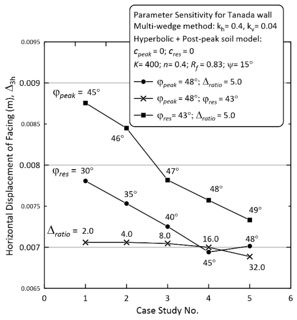
Figure 23 shows the computed Δ3h for variations in K (100–900), n (−0.2–0.6), Rf (0.6–1.0), and ψ (−5–15˚). Among these parameters, K exhibits the strongest influence on Δ3h, consistent with the trends observed in Figure 18. In general, Δ3h decreases nonlinearly as K increases. For K values between 700 and 900, the reduction in Δ3h becomes negligibly small. This behavior reflects the fact that as K increases, the soil stiffness and resistance to seismic loading increase correspondingly, reducing displacement. Once K exceeds a threshold (approximately K = 700 in this case), the soil resistance becomes substantially larger than the seismic demand, and Δ3h remains essentially unchanged. The sensitivity curves for the stress dependency exponent n show that varying n from −0.2 to 0.6 changes Δ3h from 0.014 m to 0.007 m, a total variation of only 0.007 m, suggesting its minor influence on Δ3h. As n increases, the initial stiffness increases more rapidly with depth, resulting in slightly smaller Δ3h. For Rf values ranging from 0.6 to 1.0, Δ3h increases with increasing Rf, and a threshold behavior is observed around Rf = 0.8. From the definition of Rf (ratio of failure strength to asymptotic strength), smaller Rf values correspond to steeper post-failure segments of the stress–displacement curve. Under the medium seismic demand of kh = 0.4, portions of the slip surface may enter the post-failure regime. In such cases, a steeper post-failure segment (smaller Rf) provides greater resistance and yields smaller Δ3h. However, when Rf falls below approximately 0.8, further steepening of the post-failure segment no longer reduces Δ3h, leading to the observed threshold behavior. The variation of ψ from −5° to 15° represents a transition from volume contraction to volume dilation along the failure surface. A displacement field with a negative ψ tends to reduce displacement toward the slope toe with larger displacement concentrated around the crest, whereas a positive ψ promotes displacement toward the toe. The upper-bound value of ψ = 15° is selected based on the experimental observation that the mobilized dilatancy angle at peak state is typically less than 1/2–1/3 of the peak friction angle of sands. Increasing ψ from 0° to 15° produces only a slight increase in Δ3h, while the change from ψ = −5° to 0° produces a relatively larger increase. Nevertheless, the total variation in Δ3h across the entire ψ range is only about 0.005 m. The mechanism underlying this trend is that increasing ψ redistributes displacement more uniformly along the slip surface, reducing crest-concentrated deformation and increasing displacement at the slope toe. These sensitivity results confirm that K is the dominant parameter influencing Δ3h, followed by Rf, ψ, and n. The modest influence of most parameters demonstrates the stability of the seismic resistance curves developed in Section 7 and supports their use in the forensic interpretation presented in the next section.
Figure 23.
Sensitivity of the computed wall displacement to hyperbolic and hodogram parameters.
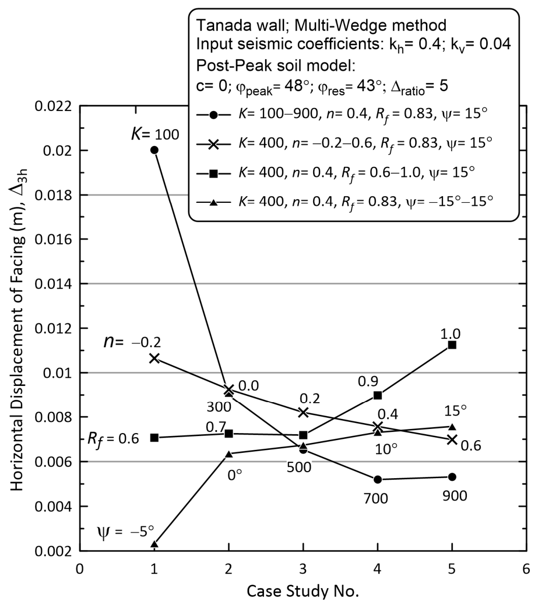
Figure 24 presents the results of the sensitivity investigation on reinforcement-related parameters, including the hyperbolic reinforcement pullout model parameters Kt (initial stiffness number), nt (stress dependency exponent), Rt (failure ratio), Tf (tie-break strength), and φs-r (soil–reinforcement interface friction angle). Among all reinforcement parameters examined, Kt exhibits the most significant influence on Δ3h. As Kt increases, Δ3h decreases noticeably. This trend is analogous to the influence of K on Δ3h observed in Figure 23 for the soil backfill. A larger Kt produces greater reinforcement force at a given pullout displacement, which in turn reduces the lateral facing displacement Δ3h. For the full ranges of nt (−0.2 to 0.6) and Rt (0.6 to 0.9), only slight increases in Δ3h are observed, and the underlying mechanism is similar to that for the soil backfill in Figure 23. The variations in Δ3h induced by changes in nt and Rt remain small, on the order of 0.0002 m. In contrast, varying Kt from 5 to 20, representing a ±100% change from the benchmark value of Kt = 10, produces a larger but still modest variation in Δ3h of approximately 0.003 m. Variations of Tf by approximately ±60% from the benchmark value of Tf = 30 kN/m result in changes in Δ3h of less than 0.001 m. A similarly small influence is observed when the soil–reinforcement interface friction angle φs-r is increased from 10° to 50°. Overall, the sensitivity results show that even with wide-range variations in facing-related and reinforcement-related parameters, their influences on Δ3h are small (on the order of 0.002–0.003 m) compared with those of the soil parameters examined in Figure 23, which shows that the influence of K for a change from K= 250 to K= 600 is on the order of 0.01 m. A qualitative ranking of the influence of the facing and reinforcement parameters can be summarized as Kt > φback > φbase ≈ RFconnect ≈ Tf ≈ φs-r. This hierarchy highlights that uncertainties in facing and reinforcement properties introduce only minimal variations in the final output Δ3h. The robustness of the seismic resistance curves developed in Section 7 is therefore not compromised by reasonable uncertainties in these parameters, reinforcing the conclusion that displacement variability is governed primarily by soil behavior rather than by facing or reinforcement characteristics.
Figure 24.
Sensitivity of the computed wall displacement to reinforcement parameters.
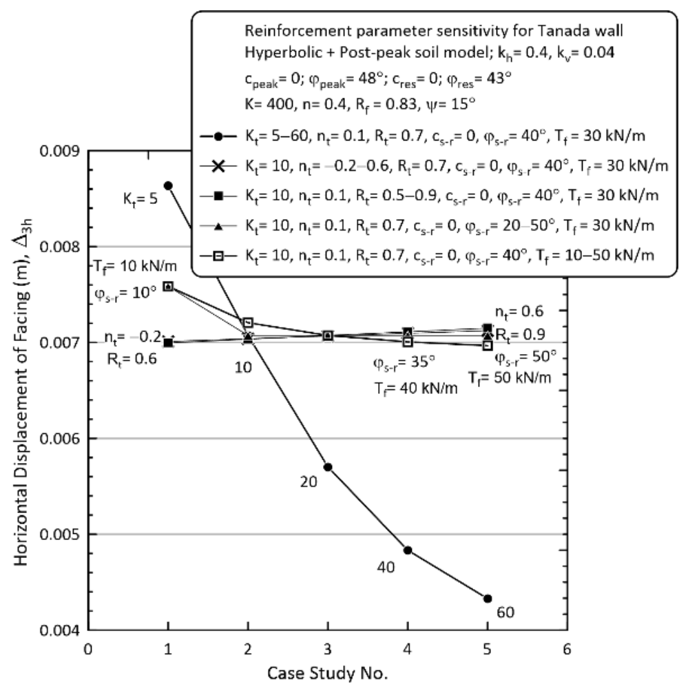
Figure 25 shows the results of the sensitivity investigation on facing-related input parameters, including the friction angle at the facing base (φbase), the facing–backfill interface friction angle (φback), and the connecting strength reduction factor at the reinforcement–facing junction (RFconnect =1: full-strength mobilization at facing–backfill interface). Increasing φbase from 40° to 48° results in a reduction in Δ3h of less than 0.001 m. A similarly small influence is observed when RFconnect is increased from 0.2, representing only 20% of the tie-break strength of the reinforcement, to 1.0, representing full tie-break strength. RFconnect scales the mobilized reinforcement force at the facing connection, but even large changes in this parameter produce only minimal changes in Δ3h. At first glance, φback appears to exert a stronger influence on Δ3h than the other facing-related parameters. This impression arises only because φback is varied over an intentionally broad range (25–45°), representing a 180% change selected to encompass diverse design practices and in situ conditions, including compaction quality near the facing, facing type, and construction sequence. Even across this unusually wide input range, the resulting variation in Δ3h is only about 0.002 m, indicating that the influence of φback on displacement is consistent but modest.
Figure 25.
Sensitivity of the computed wall displacement to the input facing-related parameter.
These results also reinforce the consistency and accuracy of the computational algorithm implemented in SLOPE-ffdm 2.0. The sensitivity study shows that only a small group of primary parameters—specifically the soil stiffness K, the peak friction angle φpeak, and the reinforcement initial pullout stiffness number Kt—exert a dominant and clearly measurable influence on the final displacement Δ3h. These primary parameters are well constrained by the compiled laboratory dataset and therefore carry relatively low uncertainty, while all remaining soil, reinforcement, and facing parameters introduce only minor variations in Δ3h on the order of a few 10−4 m. This hierarchy of influence confirms that the displacement-based seismic resistance curves are robust and that the primary conclusions drawn from the main analysis remain stable and reliable.
9. Discussion
- LEM-based vs. FFDM-based seismic resistance curves:
Figure 26 compares two curves extracted from Figure 17 and Figure 21, representing the LEM-based and FFDM-based seismic resistance curves, respectively. The Fs–kh curve, where Fs > 1.0, provides only an approximate indication of a “safe structure.” Once Fs falls below unity, the limit equilibrium framework offers no quantitative measure of deformation, and performance assessments rely heavily on empirical judgment. In contrast, the displacement-based curves (Δ3h) span three logarithmic cycles (10−3–10−1 m) and respond systematically to increasing levels of input kh. This accurate and consistent seismic displacement output substantiates the engineering judgment on the accessibility of displacement-sensitive structures, such as railways and vital transportational facilities. As an example, [90] provides displacement criteria for facilities that are displacement sensitive and vital to transportation, such as the backfill of a railway bridge abutment. In such applications:
- Δ3h or Δ0 smaller than 10−2 m may be classified as an “Intact” or “Non damaged” condition.
- Δ3h or Δ0 between 10−2 and 10−1 m may be classified as “Lightly damaged,” requiring minor post-earthquake retrofit.
- Δ3h or Δ0 exceeding 2 × 10⁻¹ m may be classified as “Severely damaged,” requiring long-term restoration.
Figure 26.
Example of LEM-based and FFDM-based seismic resistance curves.
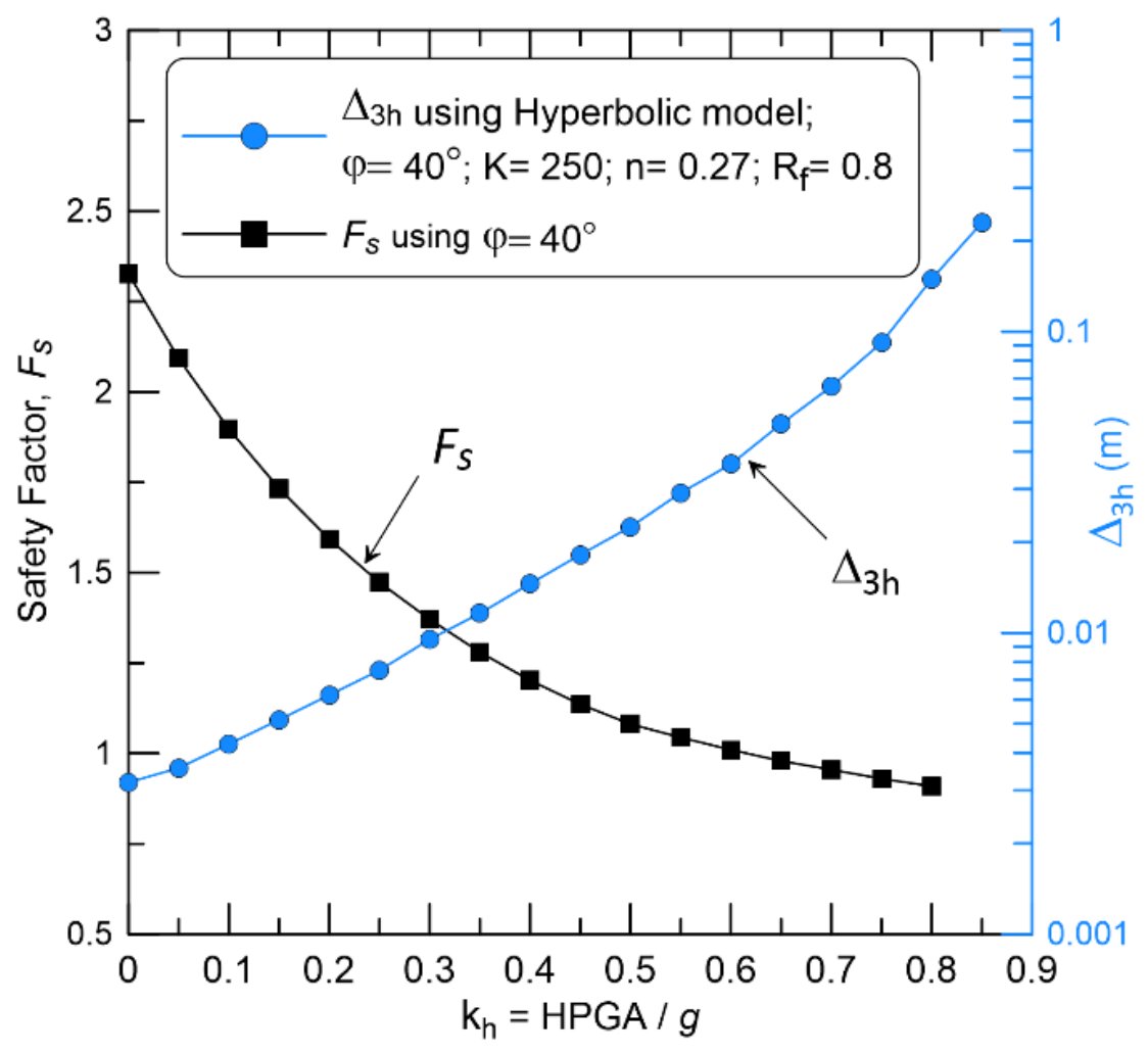
These criteria highlight the engineering advantage of using the displacement-based Δ3h–kh curve rather than the force-based Fs–kh curve. In the context of forensic engineering, the Δ3h–kh curve functions as a true capacity curve, linking seismic demand to deformation response in a manner that the Fs–kh curve cannot achieve.
- 2.
- Essential elements of a successful FFDM-based forensic investigation:
Five elements form the backbone of a reliable FFDM-based forensic investigation. The first element is the development of a soil stress–displacement and reinforcement pullout datasets, as demonstrated in Figure 10, Figure 11, Figure 12, Figure 13 and Figure 14 and Table 4, which provide the empirical foundation for selecting realistic soil and reinforcement parameters. The second element is the LEM analysis for establishing the Fs–φ relationship, as shown in Figure 16, which constrains the operational friction angle consistent with observed stability conditions. The third element is the displacement-based back analysis for determining the hyperbolic parameters K, n, and Rf, as demonstrated in Figure 18, ensuring that the selected parameters reproduce the observed deformation. The fourth element is the parameter sensitivity investigation, as demonstrated in Figure 22, Figure 23, Figure 24 and Figure 25, which evaluates the robustness of the FFDM predictions and identifies the dominant parameters governing displacement. The fifth element is the establishment of displacement-based seismic resistance curves using the best-estimated parameters from the dataset and back analyses. These curves may also possess predictive capability for assessing future behavior of the structure under different seismic scenarios. Although this predictive capability is not demonstrated here because the Tanada wall has already experienced an extreme shaking event (kh ≈ 0.7–0.8), the hypothesis can be verified in the future using well-instrumented and well-documented case histories.
- 3.
- Consistency between back-calculated and measured friction angles and independence of validation:
The median back-calculated internal friction angle of the Tanada wall backfill, φ = 42°, is consistent with the triaxial compression test results on retrieved post-earthquake samples reported in [24], which yielded φtriaxial = 42°. This agreement reflects a well-established pattern in forensic geotechnical engineering rather than an isolated coincidence. Numerous back analyses of slope and embankment failures have shown that the mobilized friction angle inferred from field deformation commonly corresponds to the peak friction angle measured in triaxial compression on undisturbed or representative samples, as demonstrated by the Aberfan waste tip failure [91], the deformation of the Lower San Fernando Dam upstream shell during the 1971 earthquake [92], rainfall-induced failures in Hong Kong saprolites [93], rainfall-triggered colluvial slope failures in Japan [94], and reinforced soil wall failures examined through detailed forensic back analysis [95]. This convergence between mobilized and laboratory friction angles is therefore a characteristic outcome of slope failure mechanics.
It is also important to clarify that the triaxial friction angle for the Tanada backfill was not used as a calibration target in the displacement-based back analysis. The triaxial friction angle was examined only after the back-calculated parameters were obtained and therefore serves as independent validation rather than calibration evidence. The agreement between mobilized ϕ and ϕtriaxial is an outcome of the analysis and indicates that the inferred operational strength lies within a realistic and experimentally supported range. Because the triaxial result was not used to select or adjust the back-calculated parameters, the agreement does not reflect parameter-selection bias and does not constitute circular validation.
- 4.
- Parameter uncertainty and robustness of the back-calculated parameter range:
Parameter uncertainty was evaluated through a systematic sensitivity investigation in which all input parameters were varied over wide physically meaningful ranges. The results demonstrate a clear hierarchy of influence: only ϕpeak, the stiffness number of soil K, and the initial pullout stiffness number of reinforcement, Kt, exert dominant control on the predicted toe displacement Δ3h, whereas all remaining soil, reinforcement, and facing parameters produce negligible variations. This hierarchy indicates that the back-calculated parameters represent operational values governed primarily by the observed displacement rather than arbitrary selections within broad material ranges. Additional quantification using the coefficient of variation reported in [22] shows that a representative Coefficient of Variation (COV )of 7% for ϕpeak, K, and Kt leads to variations in Δ3h of approximately ±1.2 mm, ±1.5 mm, and ±0.8 mm, respectively, all of which remain well within the observed toe displacement of 100 mm. Because the influence of all other parameters on Δ3h is minimal, their uncertainties are practically insignificant. The resulting parameter range is therefore physically constrained, empirically supported, and robust with respect to both laboratory variability and field measurement uncertainty.
These four aspects collectively demonstrate that the FFDM, when supported by a soil dataset, LEM-based strength constraints, displacement-based back analysis, and systematic sensitivity evaluation, provides a physically grounded and performance-oriented framework for forensic geotechnical engineering. The resulting displacement-based seismic resistance curves offer a robust foundation for forensic interpretation and for future applications to well-documented case histories.
10. Conclusions
This study presents a performance-based forensic investigation aimed at identifying representative soil parameters and establishing displacement-based seismic resistance curves for the Tanada wall, a geosynthetic reinforced soil wall with a full-height rigid panel facing. By integrating laboratory evidence, limit equilibrium constraints, displacement-based back analysis, and systematic parameter sensitivity evaluation, the study reconstructs the seismic behavior of the structure during the 1995 Hyogoken-Nambu earthquake in Japan and provides a physically grounded basis for forensic interpretation, with potential applicability to forward predictions for similar reinforced soil systems. The major conclusions are summarized as follows.
- A compiled soil stress–displacement dataset provides the empirical foundation for FFDM-based forensic analysis. The dataset developed in this study establishes relationships between internal friction angle and the hyperbolic parameters K, n, and Rf. These relationships supply physically meaningful bounds for selecting representative soil parameters and ensure that the FFDM analysis is anchored in experimentally supported soil behavior.
- Limit-equilibrium-based back analysis provides first approximate bounds of the operational friction angle, yielding values such as φ = 39.5° under kh = 0.4 that remain essential for subsequent displacement-based evaluation. Using Fs–φ curves, a plausible range of φ = 40–44° is identified for the Tanada wall. However, the displacement-based back analysis and the seismic resistance curves demonstrate that HPGA = 0.42 g is unlikely to have occurred at the site. The observed displacement Δ3h = 0.1 m cannot be produced by kh = 0.4, indicating that the actual shaking intensity was significantly higher. This finding highlights the limitation of relying solely on LEM-based stability and underscores the necessity of displacement-based tools in forensic reconstruction.
- Displacement-based back analysis identifies representative hyperbolic parameters and reconstructs the Δ3h–kh seismic resistance curve, which expresses the deformation response under varying seismic intensities. Matching the observed base displacement yields K = 200–300 and Rf ≈ 0.8 as the most plausible in situ parameters. These values align closely with the bounds inferred from the compiled dataset (K = 250–600 for φ = 40–44°), confirming consistency between laboratory evidence and field-scale behavior. The agreement between the back-calculated friction angle (φ = 42°) and the triaxial test result from the retrieved samples (φtriaxial = 42°) serves as independent validation because the triaxial result was not used as a calibration target. This consistency supports the use of φ = 42° as the operational strength of the backfill.
- Displacement-based seismic resistance curves provide a robust and physically meaningful performance measure. Using the back-calculated and dataset-supported soil parameters, Δ3h–kh curves are established for both hyperbolic and composite (hyperbolic + post-peak) soil models. These curves show that the Tanada wall exhibits strong seismic resistance up to kh ≈ 0.7–0.75, with Δ3h values on the order of 3–23 × 10−2 m. The curves span three logarithmic cycles of displacement and respond smoothly to an increasing seismic inertial coefficient (kh), demonstrating the physical realism and numerical stability of the FFDM algorithm. These curves again confirm that the observed displacement cannot be generated by kh = 0.4, reinforcing the conclusion obtained in the post-earthquake site investigation and the displacement-based back analysis that the actual shaking intensity was substantially higher, at kh ≈ 0.7.
- Parameter sensitivity investigations confirm the robustness and reliability of the seismic resistance curves. Sensitivity analyses show that only a small subset of parameters—specifically the soil stiffness number K, the peak friction angle φpeak, and the initial pullout stiffness number Kt—exert a dominant influence, producing variations of approximately ±0.8–1.5 × 10⁻³ m in the final displacement Δ3h. These primary parameters are well constrained by the compiled laboratory dataset and therefore carry relatively low uncertainty, while all remaining soil, reinforcement, and facing parameters introduce only minor variations in Δ3h on the order of a few 10−4 m. This hierarchy of influence demonstrates that the displacement-based seismic resistance curves are stable and largely insensitive to reasonable uncertainties in secondary parameters, thereby reinforcing the reliability of the forensic interpretation.
Overall, the study shows that the FFDM—when supported by a compiled soil stress–displacement dataset, LEM-based strength constraints, displacement-based back analysis, and systematic sensitivity evaluation—provides a rigorous and physically grounded framework for performance-based forensic geotechnical engineering. Because the primary parameters governing Δ3h are laboratory-supported and exhibit limited uncertainty, the resulting displacement-based seismic resistance curves possess high reliability. These curves indicate that the Tanada wall likely experienced shaking intensities on the order of 0.7–0.8 g, far exceeding a possible shaking intensity of HPGA = 0.42 g recorded at a seismograph located approximately 2 km from the Tanada wall site. The framework also has potential predictive capability for future seismic performance assessments, and verification using well-instrumented case histories represents an important direction for future research.
Funding
This research received no external funding.
Institutional Review Board Statement
Not applicable.
Informed Consent Statement
Not applicable.
Data Availability Statement
The raw data supporting the conclusions of this article will be made available by the authors on request.
Acknowledgments
The author appreciates the valuable suggestions provided by H.-Y. Shieh, I. Hamadiyah, A. Tang, and Z. Lin of ACE Geosynthetic Inc. in Taichung, Taiwan, particularly their assistance in identifying software bugs and improving user-friendly functions of SLOPE-ffdm 2.0. The valuable pre- and post-earthquake photos of the Tanada wall provided by M. Tateyama of Japan Transportation Consultants, Inc. are also highly appreciated.
Conflicts of Interest
The authors declare no conflict of interest.
References
- Alonso, E.E.; Pinyol, N.; Fernández, P. Caisson Failure Induced by Wave Action. In Forensic Geotechnical Engineering; Springer: New Delhi, India, 2016; pp. 63–82. [Google Scholar]
- Leonards, G.A. Investigation of failures. J. Geotech. Eng. Div. ASCE 1982, 108, 187–246. [Google Scholar] [CrossRef] [Scilit]
- Huang, C.-C. Developing a new slice method for slope displacement analyses. Eng. Geol. 2013, 157, 39–47. [Google Scholar] [CrossRef] [Scilit]
- Huang, C.-C. Force equilibrium-based finite displacement analyses for reinforced slopes: Formulation and verification. Geotext. Geomembr. 2014, 42, 394–404. [Google Scholar] [CrossRef] [Scilit]
- Vidal, H. Peau pour ouvrages en terre armée (Reinforced Earth). Swiss Patent CH528639A, 1969. [Google Scholar]
- Vidal, H. Reinforced Earth. Ann. Inst. Tech. Batim. Trav. Publics 1969, 30, 888–938. [Google Scholar]
- Schlosser, F. Behaviour of Reinforced Earth Structures. In Proceedings of the Symposium on Reinforced Earth, Pairs; Institution of Civil Engineers: London, UK, 1978. [Google Scholar]
- Reinforced Earth Company (RECo). First Reinforced Earth Wall Built in France; RECo Technical Report; Reinforced Earth Company: Paris, France, 1965. [Google Scholar]
- Reinforced Earth Company (RECo). Reinforced Earth: 50 Years of Innovation; RECo Publication; Reinforced Earth Company: Reston, VA, USA, 2024. [Google Scholar]
- Freitag, N. Reinforced Earth and Its Heritage. In Proceedings of the CFMS Coulomb Tribute Conference, Paris, France, 25–26 September 2023. [Google Scholar]
- Murata, O.; Tateyama, M.; Tatsuoka, F. Shaking Table Tests on a Large Geosynthetic Reinforced Soil Retaining Wall Model. In Recent Case Histories of Permanent GRS Walls; Leshchinsky, D., Tatsuoka, F., Eds.; Balkema: Rotterdam, The Netherlands, 1994; pp. 259–264. [Google Scholar]
- Tatsuoka, F.; Tateyama, M.; Uchimura, T.; Koseki, J. Geosynthetic Reinforced Soil Retaining Walls as Important Permanent Structures. Geosynth. Int. 1997, 4, 81–136. [Google Scholar] [CrossRef] [Scilit]
- Tatsuoka, F.; Tateyama, M.; Koseki, J. Performance of soil retaining walls for railway embankments. Jpn. Geotech. Soc. 1996, 36, 311–324. Available online: https://www.sciencedirect.com/science/article/pii/S0038080620330146/pdf?md5=dfab003d3f12d998e2950b7d0a073bae&pid=1-s2.0-S0038080620330146-main.pdf (accessed on 8 August 2026). [CrossRef] [Scilit] [PubMed]
- Watanabe, K.; Munaf, Y.; Koseki, J.; Tateyama, M.; Kojima, K. Behaviors of Several Types of Model Retaining Walls Subjected to Irregular Excitation. Soils Found. 2003, 43, 13–27. [Google Scholar] [CrossRef] [Scilit] [PubMed]
- Hirakawa, D.; Nojiri, M.; Aizawa, H.; Tatsuoka, F.; Sumiyoshi, T.; Uchimura, T. Behaviour of GRS Retaining Wall Subjected to Forced Cyclic Horizontal Displacement. In Proceedings of the 8th International Conference on Geosynthetics, Yokohama; Millpress: Rotterdam, The Netherlands, 2006; pp. 1075–1078. [Google Scholar]
- Japan Railway Technical Research Institute (JRTRI). Design Guideline for Railway Structures-Soil Structures; Maruzen: Tokyo, Japan, 1992. (In Japanese) [Google Scholar]
- Huang, C.-C.; Chou, L.H.; Tatsuoka, F. Seismic displacements of geosynthetic-reinforced soil modular block walls. Geosynth. Int. 2003, 10, 2–23. [Google Scholar] [CrossRef] [Scilit]
- SLOPE-ffdm 2.0: Computer Programs for Slope Stability and Displacement Analyses Using Force-Equilibrium-Based Finite Displacement Method (FFDM). 2025. Available online: https://slope.it.com/ (accessed on 8 August 2026).
- Sivakumar Babu, G.L.; Singh, V.P. Back Analyses in Geotechnical Engineering. In Forensic Geotechnical Engineering; Springer: New Delhi, India, 2016; pp. 125–146. [Google Scholar]
- Popescu, M.E.; Schaefer, V.R. Back Analysis of Slope Failures to Design Landslide Stabilizing Piles. In Forensic Geotechnical Engineering; Springer: New Delhi, India, 2016; pp. 147–166. [Google Scholar]
- Skempton, A.W. Long term stability of clay slopes. Géotechnique 1964, 14, 75–101. [Google Scholar] [CrossRef] [Scilit]
- Duncan, J.M.; Wright, S.G. Soil Strength and Slope Stability; John Wiley & Sons: Hoboken, NJ, USA, 2005. [Google Scholar]
- Mandal, J.N.; Narwal, R.P.; Gupte, S.S. Back analysis of failed slopes: A case study. Int. J. Eng. Res. Technol. 2017, 6, 1–6. [Google Scholar]
- Tateyama, M. Back analyses of damaged retaining structures for railway by Hyogoken-Nambu earthquake. RTRI Rep. 1996, 10, 11–16. (In Japanese) [Google Scholar]
- Tatsuoka, F.; Koseki, J.; Tateyama, M.; Munaf, Y.; Horii, K. Seismic stability against high seismic loads of geosynthetic-reinforced soil retaining structures. In Proceedings of the 6th International Conference on Geosynthetics, Atlanta, USA; Industrial Fabrics Association International: St. Paul, MN, USA, 1998; pp. 103–142. [Google Scholar]
- Elias, V.; Christopher, B.R.; Berg, R.R. Mechanically Stabilized Earth Walls and Reinforced Soil Slopes: Design and Construction Guidelines; FHWA NHI 00 043; Federal Highway Administration: Washington, DC, USA, 2001.
- Berg, R.R.; Christopher, B.R.; Samtani, N.C. Design and Construction of Mechanically Stabilized Earth Walls and Reinforced Soil Slopes; FHWA NHI 10 024; Federal Highway Administration: Washington, DC, USA, 2009.
- Taylor, T.P.; Collin, J.G.; Boyle, S.; Fishman, K.; Han, J. Design and Construction of Mechanically Stabilized Earth (MSE) Walls; FHWA HIF 24 002; Federal Highway Administration: Washington, DC, USA, 2023.
- National Concrete Masonry Association. Deisgn Manual for Segmental Retaining Walls, 3rd ed.; National Concrete Masonry Association: Herndon, VA, USA, 2012. [Google Scholar]
- Newmark, N.M. Effects of earthquakes on dams and embankments. Geotechnique 1965, 15, 139–160. [Google Scholar] [CrossRef] [Scilit]
- Richard, R.M.; Elms, D.G. Seismic behavior of gravity retaining walls. J. Geotech. Eng. Div. ASCE 1979, 105, 449–464. [Google Scholar] [CrossRef] [Scilit]
- Whitman, R.V.; Liao, S.S.C. Seismic design of gravity retaining walls. In Proceedings of the ASCE Geotechnical Engineering Division Specialty Conference on Earth Retaining Structures, Ithaca, NY; American Society of Civil Engineers: New York, NY, USA, 1987; pp. 817–842. [Google Scholar]
- Cai, Z.; Bathurst, R.J. Deterministic sliding block methods for estimating seismic displacements of earth structures. Soil Dyn. Earthq. Eng. 1996, 15, 255–268. [Google Scholar] [CrossRef] [Scilit]
- Silva, F.; Lambe, T.W.; Marr, W.A.; Bachus, R.C. Probability of failure for geotechnical structures. In Proceedings of the GeoCongress 2008: Geotechnics of Waste Management and Remediation; ASCE: Reston, VA, USA, 2008; pp. 1–10. [Google Scholar]
- Day, R.W. Forensic Geotechnical and Foundation Engineering, 2nd ed.; McGraw Hill Education: New York, NY, USA, 2016. [Google Scholar]
- Srivastava, A.; Sharma, K.; Jakka, R. Forensic investigation of geotechnical failures: Lessons from recent case histories. Innov. Infrastruct. Solut. 2025, 10, 45–62. [Google Scholar]
- Cassidy, M.J.; Randolph, M.F.; Quinteros, R. A probabilistic approach to assessing the stability of submarine slopes. Can. Geotech. J. 2008, 45, 1252–1265. [Google Scholar]
- Lacasse, S.; Nadim, F.; Hoeg, K. Risk assessment and mitigation in geotechnical engineering. In Proceedings of the 18th International Conference on Soil Mechanics and Geotechnical Engineering; Comité Français de Mécanique des Sols: Paris, France, 2013; pp. 269–302. [Google Scholar]
- Phoon, K.K.; Ching, J.; Juang, C.H. Characterization of geotechnical variability and its impact on design. Georisk Assess. Manag. Risk Eng. Syst. Geohazards 2016, 10, 1–27. [Google Scholar]
- Huang, C.C. The seismic response of two geotechnically similar GRS-MB walls during the Chi-Chi earthquake: Insights from the finite displacement method. Geotechnics 2026, 6, 39. [Google Scholar] [CrossRef] [Scilit]
- Kim, S.J.; Kurama, Y.C. An alternative pushover analysis procedure to estimate seismic displacement demands. Eng. Struct. 2008, 30, 3793–3807. [Google Scholar] [CrossRef] [Scilit]
- Yip, W.K.; Li, B.; Fardis, M.N. Improved pushover procedures for performance based seismic assessment. Earthq. Eng. Struct. Dyn. 2017, 46, 567–585. [Google Scholar] [CrossRef] [Scilit]
- Gunes, B. Evaluation of nonlinear static procedures for seismic performance assessment of structures. Soil Dyn. Earthq. Eng. 2020, 130, 105984. [Google Scholar]
- Ito, T.; Matsui, T. Methods to estimate lateral force acting on stabilizing piles. Soils Found. 1975, 15, 43–59. [Google Scholar] [CrossRef] [Scilit] [PubMed]
- Huang, C.-C.; Wang, W.-C. Seismic displacement of a geosynthetic-reinforced wall in the 1995 Hyogo-Ken Nambu earthquake. Soils Found. 2005, 45, 1–10. [Google Scholar] [CrossRef] [Scilit] [PubMed][Green Version]
- Bolton, M.D. The strength and dilatancy of sands. Géotechnique 1986, 36, 65–78. [Google Scholar] [CrossRef] [Scilit]
- Tatsuoka, F.; Molenkamp, F.; Torii, T.; Hino, T. Behavior of plane strain compression tests on sand and its application to constitutive modeling. Soils Found. 1986, 26, 65–84. [Google Scholar]
- Tatsuoka, F.; Ishihara, K. Drained deformation of sand under cyclic stresses reversing direction. Soils Found. 1974, 14, 51–65. [Google Scholar] [CrossRef] [Scilit] [PubMed]
- Lade, P.V.; Lee, K.L. Engineering properties of soils based on drained tests. J. Geotech. Eng. Div. ASCE 1976, 102, 123–136. [Google Scholar]
- Lade, P.V. Elasto plastic stress strain theory for cohesionless soil with curved yield surfaces. Int. J. Solids Struct. 1977, 13, 1019–1035. [Google Scholar] [CrossRef] [Scilit]
- Been, K.; Jefferies, M.G. A state parameter for sands. Géotechnique 1985, 35, 99–112. [Google Scholar] [CrossRef] [Scilit]
- Verdugo, R.; Ishihara, K. The steady state of sandy soils. Soils Found. 1996, 36, 81–91. [Google Scholar] [CrossRef] [Scilit] [PubMed]
- Lo, C.-L.; Huang, C.-C. Displacement analyses for a natural slope considering post-peak strength of soils. GeoHazards 2021, 2, 41–62. [Google Scholar] [CrossRef] [Scilit]
- Chiang, Y.-J. Analyses for Rainfall-Induced Slope Displacements Taking into Account Various Displacement Fields and Failure Criteria. Master Thesis, National Cheng Kung University, Tainan, Taiwan, 2017. [Google Scholar]
- Chu, B.-L.; Huang, C.-R.; Jeng, S.-Y. Study on terrace sedimentary and Tou-ka-san gravelly strata using in-situ direct shear tests. In Proceedings of the 3rd National Geotechnical Conference, Taichung City, Taiwan; Geotechnical Engineering Research and Development Foundation: Taipei, Taiwan, 1989; pp. 695–706. [Google Scholar]
- Qiu, J.-Y.; Tatsuoka, F.; Uchimura, T. Constant Pressure and Constant Volume Direct Shear Tests on Reinforced Sand. Soils Found. 2000, 40, 1–17. [Google Scholar] [CrossRef] [Scilit] [PubMed][Green Version]
- Davoudi, M.H. Influence of willow root density on shear resistance parameters in fine grain soils using in situ direct shear tests. Res. J. Environ. 2011, 5, 157–170. [Google Scholar] [CrossRef] [Scilit]
- Wu, K.-W. Applying Results of True Direct Shear Tests to the Stability Analysis for Integrated Road-Dyke Structures. Master’s Thesis, Feng-Chia University, Taichung City, Taiwan, 2011. (In Chinese) [Google Scholar]
- Hsu, H.-Y. Modeling on the Behavior of Soils Subjected to Cyclic Direct Shear. Master’s Thesis, National Cheng Kung University, Tainan, Taiwan, 2017. (In Chinese) [Google Scholar]
- Ziaie Moayed, R.; Alibolandi, M.; Alizadeh, A. Specimen size effects on direct shear test of silty sands. Int. J. Geotech. Eng. 2017, 11, 198–205. [Google Scholar] [CrossRef] [Scilit]
- Wu, P.-K.; Matsushima, K.; Tatsuoka, F. Effects of specimen size and some other factors on the strength and deformation of granular soil in direct shear tests. Geotech. Test. J. 2008, 31, 45–64. [Google Scholar] [CrossRef] [Scilit]
- CNS 11778-1986-12; Method of Test for Direct Shear of Soils. CNS Catalog 2026. Category no. A3253. Bureau of Standards, Metrology and Inspection, Ministry of Economic Affairs, ROC: Taipei, Taiwan.
- Kondner, R.L. Hyperbolic stress–strain response: Cohesive soils. J. Soil Mech. Found. Div. 1963, 89, 115–143. [Google Scholar] [CrossRef] [Scilit]
- Duncan, J.M.; Chang, C.-Y. Nonlinear analysis of stress and strain in soils. J. Soil Mech. Found. Div. ASCE 1970, 96, 1629–1653. [Google Scholar] [CrossRef] [Scilit]
- Wong, K.S.; Duncan, J.M. Hyperbolic Stress–Strain Parameters for Non-Linear Finite Element Analyses of Stresses and Movements in Soil Masses; Report No. UCB/GT/74-01; Department of Civil Engineering, University of California: Berkeley, CA, USA, 1974. [Google Scholar]
- Duncan, J.M.; Byrne, P.; Wong, K.S.; Mabry, P. Strength, Stress–Strain and Bulk Modulus Parameters for Finite Element Analyses of Stresses and Movements in Soil Masses; Report No. UCB/GT/80 01; University of California: Berkeley, CA, USA, 1980. [Google Scholar]
- Tatsuoka, F.; Sakamoto, M.; Kawamura, T.; Fukushima, S. Strength and deformation characteristics of sand in plane strain compression at extremely low pressure. Soils Found. 1986, 26, 65–85. [Google Scholar] [CrossRef] [Scilit]
- Lupini, J.F.; Skinner, A.E.; Vaughan, P.R. The drained residual strength of cohesive soils. Géotechnique 1981, 31, 181–213. [Google Scholar] [CrossRef] [Scilit]
- Skempton, A.W. Residual strength of clays in landslides, folded strata and the laboratory. Géotechnique 1985, 35, 3–18. [Google Scholar] [CrossRef] [Scilit]
- Mesri, G.; Cepeda Diaz, A.F. Residual shear strength of clays and shales. Géotechnique 1986, 36, 269–274. [Google Scholar] [CrossRef] [Scilit]
- Stark, T.D.; Eid, H.T. Drained residual strength of cohesive soils. J. Geotech. Eng. ASCE 1994, 120, 856–871. [Google Scholar] [CrossRef] [Scilit]
- Tika, T.E.; Hutchinson, J.N. Ring shear tests on soil from the Vaiont landslide slip surface. Géotechnique 1999, 49, 59–74. [Google Scholar] [CrossRef] [Scilit]
- Jewell, R.A. Reinforced soil walls: Analysis and performance. Proc. Inst. Civ. Eng. 1990, 89, 317–342. [Google Scholar]
- Palmeira, E.M.; Milligan, G.W.E. Scale and other factors affecting the results of pullout tests of grids buried in sand. Géotechnique 1989, 39, 511–524. [Google Scholar] [CrossRef] [Scilit]
- Lopes, M.L.; Ladeira, M. Influence of compaction on the pullout resistance of geogrids embedded in a residual soil. Geosynth. Int. 1996, 3, 451–474. [Google Scholar]
- Palmeira, E.M. Bearing force mobilization in pullout tests on geosynthetics. Geotext. Geomembr. 2004, 22, 279–296. [Google Scholar]
- Moraci, N.; Recalcati, P. Pullout resistance of geogrids embedded in a compacted granular soil. Geotext. Geomembr. 2006, 24, 220–236. [Google Scholar] [CrossRef] [Scilit]
- Vieira, C.S.; Lopes, M.L.; Caldeira, L.M. Pullout behaviour of geogrids embedded in different backfill soils. Geotext. Geomembr. 2013, 37, 1–16. [Google Scholar]
- Sugimoto, M.; Alagiyawanna, A.M.N. Pullout behavior of geogrid by test and numerical analysis. J. Geotech. Geoenviron. Eng. ASCE 2003, 129, 361–371. [Google Scholar] [CrossRef] [Scilit]
- Sieira, A.C.C.F.; Geoscovich, D.M.S.; Sayao, A.S.F.J. Displacement and load transfer mechanisms of geogrids under pullout condition. Geotext. Geomembr. 2009, 27, 241–253. [Google Scholar] [CrossRef] [Scilit]
- Moraci, N.; Gioffrè, D.; Mandaglio, M.C. Experimental and theoretical investigation on geogrid pullout behavior under different normal stresses. Geotext. Geomembr. 2014, 42, 461–472. [Google Scholar]
- Tajabadipour, M.; Lajevardi, S.H. Laboratory large-scale pullout investigation of a new reinforcement of composite geosynthetic strip. J. Rock. Mech. Geotech. Eng. 2021, 13, 1147–1159. [Google Scholar] [CrossRef] [Scilit]
- Ismail, M.K.A.; Joohari, M.I.; Habulat, A.; Azizan, F.A. Pull-out resistance of sand-geosynthetics reinforcement. Int. J. Integr. Eng. 2021, 13, 87–93. [Google Scholar] [CrossRef] [Scilit]
- Park, J.; Hong, G. Effective length prediction and pullout design of geosynthetic strips based on pullout resistance. Materials 2021, 14, 6151. [Google Scholar] [CrossRef] [Scilit] [PubMed]
- Vieira, C.; Pereira, P.M. Influence of the geosynthetic type and compaction conditions on the pullout behaviour of geosynthetics embedded in recycled construction and demolition materials. Sustainability 2022, 14, 1207. [Google Scholar] [CrossRef] [Scilit]
- Huang, C.-C.; Wang, Z.-H. Installation damage of geogrids: Influence of load intensity. Geosynth. Int. 2007, 14, 65–75. [Google Scholar] [CrossRef] [Scilit]
- Bathurst, R.J.; Allen, T.M.; Walters, D.L. Long term strength and reduction factors for geosynthetic reinforcement. Geotext. Geomembr. 2011, 29, 323–334. [Google Scholar]
- Koerner, R.M. Designing with Geosynthetics, 6th ed.; Xlibris: Bloomington, IN, USA, 2012. [Google Scholar]
- Allen, T.M.; Bathurst, R.J. Observed long-term performance of geosynthetic walls and implications for design. Geosynth. Int. 2002, 9, 567–606. [Google Scholar] [CrossRef] [Scilit]
- Japan Railway Technical Research Institute. Guidelines for the Design of Railway Structures: Seismic Design; Chapter 14: Embankment; Maruzen: Tokyo, Japan, 1999; pp. 317–329. [Google Scholar]
- Bishop, A.W. The stability of tips and spoil heaps. Géotechnique 1973, 23, 267–302. [Google Scholar]
- Seed, H.B.; Lee, K.L. Seismic stability of earth dams. Proc. ASCE Spec. Conf. Earthq. Eng. Soil Dyn. 1976, 2, 215–232. [Google Scholar]
- Geotechnical Engineering Office (GEO). Back Analysis of Slope Failures in Hong Kong; GEO Report No. 42; Hong Kong Government: Hong Kong, 1988.
- Takahashi, A.; Nakata, Y.; Fukuoka, H. Back analysis of rainfall induced slope failures in colluvial soils. In Proceedings of the Japan Landslide Society Annual Meeting; Japan Landslide Society: Tokyo, Japan, 1992. [Google Scholar]
- Bathurst, R.J.; Miyata, Y. Forensic analysis of reinforced soil wall failures. Transp. Infrastruct. Geotechnol. 2015, 2, 3–24. [Google Scholar]
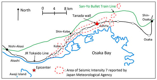
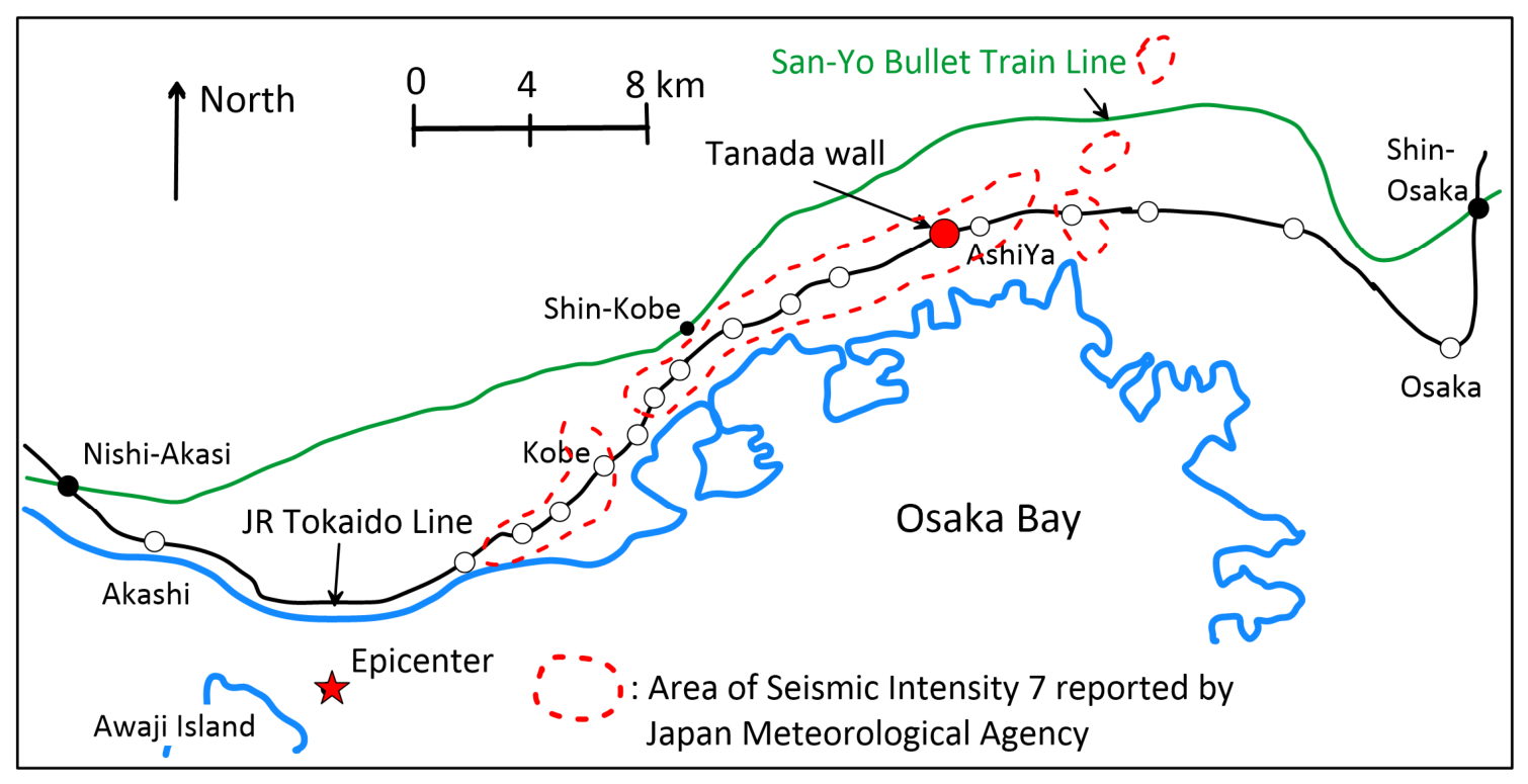
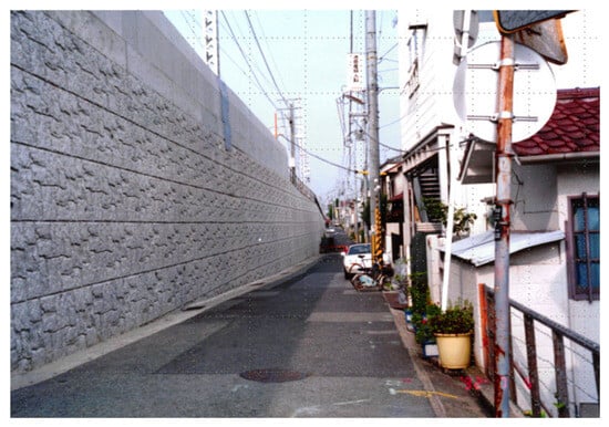
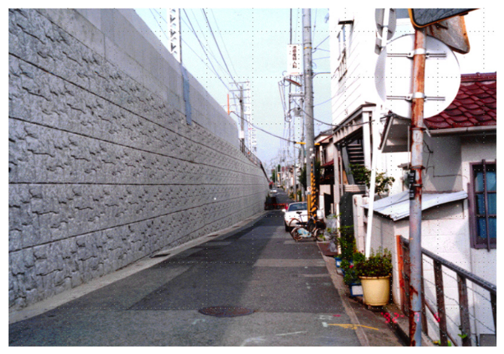
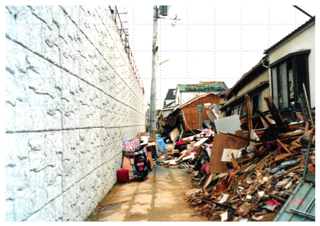
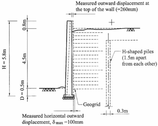
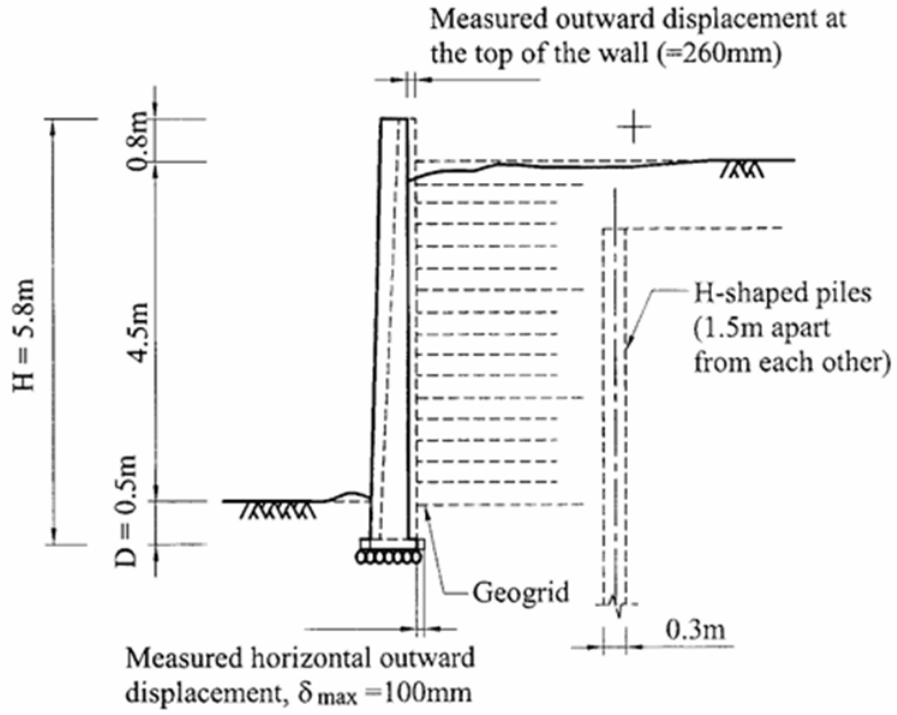
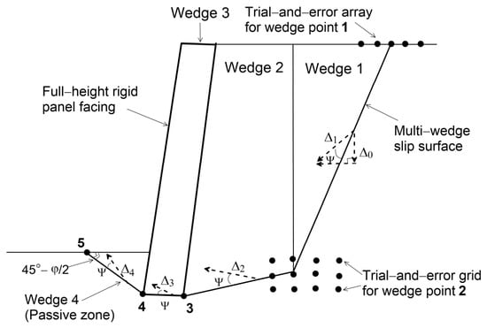
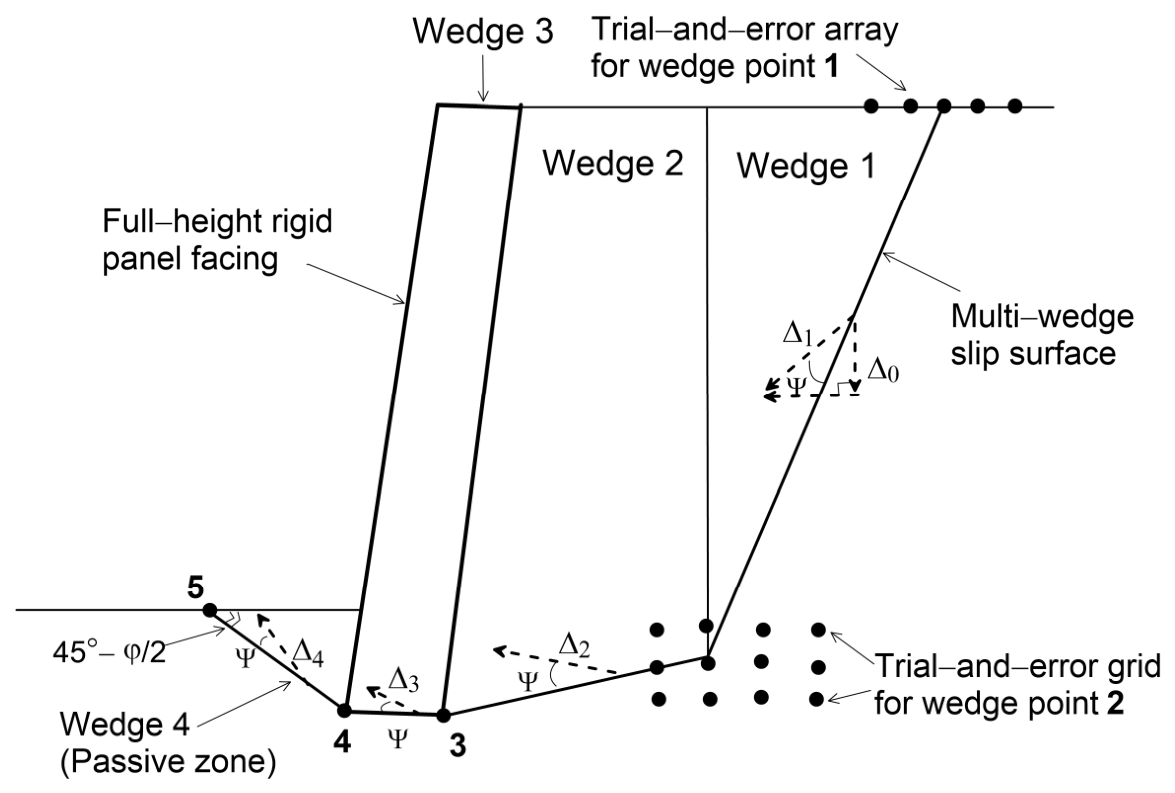
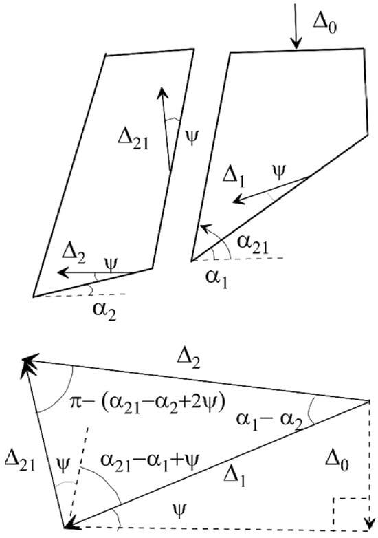
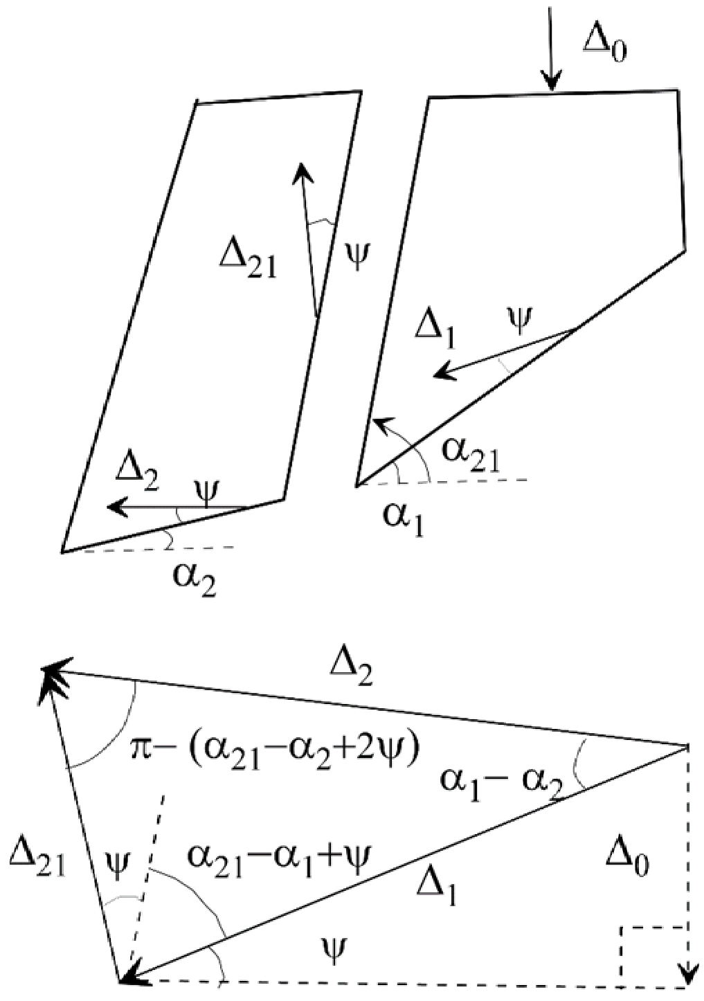
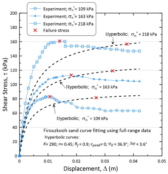
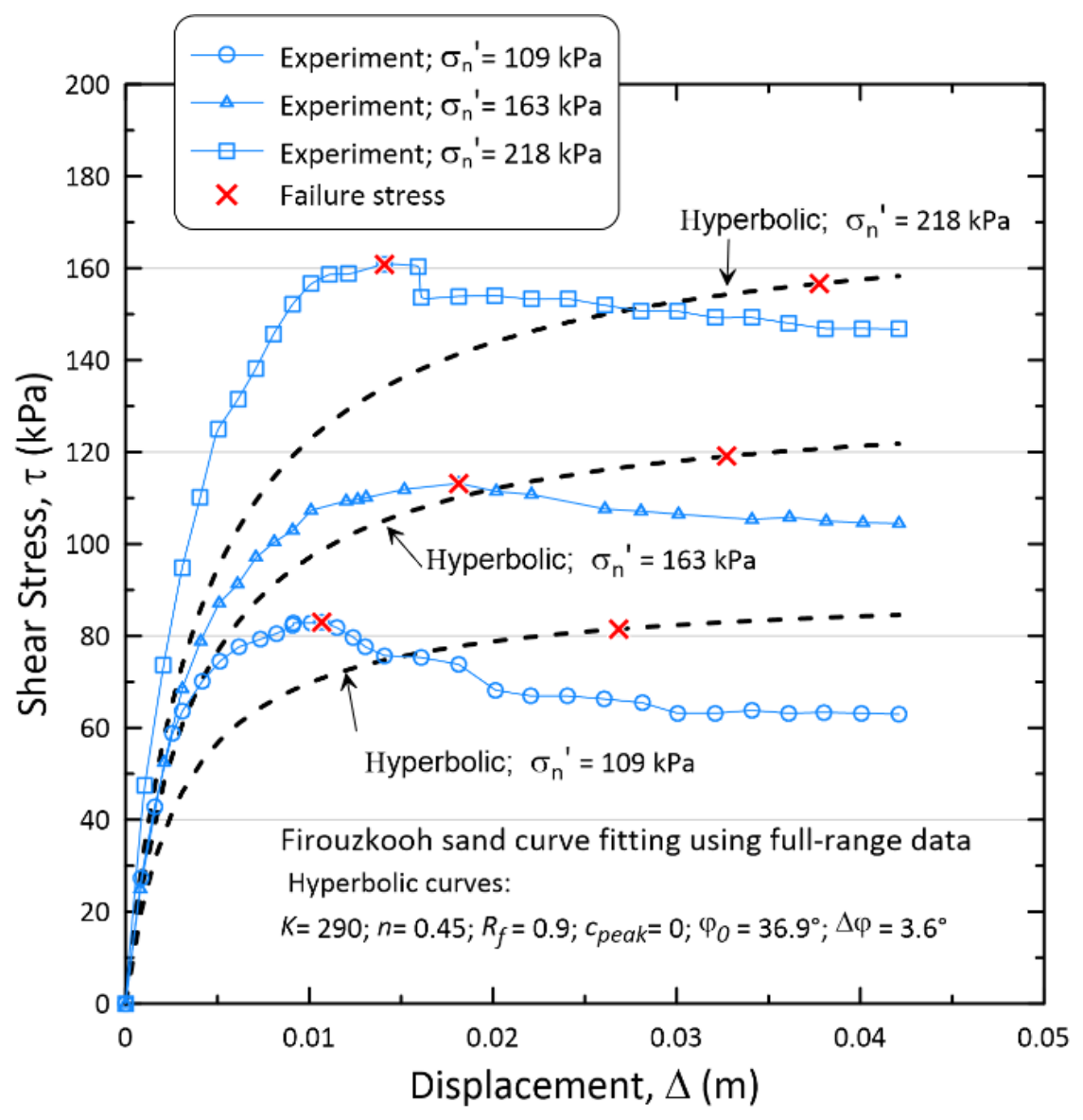
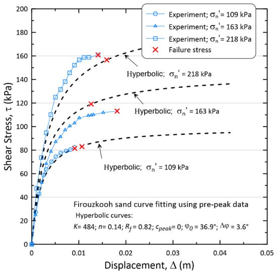
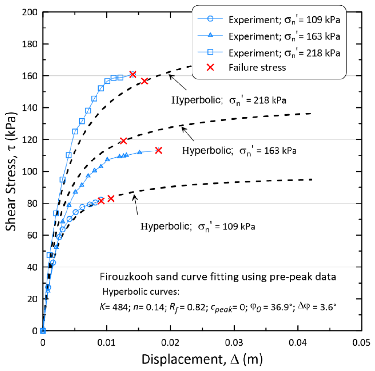
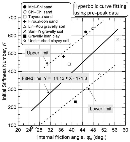
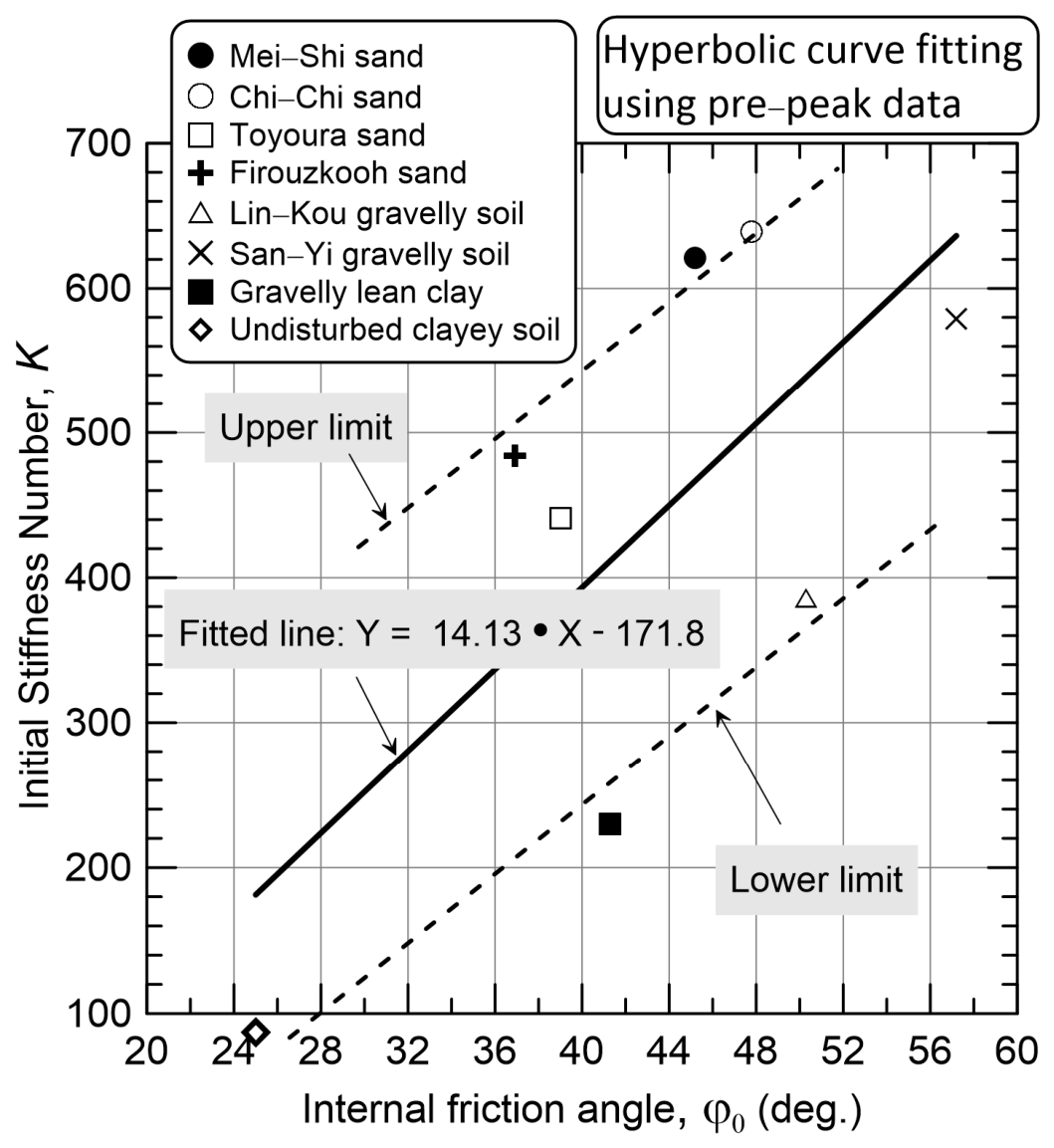
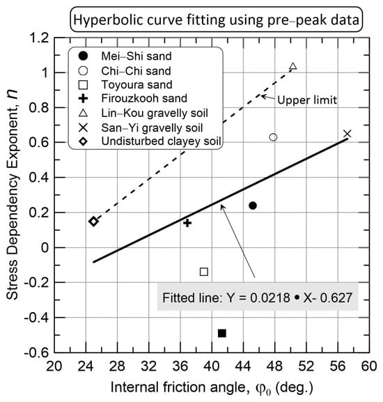
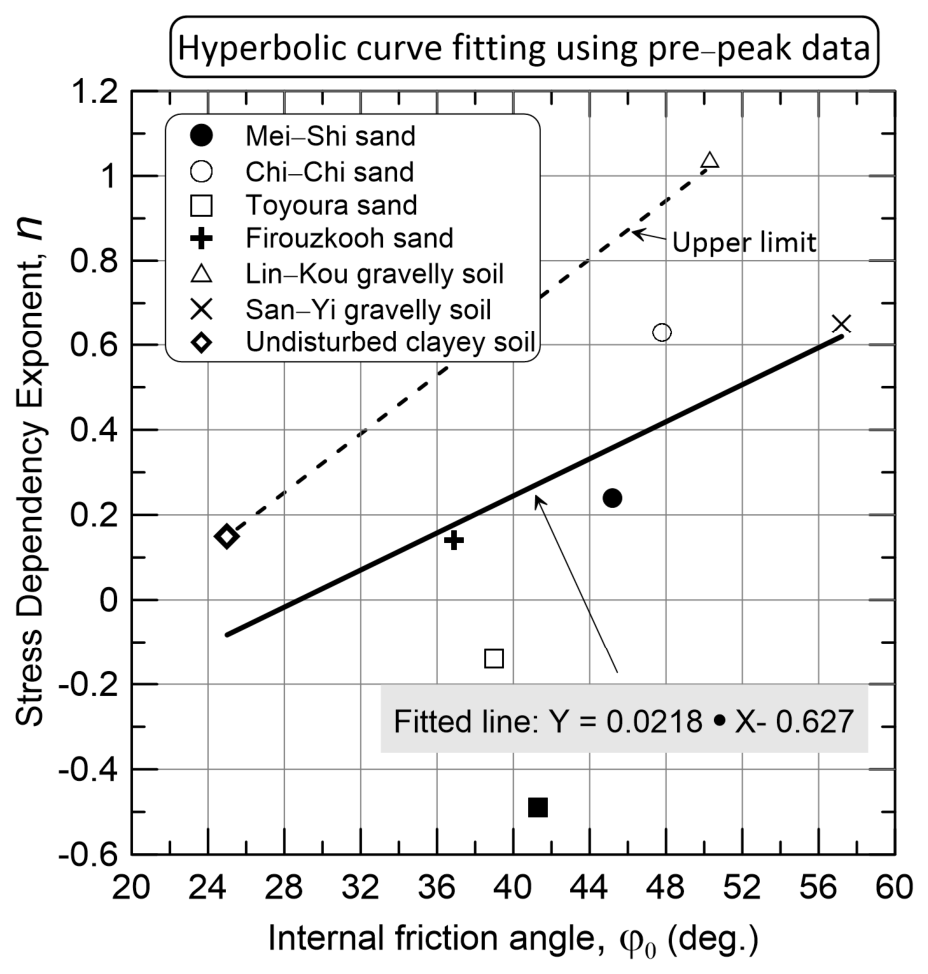
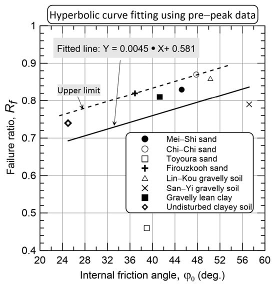
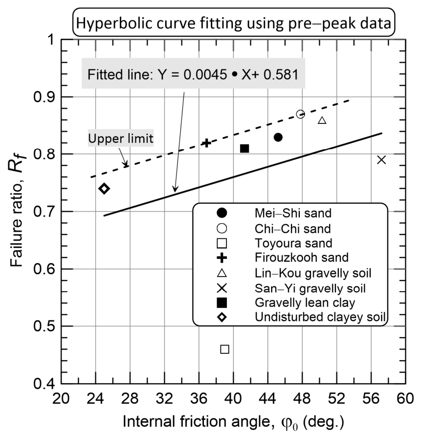
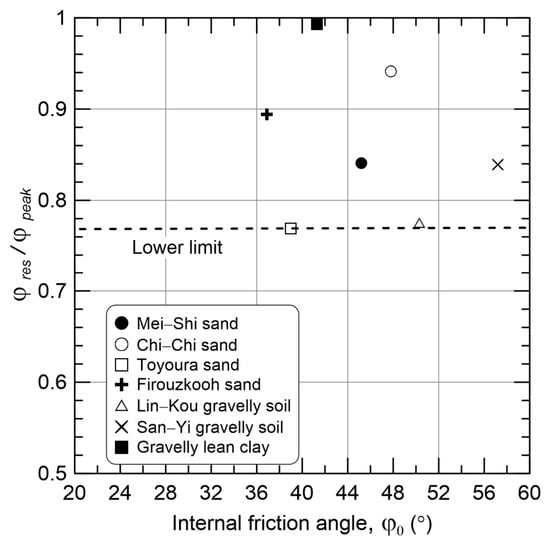
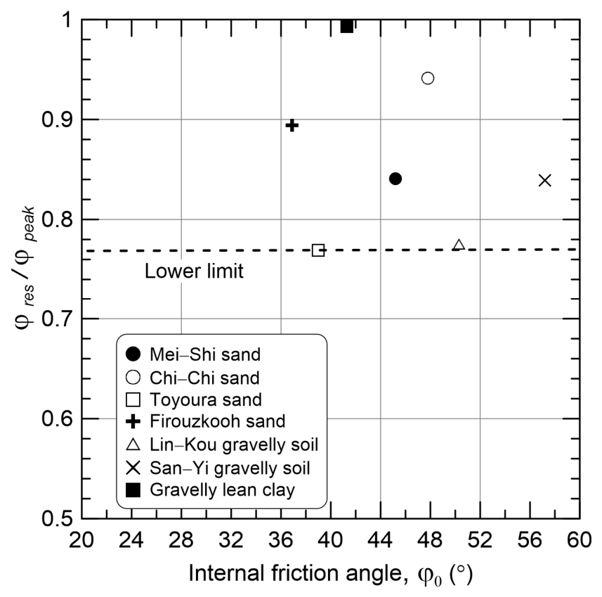
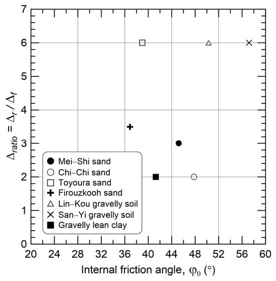
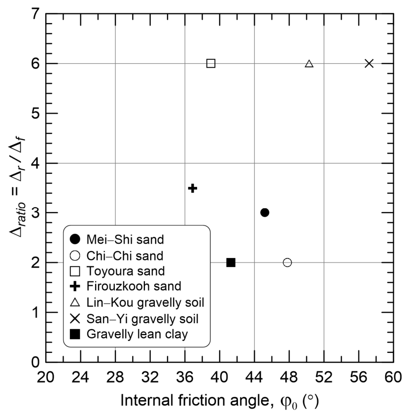
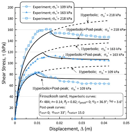
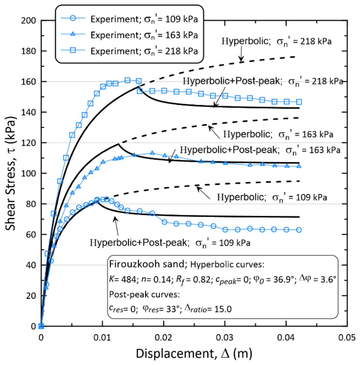
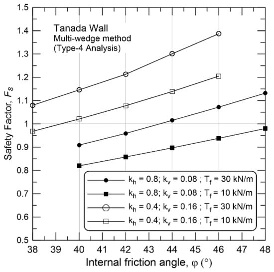
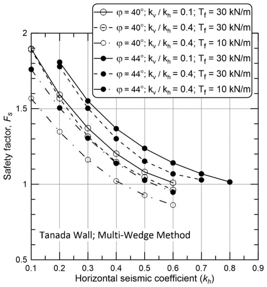
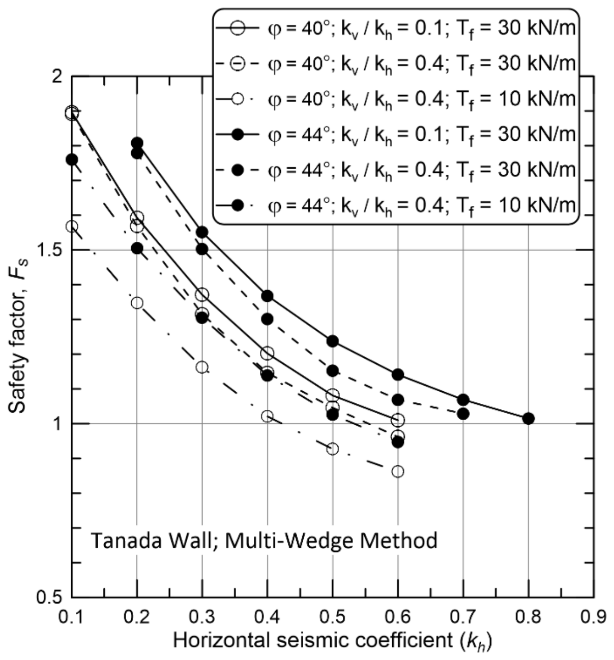
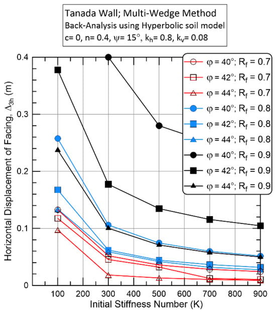
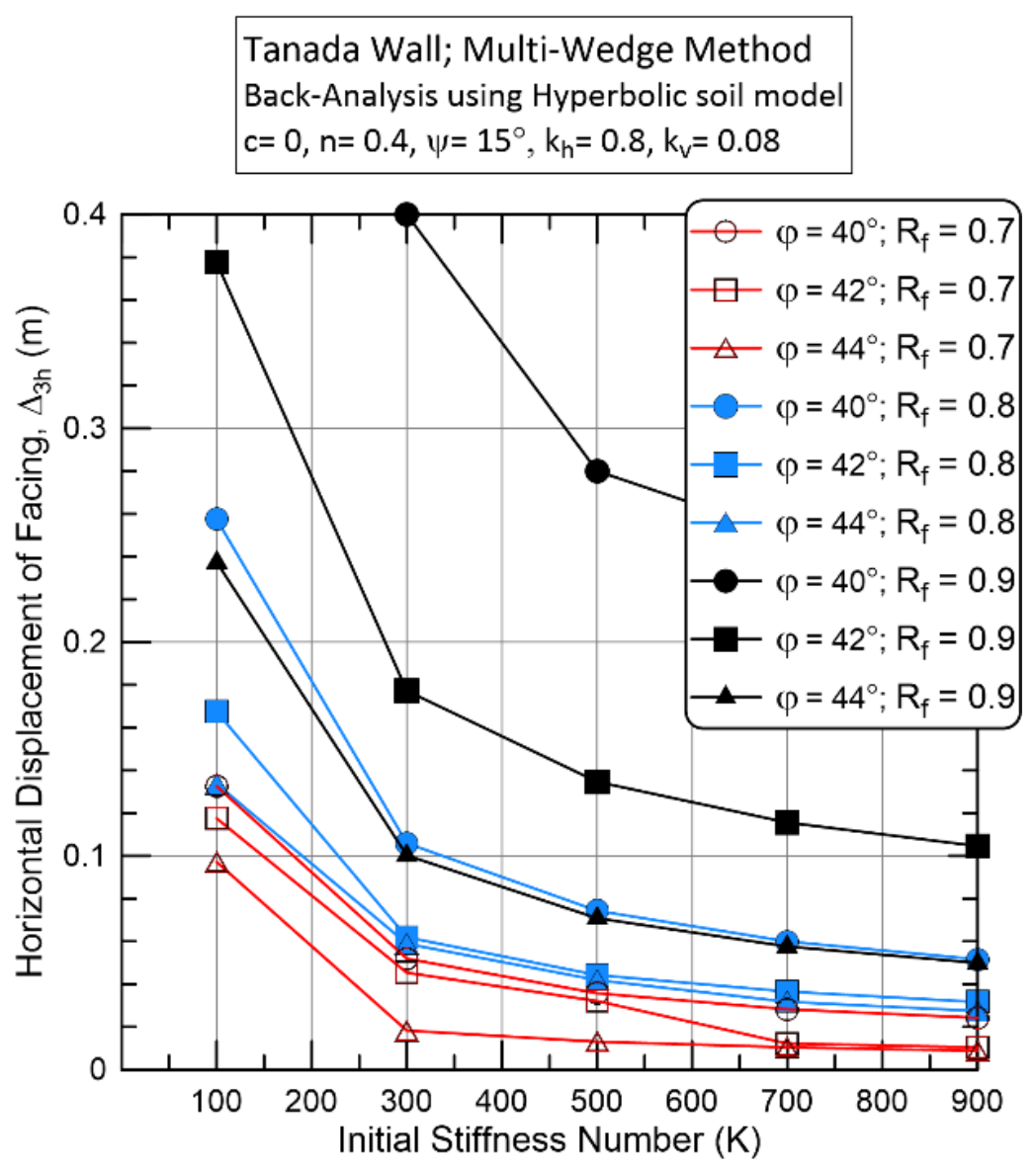
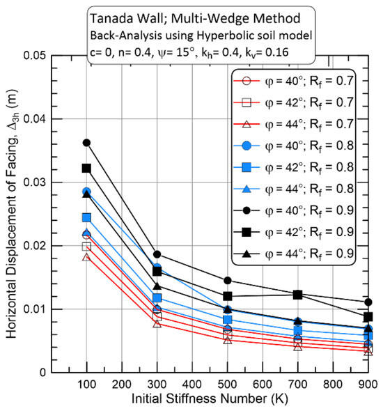
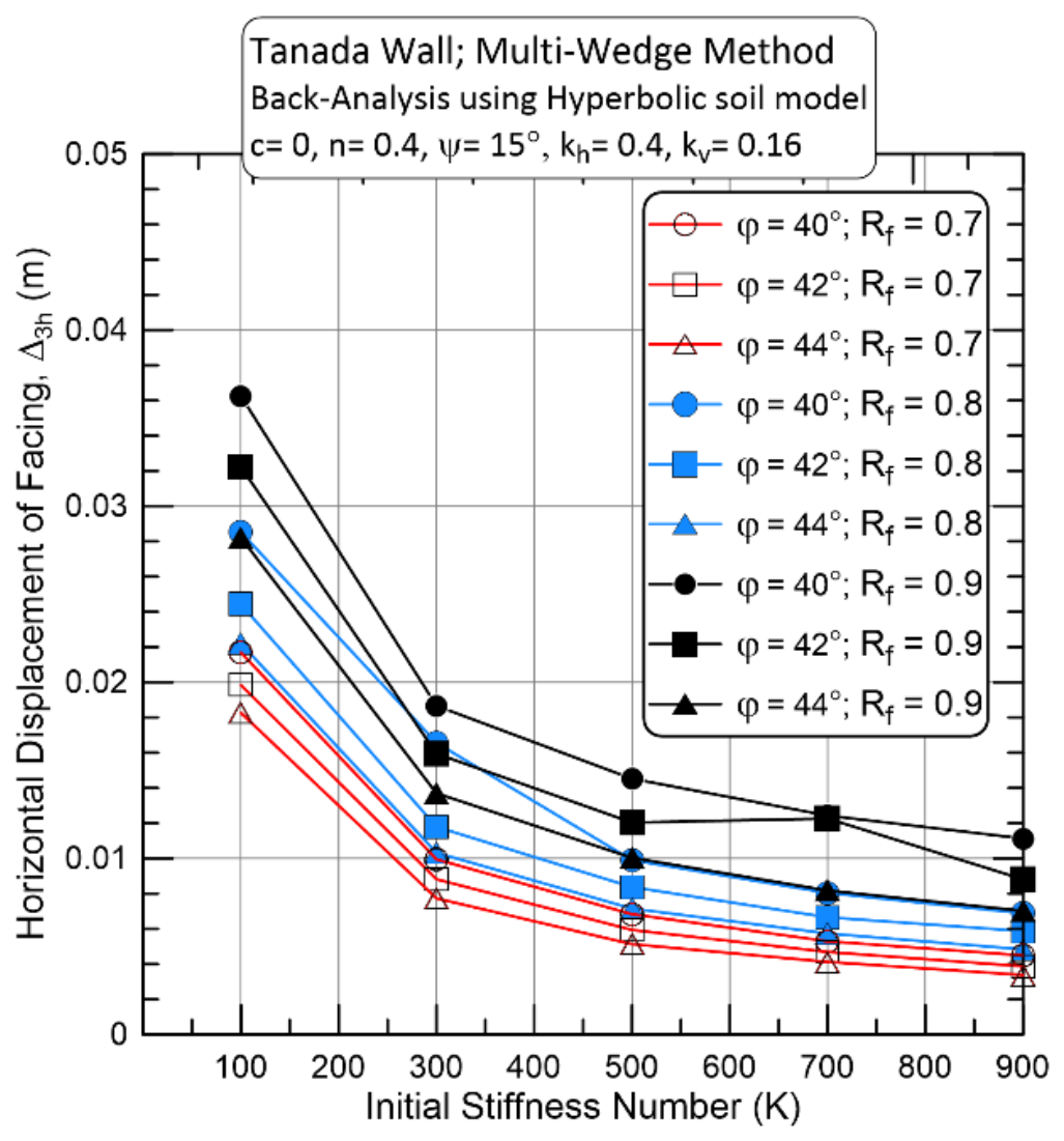
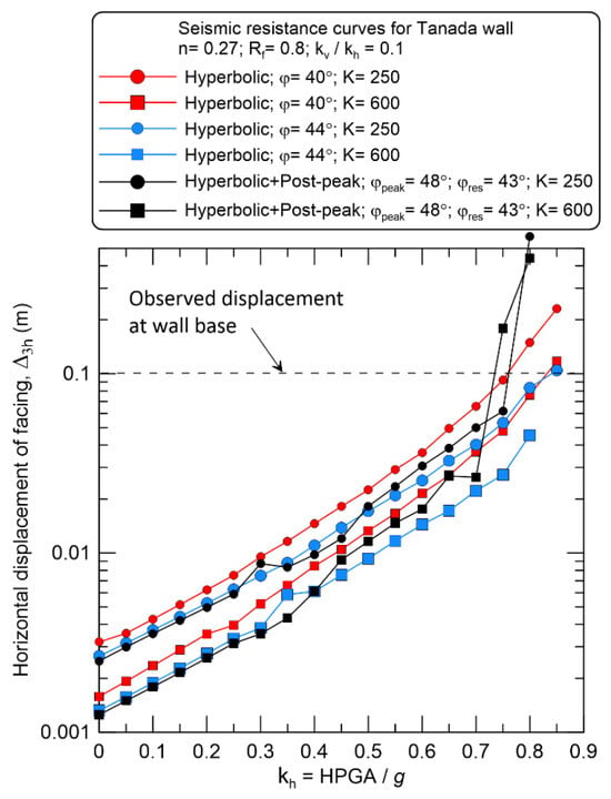
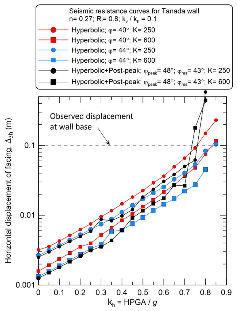
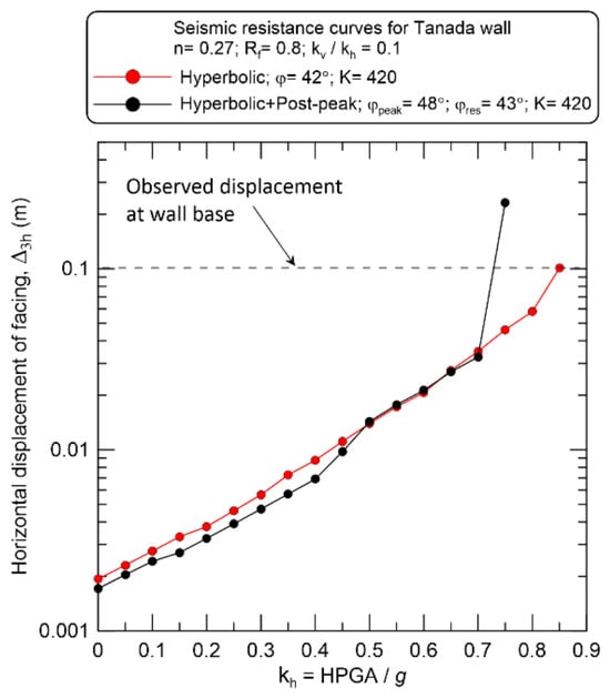
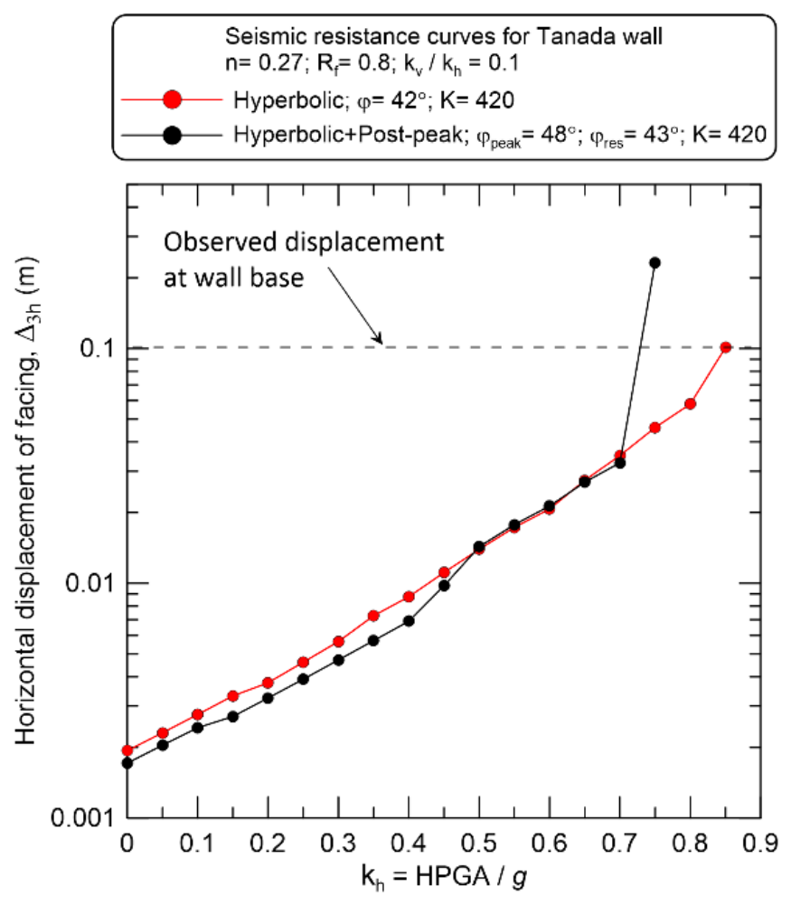
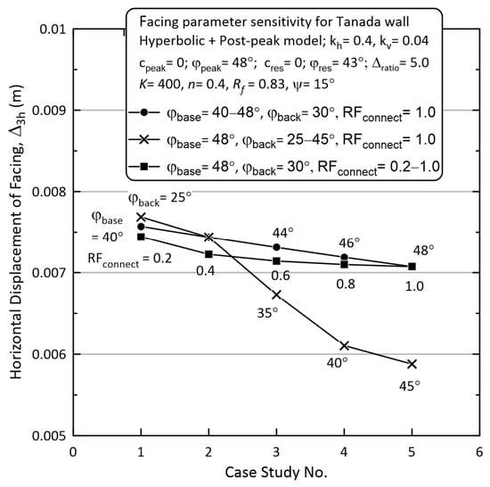
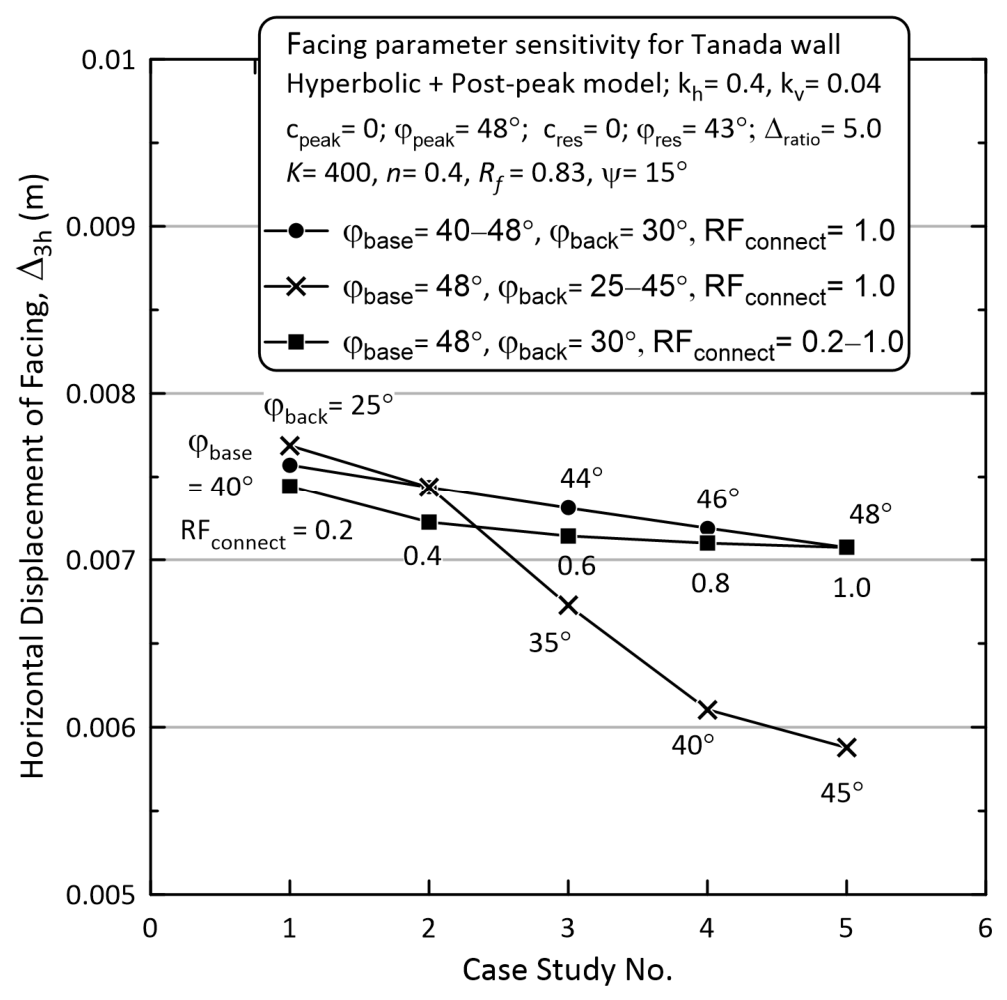

Disclaimer/Publisher’s Note: The statements, opinions and data contained in all publications are solely those of the individual author(s) and contributor(s) and not of MDPI and/or the editor(s). MDPI and/or the editor(s) disclaim responsibility for any injury to people or property resulting from any ideas, methods, instructions or products referred to in the content. |
© 2026 by the author. Licensee MDPI, Basel, Switzerland. This article is an open access article distributed under the terms and conditions of the Creative Commons Attribution (CC BY) license.