


Abstract
Subsurface faults in sediment-covered basins often lack clear surface expressions, necessitating integrated geophysical reconnaissance to identify structural complexities. The eastern margin of the Sofia Basin contains normal faults, with the geometry and activity of unmapped structures near Lozen Mountain being poorly understood. This study examines a presumed subsurface discontinuity using a ~216.2 m passive seismic profile across the Lozen Fault zone. Ambient vibrations from twelve point stations and a fixed reference station were analyzed to map structural anisotropy and wavefield variations using relative vertical-component spectral amplitudes, polarization parameters, and horizontal-to-vertical (H/V) spectral ratios. The spectral amplitude profiling revealed a significant lateral contrast of 6.21 dB across a depth interval of 0–140 m (p = 0.0043), suggesting a potential fault boundary. A two-level step model identified a horizontal transition at 109.0 m, with analyses indicating a zonal wavefield response. Southern stations recorded a more stable polarization axis (mean direction 37.32°) compared to the dispersed northern records (mean direction 60.43°, p = 0.097), while directional shifts in H/V distributions were significant (p = 0.0022). While these observations provide a clear structural indicator rather than direct proof of faulting, they effectively demonstrate that non-tectonic lithological and hydrological variations generate these identical spectral signatures. The results establish a well-constrained spatial target for future multi-profile surveys, electrical resistivity tomography, active-source seismic imaging, and paleoseismological trenches required to conclusively verify the geometry, age, and present-day activity of the fault structure.
1. Introduction
The Sofia Basin is an extensional intramontane graben structure bounded by systems of normal faults (see Figure 1) that have moved since the Holocene [1]. Along its southeastern margin, the basin abuts the northern flank of the Lozen Mountain, where the mapped Lozen fault has an approximately east–west regional trend and may comprise several short segments and subsidiary structures [1,2]. Geohelium anomalies and regional GNSS velocity and strain patterns indicate structural complexity in the eastern part of the basin [3,4,5]. Available short fault segments and subsidiary structures do not have a clear surface appearance, but show structural anisotropy and localized wave amplification in the frequency range of 2–5 Hz [6]. These regional observations motivate local investigation but, by themselves, do not establish the position, geometry, Quaternary age, or present-day activity of a specific structure north of Lozen Mountain. The use of non-destructive methods, e.g., microseismic sounding (MMS), contributes to the localization and characterization of local structures with changes in anisotropic properties.
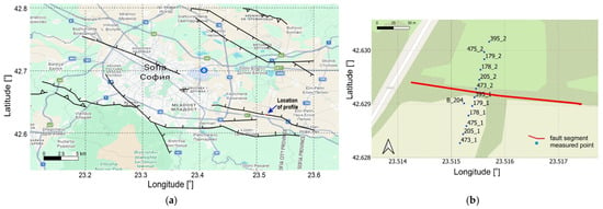
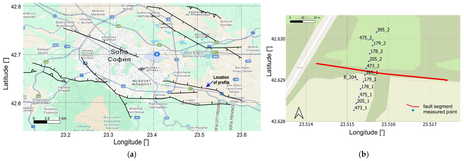
Figure 1.
Study area and measurement geometry: (a) location of the passive-seismic measurements in the southeastern part of the Sofia Basin (surrounding faults are depicted with the corresponding symbols in black); (b) the measured profile comprising twelve measurement positions and crossing the presumed subsurface fault structural zone. The fixed reference station B_204 is shown to the left of the measured points along the profile.
Subsurface structures in sediment-covered basins may have weak or absent surface expression. Active-fault databases and fault-characterization studies therefore integrate geomorphological mapping, paleoseismology, drilling, geodesy, and multiple geophysical methods [7,8,9,10,11,12,13]. Passive-seismic measurements are useful reconnaissance tools because they can identify lateral changes in spectral amplitude and directional wavefield properties without the need for artificial seismic sources. However, such anomalies are non-unique and may also reflect lithological changes, sediment thickness, water saturation, topography, anthropogenic disturbance, or variations in the ambient-noise source field. Passive-seismic observations alone should therefore be interpreted as evidence of a subsurface transition rather than as direct proof of an active fault.
In the present study, three complementary observables were derived from ambient-vibration recordings along a local southwest–northeast profile crossing a structural segment of the Lozen Fault: (1) relative spectral-amplitude levels referenced to a fixed base station, (2) three-component polarization parameters, and (3) azimuth-dependent H/V ratios. Microseismic spectral amplitudes are sensitive to lateral changes in elastic properties [14,15,16,17], whereas polarization and H/V rotation provide information about directional wavefield behavior and possible structural anisotropy [18,19,20,21,22,23,24,25,26,27,28,29]. Because all three observables were obtained from the same field experiment, their agreement represents internal methodological consistency rather than fully independent geological validation.
The primary objective of this study is to test whether the investigated profile contains a laterally coherent passive-seismic transition and to quantify its position, directional characteristics, uncertainty, and sensitivity to processing choices. We specifically evaluate (i) the north–south spectral-amplitude contrast and its spatial transition, (ii) axial polarization statistics and their confidence intervals, (iii) azimuthal H/V maxima and anisotropy indices, and (iv) sensitivity to frequency band, analysis-window length, overlap, quality-selection thresholds, and omission of individual stations. This study focuses on identifying the primary structural characteristics while leaving the determination of dip, along-strike continuity, Quaternary age, slip rate, and present-day activity for future investigations. These properties require co-registered independent geophysical imaging and geological or paleoseismological validation. Accordingly, the results are discussed as evidence for a local fault-related subsurface transition and as a basis for subsequent intersecting profiles, electrical-resistivity or active-source seismic imaging, borehole constraints, and analysis of local seismicity.
2. Methods
2.1. Relative Microseismic Spectral-Amplitude Profiling
Relative microseismic spectral-amplitude profiling was used to identify lateral changes in the ambient seismic field along the investigated profile. Geological heterogeneities may modify the amplitude spectrum of the surface wavefield by altering elastic properties, attenuation, scattering, and local resonance [14,15,16,17]. Consequently, lateral spectral-amplitude contrasts may indicate a change in subsurface structure, although they cannot be interpreted uniquely as a seismic-velocity contrast.
The analysed quantity is expressed as the relative spectral-amplitude level according to:
where Ai(xi,f) is the spectral amplitude at profile position xi, Abase(f) is the simultaneous spectral amplitude at the fixed reference station, and LA is expressed in decibels (dB). Positive values indicate higher spectral amplitudes relative to the reference station, whereas negative values indicate lower relative amplitudes. The resulting field is therefore an amplitude-ratio representation and not a direct image of seismic velocity.
For visualization, the frequency was converted to an apparent depth coordinate using the quarter-wavelength relation:
where cR(f) is the adopted frequency-dependent Rayleigh-wave phase velocity.
For the topographic representation in Figure 2, the apparent-depth coordinate was converted to elevation above sea level according to the following Equation:
where zsurf(xi) is the local ground-surface elevation at profile station i, and Happ(f) is the apparent depth obtained from Equation (2). Thus, the apparent depth is measured downward from the local topographic surface. The coefficient 0.25 was not calibrated locally, and the transformed vertical coordinate is therefore referred to as apparent depth rather than calibrated geological depth. To assess the influence of this assumption, the analysis was repeated using coefficients of 0.40, 0.45, and 0.50. This sensitivity test evaluates whether the lateral amplitude contrast and its horizontal position remain stable when the apparent depth scale is changed.
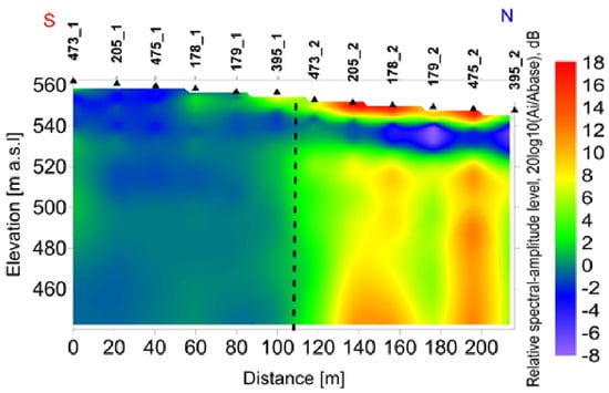
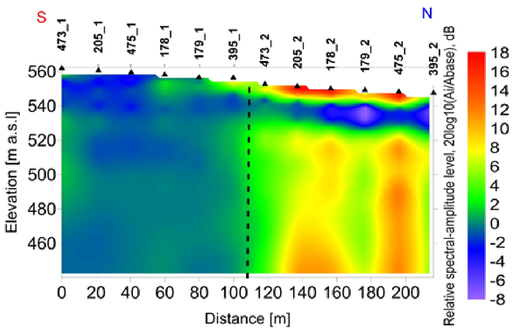
Figure 2.
Relative microseismic spectral-amplitude level along the measured profile.
2.2. Reference-Station Spectral Processing and Spatial Analysis
During each measurement session, the mobile profile stations and the fixed reference station B_204 operated simultaneously. A common 90 min interval was selected from each approximately 2 h recording session to reduce the influence of differences in recording duration. The vertical component was used for the relative spectral-amplitude analysis, whereas all three components were retained for the polarization and H/V-rotation analyses.
The same spectral-processing sequence was applied to the profile and reference records. At each frequency, the spectral amplitude obtained at a profile station was divided by the simultaneous spectral amplitude at B_204 and converted to decibels using Equation (1). Referencing all mobile measurements to the fixed station reduces the influence of temporal variations in the ambient-noise level between the two successive recording sessions.
The selected 90 min vertical-component records, sampled at 100 Hz, were demeaned and linearly detrended, then divided into contiguous, non-overlapping windows of 8192 samples, corresponding to 81.92 s. Each window was tapered using a Hann window and transformed using an 8192-point fast Fourier transform, providing a raw frequency resolution of approximately 0.0122 Hz. For each profile station and the corresponding simultaneous B_204 record, the one-sided amplitude spectra from the 65 complete windows were arithmetically averaged. The mean spectrum of each profile station was subsequently divided by the mean spectrum of the corresponding B_204 record. The resulting spectral-amplitude ratios were interpolated onto a logarithmic grid of 252 frequencies between 0.100619 and 49.4733 Hz, with an adjacent-frequency ratio of approximately 1.025. No additional Konno–Ohmachi or moving-average smoothing was applied beyond this logarithmic frequency regridding.
The relative spectral-amplitude values were first assigned to the measured profile distances and to the apparent-depth coordinate defined by Equation (2). For Figure 2, each apparent-depth value was subsequently converted to elevation above sea level by subtracting it from the local ground-surface elevation of the corresponding station. Values between adjacent measurement positions were represented by piecewise-linear interpolation in the profile-distance–elevation plane. No extrapolation was applied beyond the first and last profile stations, and no spatial smoothing was used in the primary quantitative analysis.
The principal lateral transition was evaluated from the station-averaged spectral-amplitude levels using a two-level step model. All candidate divisions retaining at least three measurement stations on either side were tested. The preferred division was defined as the solution with the minimum within-group sum of squared residuals. Positional stability was assessed using 10,000 frequency-block bootstrap realizations. The resulting position is therefore reported as a transition interval rather than as an exact fault trace.
2.3. Three-Component Polarization Analysis
Three-component polarization analysis was applied to characterize the directional properties of the ambient seismic wavefield [18,19,20]. The method identifies the principal axes of particle motion within successive time windows but, by itself, does not determine the geological origin or present-day activity of the structure producing the directional response.
The north, east, and vertical components were divided into 10 s windows with 50% overlap. After removing the mean value from each component, a 3 × 3 covariance matrix was calculated for each window. Eigenvalue decomposition yielded ordered eigenvalues:
and their corresponding eigenvectors. The first eigenvector defines the direction of maximum variance. Its horizontal azimuth was measured clockwise from geographic north and reduced to the axial interval 0–, because orientations and are equivalent.
Linearity was calculated as:
where and are the first and second eigenvalues of the covariance matrix. Values of L approaching 1 indicate predominantly linear particle motion.
Planarity was calculated as:
where is the third eigenvalue. Larger values of indicate a stronger planar contribution to the particle motion.
Windows retained for the primary polarization analysis were required to satisfy:
and
where is the linearity parameter defined by Equation (3) and is the inclination of the principal eigenvector relative to the horizontal plane. Planarity , defined by Equation (4), was calculated for every window and retained as a diagnostic parameter. The originally stated condition was non-restrictive for the present dataset and is therefore not treated as an effective independent selection criterion.
The sensitivity of the window selection was evaluated using operational loose and strict alternatives. The loose selection used and . The strict selection used , , and . Additional one-at-a-time tests evaluated linearity thresholds of 0.50, 0.60, and 0.70; inclination thresholds of , , and ; and planarity thresholds of 0.20, 0.30, 0.50, and 1.00.
Axial dispersion was calculated after the accepted windows had been grouped by station or zone and was used as a descriptive measure of directional concentration rather than as an additional per-window acceptance criterion.
Polarization was examined in the frequency ranges of 0.4–0.6 Hz, 0.9–2.0 Hz, 2.5–7.0 Hz, and 0.2–20 Hz. Directional changes between these bands were treated as frequency-dependent characteristics of the ambient wavefield. Stable polarization was interpreted as evidence of directional structural control, but not as direct proof of a fault, its age, or its present-day activity.
2.4. Axial Statistics, Uncertainty, and Sensitivity Tests
Axial statistics were calculated by doubling the polarization azimuths before computing the circular statistics and subsequently halving the resulting mean direction. For axial observations , the doubled-angle components were calculated as:
The mean axial direction and mean resultant length were then obtained from:
Circular variance was calculated as:
and axial circular standard deviation according to the following Equation:
The final angular quantities were expressed in degrees.
Two levels of statistical analysis were distinguished. Window-level statistics describe the complete population of accepted polarization windows. Because successive 10 s windows overlap by 50%, their uncertainty was evaluated using a stratified moving-block bootstrap rather than by treating all windows as statistically independent. A total of 10,000 bootstrap realizations were generated using blocks of 12 consecutive windows, corresponding to 60 s of recording time. Every measurement record was resampled separately.
The primary comparison between the southern and northern profile groups was performed at station level. A mean axial direction was first calculated for each of the twelve profile stations, after which every station was assigned equal weight. The fixed reference station B_204 was excluded from this spatial comparison because it remained at the same position during the two recording sessions. The north–south difference was evaluated using an exact permutation test over all possible divisions into two six-station groups.
Processing sensitivity was evaluated by comparing alternative quality thresholds; 10 and 20 s windows; the original 50% overlap and a decimated, non-overlapping sequence; four frequency ranges; and leave-one-station-out solutions. The exported results were not sufficient to reconstruct 5 s windows with exact overlap at 25% and 75%. These additional combinations require reprocessing of the original three-component recordings.
2.5. Azimuthal H/V-Rotation Analysis
Azimuth-dependent H/V ratios were calculated to examine directional variations in the ambient-vibration response [27,28,29,30,31]. The two horizontal components were rotated clockwise from geographic north, and an H/V value was obtained for every analysed frequency and azimuth. Because H/V orientation is axial, the quantitative analysis used the independent interval 0– at increments. Values ranged from to in the exported plotting matrices, and there are mirrored repetitions that were not treated as independent azimuths.
The primary quantitative analysis was conducted in the 2.5–7.0 Hz band, corresponding to the available discrete frequencies from 2.55568 to 6.86217 Hz. At each station, the H/V values were averaged over the selected frequency range for every azimuth. The dominant axial direction was defined as the maximum of the frequency-averaged directional curve. A local quadratic interpolation through the maximum and its two neighboring azimuth samples was used to estimate the peak direction between the grid values.
Directional H/V strength R was quantified using the maximum-to-minimum ratio:
and the normalized anisotropy index:
The stability of the peak direction across the frequency band was quantified using the axial resultant length of the individual frequency-peak directions, weighted by their frequency-specific anisotropy indices. Directional confidence intervals and uncertainty in were estimated using 5000 moving-block bootstrap realizations over neighboring frequency bins.
Zone-level H/V directions were calculated from the six profile stations in each group, assigning equal weight to every station. The fixed reference station B_204 was analyzed as a quality-control record but excluded from the spatial north–south comparison. Differences in station-level directions and in mean anisotropy indices were evaluated by exact permutation of the twelve station labels.
3. Field Measurements Along a Profile Crossing the Presumed Fault Structural Zone
Microseismic field measurements were conducted in August 2025 along a ~216.2 m SW–NE-oriented profile north of Lozen village, shown in Figure 1. The profile comprised twelve measurement positions with a mean spacing of approximately 20 m. The ground-surface elevation of each measurement position was determined geodetically and was used to place the apparent-depth values in absolute elevation coordinates in Figure 2. Six profile stations were operated during each of two successive measurement sessions, along with a fixed reference station located close to the profile stations. Seven ETNA-2 accelerometers were therefore used during each session. The horizontal sensor axes were oriented towards geographic north and east. The fixed reference station, denoted B_204, is not treated as an independent profile position in the spatial statistical comparisons.
The southwestern group of six profile stations was recorded from 05:27 to 07:27 GMT, and the northeastern group was recorded from 07:51 to 09:51 GMT. Each measurement session lasted approximately 2 h. The reference accelerometer B_204 remained at the same location during both sessions and provided the corresponding reference spectrum for the mobile profile stations.
Ambient-vibration recording duration was assessed, and sensor deployment was carried out following the general recommendations of SESAME [28] and Chatelain et al. [29]. Conventional H/V processing and the rotational H/V exports were generated using the Geopsy software package [31], whereas the covariance-based polarization, axial-statistical, bootstrap, permutation, and sensitivity analyses were performed using dedicated MATLAB R2024b scripts.
4. Results
4.1. Relative Spectral-Amplitude Profile Determination
For every profile station i, the spectral amplitude was referenced to the simultaneously operating reference station B_204 and calculated using Equation (1). For the discrete-velocity model, we assumed cR = 700 ms−1 for frequencies from 0.100619 to 9.93847 Hz, cR = 550 ms−1 for frequencies from 10.1869 to 19.8421 Hz, and cR = 360 ms−1 for frequencies from 20.3382 to 49.4733 Hz. Figure 2 presents the relative microseismic spectral-amplitude level along the 216.2 m profile. Colors represent in dB, where is the spectral amplitude at each profile station and is the simultaneous spectral amplitude at the fixed reference station B_204. The vertical axis shows elevation above sea level. For each station and frequency, the elevation was calculated by subtracting the apparent depth , derived from Equation (2), from the local ground-surface elevation. The upper boundary follows the local topography. Values between adjacent stations are represented by piecewise-linear interpolation in the profile-distance–elevation plane. The dashed vertical line marks the preferred lateral transition at 109.0 m along the profile, and the shaded interval between 99.8 m and 118.2 m represents the minimum lateral uncertainty imposed by the station spacing.
Across the 0–140 m apparent depth interval, the mean relative spectral-amplitude level was −0.01 dB for the six southern profile stations and 6.21 dB for the six northern stations. The north–south difference was 6.21 dB, corresponding to a 2.04-fold ratio of geometric-mean spectral amplitudes. An exact station-level permutation test yielded . A nested station and frequency-block bootstrap produced a 95% confidence interval of 2.83–9.80 dB for the north–south contrast.
The positive north–south contrast was observed in most apparent depth intervals. It reached 7.90 dB at 0–10 m, 5.40 dB at 20–40 m, 6.75 dB at 40–80 m, and 8.02 dB at 80–140 m. The 10–20 m interval was the only exception, with a non-significant difference of −2.22 dB (p = 0.132). This interval coincides with the transition between two values in the adopted piecewise Rayleigh-wave velocity model and is therefore interpreted cautiously.
A two-level step model fitted to the station-averaged values located the principal lateral transition at a profile distance of 109.0 m. This position lies within the unsampled interval between the stations at 99.8 and 118.2 m. The station geometry therefore constrains the nominal transition to 109.0 ± 9.2 m. Frequency-block bootstrap resampling selected this boundary in 72.54% of the realizations, while adjacent solutions extended the conservative transition zone to approximately 89.8–127.6 m. The preferred step model explained approximately 64.3% of the variation between the station means.
Repeating the analysis with depth-scaling coefficients of 0.40, 0.45, and 0.50 preserved the lateral amplitude contrast and its horizontal transition, but changed the assigned apparent depth scale. A feature shown at 140 m with a coefficient of 0.25 would correspond to approximately 224–280 m for coefficients between 0.40 and 0.50. The lateral transition is therefore more robustly constrained than its vertical extent.
Although Figure 2 is displayed in absolute elevation coordinates, the quantitative comparison in Table 1 is grouped by apparent depth below the local ground surface.
Table 1.
North–south relative spectral-amplitude contrast by apparent depth interval.
4.2. Polarization Results and Processing Sensitivity
For spatial comparison, the twelve profile stations were divided into a southern group comprising the six stations with suffix “_1” and a northern group comprising the six stations with suffix “_2”. The reference station B_204 was excluded from the spatial statistics because it occupied the same position during both recording sessions.
The baseline selection criteria retained 1345 of 12,725 profile windows, corresponding to 10.57% of the analyzed windows. In the southern group, 808 of 6480 windows were accepted (12.47%), whereas 537 of 6245 windows were accepted in the northern group (8.60%). The lower acceptance rate in the northern records is consistent with their greater directional dispersion.
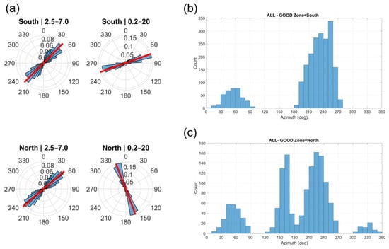
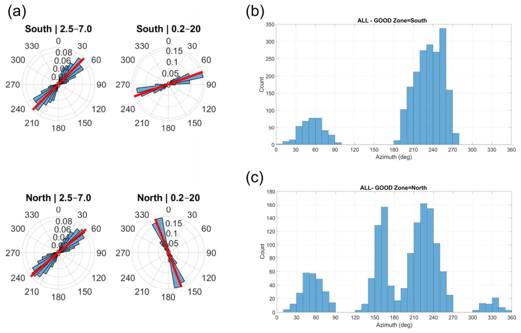
The axial polarization distributions studied in the frequency ranges 2.5–7.0 Hz and 0.2–20 Hz bands for all points along the profile are depicted in Figure 3a, and the corresponding azimuth histograms for the south and north GOOD zones are depicted in Figure 3b and Figure 3c, respectively. No windows satisfied the complete baseline selection in the 0.4–0.6 Hz and 0.9–2.0 Hz bands. This result is interpreted as a consequence of the adopted quality criteria, the limited recording duration, signal-to-noise conditions, and temporal variability of the ambient sources. It is not treated as evidence that the low-frequency wavefield is isotropic.
Figure 3.
Axial polarization distributions for the profile stations: (a) rose diagrams for the 2.5–7.0 Hz and 0.2–20 Hz bands; (b) histogram of accepted polarization azimuths for the northern group; (c) histogram for the southern group. Orientations separated by represent the same axial direction.
The accepted polarization windows showed a more concentrated axial distribution in the southern group than in the northern group. Excluding the reference station B_204, the pooled mean axial direction for the southern records was , with mean resultant length R = 0.624 and a 95% moving-block-bootstrap confidence interval of –. The northern records yielded a mean axial direction of , a lower resultant length of R = 0.377, and a wider 95% confidence interval of –.
For all twelve profile records combined, the mean axial direction was , with and a 95% confidence interval of –. An exact record-level permutation test yielded . Thus, the northern distribution is shifted and substantially less concentrated than the southern distribution, but the difference does not reach the 5% significance level in this primary polarization comparison. Peaks separated by , for example, near and , represent the same axial orientation. These peaks should not be described as orthogonal or as two separate polarization directions. Additional peaks in the northern distribution indicate directional complexity, but their geological origin cannot be determined uniquely from the present data.
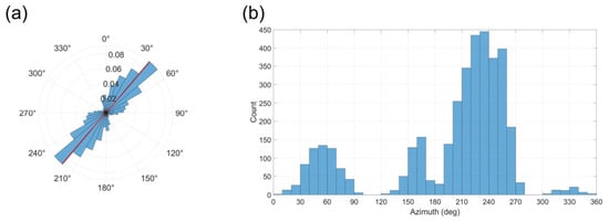
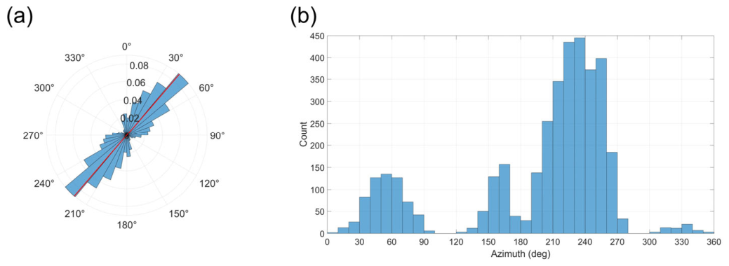
The aggregated distribution in Figure 4 summarizes all accepted profile windows. Its dominant axial mode lies within the approximately – sector, consistent with the combined doubled-angle mean of . Because the northern records are substantially more dispersed than the southern records, the aggregated rose diagram is partially dominated by the more concentrated southern contribution and should not be interpreted as evidence of a single, uniform profile-wide orientation.
Figure 4.
Aggregated axial polarization distribution for the twelve-point records: (a) rose diagram of all accepted windows; (b) corresponding azimuth histogram. The fixed reference station B_204 is excluded. Azimuths differing by represent the same axial orientation.
Under the interpretative assumption that the preferred horizontal polarization is approximately normal to a fault-related structure, the orthogonal direction corresponding to the combined mean axis is , with a bootstrap interval of –. This value is an inferred orientation and not a direct measurement of fault strike. Leave-one-station-out solutions produced orthogonal directions between and , indicating that between-station sensitivity is wider than the formal pooled-window confidence interval.
The confidence intervals were obtained by stratified moving-block bootstrap resampling. B_204 was excluded because it was a fixed reference station rather than an independent profile position. Nonetheless, the polarization results are in very good agreement with geological observations and with the mapped fault geometry shown on the Geological Map of Bulgaria, Sofia Sheet [32].
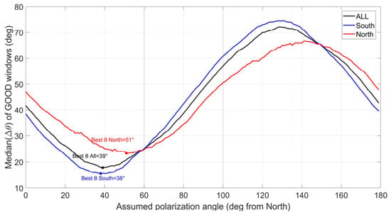
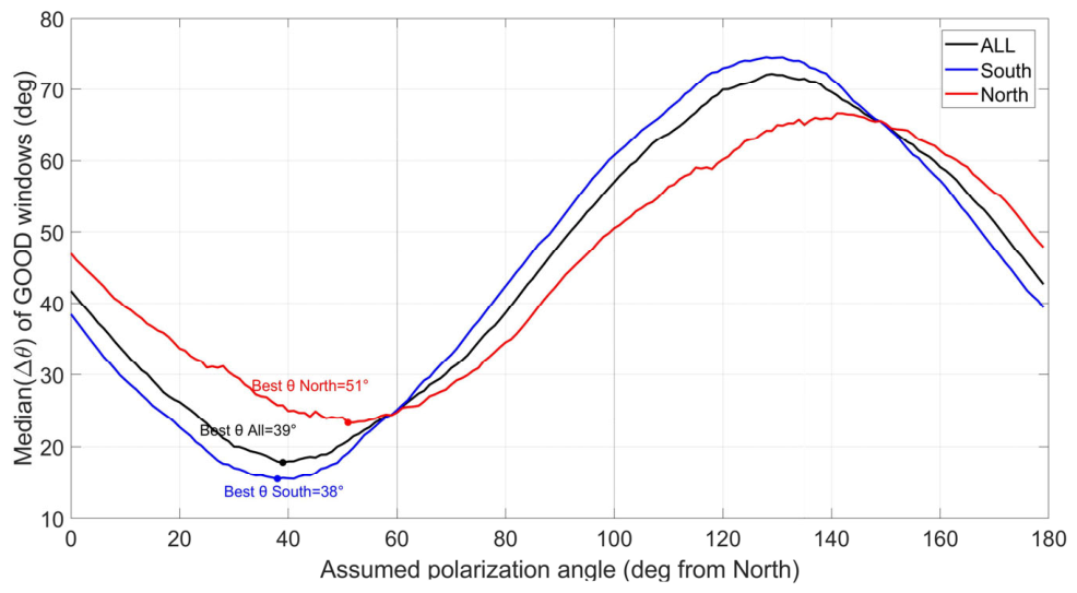
Figure 5 shows the median axial misfit between the observed polarization and a sequence of trial orientations. The descriptive minima occur near for the southern records, for the northern records, and for the combined set. These values are broadly consistent with the window-level axial statistics, but the wider station-level and processing-sensitivity results indicate that the inferred orientation is not uniform along the profile. The sweep analysis is therefore used as a descriptive visualization and not as an independent or more precise estimator of structural strike.
Figure 5.
Median axial misfit between the observed polarization azimuths and trial polarization orientations for the southern, northern, and combined point records. The minima describe preferred polarization axes and do not directly represent fault strike.
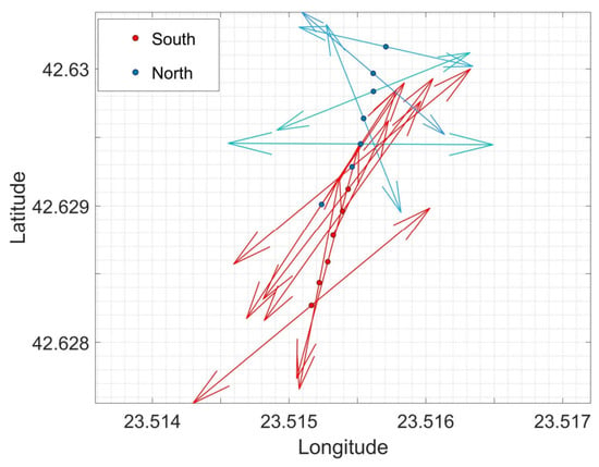
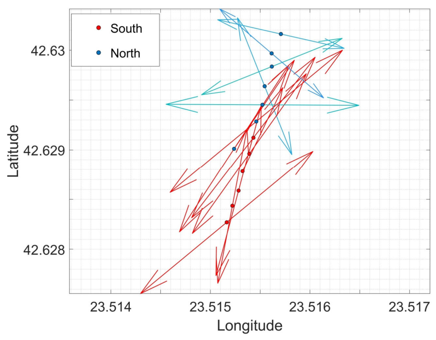
Figure 6 shows the station-level mean axial polarization directions along the profile. The southern stations form a comparatively coherent directional group, whereas the northern stations show greater azimuthal variability and lower directional concentration. This spatial pattern is consistent with a change in the directional properties of the ambient wavefield, but it does not define a unique fault trace or prove that the observed variability is caused exclusively by fault-related fracturing.
Figure 6.
Station-level mean axial polarization directions along the passive-seismic profile. Arrow orientation represents the mean axial direction, and arrow length or color represents the mean resultant length R. Southern and northern profile stations are shown using different symbols. The fixed reference station B_204 is excluded from the spatial comparison.
Because each profile station was assigned equal weight in the sensitivity tests, the station-weighted group directions reported below differ from the pooled-window estimates presented in Table 2.
Table 2.
Pooled axial statistics of GOOD polarization windows from the twelve-point records.
The polarization result was further evaluated against the processing choices. Across the operational loose, baseline, and strict quality-threshold sets, the station-weighted southern mean remained within –, whereas the northern mean varied between approximately and . The northern records are therefore considerably more sensitive to the selection criteria than the southern records.
For all 10 s windows, changing from 50% overlap to a decimated non-overlapping sequence changed the combined mean direction from to . Using all windows, the combined mean directions obtained from 10 and 20 s windows were and , respectively. The principal all-window mid-frequency direction is therefore relatively insensitive to window length and overlap. In contrast, the filtered northern and combined results were less stable because considerably fewer windows satisfied the quality criteria.
The directional response was strongly frequency dependent. In the 20 s all-window analysis, the 0.4–0.6 Hz and 0.9–2.0 Hz bands yielded combined axes of and , respectively, without significant north–south differences. The 2.5–7.0 Hz band yielded a combined axis of and a significant group difference . The broad 0.2–20 Hz result was poorly concentrated . Consequently, the structural interpretation is restricted to the 2.5–7.0 Hz mid-frequency response and is not extrapolated to the complete frequency range.
Leave-one-station-out analysis produced combined polarization axes between and , corresponding to orthogonal directions between and . No individual station therefore controls the complete result, although the spread confirms that a single precise structural orientation is not warranted.
4.3. Azimuthal H/V-Rotation Results
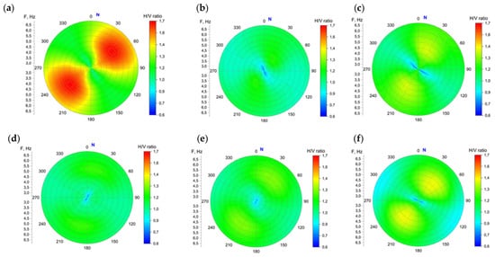
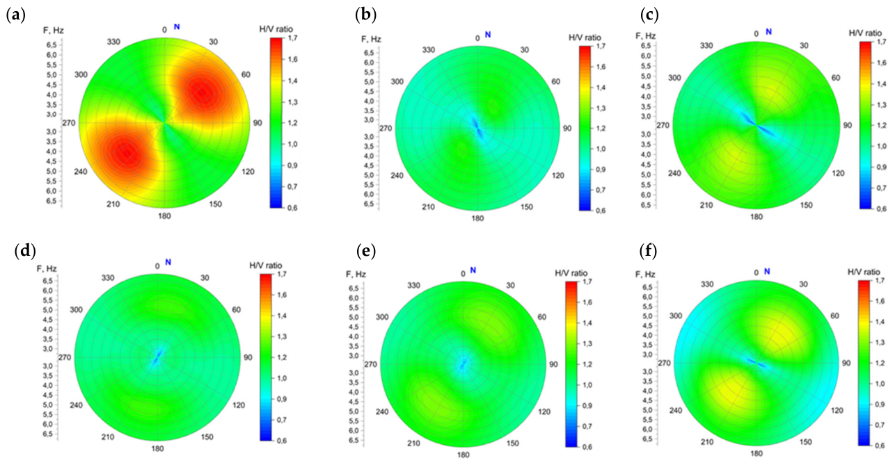
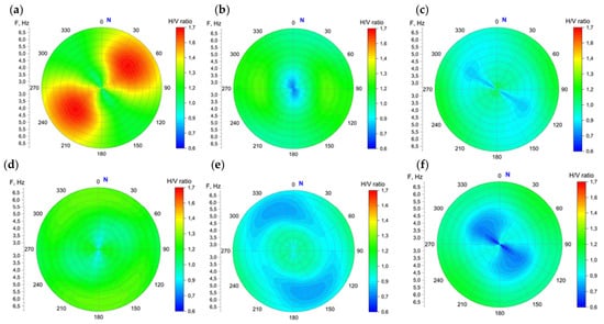
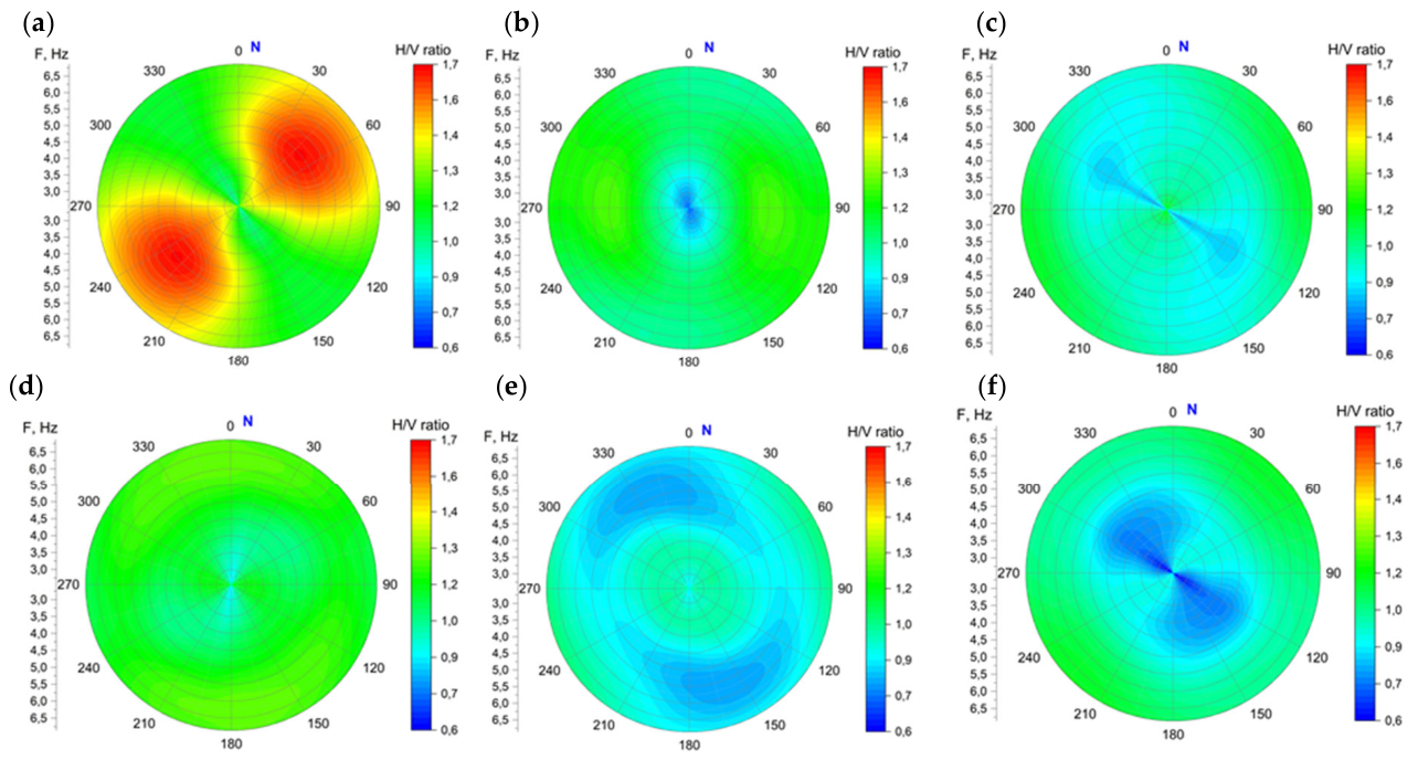
The results of the calculated values of the azimuth-dependent HB ratio for each station of the AB profile are presented graphically in Figure 7 and Figure 8, respectively, for the southern and northern stations located relative to the fault segment. To provide a direct visual comparison, all panels are plotted using the same H/V color scale (0.6 to 1.7), the same frequency range, azimuthal convention, and identical color bar intervals.
Figure 7.
Azimuth-dependent H/V ratios for the six southern profile stations: (a) 473_1, (b) 205_1, (c) 475_1, (d) 178_1, (e) 179_1, and (f) 395_1. All panels use the same H/V color scale from 0.6 to 1.7, identical frequency and azimuth axes, and the same clockwise azimuth convention relative to geographic north.
Figure 8.
Azimuth-dependent H/V ratios for the six northern profile stations: (a) 473_2, (b) 205_2, (c) 475_2, (d) 178_2, (e) 179_2, and (f) 395_2. The color scale and the azimuth convention are the same as in Figure 7.
The H/V-rotation matrices depicted in Figure 7 show substantial station-to-station variation in both preferred azimuth and anisotropy strength. The quantitative comparison was performed in the 2.5–7.0 Hz band using the independent axial interval –. The six southern stations yielded a station-weighted mean axial direction of , with resultant length and a 95% station-bootstrap interval of –. The corresponding mean anisotropy index was . The six northern stations yielded a mean axial direction of , with , a 95% interval of –, and mean .
An exact station-label permutation test indicated a significant difference between the southern and northern H/V directional distributions . In contrast, the mean anisotropy indices did not differ significantly . Thus, the two profile groups differ in preferred H/V direction, but not in their average anisotropy strength.
Strong and directionally stable H/V anisotropy was observed at stations 395_1, 395_2, 473_2, and 475_1. Station 178_1 showed the weakest response, with and frequency-direction stability ; its individual peak direction is therefore not interpreted as a reliable structural orientation.
These results demonstrate a zonal change in azimuthal H/V response rather than one uniform preferred direction throughout the profile (see Table 3). If the H/V maximum is assumed to be approximately normal to a fault-related structure, the corresponding orthogonal directions would be for the southern group and for the northern group. Because this conversion depends on the physical origin of the directional H/V response, these values are treated as interpretative orientations and not as direct measurements of fault strike.
Table 3.
Quantitative azimuthal H/V characteristics in the 2.5–7.0 Hz band.
5. Discussion
5.1. Integrated Interpretation of the Passive-Seismic Observations
The three passive-seismic observables identify a laterally coherent change within the central part of the investigated profile, although they respond to different properties of the ambient wavefield. The relative spectral-amplitude analysis reveals a statistically significant north–south contrast of 6.21 dB across the 0–140 m apparent depth interval. The preferred horizontal transition is centered at approximately 109 m along the profile and is constrained by the station geometry to the interval between 99.8 and 118.2 m. Frequency-block resampling indicates a broader conservative transition zone of approximately 89.8–127.6 m. The horizontal position of the contrast is more robust than its apparent depth extent, which depends directly on the adopted Rayleigh-wave velocity model and apparent depth-scaling coefficient.
The polarization results do not support one completely uniform directional response along the profile. The southern records exhibit a more concentrated axial distribution, whereas the northern records are more dispersed and have a shifted mean orientation. In the primary baseline analysis, the exact permutation test yielded ; therefore, the polarization difference is suggestive but does not reach the 5% significance level. The sensitivity tests further show that the southern direction is comparatively stable, while the northern result varies more strongly with the quality-selection thresholds and with the reduced number of accepted windows.
The azimuthal H/V analysis provides a complementary directional observable. In the 2.5–7.0 Hz band, the station-level H/V directions differ significantly between the southern and northern groups , whereas the mean anisotropy indices do not differ significantly . This indicates a change in the preferred direction of the H/V response rather than a systematic increase in anisotropy strength from one side of the profile to the other. The greater directional dispersion in the northern group is observed in both the polarization and H/V analyses, although the two techniques do not yield identical mean directions.
Under the interpretative assumption that the dominant horizontal polarization is approximately normal to a fault-related structure, the combined polarization mean corresponds to an orthogonal orientation of approximately . Leave-one-station-out solutions, however, range from approximately to . Furthermore, the H/V-derived orthogonal directions differ between the southern and northern groups. Consequently, the data do not justify describing , , or any other single value as a precisely measured fault strike. These orientations are processing- and mechanism-dependent structural estimates.
5.2. Frequency Dependence and Processing Robustness
The directional interpretation is frequency dependent. The clearest processing-stable response is observed in the 2.5–7.0 Hz band. The lower-frequency ranges of 0.4–0.6 Hz and 0.9–2.0 Hz yield substantially different mean orientations and do not show statistically significant north–south differences in the available all-window analysis. The broad 0.2–20 Hz result has low directional concentration and combines wavefield contributions with potentially different origins.
The 10 and 20 s all-window analyses yield similar combined mid-frequency directions, and removal of the 50% overlap changes the all-window mean by less than . Thus, the principal all-window mid-frequency orientation is not created solely by the selected window length or by overlap. In contrast, the quality-filtered northern and combined results are less stable because only a limited fraction of the available windows satisfies the baseline criteria. These observations require the interpretation to be restricted to the mid-frequency response. The preferred orientation should not be extrapolated to the entire ambient-noise spectrum, and the absence of accepted low-frequency windows should not be interpreted as proof of isotropy. It may instead reflect selection thresholds, limited recording duration, temporal variation in ambient sources, and lower signal-to-noise ratios in the analyzed bands.
The leave-one-station-out analysis shows that no individual profile station controls the overall polarization result. Nevertheless, the resulting directional range is considerably wider than the formal confidence interval calculated by pooling numerous overlapping windows. For geological interpretation, the between-station variability therefore provides a more realistic indication of directional uncertainty than the narrow pooled-window interval alone.
Ambient-vibration polarization and H/V rotation do not uniquely identify the contributing wave type. The recorded field may contain fundamental and higher Rayleigh modes, Love waves, guided Rayleigh–Lamb-type energy in the layered near surface, scattered waves, and body-wave contributions. The polarization ellipses describe the particle-motion geometry of the composite field and, by themselves, cannot distinguish horizontal structural anisotropy from vertical anisotropy associated with stratification. Controlled-source multicomponent surface-wave measurements would be required for modal identification and independent characterization of anisotropy.
Because the southern and northern station groups were recorded during successive rather than simultaneous sessions, spatial group and recording time are partially confounded. The fixed reference station reduces common temporal variations in spectral-amplitude level but cannot completely remove temporal changes in the directional composition of the ambient wavefield. Repeated measurements or simultaneous deployment along the full profile would therefore be required to confirm the temporal stability of the observed north–south directional contrast.
5.3. Geological Interpretation and Alternative Explanations
The regional geological setting makes a fault-related interpretation plausible. The eastern Sofia Basin is affected by segmented normal-fault systems, and the investigated profile is located near the northern margin of Lozen Mountain. Regional geological, seismotectonic, helium, and GNSS observations indicate structural complexity in this part of the basin. These regional data provide geological context, but their spatial resolution is insufficient to verify the origin, exact position, or activity of the local anomaly detected along the 216.161 m profile.
A fault-related damage or fracture zone could produce lateral changes in spectral amplitude and directional wavefield behavior through contrasts in stiffness, attenuation, scattering, and preferred crack orientation. The concentration of the southern polarization directions, the greater directional complexity to the north, and the central spectral-amplitude transition are compatible with such an interpretation.
However, the passive-seismic observations are not unique to faulting. Lateral changes in lithology, sediment thickness, compaction, water saturation, weathering, shallow topography, and anthropogenic structures may also produce spectral-amplitude or H/V contrasts. Changes in the spatial and temporal distribution of ambient-noise sources may additionally influence the observed polarization. The current single-profile dataset does not allow these possibilities to be eliminated individually.
The combined evidence is therefore most appropriately interpreted as a local subsurface transition that is consistent with, but does not uniquely demonstrate, a fault-related structural boundary. Terms such as “verified fault segment”, “active fault”, “precise fault strike”, and “disproved non-tectonic explanations” are not supported by the present observations.
5.4. Preliminary Supporting Observations and Validation Requirements
Preliminary unpublished analyses provide additional context for the detected transition. A standing-wave re-analysis of the same recordings indicates a central change in normalized resonance organization, while an electrical-resistivity profile in the study area reveals a broad lateral resistivity transition. Because the former is not independent and the latter has not yet been precisely co-registered with the passive-seismic profile and fully assessed for inversion resolution, neither result is used here as formal validation.
The principal limitation of the present investigation is its single-profile geometry. A single line can identify a lateral transition but cannot determine whether the causative structure is planar, curved, branching, or laterally discontinuous. It also cannot determine dip, true width, along-strike continuity, or three-dimensional geometry. The apparent depth scale introduces additional uncertainty because it depends on an assumed frequency-dependent Rayleigh-wave velocity model and an uncalibrated apparent depth-scaling coefficient.
The survey also lacks direct constraints on geological age and present-day activity. No trench, borehole, dated displaced horizon, local earthquake alignment, repeated geodetic displacement, or direct observation of surface rupture is available at the profile. The passive-seismic anomaly must therefore not be used to infer Holocene displacement, slip rate, recurrence interval, or current fault motion.
Validation requires additional parallel and intersecting passive-seismic profiles, co-registered electrical-resistivity tomography, active-source seismic or surface-wave imaging, and geological or borehole control. Local earthquake monitoring and denser GNSS observations would be required to evaluate present-day deformation. Paleoseismological investigation would be necessary before the structure could be classified as an active Quaternary fault.
6. Conclusions
Integrated analysis of ambient-vibration recordings along a ~216.2 m profile north of the Lozen Mountain identifies a laterally coherent subsurface transition. The northern group exhibits a mean relative spectral-amplitude level 6.21 dB higher than the southern group across the 0–140 m apparent depth interval, corresponding to a 2.04-fold amplitude ratio. The preferred horizontal transition is centered near 109 m and is constrained by the station geometry to the interval between approximately 99.8 m and 118.2 m. Its vertical extent remains dependent on the adopted apparent depth transformation.
The directional analyses show a zonal rather than uniform response. The southern polarization distribution is more concentrated and less sensitive to processing choices, whereas the northern distribution is more dispersed and more threshold sensitive. The primary polarization comparison is suggestive but not statistically significant at the 5% level. In contrast, the station-level H/V-rotation directions differ significantly between the two profile groups in the 2.5–7.0 Hz band, while their mean anisotropy strengths do not.
The combined spectral-amplitude, polarization, and H/V observations are consistent with a local fault-related subsurface discontinuity. However, all three observables were derived from the same field experiment, and their agreement represents internal methodological consistency rather than independent geological verification. The measurements do not establish a unique fault strike, dip, width, along-strike continuity, Quaternary age, slip rate, or present-day activity.
The detected transition should therefore be regarded as a target for further investigation rather than as a verified active fault segment. Intersecting profiles, co-registered electrical-resistivity and active-source imaging, borehole or geological constraints, and local seismic and geodetic observations are required to determine the geological nature and potential activity of the structure.
Author Contributions
Conceptualization, E.O.; methodology, E.O.; software, E.O.; validation, E.O. and R.I.; formal analysis, E.O.; investigation, E.O.; resources, R.I.; data curation, E.O., R.I., L.P. and P.K.; writing—original draft preparation, E.O.; writing—review and editing, L.P. and M.P.; visualization, E.O. and L.P.; supervision, R.I. and L.P.; project administration, R.I.; funding acquisition, R.I. All authors have read and agreed to the published version of the manuscript.
Funding
This research was conducted within the framework of the project “Assessment of earthquake ground motion amplification in the Sofia Basin”, funded by the Bulgarian National Science Fund (BNSF), Grant No. KΠ-06-H64/1, 15 December 2022.
Institutional Review Board Statement
Not applicable.
Informed Consent Statement
Not applicable.
Data Availability Statement
The ambient-vibration records, station coordinates, derived spectral-amplitude tables, polarization summaries, and H/V-rotation matrices supporting the results of this study are available from the corresponding author upon reasonable request. The MATLAB scripts used for the axial-statistical, bootstrap, permutation, and sensitivity analyses are also available upon request.
Conflicts of Interest
The authors declare that they have no conflicts of interest.
Abbreviations
The following abbreviations are used in this manuscript:
| Ai | Spectral amplitude at profile station i |
| Abase | Simultaneous spectral amplitude at reference station B_204 |
| AI | Normalized H/V anisotropy index |
| AR | H/V maximum-to-minimum ratio |
| B_204 | Base (reference) accelerometer station |
| CR | Phase velocity of the fundamental Rayleigh mode (m/s) |
| ETNA-2 | Type of accelerometer used for measurements |
| GOOD | Windows satisfying the baseline selection L ≥ 0.60 and Inc ≤ 40°; P is retained as a diagnostic parameter |
| Happ | Apparent depth obtained from the frequency-to-depth transformation (m) |
| H/V | Horizontal-to-vertical spectral ratio |
| H/V-rotation | Rotation of horizontal components for azimuthal H/V analysis |
| K | Depth-scaling coefficient; K = 0.25 in the primary apparent depth representation |
| L | Linearity parameter of polarization |
| LA | Relative spectral-amplitude level (dB) |
| N, E, Z | North, east and vertical components of ground motion |
| P | Planarity parameter of polarization |
| R | Mean resultant length for axial data |
| V | Circular variance |
| X, Y | Sensor axes (X—north, Y—east) |
| f | Frequency of the microseismic signal (Hz) |
| Inc | Inclination angle of polarization (degrees) |
| λ1, λ2, λ3, | Eigenvalues of the covariance matrix (λ1 ≥ λ2 ≥ λ3) |
| μ | Mean axial polarization direction (degrees) |
| θ | Polarization azimuth (degrees) |
| Δθ | Angular difference between polarization direction and reference structure (degrees) |
| σc | Axial standard deviation of polarization (degrees) |
References
- Radulov, A.; Dilov, T.; Yaneva, M.; Nikolov, N.; Kostov, K.; Nikolov, V. Seismic faults in the Sofia Basin. In Proceedings of the BGD Proceedings, National Conference with International Participation “GEOSCIENCES 2011”, Sofia, Bulgaria, 8–9 December 2011; pp. 99–100. Available online: https://bgd.bg/CONFERENCES/Geonauki_2011/Sbornik/pdf/42_Radulov.pdf (accessed on 21 May 2026). (In Bulgarian)
- Pashova, L.; Grebenitcharski, R.; Georgiev, I.; Nikolov, G. Combined geodetic and tectonic study of the region SE of Sofia. Geol. Balc. 2002, 32, 31–42. [Google Scholar] [CrossRef] [Scilit]
- Hristov, V.; Kotzev, T. Helium picture of the Sofia Valley. Spis. Na B″Lgarskoto Geol. Družestvo (Rev. Bulg. Geol. Soc.) 1993, 54, 121–126. (In Bulgarian) [Google Scholar]
- Georgiev, I.; Dimitrov, D.; Belijashki, T.; Pashova, L.; Shanov, S.; Nikolov, G. Geodetic constraints on kinematics of southwestern Butgaria from GPS and levelling data. Geol. Soc. Lond. Spec. Publ. 2007, 291, 143–157. [Google Scholar] [CrossRef] [Scilit]
- Dimitrov, N.; Nakov, R.; Ivanov, A.; Danchev, P. GNSS monitoring of the geodynamic processes in the area of Sofia an important tool for studying of recent geodynamics and natural risk prevention in a highly populated area. In Proceedings of 23rd International Multidisciplinary Scientific GeoConference SGEM 2023, Albena, Bulgaria, 3–9 July 2023; Volume 23, pp. 201–208. [Google Scholar] [CrossRef] [Scilit]
- Oynakov, E.; Ivanov, R.; Dimitrova, L.; Radulov, A. Evaluation and analysis of microseismic records on the territory of the Sofia Basin. J. Theor. Appl. Mech. 2024, 54, 429–445. [Google Scholar] [CrossRef] [Scilit]
- Haller, K.M.; Machette, M.N.; Dart, R.L.; Rhea, B.S. U.S. Quaternary fault and fold database released. EOS Trans. Am. Geophys. Union 2004, 85, 218. [Google Scholar] [CrossRef] [Scilit]
- Basili, R.; Burrato, P.; De Santis, G.M.; Fracassi, U.; Maesano, F.E.; Tarabusi, G.; DISS Working Group. Database of Individual Seismogenic Sources (DISS), Version 3.3. 0: A Compilation of Potential Sources for Earthquakes Larger than M 5.5 in Italy and Surrounding Areas, Instituto Nazionale di Geofisica e Vulcanologia [Data Set]. 2021. Available online: https://diss.ingv.it/data/ (accessed on 11 April 2026). [CrossRef]
- Emre, Ö.; Duman, T.Y.; Özalp, S.; Şaroğlu, F.; Olgun, S.; Elmacı, H.; Çan, T. Active fault database of Turkey. Bull. Earthq. Eng. 2018, 16, 3229–3275. [Google Scholar] [CrossRef] [Scilit]
- Wu, X.; Xu, X.; Yu, G.; Ren, J.; Yang, X.; Chen, G.; Xu, C.; Du, K.; Huang, X.; Yang, H.; et al. The China Active Faults Database (CAFD) and its web system. Earth Syst. Sci. Data 2024, 16, 3391–3417. [Google Scholar] [CrossRef] [Scilit]
- Radulov, A.; Donkova, Y.; Yaneva, M.; Nikolov, N. Multiple ruptures on the North-Sofia fault at Gorni Bogrov from scarp profile and shallow geophysics. Geol. Balc. 2023, 52, 65–74. [Google Scholar] [CrossRef] [Scilit]
- Schulte, B.W.M.; Bridge, D.; Lyatsky, H. Methods of fault detection with geophysical data and surface geology. CSEG Rec. 2019, 44, 1–23. Available online: https://cseg.ca/wp-content/uploads/2019-09-RECORDER-Methods_of_fault_detection.pdf (accessed on 12 May 2026). [CrossRef] [Scilit]
- Goss, B. Top Five Geophysical Survey Techniques and When to Use Them in Mining Geology. Geophysical Surveys. 30 December 2024. Available online: https://rangefront.com/blog/geophysical-survey-techniques/ (accessed on 28 May 2026).
- Gorbatikov, A.V.; Stepanova, M.Y.; Korablev, G.E. Microseismic field affected by local geological heterogeneities and microseismic sounding of the medium. Izv. Phys. Solid Earth 2008, 44, 577–592. [Google Scholar] [CrossRef] [Scilit]
- Gorbatikov, A.V. Seismic Surveying Method. Russian Patent RU2271554, 2005/2006, 15 May 2026. [Google Scholar]
- Oynakov, E.; Rangelov, B. Microseismic sounding and some applications. In Proceedings of the Days of Physics, TU-Sofia, Bulgaria, 21–25 April 2015; pp. 68–79. (In Bulgarian) [Google Scholar]
- Oynakov, E.; Rangelov, B. Numerical experiments on the stability and resolution of MSS. In Proceedings of the VIII National Conference on Geophysics, Sofia, Bulgaria, 25 November 2016; pp. 35–43. (In Bulgarian) [Google Scholar]
- Pischiutta, M. The Polarization of Horizontal Ground Motion: An Analysis of Possible Causes. Ph.D. Thesis, University of Bologna, Bologna, Italy, 2010. [Google Scholar]
- Jurkevics, A. Polarization analysis of three-component array data. Bull. Seismol. Soc. Am. 1988, 78, 1725–1743. [Google Scholar]
- Vignaroli, G.; Giallini, S.; Polpetta, F.; Sirianni, P.; Gaudiosi, I.; Simionato, M.; Avalle, A. Domains of seismic noise response. Bull. Eng. Geol. Environ. 2019, 78, 2749–2768. [Google Scholar] [CrossRef] [Scilit]
- La Rocca, M.; Galluzzo, D.; Saccorotti, G.; Tinti, S.; Cimini, G.B.; Del Pezzo, E. Seismic signals associated with landslides and a tsunami at Stromboli volcano, Italy. Bull. Seismol. Soc. Am. 2004, 94, 1850–1867. [Google Scholar] [CrossRef] [Scilit]
- Pischiutta, M.; Salvini, F.; Fletcher, J.; Rovelli, A.; Ben-Zion, Y. Horizontal polarization of ground motion in the Hayward fault zone. Geophys. J. Int. 2012, 188, 1255–1272. [Google Scholar] [CrossRef] [Scilit]
- Panzera, F.; Pischiutta, M.; Lombardo, G.; Monaco, C.; Rovelli, A. Wavefield polarization in fault zones. Pure Appl. Geophys. 2014, 171, 3083–3097. [Google Scholar] [CrossRef] [Scilit]
- Panzera, F.; Lombardo, G.; Monaco, C. New evidence of wavefield polarization on fault zone in the lower NE slope of Mt. Etna. Ital. J. Geosci. 2016, 135, 250–260. [Google Scholar] [CrossRef] [Scilit]
- Batschelet, E. Circular Statistics in Biology; Academic Press Inc.: Washington, DC, USA, 1981; 371p. [Google Scholar]
- Pischiutta, M.; Fondriest, M.; Demurtas, M.; Magnoni, F.; Di Toro, G.; Rovelli, A. Structural control on the directional amplification of seismic noise. Earth Planet. Sci. Lett. 2017, 471, 10–18. [Google Scholar] [CrossRef] [Scilit]
- Koper, K.D.; Hawley, V.L. Frequency dependent polarization analysis of ambient seismic noise recorded at a broadband seismometer in the central United States. Earthq. Sci. 2010, 23, 439–447. [Google Scholar] [CrossRef] [Scilit]
- SESAME European Research Project. Guidelines for the Implementation of the H/V Spectral Ratio Technique on Ambient Vibrations: Measurements, Processing and Interpretation; Project No. EVG1-CT-2000-00026; European Commission: Brussels, Belgium, 2005. [Google Scholar]
- Chatelain, J.L.; Guillier, B.; Cara, F.; Duval, A.M.; Atakan, K.; Bard, P.Y. Wp02 Sesame Team. Evaluation of the influence of experimental conditions on H/V results from ambient noise recordings. Bull. Earthq. Eng. 2008, 6, 33–74. [Google Scholar] [CrossRef] [Scilit]
- Molnar, S.; Sirohey, A.; Assaf, J.; Bard, P.Y.; Castellaro, S.; Cornou, C.; Yong, A. A review of the microtremor horizontal-to-vertical spectral ratio (MHVSR) method. J. Seismol. 2022, 26, 653–685. [Google Scholar] [CrossRef] [Scilit] [PubMed]
- Wathelet, M.; Chatelain, J.L.; Cornou, C.; Giulio, G.D.; Guillier, B.; Ohrnberger, M.; Savvaidis, A. Geopsy: A user-friendly open-source tool set for ambient vibration processing. Seismol. Res. Lett. 2020, 91, 1878–1889. [Google Scholar] [CrossRef] [Scilit]
- Yanev, S. Geological Map of Bulgaria, Scale 1:100 000, Sheet K-34-47 Sofia; Committee of Geology, Enterprise for Geophysical Surveys and Geological Mapping: Sofia, Bulgaria, 1992. [Google Scholar]

Disclaimer/Publisher’s Note: The statements, opinions and data contained in all publications are solely those of the individual author(s) and contributor(s) and not of MDPI and/or the editor(s). MDPI and/or the editor(s) disclaim responsibility for any injury to people or property resulting from any ideas, methods, instructions or products referred to in the content. |
© 2026 by the authors. Licensee MDPI, Basel, Switzerland. This article is an open access article distributed under the terms and conditions of the Creative Commons Attribution (CC BY) license.