Experimental Assessment of Vertical Greenery Systems Using Shake Table Tests and High-Precision Terrestrial LiDAR

Abstract

The integration of vertical greenery systems (VGSs) into existing reinforced concrete (RC) buildings raises questions regarding interface kinematics and the permanent displacement of soil-retaining elements under seismic excitation. This study experimentally investigates the residual displacement of façade-mounted living walls and rooftop planter pods anchored to a deficient RC frame under shake table excitation. A 1:3 scale reinforced concrete frame was tested in two distinct phases: initially as a deficient, unretrofitted structure (Phase A), and subsequently as a retrofitted system integrated with vertical greenery elements (Phase B). High-precision terrestrial laser scanning (TLS) was employed before and after successive seismic excitation stages to generate dense three-dimensional point clouds. Cloud-to-cloud comparison techniques were used to quantify global structural displacement and local kinematic behavior of greenery components, while results were validated against conventional displacement sensors. The RC frame exhibited millimeter-scale permanent displacements consistent with draw-wire measurements. In contrast, planter pods demonstrated configuration-dependent behavior, including up to 8 cm translational sliding and rotational responses reaching 13° under repeated excitation, whereas living wall panels remained stable. Notably, a 95% reduction in point cloud density reproduced global deformation patterns with an RMSE of 3.03 mm and quantified peak displacements with only ~2% deviation from full-resolution results. The findings demonstrate the capability of TLS-based monitoring to detect differential kinematic behavior of integrated VGSs, while highlighting the variability in performance of friction-based rooftop anchorage utilizing different robust planter pod fixing systems.

1. Introduction

Urban densification and climate adaptation strategies have increasingly promoted the integration of Vertical Greenery Systems (VGSs) within the built environment. Beyond their architectural value, VGSs contribute to environmental performance and microclimatic regulation [1,2,3]. However, the integration of VGSs into existing reinforced concrete (RC) buildings raises questions regarding interface kinematics and the permanent displacement of soil-retaining elements under seismic excitation. Recent frameworks emphasize the need for systematic classification of VGSs, accounting for structural and maintenance parameters [4,5]. These approaches highlight the importance of coupling vegetation mass distribution and anchorage systems with the structural behavior of existing RC buildings.

However, experimental quantification of the seismic-induced geometric response of integrated vertical greenery systems remains limited. In seismic regions, additional façade loads, anchorage systems, and rooftop planter assemblies may alter mass distribution and dynamic response characteristics. Experimental investigations on RC frames with masonry infills have demonstrated the sensitivity of such systems to sequential seismic excitations and progressive stiffness degradation [6,7]. The specific interaction between vertical greenery components and deficient RC structural systems throughout the whole seismic excitation (time-dependent) has been systematically quantified within GREENERGY project and reported in detail [6,7]. However, it is important to utilize alternative monitoring approaches that may provide exhaustive point-to-point reference in 3d space, among different stages of limit states, that is before and after each seismic excitation (time—independent).

Reliable deformation monitoring is essential to evaluate both structural response and the stability of attached greenery. Traditional techniques provide discrete point-based measurements, limiting the capacity to capture full-field geometric changes [8]. Terrestrial Laser Scanning (TLS) has emerged as a high-resolution, non-contact alternative capable of producing dense three-dimensional point clouds [9]. TLS has been successfully applied to structural damage assessment [10], laboratory investigations [11], and seismic-induced deformation estimation [12].

Terrestrial Laser Scanning (TLS) has received growing attention in geotechnical engineering, particularly for characterizing, monitoring, and modeling geological and man-made features due to its accuracy, efficiency, and non-contact nature [13]. High-resolution point cloud datasets are used to analyze slope deformation, quantify surface and volume changes [14], assess retaining structures [15], evaluate landslides [16], and other applications. In rock engineering, TLS is effective for surface characterization and roughness evaluation [13], discontinuity mapping [17], hazard assessment [18], rockfall detection [19], and monitoring of progressive cliff-face degradation [20].

Compared with conventional contact-based instrumentation, TLS provides full-field spatial measurements that enable the identification of localized kinematic patterns, including sliding, uplift, rotation, and cumulative displacement. During cyclic or seismic excitations, permanent displacements can develop due to frictional interface degradation or progressive detachment mechanisms, which are frequently observed in shallow foundation systems, anchored structural components, and rockfall initiation zones. Multi-temporal point cloud comparison techniques can detect millimetric residual deformation [21], which is essential for geotechnical structural health monitoring and early-stage instability assessment.

From a deformation-monitoring framework perspective, the integration of VGSs introduces additional complexities. Planter pods and façade systems may experience sliding, rotation, or detachment during dynamic loading. In particular, rooftop planter pods relying on friction-based or partially restrained anchorage systems may exhibit sliding or rotational instabilities under repeated seismic excitation, even when the primary structural frame remains within acceptable deformation limits. Quantifying such differential kinematic responses in a contactless manner is a remarkable advance for evaluating the safety and resilience of vertical forest applications while minimizing the need for alternative measurement devices.

The present study addresses this by employing high-precision terrestrial LiDAR scanning before and after successive seismic excitations in order to generate dense point clouds for deformation analysis of vertical greenery components and deficient RC structural systems. Cloud-to-cloud comparison techniques were applied to quantify global and local residual deformations, while the performance of different planter pod anchorage configurations was assessed. Furthermore, the influence of point cloud density reduction on deformation detection reliability was investigated to evaluate computational efficiency without compromising measurement accuracy. To the authors’ knowledge, this study represents the first experimental quantification of the seismic-induced geometric response of integrated Vertical Greenery Systems (VGSs) using contactless, full-field 3D monitoring. Unlike traditional sensors that capture discrete 1D drift, this work uniquely captures the independent kinematic behaviors of complex VGS components. Methodologically, this study introduces of a novel workflow utilizing a priori Finite Element Method (FEM) mesh to extract precise Regions of Interest (ROIs) from cluttered post-seismic point clouds. Finally, it is validated that a 95% reduction in point cloud density (5% sampling) retains diagnostic accuracy (~2% deviation), establishing a framework for rapid, drone-based structural health monitoring without sacrificing resolution.

2. Specimen Details and Monitoring System

The test specimen was prepared as part of the two-year GREENERGY project conducted by the Department of Civil Engineering at Democritus University of Thrace (DUTH), Greece [6,7]. The test program consists of two distinct phases of multiple seismic excitations. During Phase A, a 1:3 scale specimen was designed to simulate a column deficiency (characterized by inadequate transverse reinforcement, low longitudinal steel ratios, and the absence of capacity design principles) typical of existing building stock constructed prior to the adoption of modern seismic design guidelines. The specimen comprised four rectangular columns evenly distributed in a rectangular grid system, with a clear column spacing of 1 m. Each column featured four 8 mm diameter longitudinal bars, placed in the corner regions of the section core. These longitudinal bars were confined by 5.5 mm rebars spaced vertically at 50 mm intervals. The lower ends of the columns were fixed into a robust beam foundation system to prevent damage accumulation prior to column yielding (for more details, see [6]). At the top, the columns were connected by a solid slab acting as a diaphragm, which contained hidden beams directly linking opposite columns (for more details, see [6]).

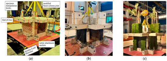
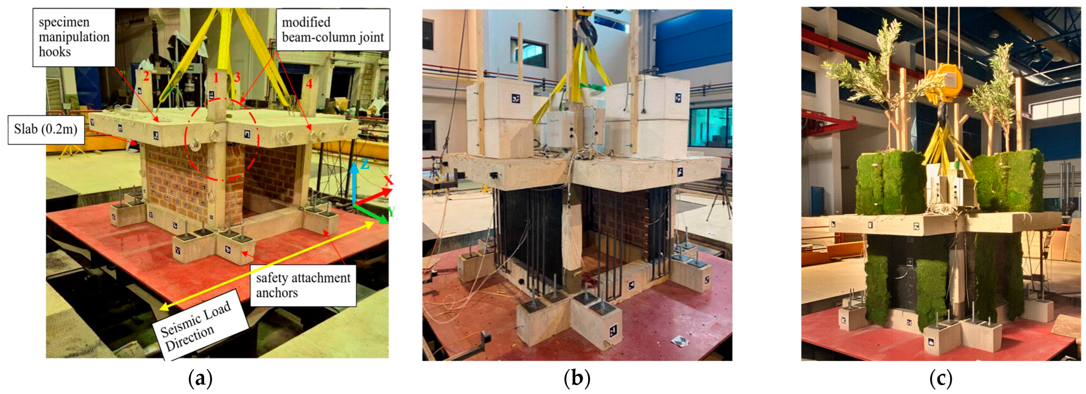
In the direction of seismic excitation, the specimen was configured with partial infill; in the perpendicular direction, the frame openings were filled with full infill. The interface between the concrete and the infill was grouted with standard mortar. The final configuration for Phase A is depicted in Figure 1a.

Figure 1. GREENERGY project specimen during (a) Phase A, (b) Phase B and (c) project final demonstration.

During Phase B, the specimen was retrofitted to enhance performance without causing significant disruption to building functionality. Specific interventions included a dedicated seismic joint at the vertical interface between column and infill, basalt rope wrapping applied around columns and fiber-reinforced jackets installed over the infill walls. In addition to seismic upgrades, the specimen received greenery enhancements in the form of eight vertical living wall panels—two on each façade—and five plant pods mounted on top of the slab, simulating the integration of vertical forest inside and outside the building envelope.

For further technical information regarding the selection criteria and methodology, please refer to [7]. The retrofitted configuration is illustrated in Figure 1b and the fully assembled specimen is shown in Figure 1c.

The specimen during Phase A and Phase B shared a common sensor layout (for technical specifications, please see published paper [7]):

• 12 uniaxial accelerometers, configured in groups of three to precisely capture acceleration in the X, Y, and Z global directions. Two groups were placed on the left and right sides of the slab extension’s median plane, one in the middle of the full infill and one at the mid-height of the foundation beam.
• 4 draw-wire sensors to measure displacement in the direction of seismic excitation. Two were positioned at the slab’s mid-height and two others at the mid-height of the foundation beams.
• 16 strain gauges to measure strain in the longitudinal rebars, and 4 surface-mounted strain gauges on the partial infills to monitor horizontal and vertical strains.
• 48 piezoelectric sensors (PZTs) to capture the specimen’s state after each loading sequence. Of these, 37 PZTs were embedded as “smart aggregates” within the structure (columns, slab, cantilevers), while 11 were externally bonded to the masonry infill surfaces.
• Unique ArUco markers for contactless displacement measurements.

During Phase B, 13 additional PZT sensors were installed to monitor the FRP jackets, basalt rope confinement and polyurethane joints. Furthermore, optical markers were added to the plant pods and the simulated tree extensions to obtain sub-millimeter in-plane displacement results in real-time for the entire duration of the seismic excitations (see [22] for proof of concept). The experimental methodology implemented herein—specifically the dense, multi-tiered sensor deployment and the use of sequential, incremental shake table protocols interspersed with diagnostic pauses—aligns with rigorous, state-of-the-art frameworks recently established for evaluating the dynamic resilience and component-level behavior of large-scale structural systems [23].

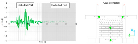
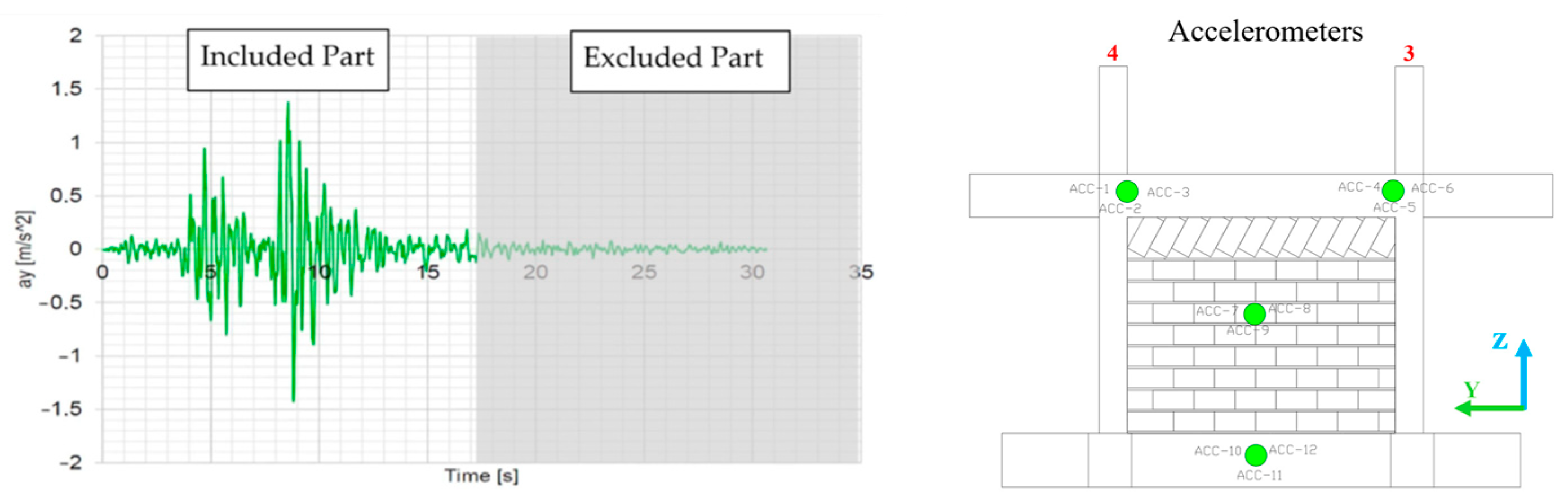
The experimental program consists of a dynamic pushover approach, incorporating 28 dynamic loads (comprising 14 white noise and 14 scaled seismic excitations based on the 1978 Thessaloniki earthquake record). To accurately capture the severity of the seismic demand, the actual input motions and Peak Ground Acceleration (PGA) at the base of the structure were continuously recorded by a dedicated triaxial accelerometer cluster (ACC-10, ACC-11, and ACC-12) securely mounted at the center of the foundation beam (see Figure 2). Comprehensive details regarding the exact input motions and multiple outputs for all 28 seismic excitations (other than optical monitoring) are documented in structural performance papers of the experimental campaign [6,7].

Figure 2. Reference seismic excitation used for all earthquake phases and triaxial accelerometer cluster (ACC-10 (X-direction), ACC-11 (Y-direction), and ACC-12 (Z-direction)) for input motion and PGA continue recording.

2.1. Primary Objectives

The primary objective of this study is to provide newly measured information, beyond the GREENERGY project [6,7], focusing herein on optical and measured permanent deformation detection of the structure and the greenery using a high-precision terrestrial LiDAR system. Specifically, the spatial positions of the five pods were investigated after repeated seismic excitations, along with the efficiency of the anchoring system at each stage. Moreover, the behavior of the critical fixing point at the bottom of the simulated living wall system was investigated alongside the orientation of each part. Finally, the spatial comparison of the entire reinforced concrete structure was investigated across different stages. Two point cloud densities were investigated: 100% (original) and a 5% random sample. The detailed methodology is provided in the following paragraphs.

2.2. LiDAR Information

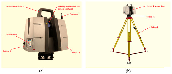
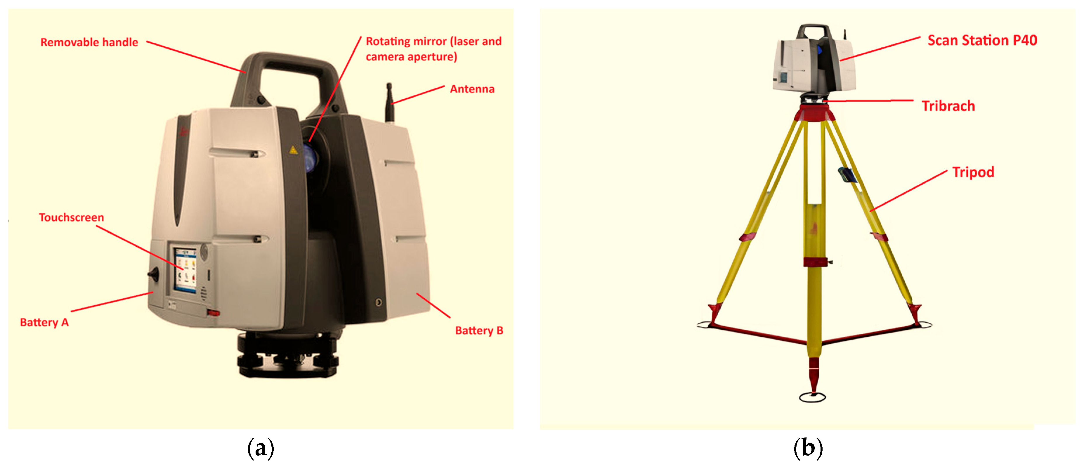
In the current study, the Leica Scan Station P40 (see Figure 3)—a high-precision terrestrial laser scanner (TLS) designed for demanding applications in cultural heritage documentation, archaeology and 3D geospatial analysis—was used. The current model offers survey-grade accuracy of 3 mm at 50 m and a robust operating temperature range (−20 °C to +50 °C), ensuring reproducible data essential for conservation studies where millimeter-level detail impacts interpretation. It supports an operational range of up to 270 m at 34% reflectivity, with real-time dual-axis tilt compensation critical for scanning uneven terrain. For imaging capture, it provides High-Dynamic Range (HDR) capability to enhance contextual analysis of material textures.

Figure 3. Leica TLS (a) Scan Station P40 details and (b) operational ready equipment after Tripod setup.

2.3. LiDAR Scanning Procedure

For the current analysis, three distinct phases of the specimen’s condition were recorded. The initial state, representing the reference virgin (undamaged) condition prior to any seismic excitation, served as the baseline for comparison. This was followed by the post-Phase A stage, during which the unretrofitted specimen underwent testing at the Serviceability Limit State (SLS). Finally, the terminal phase, captured at the conclusion of Phase B, documented the specimen after structural testing with vertical steel elements simulating soil and vegetation mass, alongside dual concrete pods equipped with extended wood components to replicate forest-structural elements and their interaction with the specimen.

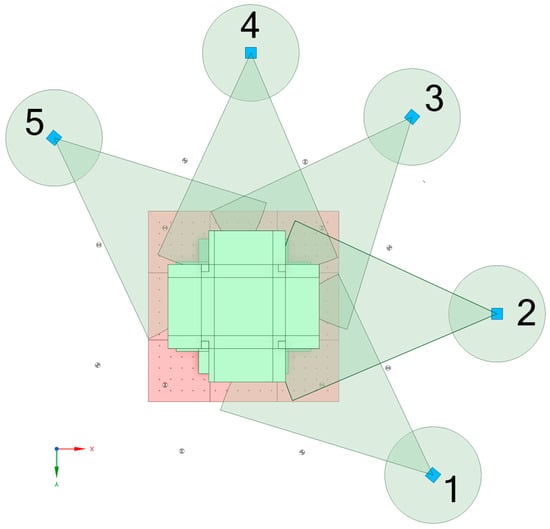
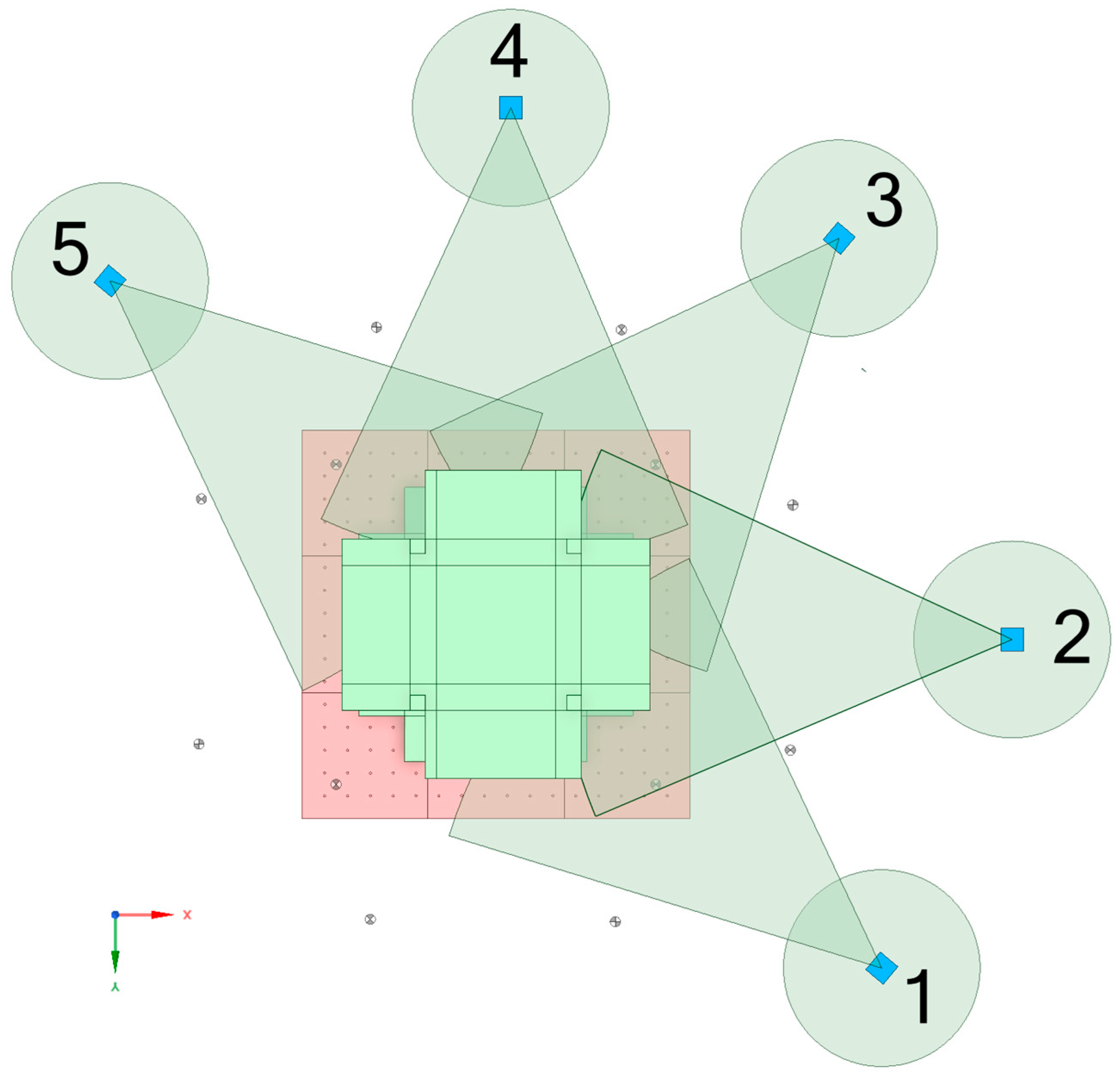
In all stages (except initial, 2–3–4), five scan positions were utilized, as indicated in Figure 4. The scanning procedure consisted of three scans at approximately 45-degree angles (relative to the direction of seismic excitation) and two direct scans parallel to the infills containing the ArUco markers. The scanning sequence followed a counter-clockwise direction, starting from Position 1 through Position 5. This strategy ensured adequate data density, both for the accurate registration of the generated point clouds and for capturing the critical geometry intended for comparison.

Figure 4. TLS scan position scheme and setup orientation.

Because TLS is inherently a static measurement tool requiring several minutes per scan position, all scanning procedures were conducted while the shake table was completely stationary, during scheduled pauses between the major experimental phases. Consequently, the generated point clouds exclusively capture the permanent, residual deformations (e.g., sliding, rotation, and plastic drift) of the structure and VGS components, complementing the real-time dynamic transient measurements captured by the continuous tracking systems.

All scanning was conducted using the settings described in Table 1.

Table 1. Laser scanning parameters and instrument configuration.

Property	Value	Description
Resolution	1.0 mm@5 m	Specifies the point spacing density at a 5-m radial distance.
Dual-Axis Compensator	ON	Ensures verticality and levels the instrument automatically during data acquisition.
Sensitivity	Normal	Balances scan speed and the quality of signal return from various surfaces.
EDM Mode	Speed	Optimizes the Electronic Distance Measurement for rapid data collection.
HDR Mode	ON	Enables High Dynamic Range imaging for improved texture mapping and visual clarity.

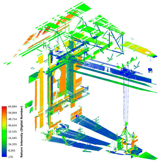
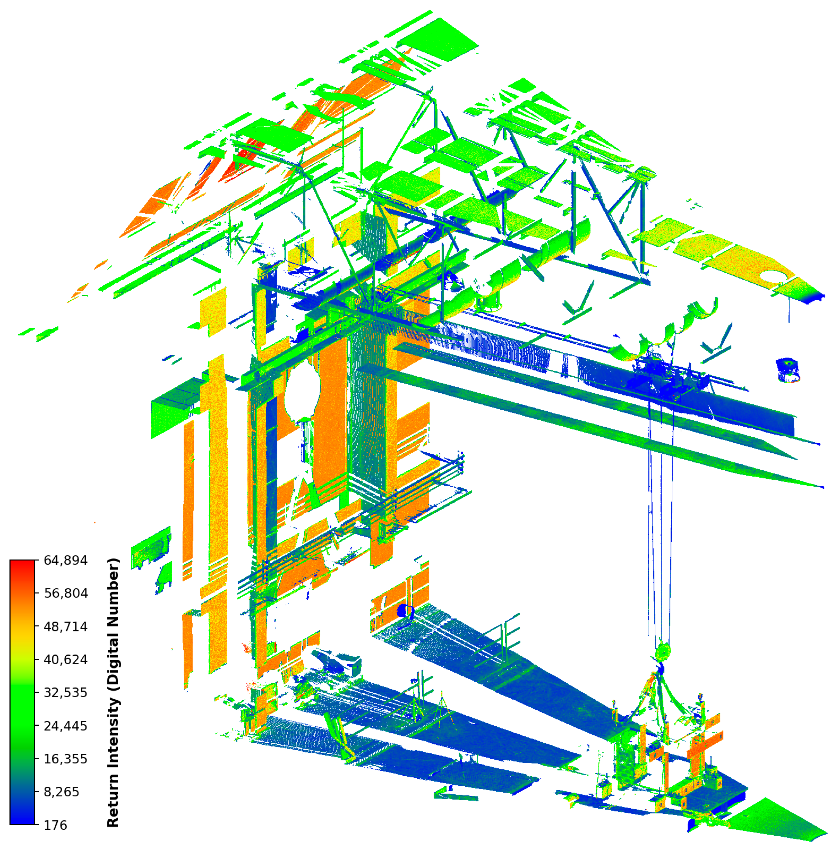
The average height of the Terrestrial Laser Scanner (TLS) was approximately 1.67 m. Figure 5 presents a raw scan obtained at the end of Phase A. During scanning, no distance restrictions were applied; consequently, the default 270 m range was automatically utilized. This approach ensured that many surrounding parts of the laboratory were also captured, which served as reference points for registration following the alignment of the scans.

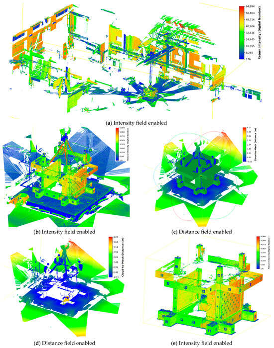
Figure 5. A raw scan from the end of Phase A (Intensity field enabled). The colors represent the relative laser return intensity, recorded as 16-bit dimensionless scalar values. The color scale ranges from blue (representing weak signal returns, min value ~176) through green and yellow, up to orange/red (representing strong signal returns, max value ~64,894).

It is critical to note that no automatic registration was applied initially. However, during the final stage—following manual alignment—an optimization algorithm [24,25,26,27,28] available in the CloudCompare v2.13.2 software was employed to enhance the results. To optimize data acquisition time and exclude irrelevant structural elements of the laboratory ceiling, the vertical scanning range was generally restricted between −55° and +14°. However, for scanner setups positioned directly adjacent to the specimen, the upper limit was extended to +90° to ensure the full geometry of the rooftop planter pods and simulated tree extensions were captured. The horizontal view was configured to encompass the entire structure, with a margin allowing for a slightly wider field of view from left to right to ensure a safe scanning procedure. As the laboratory floor exhibited no significant global Z-axis deviations, minimal leveling adjustments were required after the initial instrument alignment to ensure subsequent scanning points were perfectly aligned.

2.4. LiDAR Data Processing

The data captured by the TLS initially required processing with specific proprietary software. To ensure open availability for the research community, the data was subsequently converted to the .LAS format. All further processing was conducted using open-source software that supports both a Graphical User Interface (GUI) and Python API programming (CloudCompare v2.13.2 [29]).

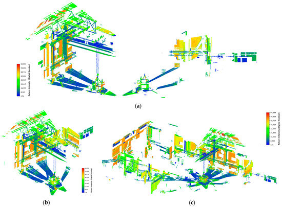
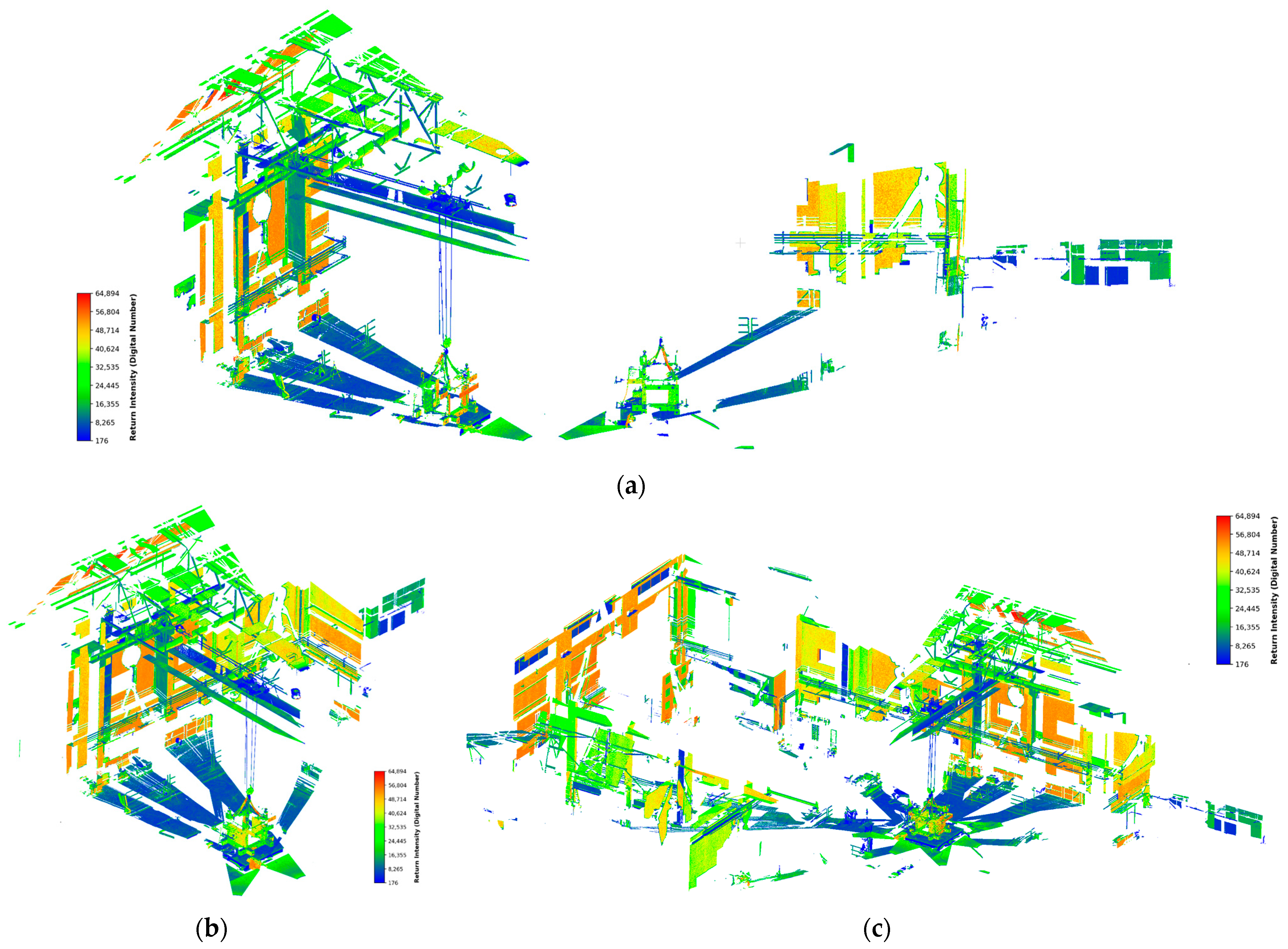
The initial data were manually aligned using translation and rotation tools, primarily focusing on the Global X and Global Y axes displacement, as the Global Z axis was already properly aligned. Rotation around the Global Z axis was performed only to position the scan at a logical distance for the final registration process. In point cloud terminology, “registration” refers to combining two different point cloud sources containing overlapping portions into a new, merged point cloud. The alignment process was identified to be more efficient when prioritizing the primary object of study (in this case, the experimental specimen) before aligning distant related objects. This method assisted in correcting Z-axis rotation, thereby minimizing final registration error. A demonstration of this process is depicted in Figure 6.

Figure 6. Point cloud data from end Phase A (Intensity field enabled) (a) raw scanning of position 2 (left) and 1 (right), (b) after manual adjustment then registration and (c) final registration process.

The object comparison experiment was conducted using two data densities: the original density and 1/20 of the original density. Furthermore, critical regions of interest (ROIs), such as pod and vertical living wall simulators, slab and columns were determined for later use.

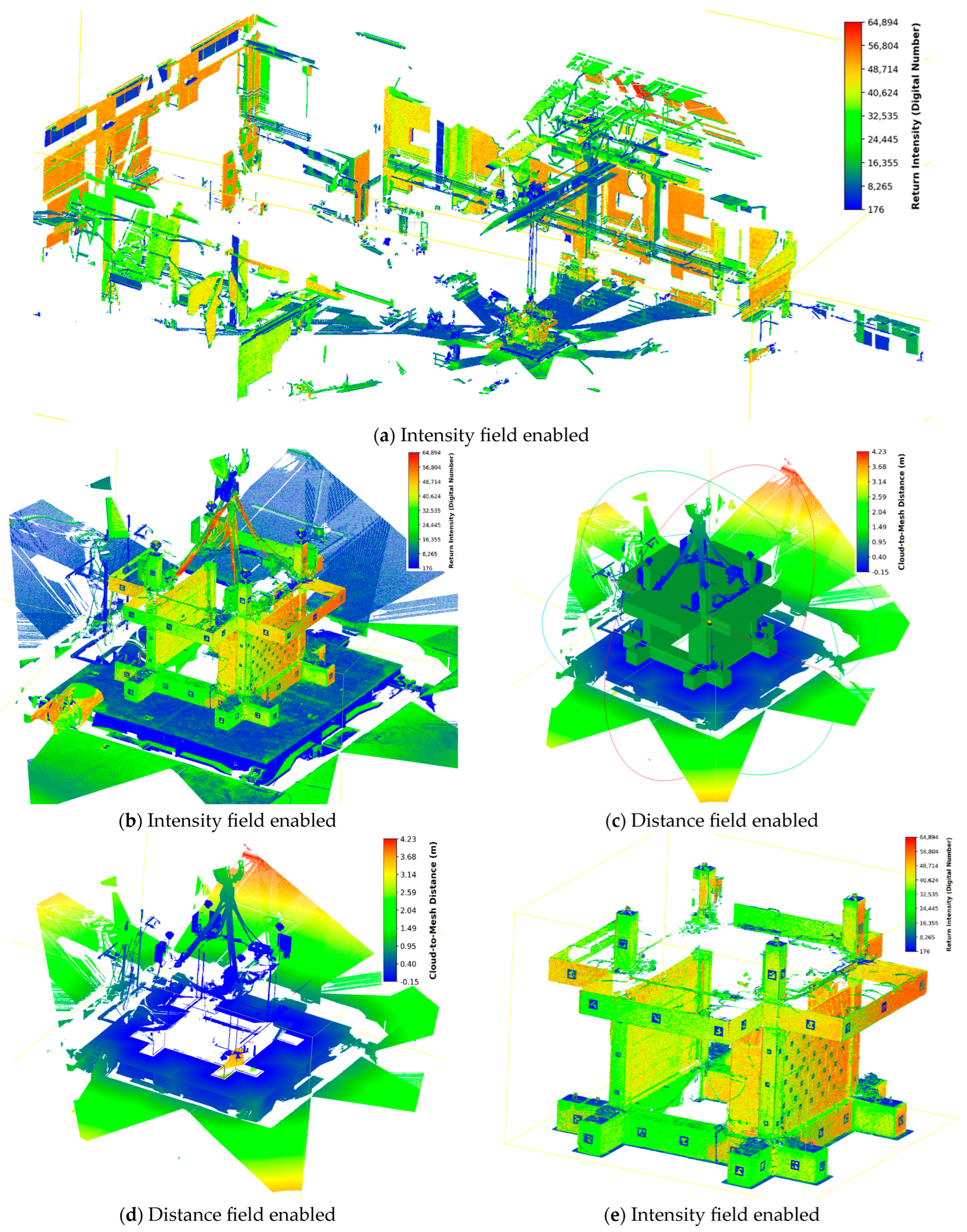
After an initial comparison, it became evident that objects introduced to the laboratory environment after the baseline scan increased the data field for distance comparison. The comparison algorithm identified these new objects as high scalar values, necessitating a cleaning process (outlined in Figure 7). Initially, the scene was isolated near the specimen area using a coarse crop of the original point cloud. A PointCloud to Mesh distance tool was used to clip the original point cloud using a 3D mesh from a previous Finite Element Method (FEM) simulation [30]. The 3D mesh was pulled out about 30 mm in all faces. This scaling provided adequate spacing for the algorithm to perform proper trimming while retaining data related to potential small, permanent deformations of the specimen.

Figure 7. Point cloud data cleaning process from (a) initial raw data, continuing to (b) coarse crop around the specimen region, (c) importing the FEM expanded geometry for proper boundary and implementing PointCloud to Mesh distance calculation, (d) exporting the outside field values (>0) and finally (e) exporting the inside data field (<0) with some overlapping of 0.015 m.

Following this process, any residual points not required for comparison were removed using polygon selection or RGB color filtering (with a ±1% deviation tolerance). To avoid the accidental removal of points within the desired region, the ROI was initially coarsely separated from the scene. The polygon selection or color removal filter was then applied to the background data before merging the datasets back together.

To quantitatively evaluate the accuracy of this final registration, the Root Mean Square (RMS) alignment error was calculated following the Iterative Closest Point (ICP) optimization. By utilizing the stable, non-deforming elements of the laboratory environment (such as the floor and the robust foundation system) as reference geometries, the fine registration achieved a final RMS error of 0.00174 m. This low alignment error confirms a highly accurate geometric registration, ensuring that subsequent displacement calculations are not artifacts of scan misalignment.

While Cloud-to-Cloud (C2C) scalar fields provide global displacement magnitudes, they do not inherently resolve specific directional vectors or rotational angles for individual components. To extract precise kinematic parameters for the VGS elements a manual feature-based measurement approach was utilized using CloudCompare.

• Translation: Distinct, geometrically stable corners of each pod were identified in both the reference and deformed point clouds. The “Measure Distance” tool was used to select these two corresponding points, calculating the Euclidean distance between them to determine the net translation.
• Rotation: To calculate rotational displacement, three non-collinear geometric features (corners or edges) were selected on each component in both scans. Using the “Measure Angle” tool, the angle formed by the vectors connecting these three points was computed relative to the reference orientation. This method allows for the precise determination of rotation angles based on the rigid movement of specific geometric features.

3. Results and Discussion

Scanning results were compared across four stages—S1 (Initial state), S2 (Post-Phase A), S3 (Pre-Phase B), and S4 (Post-Phase B)—to evaluate permanent global and potential local column deformations as follows:

S1 vs. S2: To analyze the effects of Phase A.

S3 vs. S4: To assess the impact of Phase B.

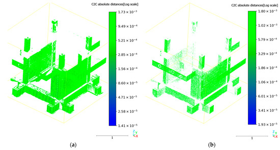
S1 vs. S4: To determine the cumulative results of the entire experimental event. The comparison results for the initial state and final stage after Phase A (S1 vs. S2) are depicted in Figure 8. The contact analysis sensors of the experimental setups, draw-wires sensors recorded a permanent displacement of 0.25 mm at the end of the Phase A. The LiDAR analysis provides adequate average range for measurement correlation. As shown in the legend in Figure 8a, the majority of the specimen surfaces are rendered in the green spectrum, corresponding to values from 1.0 × 10⁻⁴ m and 5.0 × 10⁻⁴ m. The maximum scalar values recorded in the scale bar (≈1.7 mm) represent noise at the edges rather than structural drift. This value (≈1.7 mm) effectively establishes the spatial uncertainty bound (noise floor) for the methodology, encompassing both inherent scanner ranging error and ICP (Iterative Closest Point) registration error. Displacements must exceed this threshold to be confidently distinguished from registration noise. The point cloud successfully captures the elastic behavior of the specimen, confirming that no significant permanent deformation occurred during Phase A.

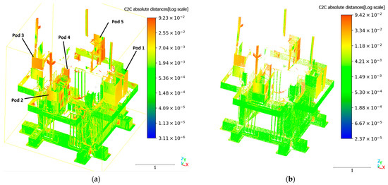
Figure 8. Comparison of S1 vs. S2 using cloud-to-cloud distance (absolute distance field enabled) for (a) 100% and (b) 5% (random) point cloud data.

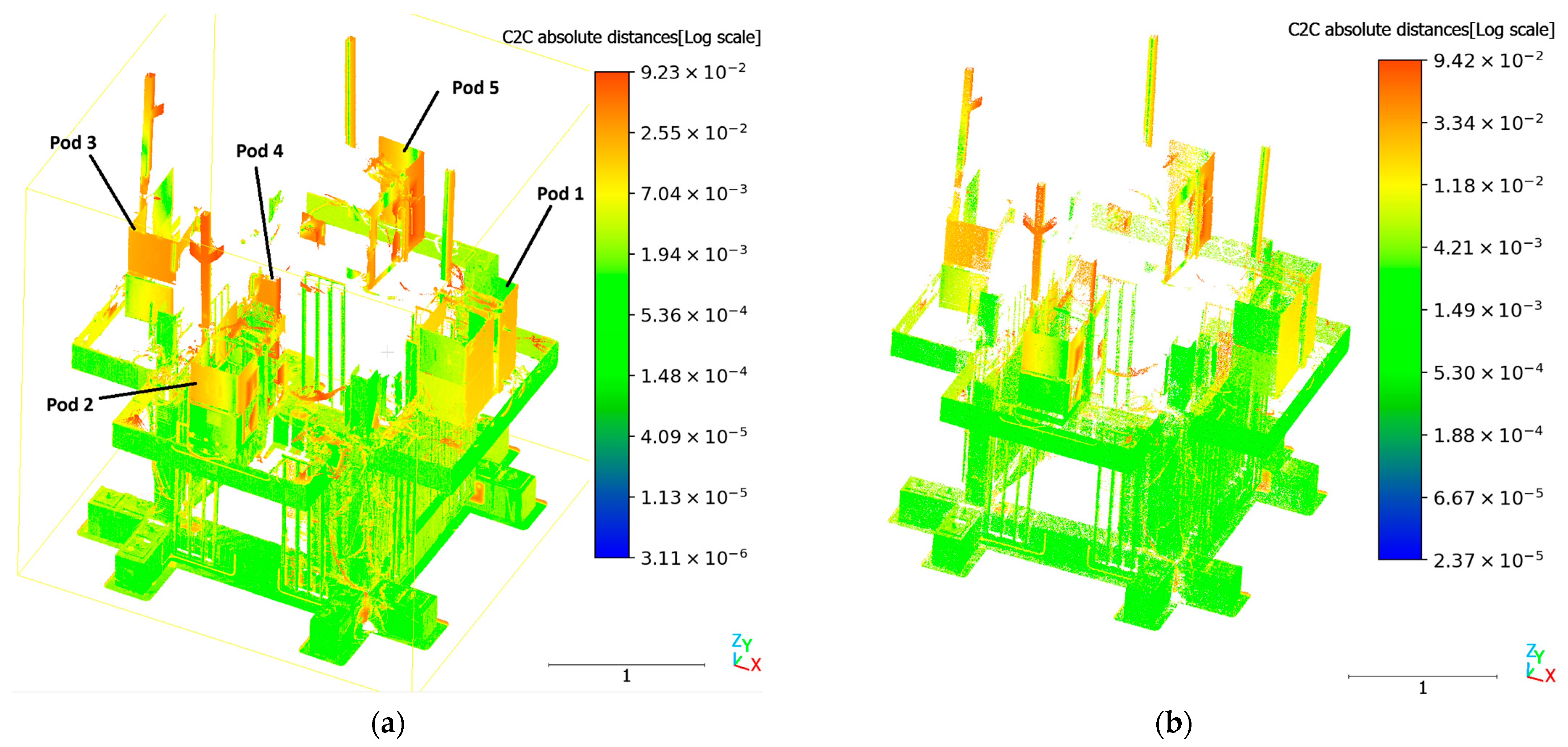
Following the intense repeated (28) seismic excitations Phase B ended. The initial and final result comparison is provided in Figure 9a, where the draw-wire sensors recorded 2.37 mm of permanent structural displacement. The slab region of the specimen remains under 2.0 × 10⁻³ m in the scalar field. This confirms that the terrestrial laser scanner can reliably detect permanent drifts in the millimeter range, matching the precision of dedicated displacement sensors.

Figure 9. Comparison of S3 vs. S4 using cloud-to-cloud distance (absolute distance field enabled) for (a) 100% and (b) 5% (random) point cloud data.

A significant advantage of the LiDAR implementation was the ability to capture the behavior of the vertical greenery elements, which were difficult to monitor via the installed draw-wire sensors. Figure 9 highlights a significant displacement deviation in the upper region of the specimen during Phase B.

While the reinforced concrete frame remained within safe displacement limits, the simulated planter pods exhibited distinct independent movements based on their anchoring configuration [7]. The most critical behavior was observed in the middle planter (Pod 4), visible as the orange/red element in Figure 9. The scalar field indicates a maximum displacement value of approximately 9.2 cm (9.2 × 10⁻² m) at the tips. Detailed analysis of the point cloud coordinates reveals that Pod 4 experienced a net translational displacement of approximately 8 cm relative to the excitation direction. This excessive movement is directly attributed to its anchoring configuration (Configuration 4); this pod lacked mechanical fastening (fiber or steel) and relied solely on friction provided by polyurethane sheets placed between the pod and the concrete slab. The repetitive seismic energy introduced during Phase B evidently overcame the friction resistance, leading to significant sliding.

This excessive movement can be quantitatively validated by comparing the expected seismic inertial demand against the available sliding resistance. Planter 4 (Configuration 4) relied entirely on the friction provided by Polyurethane PM pads. The total mass of the planter assembly was $\mathrm{m}=159 \mathrm{kg}$ (comprising the 153 kg concrete double-planter and 6 kg of simulated trees). Based on experimental material testing, the static friction coefficient for the polyurethane-concrete interface was determined to be $\mathsf{\mu }\approx 0.70$. For the polyurethane-concrete interface, the effective sliding resistance is calculated as ${\mathrm{V}}_{\mathrm{R}}=\mathsf{\mu }\cdot \mathrm{m}\cdot \mathrm{g}\approx 1.09 \mathrm{kN}$. According to the structural accelerometer data, the Peak Floor Acceleration (PFA) at the slab level during the maximum EQ1.4 g excitation reached 1.8 g. This generated a peak seismic inertial demand of ${\mathrm{F}}_{\mathrm{I}}=\mathrm{m}\cdot \mathrm{PFA}\approx 2.81 \mathrm{kN}$. Because the maximum inertial demand ($2.81 \mathrm{kN}$) exceeded the frictional resistance ($1.09 \mathrm{kN}$) by a factor of approximately 2.6, severe sliding was mechanically inevitable. Furthermore, the theoretical acceleration threshold required to initiate sliding (${\mathrm{a}}_{slide}=\mathsf{\mu }\cdot \mathrm{g}\approx 0.70 \mathrm{g}$) was first exceeded during the EQ0.5 g excitation stage (where the recorded PFA reached $0.77 \mathrm{g}$). This mathematical threshold perfectly correlates with experimental observations, as the first micro-displacements of Planter 4 were visually documented at exactly EQ0.5 g, ultimately culminating in the cumulative ≈8 cm sliding captured by the TLS.

In contrast, the pods equipped with mechanical anchoring (Pods 1, 2, 3, and 5) exhibited different kinematic behaviors, primarily characterized by rotation rather than pure translation:

• Pod 1 (anchored with a steel rod, Configuration 1) exhibited the stiffest response, recording a limited translational displacement of 1.3 cm in the X-direction.
• Pods 2, 3, and 5, which were anchored using basalt rope tendons (Configurations 2, 3, and 5, respectively), experienced significant rotation around the vertical Z-axis (yawing) rather than global sliding.
• Pod 5 (two fully post-tensioned basalt ropes) experienced the most severe rotation of −13.09° about the Z-axis.
• Pod 2 (one fully tensioned, one partial basalt rope) experienced a rotation of −4.44° about the Z-axis.
• Pod 3 (one fully tensioned, one partial basalt rope) recorded a rotation of +1.82° about the Z-axis, combined with a 2.78 cm slide of the top and bottom sub-pods along the Y-axis.

Additionally, the simulated tree elements extending from Pods 2, 3, and 5 showed an average top displacement of 6.3 cm, indicating a whipping effect at the canopy level despite the base anchoring.

Finally, regarding the vertical living wall panels on the façade, no significant centimeter-magnitude displacement or rotation was observed. This stability indicates that the metal anchoring system provided for the vertical living wall was adequate to overcome the repetitive inertial energy introduced during Phase B.

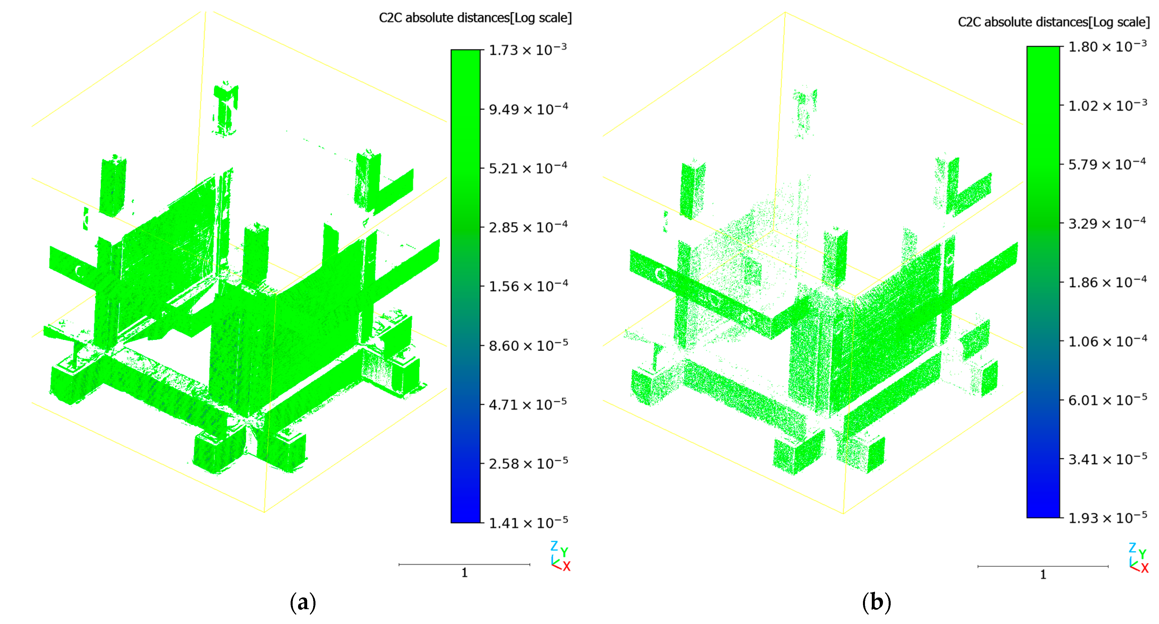
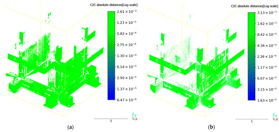
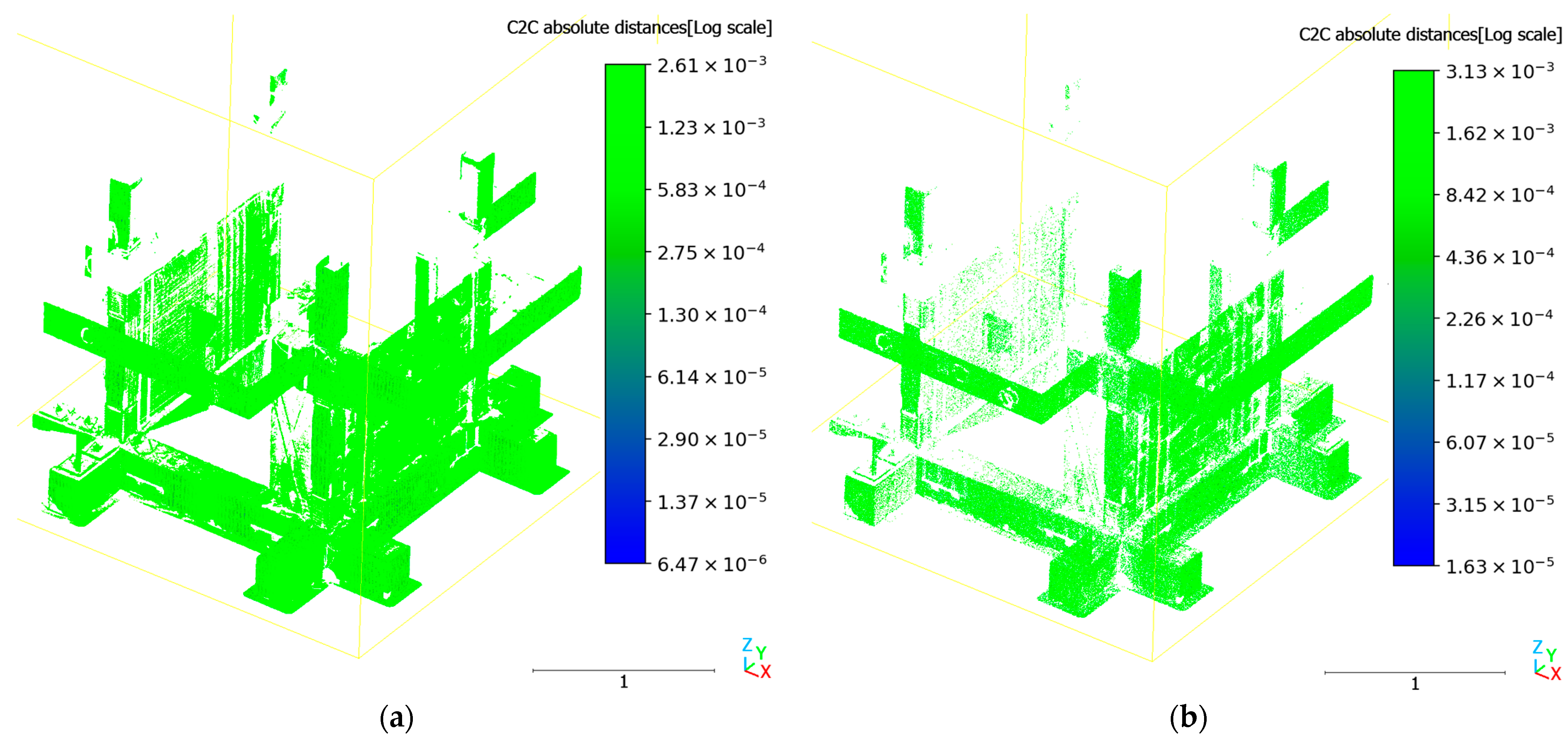
To isolate the structural performance without the visual obstruction of the greenery displacements, a comparison of the structural common components between Phase A and Phase B is provided in Figure 10.

Figure 10. Comparison of S1 vs. S4 using cloud-to-cloud distance (absolute distance field enabled) for (a) 100% and (b) 5% (random) point cloud data.

To validate the feasibility of using lighter data payloads (e.g., for drone-based inspection or rapid processing), the results from the full-resolution scans (100% density, ≈80 million points) were compared against a random subsample of 5% (≈ 4 million points). Visual inspection of Figure 8, Figure 9 and Figure 10 reveals that the deformation patterns are identical. The spatial distribution of the scalar fields is perfectly preserved in the lower density clouds. To quantify the difference, the maximum scalar values recorded in the legends were compared:

• Phase A (Figure 8): The maximum range deviated slightly (1.73 mm for 100% vs. 1.80 mm for 5%), a negligible absolute difference of 0.07 mm.
• Phase B (Figure 9): The critical high-deformation zones showed high consistency, with maximum recorded values of 92.3 mm (100%) and 94.2 mm (5%).
• Relative Difference: across all stages, the relative difference between the dense and sparse point clouds in quantifying peak displacement was found to be approximately 2%.
• To rigorously quantify the reliability of the density reduction, a point-to-point statistical comparison was performed between the scalar fields of the full-resolution (100%) and subsampled (5%) point clouds. The difference field between the two datasets exhibited a mean deviation of −1.13 mm and a standard deviation of 2.81 mm. This results in a global Root Mean Square Error (RMSE) of 3.03 mm across the entire structural envelope. Given that the critical high-deformation zones (such as the planter pods) exhibited maximum displacements of up to 94.2 mm, this low RMSE demonstrates that the spatial distribution and magnitude of the deformations are statistically preserved. Given that the global deviation is minimal and the relative percentage difference is significantly low, it is concluded that a 5% sampling density is sufficient for detecting both global drift and local component failures. This reduction allows for processing speeds up to 20 times faster without compromising diagnostic accuracy.

Beyond the structural assessment presented herein, this study’s findings highlight the broader applicability of high-precision TLS in geotechnical monitoring. The accurate detection of millimetric permanent drift, rotational behavior, and friction-controlled sliding mechanisms demonstrates the capability of point cloud comparison techniques to capture soil–structure interaction effects and cyclic displacement accumulation. Similar methodologies may be extended to geotechnical systems such as shallow foundations, retaining structures, and rockfall-prone slopes, where early identification of localized displacement or detachment zones is critical for risk mitigation. The demonstrated reliability of reduced-density datasets (5% sampling) further supports the feasibility of rapid field deployment, including drone-based TLS surveys for large-scale slope and rock mass stability assessments.

4. Conclusions

The current study investigates the use of a high-precision terrestrial laser scanner for permanent deformation detection on a typical old structure that has undergone simulated seismic and greenery/energy upgrading. It provides a reliable pipeline for scanning and processing large amounts of point cloud data (80 million points and above per scan) on a regular mid-to-high-end computer system. Furthermore, it offers a quick identification system for elements that were introduced or excluded from the examined system using open-source technology. The comparison with the experimental draw-wire equipment for permanent deformation is quite close, while additionally providing displacement details for nearly the entire envelope. It has been proven that the algorithm can provide adequate information using only one-twentieth (5%) of the original data; this could lead to practically real-time applications when scanning is conducted from a drone equipped with similar capabilities. The primary limitation of this application is that prior scanning data of the structure is required. Generally, the data from the current study indicate that the vertical forest pod supporting system is more affected by sequential severe seismic events, in terms of permanent point-to-point displacement than a living vertical wall supporting system. Crucially, this work builds upon previous TLS-based monitoring studies by demonstrating the capability to isolate differential kinematic behaviors (sliding, rotation) within VGS components. By leveraging high-resolution 3D point clouds, the study captures localized deformation patterns across the component surface, providing enhanced spatial detail that complements conventional instrumentation and supports a more granular assessment of structural stability. TLS may provide a rapid and reliable performance-based assessment of the whole system to allow for holistic decision making during emergency situations.

References

- Besir, A.B.; Cuce, E. Green Roofs and Facades: A Comprehensive Review. Renew. Sustain. Energy Rev. 2018, 82, 915–939. [Google Scholar] [CrossRef] [Scilit]
- Manso, M.; Castro-Gomes, J. Green Wall Systems: A Review of Their Characteristics. Renew. Sustain. Energy Rev. 2015, 41, 863–871. [Google Scholar] [CrossRef] [Scilit]
- Pérez, G.; Rincón, L.; Vila, A.; González, J.M.; Cabeza, L.F. Green Vertical Systems for Buildings as Passive Systems for Energy Savings. Appl. Energy 2011, 88, 4854–4859. [Google Scholar] [CrossRef] [Scilit]
- Manouchehri, M.; Santiago López, J.; Valiente López, M. Sustainable Design of Vertical Greenery Systems: A Comprehensive Framework. Sustainability 2024, 16, 3249. [Google Scholar] [CrossRef] [Scilit]
- Vanian, V.; Fanaradelli, T.; Rousakis, T. A Comprehensive Review of Vertical Forest Buildings: Integrating Structural, Energy, Forestry, and Occupant Comfort Aspects in Renovation Modeling. Fibers 2025, 13, 101. [Google Scholar] [CrossRef] [Scilit]
- Rousakis, T.; Vanian, V.; Lappa, M.; Zapris, A.G.; Xynopoulos, I.P.; Voutetaki, M.; Kellis, S.; Sapidis, G.; Naoum, M.; Papadopoulos, N.; et al. Experimental Evaluation of RC Structures with Brick Infills for Vertical Forest Adaptation in Seismic Regions. Fibers 2025, 13, 154. [Google Scholar] [CrossRef] [Scilit]
- Rousakis, T.; Vanian, V.; Lappa, M.; Zapris, A.G.; Xynopoulos, I.P.; Voutetaki, M.E.; Kellis, S.; Sapidis, G.M.; Naoum, M.C.; Papadopoulos, N.A.; et al. Assessment of Seismic Performance and Structural Health Monitoring of a Retrofitted Reinforced Concrete Structure with Polyurethane-Based Interventions and Vertical Greenery Systems. Polymers 2025, 17, 3104. [Google Scholar] [CrossRef] [Scilit]
- Teng, J.; Shi, Y.; Wang, H.; Wu, J. Review on the Research and Applications of TLS in Ground Surface and Constructions Deformation Monitoring. Sensors 2022, 22, 9179. [Google Scholar] [CrossRef] [Scilit]
- Shen, N.; Wang, B.; Ma, H.; Zhao, X.; Zhou, Y.; Zhang, Z.; Xu, J. A Review of Terrestrial Laser Scanning (TLS)-Based Technologies for Deformation Monitoring in Engineering. Measurement 2023, 223, 113684. [Google Scholar] [CrossRef] [Scilit]
- Olsen, M.J.; Kuester, F.; Chang, B.J.; Hutchinson, T.C. Terrestrial Laser Scanning-Based Structural Damage Assessment. J. Comput. Civ. Eng. 2010, 24, 264–272. [Google Scholar] [CrossRef] [Scilit]
- Mosalam, K.M.; Takhirov, S.M.; Park, S. Applications of Laser Scanning to Structures in Laboratory Tests and Field Surveys. Struct. Control Health Monit. 2014, 21, 115–134. [Google Scholar] [CrossRef] [Scilit]
- Pesci, A.; Teza, G.; Bonali, E.; Casula, G.; Boschi, E. A Laser Scanning-Based Method for Fast Estimation of Seismic-Induced Building Deformations. ISPRS J. Photogramm. Remote Sens. 2013, 79, 185–198. [Google Scholar] [CrossRef] [Scilit]
- Aubertin, J.D.; Hutchinson, D.J. Scale-Dependent Rock Surface Characterization Using LiDAR Surveys. Eng. Geol. 2022, 301, 106614. [Google Scholar] [CrossRef] [Scilit]
- Teza, G.; Pesci, A.; Genevois, R.; Galgaro, A. Characterization of Landslide Ground Surface Kinematics from Terrestrial Laser Scanning and Strain Field Computation. Geomorphology 2008, 97, 424–437. [Google Scholar] [CrossRef] [Scilit]
- Seo, H. Long-Term Monitoring of Zigzag-Shaped Concrete Panel in Retaining Structure Using Laser Scanning and Analysis of Influencing Factors. Opt. Lasers Eng. 2021, 139, 106498. [Google Scholar] [CrossRef] [Scilit]
- Dunning, S.A.; Massey, C.I.; Rosser, N.J. Structural and Geomorphological Features of Landslides in the Bhutan Himalaya Derived from Terrestrial Laser Scanning. Geomorphology 2009, 103, 17–29. [Google Scholar] [CrossRef] [Scilit]
- Wang, M.; Zhou, J.; Chen, J.; Jiang, N.; Zhang, P.; Li, H. Automatic Identification of Rock Discontinuity and Stability Analysis of Tunnel Rock Blocks Using Terrestrial Laser Scanning. J. Rock Mech. Geotech. Eng. 2023, 15, 1810–1825. [Google Scholar] [CrossRef] [Scilit]
- Marinos, V.; Prountzopoulos, G.; Asteriou, P.; Papathanassiou, G.; Kaklis, T.; Pantazis, G.; Lambrou, E.; Grendas, N.; Karantanellis, E.; Pavlides, S. Beyond the Boundaries of Feasible Engineering Geological Solutions: Stability Considerations of the Spectacular Red Beach Cliffs on Santorini Island, Greece. Env. Earth Sci 2017, 76, 513. [Google Scholar] [CrossRef] [Scilit]
- Farmakis, I.; DiFrancesco, P.-M.; Hutchinson, D.J.; Vlachopoulos, N. Rockfall Detection Using LiDAR and Deep Learning. Eng. Geol. 2022, 309, 106836. [Google Scholar] [CrossRef] [Scilit]
- Letortu, P.; Costa, S.; Maquaire, O.; Delacourt, C.; Augereau, E.; Davidson, R.; Suanez, S.; Nabucet, J. Retreat Rates, Modalities and Agents Responsible for Erosion along the Coastal Chalk Cliffs of Upper Normandy: The Contribution of Terrestrial Laser Scanning. Geomorphology 2015, 245, 3–14. [Google Scholar] [CrossRef] [Scilit]
- Abellán, A.; Jaboyedoff, M.; Oppikofer, T.; Vilaplana, J.M. Detection of Millimetric Deformation Using a Terrestrial Laser Scanner: Experiment and Application to a Rockfall Event. Nat. Hazards Earth Syst. Sci. 2009, 9, 365–372. [Google Scholar] [CrossRef] [Scilit]
- Vanian, V.; Rousakis, T.; Xynopoulos, I.; Kytinou, V.; Zapris, A.; Chalioris, C. Contactless Precise In-Plane Dynamic Displacement Measurements of Structures Using ArUco Markers. In Proceedings of the 6th Panhellenic Conference on Earthquake Engineering and Technical Seismology (6th PCEETS), Athens, Greece, 30 November 2025. [Google Scholar]
- He, X.; Chen, Y.; Zhou, Z.; Ke, K. Fuse Replacement Implementation by Shaking Table Tests on Hybrid Moment-Resisting Frame. J. Build. Eng. 2024, 95, 110232. [Google Scholar] [CrossRef] [Scilit]
- Pomerleau, F.; Colas, F.; Siegwart, R. A Review of Point Cloud Registration Algorithms for Mobile Robotics. Found. Trends Robot. 2015, 4, 1–104. [Google Scholar] [CrossRef] [Scilit]
- Rusinkiewicz, S.; Levoy, M. Efficient Variants of the ICP Algorithm. In Proceedings of the Third International Conference on 3-D Digital Imaging and Modeling, Quebec City, QC, Canada, 28 May–1 June 2001; pp. 145–152. [Google Scholar]
- Zhang, Z. Iterative Point Matching for Registration of Free-Form Curves and Surfaces. Int. J. Comput. Vis. 1994, 13, 119–152. [Google Scholar] [CrossRef] [Scilit]
- Besl, P.J.; McKay, N.D. A Method for Registration of 3-D Shapes. IEEE Trans. Pattern Anal. Mach. Intell. 1992, 14, 239–256. [Google Scholar] [CrossRef] [Scilit]
- Chen, Y.; Medioni, G. Object Modelling by Registration of Multiple Range Images. Image Vis. Comput. 1992, 10, 145–155. [Google Scholar] [CrossRef] [Scilit]
- CloudCompare Developers. CloudCompare Developers. CloudCompare, version 2.13.2; Lunaweb GmbH: Munich, Germany, 2024. [Google Scholar]
- Vanian, V.; Rousakis, T. FRESCO: An Open Database for Fiber and Polymer Strengthening of Infilled RC Frame Systems. Fibers 2025, 13, 152. [Google Scholar] [CrossRef] [Scilit]
Disclaimer/Publisher’s Note: The statements, opinions and data contained in all publications are solely those of the individual author(s) and contributor(s) and not of MDPI and/or the editor(s). MDPI and/or the editor(s) disclaim responsibility for any injury to people or property resulting from any ideas, methods, instructions or products referred to in the content. |
© 2026 by the authors. Licensee MDPI, Basel, Switzerland. This article is an open access article distributed under the terms and conditions of the Creative Commons Attribution (CC BY) license.