


Abstract
Accurate assessment of soil organic carbon (SOC) distribution is essential for carbon accounting and sustainable land management, yet spatial information remains limited in Central African landscapes. This study evaluated SOC stocks across cropland, grassland, and forest ecosystems in the Foumbot agricultural basin, western Cameroon, at depths of 0–10 and 10–20 cm. Spatial dependence was assessed using semivariograms, while a two-step, land use-based residual interpolation framework was applied. Land use-specific means were used to account for broad land use-related variation, and the resulting residuals were interpolated using Ordinary Kriging (OK) and Inverse Distance Weighting (IDW). Predictive performance was evaluated using leave-one-out cross-validation (LOOCV) and compared with direct interpolation and a mean per land use baseline. SOC stocks showed heterogeneity associated with land use, topography, and soil development. The fitted Gaussian semivariogram model described the spatial dependence of SOC stock residuals, with ranges of 167 and 144 m at 0–10 and 10–20 cm, respectively. At 0–10 cm, residual IDW achieved the lowest root mean square error (RMSE; 15.69 t ha−1), closely followed by residual OK (15.82 t ha−1), compared with direct IDW (19.60 t ha−1), direct OK (18.73 t ha−1), and the land use mean baseline (17.76 t ha−1). At 10–20 cm, residual OK performed best (RMSE = 14.28 t ha−1), closely followed by residual IDW (14.44 t ha−1), outperforming direct interpolation and the baseline. Overall, residual-based interpolation reduced prediction errors at both depths, although performance varied by depth and evaluation metric. These findings support its application in SOCS mapping and provide spatial information for targeted carbon management and sustainable soil management in tropical volcanic landscapes.
1. Introduction
Soil organic carbon (SOC) is a key component of soil quality and ecosystem functioning because it influences nutrient cycling, aggregate stability, water retention, biological activity, and carbon sequestration. Tropical regions are particularly important in the global carbon cycle because they contain substantial carbon reserves while experiencing rapid land use changes driven by agricultural expansion and population growth. However, tropical soils remain less documented than those of temperate regions, creating uncertainty in regional and global carbon assessments.
Land use change is one of the main factors controlling SOC dynamics. The conversion of forests and natural ecosystems into croplands and grasslands alters vegetation cover, organic matter inputs, root biomass, and decomposition processes, thereby influencing SOC storage and distribution. Previous studies have shown that forests generally maintain higher SOC stocks than cultivated lands, while grasslands and agroforestry systems often present intermediate levels depending on local environmental conditions and management practices [1,2]. Consequently, quantifying SOC stocks under contrasting land uses has become essential for understanding carbon dynamics and developing sustainable land management strategies.
The distribution of SOC is inherently heterogeneous because it reflects the combined influence of climate, vegetation, topography, parent material, soil-forming processes, and land use practices. These factors affect organic matter production, decomposition, stabilization, and redistribution, generating significant variations in SOC stocks over short distances. In agricultural landscapes, differences in tillage intensity, residue management, crop cover, and grazing pressure frequently create distinct patterns of carbon accumulation and depletion. Understanding this spatial variability is therefore crucial for identifying carbon-rich and carbon-poor zones, improving carbon inventories, and supporting site-specific management practices [1,3].
In Sub-Saharan Africa, information on SOC stocks remains limited despite the essential role of soils in supporting food security, ecosystem services, and climate change adaptation. In some regions of Cameroon, studies have reported differences in SOC stocks among land use types. Ref. [3] reported marked differences in SOC stocks among forests, agroforestry systems, savannas, and croplands in the forest–savanna transition zone, while [4] observed higher SOC stocks under natural vegetation than under cultivated lands in the Noun Plain of western Cameroon. These findings indicate that SOC distribution is strongly influenced by environmental conditions and management practices and highlight the need for local-scale assessments in major agricultural regions.
Foumbot, located in the Noun Plain of western Cameroon, is one of the country’s most important agricultural production areas because of its fertile volcanic soils and favorable climatic conditions. The landscape comprises croplands, grasslands, and remnant forest ecosystems that are increasingly affected by agricultural intensification. Recent pedological investigations by [5] revealed substantial variability in soil morphology, physicochemical properties, mineralogy, and classification along a climotoposequence. The study identified Andosols in upper landscape positions and Ferralsols in lower positions and reported significant variations in soil organic carbon content associated with topography and pedogenic processes. The authors also highlighted potential soil degradation risks linked to intensive land use and environmental variability, emphasizing the need for sustainable soil resource management.
Despite these advances, important knowledge gaps remain concerning the spatial distribution of SOC stocks within the Foumbot agricultural landscape. Existing studies have mainly focused on soil morphology, classification, mineralogy, physicochemical properties, or localized assessments of SOC [3,4,5]. However, little information is available on the spatial variability in SOC stocks across the dominant land use systems of Foumbot, namely cropland, grassland, and forest ecosystems. Furthermore, the performance of commonly used interpolation techniques for predicting SOC distribution has not yet been evaluated in this agricultural basin. This lack of information limits accurate estimation of SOC stocks and the identification of priority areas for carbon sequestration and sustainable land management.
Geostatistical approaches provide powerful tools for characterizing and mapping the spatial variability in soil properties. Ordinary Kriging (OK) is widely used because it incorporates spatial dependence through semivariogram modeling and provides unbiased predictions with associated estimation errors. Inverse Distance Weighting (IDW), in contrast, estimates unknown values using distance-weighted averages of neighboring observations. Since the performance of these methods depends on sampling density, spatial structure, and landscape heterogeneity, comparative evaluations are required to determine the most suitable approach for SOC mapping in each environment [6].
Previous studies in Africa have applied a range of spatial interpolation techniques to map SOC, including Ordinary Kriging (OK), Inverse Distance Weighting (IDW), radial basis functions, and regression kriging [7,8,9]. However, their relative performance has varied among study areas. For example, OK outperformed IDW for SOC mapping in Ethiopia [7,8], whereas IDW performed competitively with or better than kriging in other settings. More importantly, some studies have incorporated spatial interpolation of model residuals rather than directly interpolating SOC observations. In Cameroon, Ref. [10] combined machine learning models with both OK and IDW for residual interpolation of SOC stocks and found that the two approaches produced comparable performance. Similarly, regression kriging approaches have demonstrated improvements over regression-only models in Ghana and Kenya [9,11]. These findings suggest that interpolation performance is context-dependent and that accounting for systematic spatial trends before interpolating residuals may improve SOC prediction.
The novelty of this study is in integrating soil profile characterization with a two-step land use-based residual interpolation framework, to investigate the spatial variability in SOC stocks under contrasting land use systems in Foumbot. Unlike previous studies that focused primarily on soil classification, pedogenesis, mineralogy, or generalized SOC assessments [3,4,5], as well as studies relying on direct SOC interpolation [8,12], this study integrates field-based pedological observations with spatial modeling techniques. Specifically, we first characterize the land use-specific trends in SOC stocks using the mean SOC stock for each land use type and subsequently interpolate the residuals to quantify and map the spatial distribution of SOC stocks across cropland, grassland, and forest ecosystems. The predictive performance of the two-step residual interpolation framework is compared with that of direct interpolation and mean per land use baseline. Ordinary Kriging (OK) and Inverse Distance Weighting (IDW) are used to evaluate the performance of both direct and residual-based interpolation approaches.
We hypothesized that SOC stocks differ significantly among land use systems because of variations in vegetation cover and management practices, that they exhibit spatial dependence that can be characterized using geostatistical approaches, and that they are more accurately predicted by Ordinary Kriging than by Inverse Distance Weighting due to its explicit consideration of spatial autocorrelation.
Accordingly, this study aimed to assess SOC stocks and their spatial variability under the major land use systems of Foumbot and to evaluate the performance of Ordinary Kriging and Inverse Distance Weighting for SOC stock mapping. The results provide baseline information for soil carbon assessment, sustainable land management, and climate-smart agricultural planning in western Cameroon.
2. Materials and Methods
2.1. Description of the Study Site
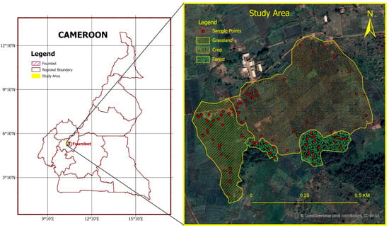
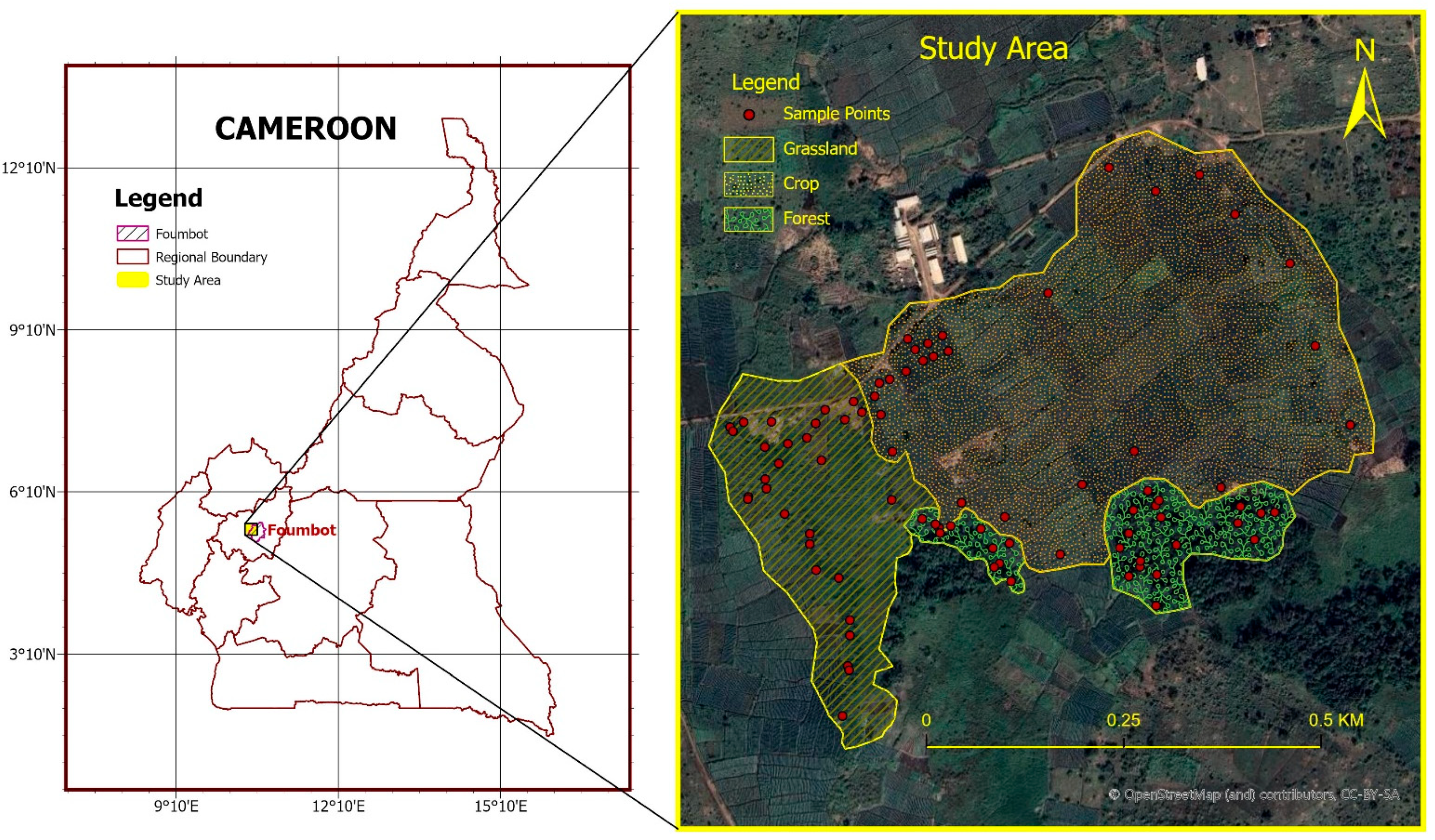
The study was conducted at the Institute de Recherche Agricole pour le Développement (IRAD) in Foumbot, western Cameroon, located at 1009 m altitude, between 5.4737° and 5.4772° N latitude and 10.5610° and 10.5628° E longitude (Figure 1). Foumbot has a tropical savanna climate (Aw) with a distinct rainy season from March to October and a dry season from November to February. Mean annual temperature is about 23 °C, while average annual rainfall ranges from 1595 to 1930 mm. The natural vegetation belongs to the forest–savanna transition zone, although much of the original vegetation has been converted into a mosaic of cropland, grassland, and remnant forest patches due to intensive agricultural activities [5]. The soils developed from volcanic parent materials, mainly volcanic ash, pyroclastic deposits, and basalt-derived materials associated with the Cameroon Volcanic Line. The dominant soils are Andisols in less-weathered positions and Oxisols in strongly weathered areas, corresponding to the occurrence of Andosols and Ferralsols reported for the Foumbot volcanic landscape [5].
Figure 1.
Geographic location of the study area in Foumbot (West Cameroon) and spatial distribution of sampling points across major land use types (grassland, cropland, and forest).
2.2. Sampling Method
The sampling design was stratified by land use category, with 30 soil sampling locations established in each of the three categories (cropland, grassland, and forest), yielding 90 sampling locations in total. Equal allocation was adopted to ensure balanced representation of the three land use categories for comparing soil properties and SOC stocks. Although a stratified random sampling approach was initially planned, some pre-selected locations had to be adjusted to accommodate field conditions and accessibility constraints, including flooded areas, standing crops, and irrigation infrastructure. Consequently, the final sampling locations were determined based on field accessibility and other practical considerations, while accounting for land use distribution and variations in soil and landscape conditions within each category. Efforts were also made to maintain a relatively uniform spatial distribution of sampling points across the study area.
At each sampling point, a circular plot with a radius of 2 m was delineated around the recorded coordinates. For each of the two depth intervals (0–10 and 10–20 cm), five soil subsamples were collected, one at the center of the plot and four along its circumference in perpendicular directions. The five subsamples from each depth interval were thoroughly mixed in equal volumes to form one composite sample per sampling point and depth. Samples from different sampling points and depth intervals were kept separate and were not pooled. Disturbed soil samples were collected for laboratory analysis of organic carbon (OC), while undisturbed soil cores at the same subsampling positions for bulk density determination. This resulted in a total of 180 composite soil samples for laboratory analysis (90 sampling points × 2 soil depths).
To characterize the pedological variability in the landscape, three representative soil profiles were opened along a toposequence corresponding to the upper slope, mid-slope, and lower slope positions. The profiles were morphologically described following standard soil survey procedures, including horizon designation, color, texture, structure, root abundance, pore distribution, and redoximorphic features. The resulting information was used to interpret the influence of soil-forming processes and landscape position on SOC distribution.
The geographical coordinates of all sampling locations were recorded for subsequent spatial analysis and geostatistical mapping of soil SOC stocks using Ordinary Kriging and Inverse Distance Weighting interpolation methods.
2.3. Laboratory Analysis
Bulk density was determined using the Blake undisturbed core method [13]. Undisturbed soil cores of 100 cm3 were collected using a ring cutter and oven-dried at 105 °C to constant mass. Bulk density was calculated from the oven-dry soil mass and the known core volume. Measurements from the cores collected at the same sampling point and depth interval were averaged to obtain one bulk density value for each point and depth.
Soil organic carbon (OC) content was determined in the composite soil samples using the acid dichromate wet oxidation method [14]. The resulting OC values were recorded for each sampling point and depth interval and subsequently used, together with the corresponding bulk density values, to calculate SOC stocks.
2.4. Data Analysis
2.4.1. Calculation of SOC Stocks
Soil organic carbon (SOC) stocks were calculated for each sampling point and depth interval using the organic carbon content, bulk density, and thickness of the sampled soil layer, consistent with the methodological approaches discussed by [15,16]. The calculation was performed using the following Equation (1):
where is the soil organic carbon stock (t C ha−1), (OC) is the organic carbon content (%), (BD) is the soil bulk density (g cm−3), and (d) is the soil-layer thickness (cm). With these units, the equation directly yields SOC stock in t C ha−1 without an additional conversion factor. Coarse fragment content was not incorporated into the calculation because no coarse fragments were observed in the sampled soil layers.
Each sampling location was assigned to its corresponding land use category (cropland, grassland, or forest). The calculated SOC stocks were grouped by land use category, and mean SOC stocks were calculated separately for each category and depth interval to facilitate comparisons among land uses.
2.4.2. Assessment of Data Distribution/Normality
Statistical analyses were performed using IBM SPSS Statistics version 26.0 to characterize the distribution of soil properties and evaluate differences among land use types and soil depths. Data normality was assessed using the Kolmogorov–Smirnov test at a significance level of p < 0.05. Variables that satisfied the assumption of normality, that is SOC stocks and pH-KCL, were analyzed using one-way analysis of variance (ANOVA). When significant differences were detected, Tukey’s honestly significant difference (HSD) test was applied for post hoc pairwise comparisons. Variables that did not satisfy the normality assumption, specifically bulk density (BD) and soil organic carbon (OC) concentration, were analyzed using the Kruskal–Wallis test to evaluate differences among groups. In addition, boxplots were used to visualize the distribution of and variability in soil properties across land use types and soil depths, thereby facilitating comparisons among all sampled combinations.
2.4.3. Spatial Modeling
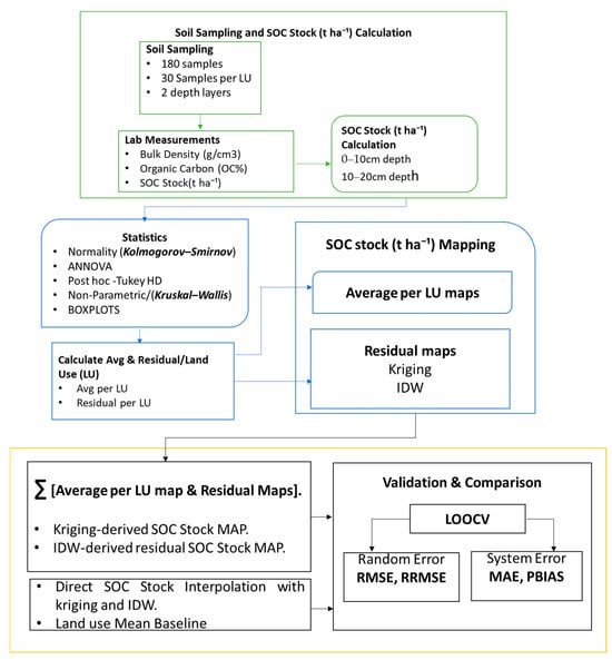
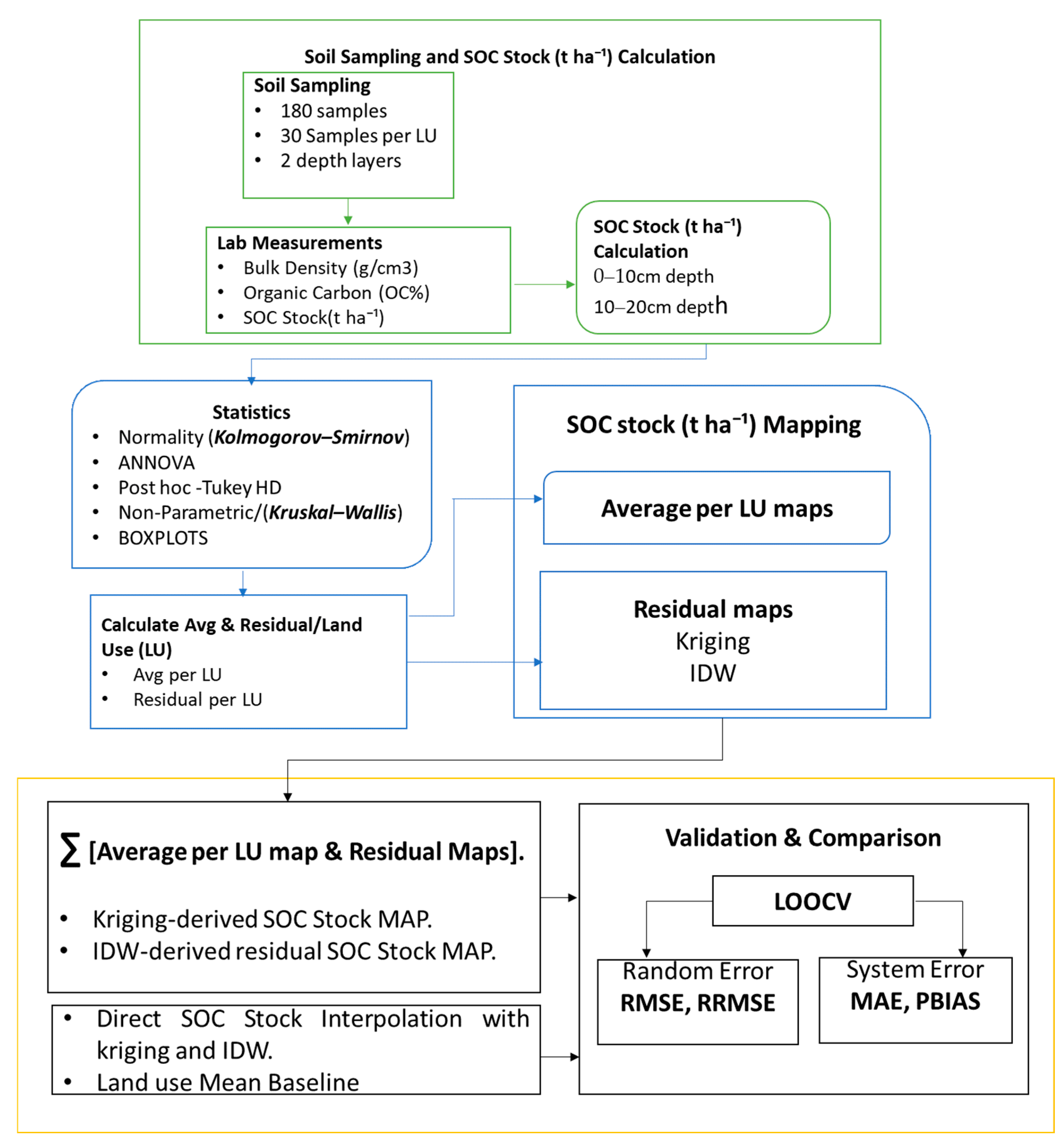
The spatial interpolation framework adopted in this study consisted of a two-step residual-based modeling approach (Figure 2). The objective was to remove systematic variability associated with land use units (LU) before modeling the remaining spatial dependence. Separating systematic land use effects from residual spatial variation before geostatistical interpolation is a well-established approach in spatial soil property modeling, as it can improve the representation of residual spatial dependence [17,18]. In the first step, the mean value of soil organic carbon (SOC) stock was calculated for every land use unit (LU) at each sampling depth to represent the characteristic baseline condition of that LU. The LU-specific mean was computed in Equation (2) as follows:
where is the mean value of soil organic carbon stock for a given land use unit (LU) at depth (d). is the observed value at sampling location (i), and (n) is the number of samples within the land use unit and depth.
Figure 2.
Workflow of soil sampling, SOC stock estimation, spatial mapping, and accuracy assessment. Green, blue, and orange represent the three main stages of the workflow: soil sampling and SOC stock (t ha−1) calculation, statistical analysis, and SOCS mapping, validation, and comparison, respectively. Arrows indicate the sequence and flow of activities from the initial soil sampling stage to the final validation and comparison stage.
In the second step, the residual value for each sampling location was calculated in Equation (3) as the difference between the observed value and the corresponding LU-specific mean:
where is the residual at sampling location (i), is the observed SOC value, and is the mean value of the corresponding land use unit (LU) at the same sampling depth.
The residuals represent the local spatial variation that remains after accounting for differences among land use units. They therefore capture the spatial variability within each land use unit, providing data that are more suitable for geostatistical modeling. The residual dataset was subsequently used as the input for spatial interpolation using Ordinary Kriging (OK) and Inverse Distance Weighting (IDW). By interpolating the residuals instead of the original observations, the method models the spatial autocorrelation that remains after accounting for differences among land use units. The final SOC prediction maps were then produced by adding the interpolated residuals to the corresponding mean SOC value for each land use unit:
2.5. Geostatistical Analysis
2.5.1. Semivariogram Analysis
Semivariogram analysis was used to characterize the spatial dependence of soil organic carbon (SOC) and to predict its distribution at unsampled locations across the different land use types. The semivariogram describes the change in semivariance as a function of separation distance and serves as the basis for evaluating spatial autocorrelation in soil properties [19]. The semivariogram was computed as Equation (4).
where γ(h) is the semivariance at lag distance h, and N(h) is the number of data pairs separated by distance h. Z(xi) and Z(xi + h) are SOC values at location xi and xi + h respectively.
Semivariograms were fitted with theoretical models to derive the key geostatistical parameters essential for spatial interpolation, specifically the nugget (C0), partial sill (C1), total sill (C0 + C1), and range (a). In this study, the Gaussian model was selected for semivariogram fitting because it provided a better representation of the observed spatial structure of SOC stock residuals. The Gaussian model is widely used to describe the spatial variability in soil properties and SOC stocks [20,21].
2.5.2. Ordinary Kriging (OK)
Ordinary Kriging focuses on the spatially correlated component and uses the fitted semivariograms directly for interpolation [22]. In this study, OK was applied to both the original SOC stock values (direct interpolation) and the residuals from the land use-based model (residual-based interpolation). For the residual-based approach, the interpolated residuals were added to the corresponding land use-specific mean SOC stocks to produce continuous SOC stock maps. The OK estimator is expressed as Equation (5):
where is the estimated SOC value at unsampled location X0, is the observed SOC value at the ith location, Wi is the kriging weight assigned to the ith observation and (s) is the total number of neighboring sample points used for prediction.
The Ordinary Kriging weights were determined from the fitted semivariogram model and set so that they sum to one, thereby ensuring unbiased predictions while minimizing the estimation variance, as described by [23,24]. Following semivariogram modeling, OK was applied to predict SOC residual values at unsampled locations and produce continuous spatial distribution maps. Unlike deterministic interpolation methods, OK incorporates the spatial autocorrelation structure quantified by the semivariogram [25], to generate optimal spatial predictions while minimizing the associated estimation variance. The degree of spatial dependence was assessed using the nugget-to-total-sill ratio, calculated as Equation (6)
where C0 is the nugget variance and C0 + C1 is the total sill. Following [26], spatial dependence was classified as strong when the nugget-to-total-sill ratio was <25%, moderate when it ranged from 25% to 75%, and weak when it was >75%.
2.5.3. Inverse Distance Weighting Interpolation (IDW)
Inverse Distance Weighting (IDW) was employed as a deterministic interpolation method to estimate soil organic carbon (SOC) values at unsampled locations. The method is based on the assumption that observations closer to the prediction location exert a greater influence on the estimated value than observations farther away. Consequently, the contribution of each neighboring sample decreases with increasing distance from the prediction point. The IDW estimator is expressed as Equation (7):
where Z0 is the estimated SOC value at point 0, Zi is the observed SOC value at known location i, di is the Euclidean distance between prediction location 0 and sample location i, (s) is the total number of known points used in estimation, and k is the specified power. Higher values of (k) assign greater influence to nearby observations and reduce the contribution of more distant samples, whereas lower values distribute the weights more uniformly among neighboring points [27]. IDW was implemented as a deterministic interpolation method for comparison with Ordinary Kriging. The predictive performance of both methods was subsequently evaluated using interpolation accuracy statistics to identify the method that best represented the spatial distribution of SOC across the study area.
2.5.4. Mean per Land Use Baseline
A mean per land use baseline was established to provide a reference against which the predictive performance of direct and residual-based interpolation methods could be evaluated. Baseline predictions were generated using LOOCV, a commonly used approach for assessing predictive performance by excluding individual observations in turn and comparing predicted and observed values [28]. For each heldout observation, the mean SOC stock of its corresponding land use class was recalculated using the remaining observations in that class. The predicted SOC stock was then calculated as Equation (8):
where is the predicted SOC stock for the held-out observation (i). is the observed SOC stock at location (j) and is the number of observations in the land use class containing observation (i). The condition ensures that the held-out observation is excluded from calculating its prediction. The resulting predictions were evaluated using RMSE, MAE, RRMSE and PBIAS. The baseline provides a simple benchmark based on land use-related differences in mean SOC stocks, allowing the additional predictive value of spatial interpolation to be assessed [29].
2.6. Cross-Validation
The predictive performance of the interpolation models was evaluated using LOOCV in the Geostatistical Analyst extension of ArcGIS 10.5. Accuracy was assessed using root mean square error (RMSE; Equation (9)), relative root mean square error (RRMSE; Equation (10)), mean absolute error (MAE; Equation (11)), and percent bias (PBIAS; Equation (12)). RMSE, RRMSE and MAE quantified prediction errors, whereas PBIAS assessed systematic over- or underestimation; lower error values and PBIAS values closer to zero indicated better performance. The use of cross-validation and multiple accuracy metrics is consistent with SOC mapping studies in Cameroon and other African regions [10,30], while global studies have similarly shown that interpolation performance varies according to spatial structure, sampling density and soil depth [19]. Therefore, IDW and OK were compared empirically to identify the method that most reliably predicted SOC across the Foumbot Plains.
where 1 n is the number of measured samples, SOCobs(i) the observed concentration of the SOC measurement (t C ha−1), and SOCpred(i) the predicted concentration of the SOC measurement (t C ha−1).
3. Results
3.1. Morphological Characterization of Soil Profiles
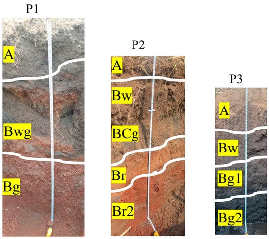
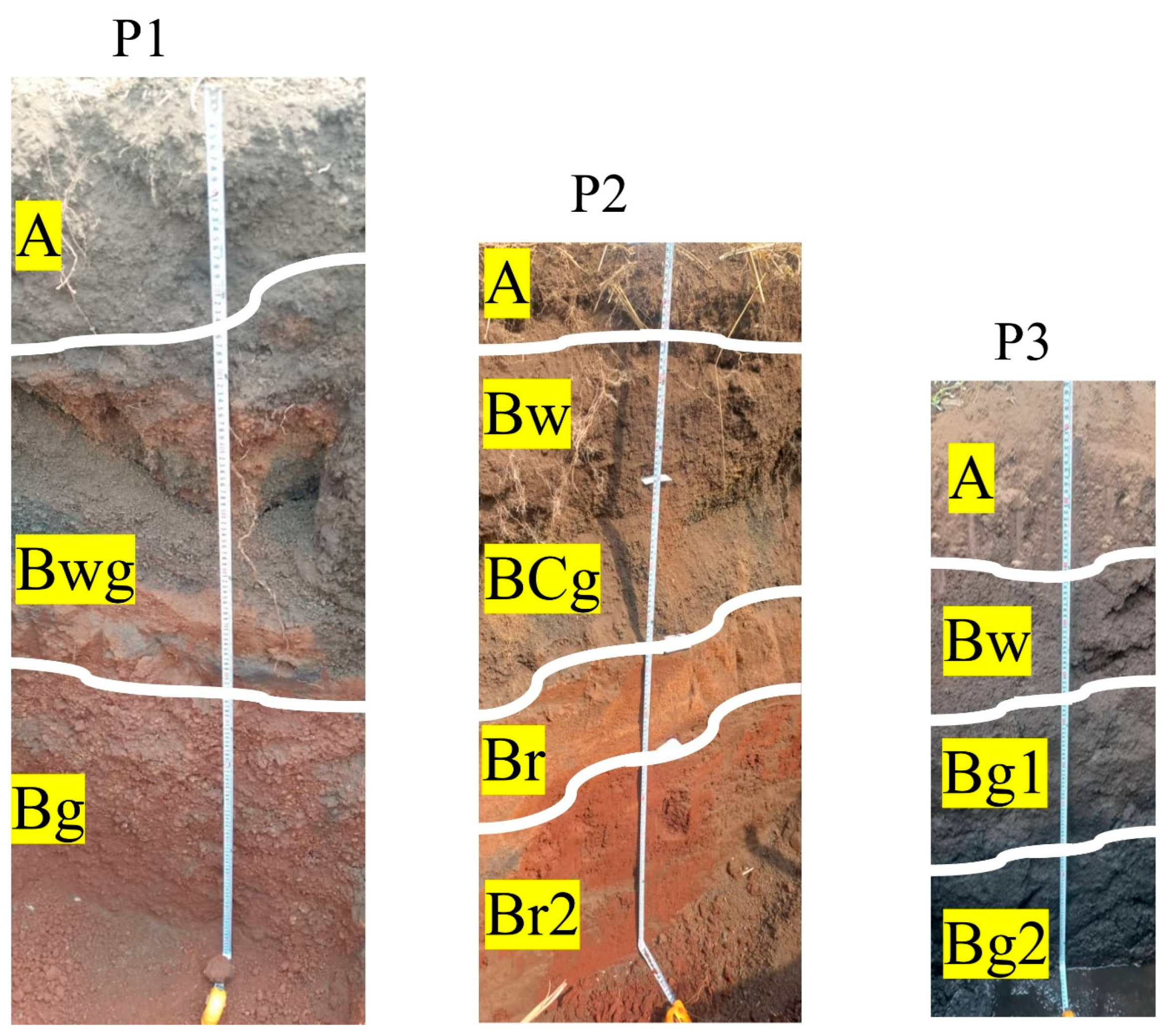
The three representative soil profiles exhibited marked morphological differences along the toposequence, indicating variations in pedogenic processes and drainage conditions. Figure 3 shows a progressive transition from well-drained upland soils toward hydromorphic soils in lower landscape positions.
Figure 3.
Morphological characterization of the three representative soil profiles showing horizon boundaries and field horizon designation.
Profile P1, located at the upper slope position, consisted of three horizons: A (0–35 cm), Bwg (35–85 cm), and Bg (>85 cm). The surface horizon displayed a dark grayish-brown color (10YR 4/2), clay texture, and moderate fine-to-medium subangular blocky structure. The subsurface horizons were characterized by reddish mottles and pronounced redoximorphic features, indicating periodic water saturation and iron redistribution. The Bg horizon showed strong redox concentrations and depletions associated with a coarse angular blocky structure.
Profile P2, situated at the mid-slope position, exhibited five horizons: A (0–20 cm), Bw (20–45 cm), BCg (45–70 cm), Br (70–95 cm), and Br2 (>95 cm). The profile was characterized by a transition from a dark brown surface horizon to strongly developed red subsoil horizons. The lower horizons displayed strong red colors (2.5YR 4/6), clay texture, and moderate-to-strong angular blocky structures, suggesting advanced weathering and iron accumulation. Redox features were mainly observed in the BCg horizon.
Profile P3, located at the bottom slope position, consisted of four horizons: A (0–25 cm), Bw (25–50 cm), Bg1 (50–80 cm), and Bg2 (>80 cm). The profile exhibited darker colors and increasingly hydromorphic conditions with depth. The Bg2 horizon was very dark gray to black, displayed weak blocky to massive structure, and showed strong gleying features indicative of prolonged saturation.
3.2. Statistical Analysis of Soil Properties
3.2.1. Land Use and Depth-Dependent Variations in Soil Physiochemical Properties
One-way ANOVA revealed significant differences in SOC stocks and pH-KCl among land use categories at both soil depths (p < 0.001; Appendix A, Table A1). The magnitude of these differences varied with depth. For pH-KCl, the F-value was higher at 10–20 cm (F = 64.036) than at 0–10 cm (F = 42.232), whereas SOC stock showed the opposite pattern, with a higher F-value at 0–10 cm (F = 41.233) than at 10–20 cm (F = 15.184).
Tukey’s HSD post hoc test identified the specific land use pairs responsible for these differences (Appendix A, Table A2). For SOC stocks, grassland and forest did not differ significantly at 0–10 cm (p = 0.232), but their difference was significant at 10–20 cm (p = 0.041). The mean differences between grassland and cropland, and between cropland and forest, decreased with depth, from 31.17 to 14.70 and from 38.60 to 26.69, respectively. In contrast, pH-KCl differed significantly among all land use pairs at both depths (all p < 0.001). The mean differences between grassland and cropland and between grassland and forest increased with depth, from 1.043 to 1.303 and from 0.580 to 0.864, respectively, whereas the difference between cropland and forest decreased slightly, from 0.463 to 0.439.
For organic carbon (OC) and bulk density (BD), Kruskal–Wallis post hoc comparisons revealed further differences among land use types (Appendix A, Table A3). At both depths, OC differed significantly between cropland and each of the other two land uses (all adjusted p < 0.001), whereas the difference between grassland and forest was not significant (adjusted p = 0.209 at 0–10 cm and 0.301 at 10–20 cm). BD differed significantly among all land use pairs at 0–10 cm (all adjusted p < 0.001). At 10–20 cm, all land use pairs also differed significantly, although the difference between grassland and forest was smaller (adjusted p = 0.011). Thus, while OC did not differ significantly between grassland and forest at either depth, BD differed significantly between these two land uses at both depths.
3.2.2. Boxplot Visualization of Land Effect on SOC-Related Soil Properties
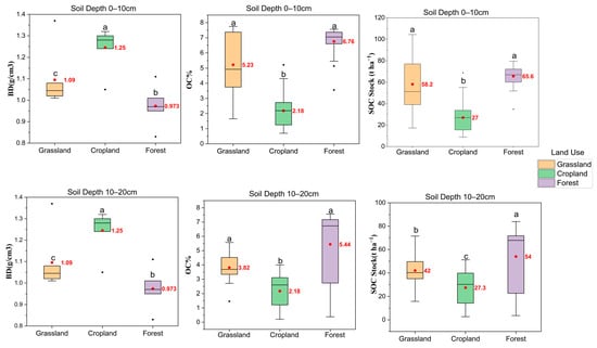
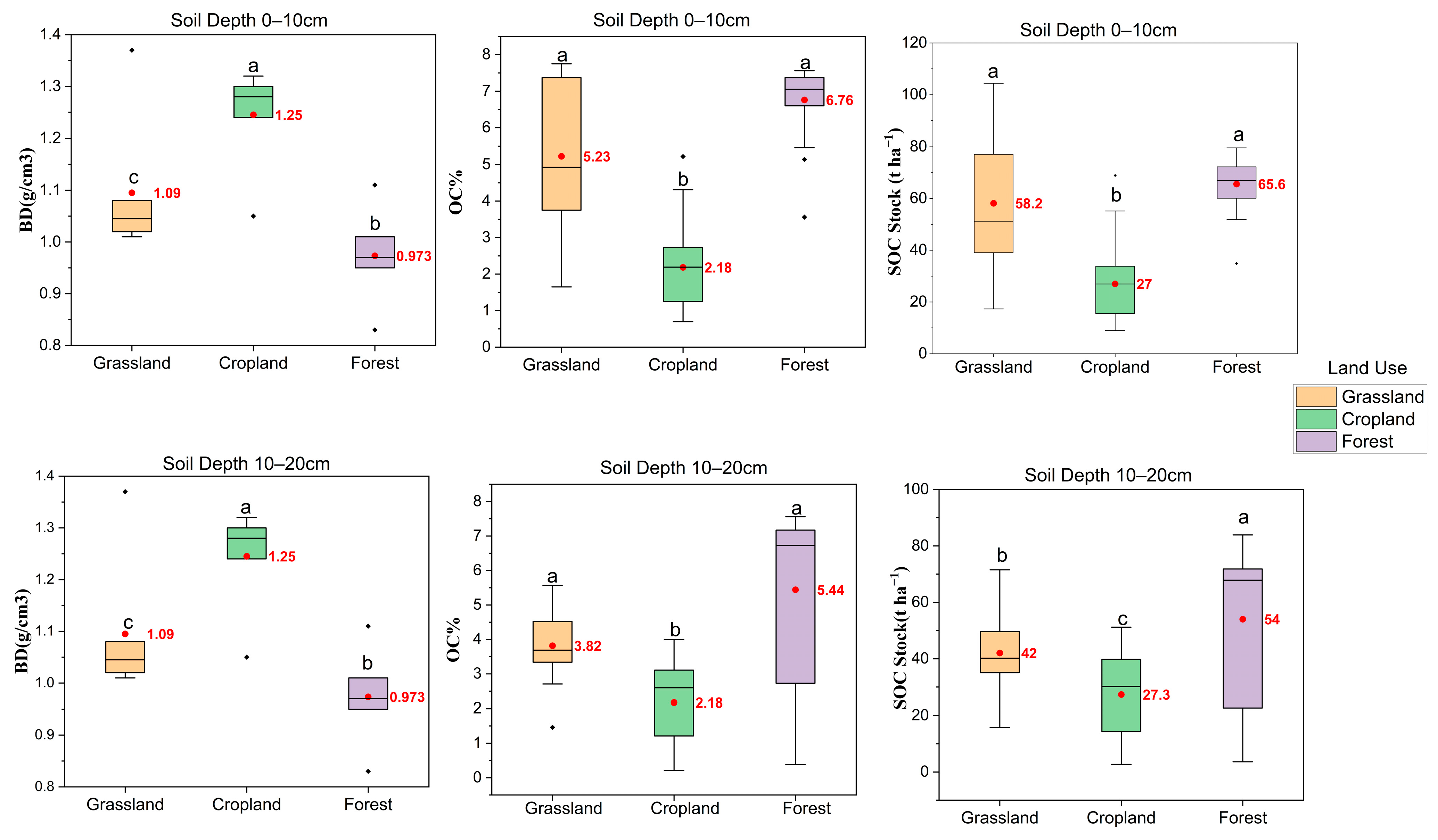
Figure 4 presents the distributions of BD, OC, and SOC stocks (SOCSs) across the three land use types at 0–10 cm and 10–20 cm soil depths. The boxplots reveal contrasting patterns in soil physical and carbon-related properties. BD was highest in cropland (1.25 g cm−3), followed by grassland (1.09 g cm−3) and forest (0.97 g cm−3), with identical values recorded at both soil depths (0–10 and 10–20 cm). In contrast, OC levels were highest in forest (6.76% at 0–10 cm and 5.44% at 10–20 cm) and grassland (5.23% and 3.82%, respectively), while cropland had the lowest values (2.18% at both depths). SOCS followed a similar pattern, with higher values in forest (65.6 and 54.0 t ha−1) and grassland (58.2 and 42.0 t C ha−1), than in cropland (27.0 and 27.3 t C ha−1), at 0–10 cm and 10–20 cm, respectively. While SOCS declined with depth in forest and grassland, it remained nearly unchanged in cropland. Overall, the distributions highlight contrasting soil conditions across land use types, with forest and grassland showing higher OC levels and SOCS, whereas cropland exhibited higher BD.
Figure 4.
Distribution of bulk density (BD), organic carbon (OC), and SOCS across land use types and soil depths. Boxes represent the interquartile range, horizontal lines within the boxes represent medians, and whiskers extend to 1.5 times the interquartile range. Black dots represent outliers, while red dots and adjacent values indicate means. Different lowercase letters indicate significant differences among land uses at the same soil depth (p < 0.05).
3.3. Spatial Dependence of SOCS
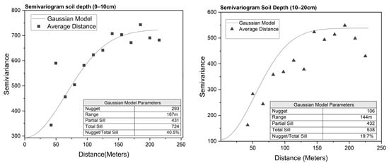
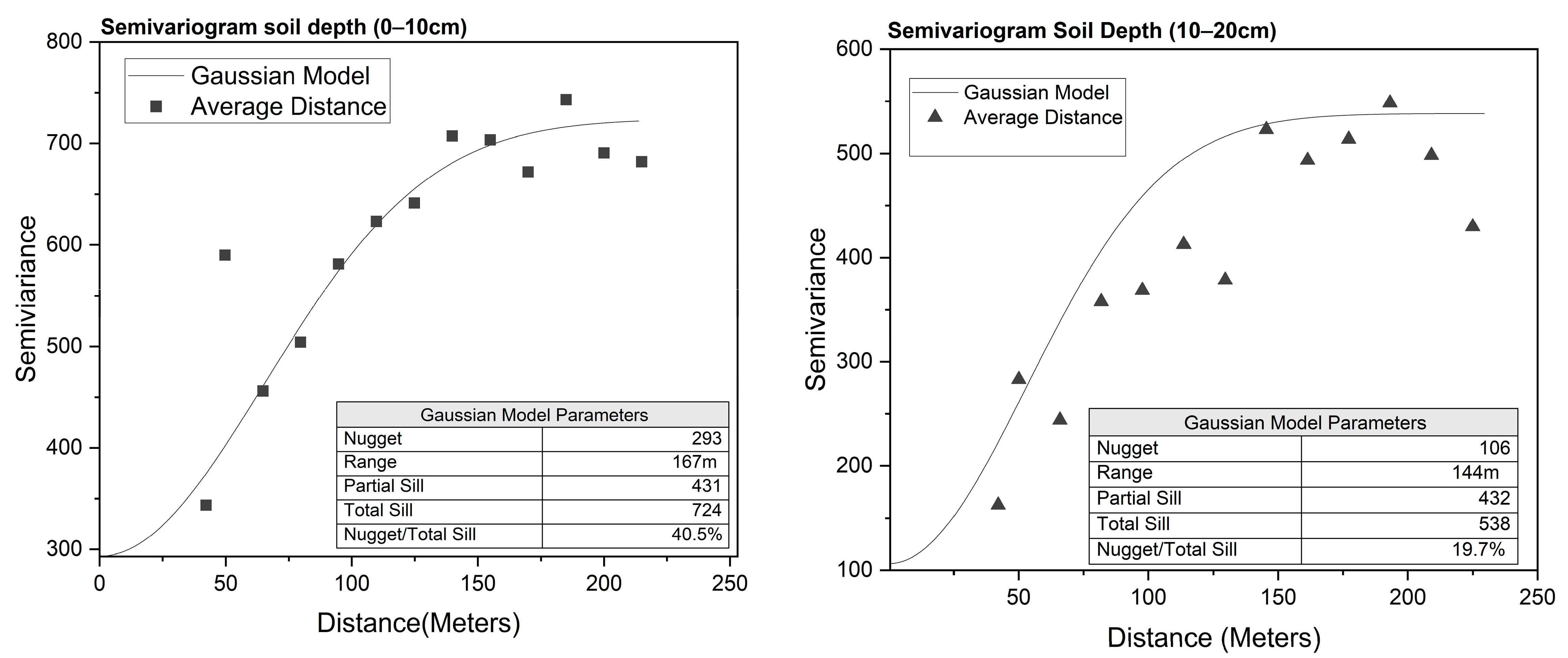
As shown in Figure 5, the fitted Gaussian semivariogram models revealed spatial dependence in the residual component of SOCS at both soil depths, indicating that the residuals exhibited spatial structure after accounting for differences among land use classes, with spatial ranges of approximately 167 m and 144 m for the 0–10 cm and 10–20 cm layers, respectively. At 0–10 cm, the nugget was 293, partial sill 431 and total sill 724, giving a nugget-to-total-sill ratio of 40.5%, indicating moderate spatial dependence, following the method of [26]. In contrast, the 10–20 cm layer had a substantially lower nugget (106) and a similar partial sill (432) and total sill 538, resulting in a nugget-to-total-sill ratio of 19.7%, indicating strong spatial dependence. Although the surface layer exhibited a slightly longer spatial range, its higher nugget indicates greater microscale variability, potentially associated with localized factors such as vegetation cover, litter accumulation, farming practices and land use management. Conversely, the lower nugget and stronger spatial dependence at 10–20 cm suggests greater spatial continuity, potentially reflecting the combined influence of relatively continuous ecological processes, including root penetration, vertical carbon transfer, soil formation, and organic matter redistribution, together with reduced exposure to localized surface disturbances.
Figure 5.
Spatial dependence of soil organic carbon stock across soil depths.
3.4. Performance of Interpolation Methods
The performance of the interpolation methods was evaluated using LOOCV. At 0–10 cm, residual IDW achieved the lowest RMSE (15.69 t C ha−1) and MAE (9.81 t C ha−1), with an RRMSE of 31.24% and a PBIAS of −0.33% (Table 1). Residual OK produced similar results, with an RMSE of 15.82 t ha−1, MAE of 10.50 t ha−1, RRMSE of 31.49% and PBIAS of 0.59%. Both residual-based methods performed better in terms of RMSE and MAE than direct IDW and OK, which had RMSE values of 19.60 and 18.73 t C ha−1, respectively, and the land use mean baseline (17.76 t C ha−1). At 10–20 cm, residual OK achieved the lowest RMSE (14.28 t C ha−1) and RRMSE (34.74%), whereas residual IDW had the lowest MAE (10.11 t C ha−1). Their respective PBIAS values were −0.57% and −6.36%. Direct OK and IDW had RMSE values of 16.27 and 17.30 t C ha−1 respectively, while the land use mean baseline had an RMSE of 19.11 t C ha−1. Overall, residual-based interpolation yielded the lowest RMSE at both depths, although the best-performing method varied with depth and evaluation metric.
Table 1.
Cross-validation performance of the mean per land use baseline, direct interpolation, and residual-based interpolation methods for soil organic carbon stocks at 0–10 and 10–20 cm soil depths. Bold values indicate the best performance for each statistical measure at each soil depth, based on the lowest RMSE, MAE and RRMSE, and the PBIAS value closest to zero.
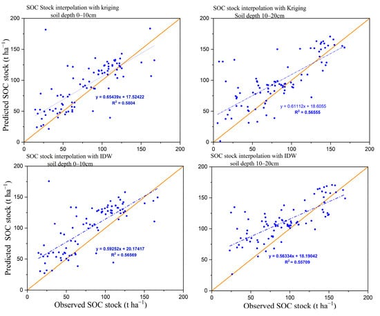
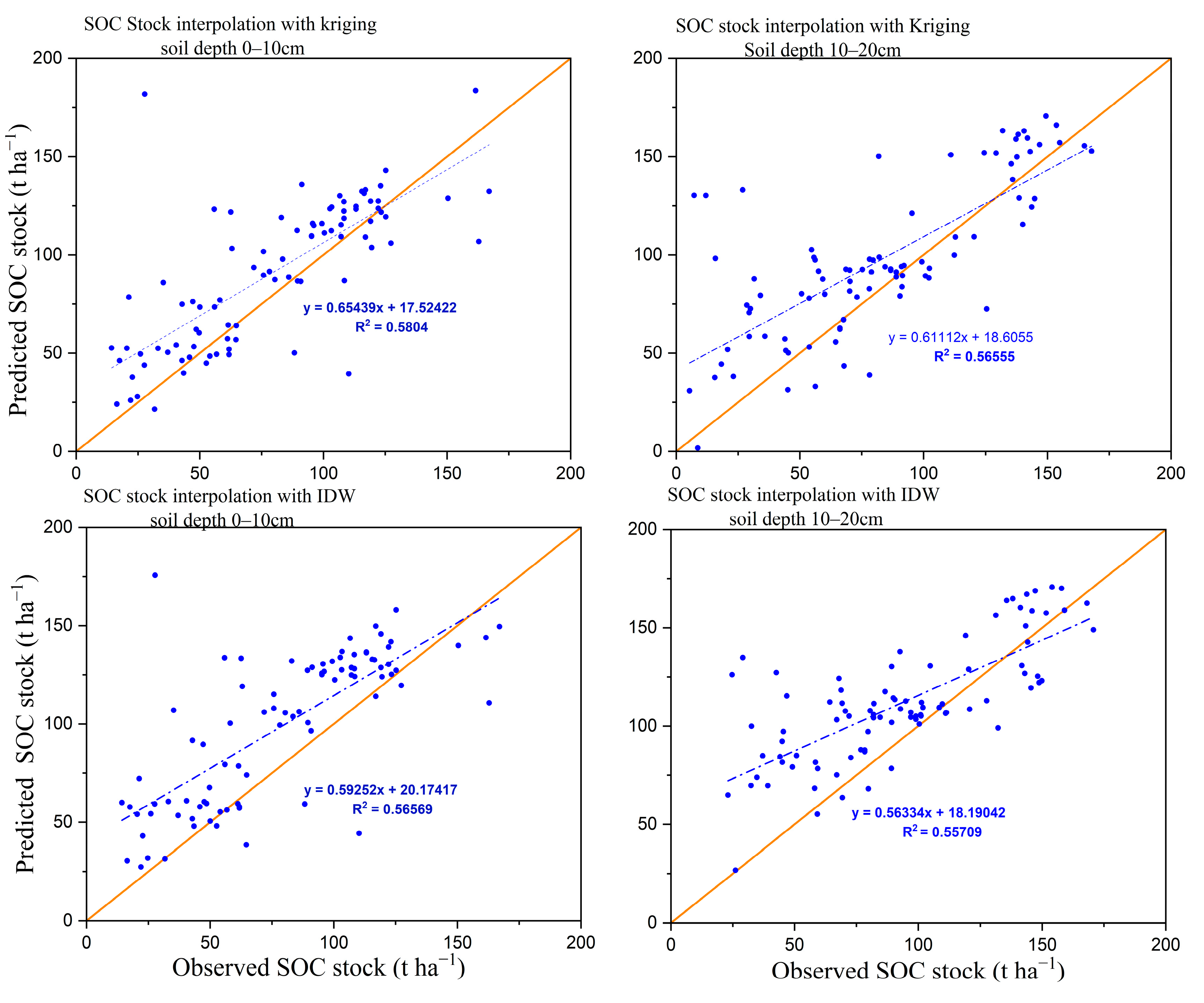
Scatterplots of observed versus predicted SOCS (Figure 6) further confirmed the ability of the residual-based interpolation approach to capture the general variation in SOCS. However, a tendency toward systematic over- and underprediction was observed. The regression slopes ranged from 0.563 to 0.654 and were consistently below one, indicating that the interpolation models tended to underestimate higher SOCS and overestimate lower SOCS. This tendency was particularly evident at the 10–20 cm depth, while the underprediction of higher SOCS was more pronounced for OK at 0–10 cm. Overall, this pattern suggests that the residual-based spatial modeling approach appeared to smooth extreme SOCS values during spatial prediction. Such smoothing is consistent with the known difficulty of spatial interpolation methods in reproducing extreme observations, which are more difficult to reproduce from surrounding observation [31].
Figure 6.
Observed versus predicted SOC stock from OK and IDW interpolation across soil depths. Blue dots represent LOOCV samples, the blue dashed line represents the fitted linear regression between observed and predicted SOC stocks, and the solid orange line represents the1:1 line (perfect agreement between observed and predicted values.
3.5. Comparison of Ordinary Kriging and IDW Maps
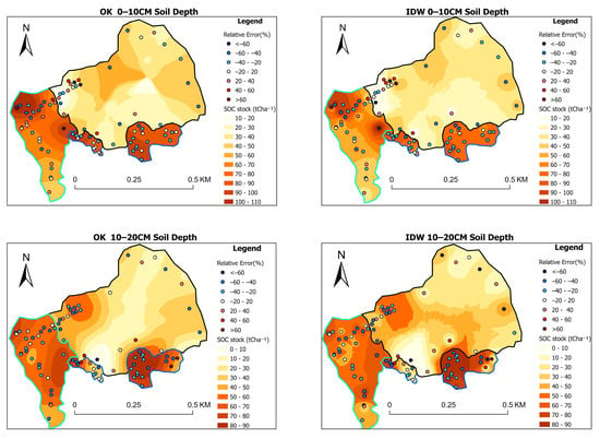
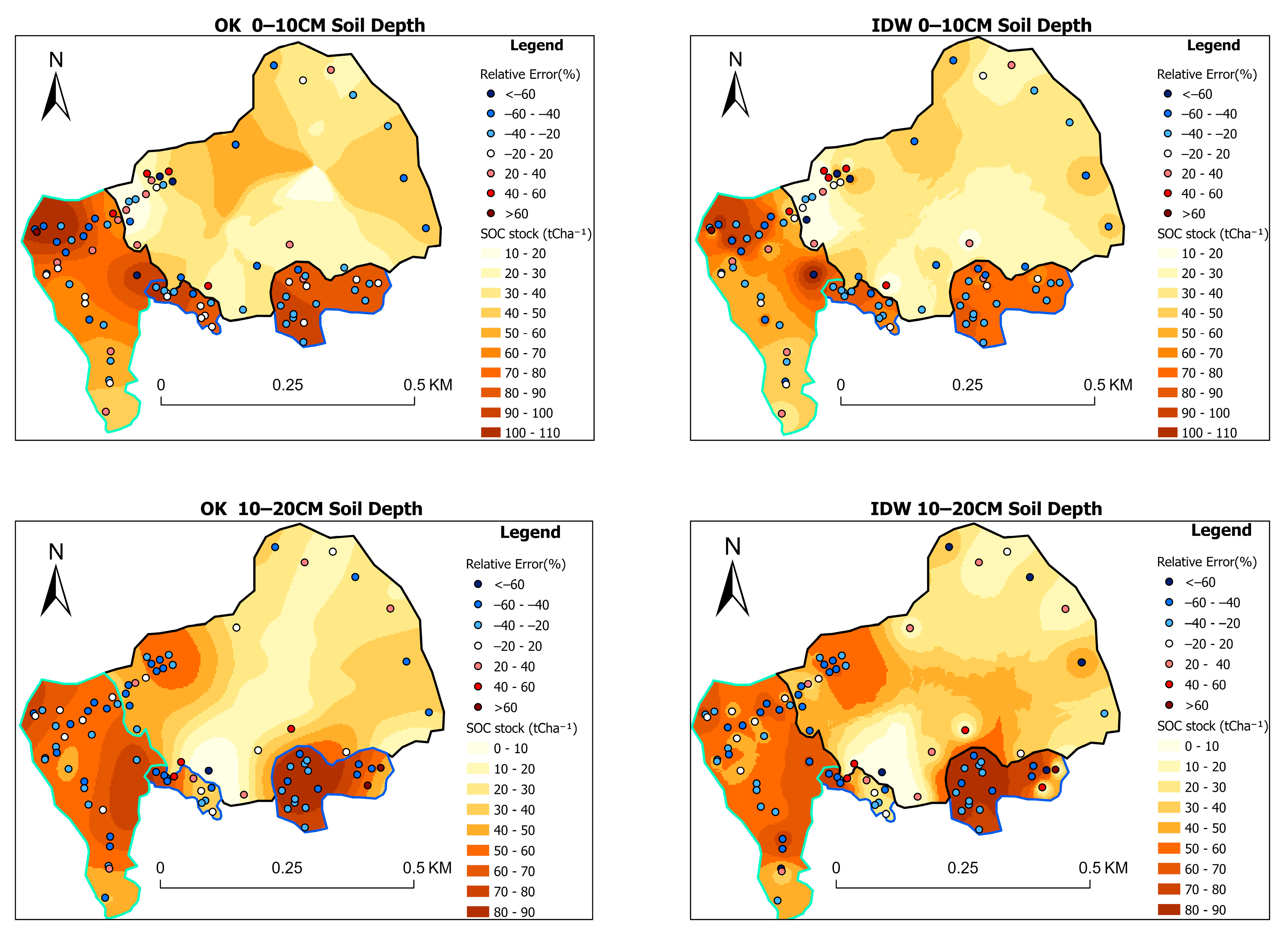
Visual comparison of the interpolated maps (Figure 7) indicated that both methods reproduced similar broad-scale spatial patterns of SOCS. However, OK generated smoother spatial transitions and more continuous prediction surfaces, while IDW produced more localized variations around sampling locations. These differences were particularly evident in the 10–20 cm and 0–20 cm layers. At 0–10 cm, SOCSs were generally higher in the southwestern and southeastern parts of the study area, corresponding mainly to grassland and forest areas, with values approximately ranging from 50 to 90 t C ha−1. Lower values (approximately 10–40 t C ha−1) were mainly distributed across the central and northern areas, which are largely under cropland. Although cropland occupies a substantial proportion of the study area, the sampling design allocated equal numbers of samples to each land use category to facilitate comparisons among land uses. Therefore, the mapped patterns should be interpreted in light of the spatial distribution of the sampling points, particularly across the extensive cropland areas. At 10–20 cm, SOCSs were generally lower than in the surface layer, although relatively high SOCSs remained concentrated in the western and southeastern zones, mainly in grassland and forest areas, with localized values exceeding 60 t C ha−1.
Figure 7.
Final SOC stock (t ha−1) maps generated using Ordinary Kriging (OK) and Inverse Distance Weighting (IDW) interpolation for two soil depth intervals. Green, blue, and black polygon outlines represent grassland, forest, and cropland areas, respectively.
Overall, the results indicate substantial spatial heterogeneity in SOCS across the study area, and both OK and IDW reproduced the broad spatial distribution patterns. Comparison with the mean per land use baseline and direct interpolation showed that residual-based interpolation generally provided more accurate predictions at both depths. However, neither IDW nor OK consistently outperformed the other across all evaluation metrics. At 0–10 cm, residual IDW performed slightly better than residual OK, with lower RMSE, MAE and RRMSE, whereas at 10–20 cm, residual OK had a marginally lower RMSE and RRMSE, while residual IDW retained a lower MAE. Thus, the relative performance of the two methods varied with soil depth and the evaluation metric.
4. Discussion
4.1. Soil Organic Carbon Stock Variability in Relation to Land Use and Soil–Landscape Conditions in the Foumbot Agricultural Basin
Soil organic carbon stocks (SOCSs) varied substantially across the Foumbot agricultural landscape, with significant differences among land use categories at both sampled depths. Across the upper 20 cm, SOCS was highest under forest (119.6 t C ha−1), followed by grassland (100.2 t C ha−1) and cropland (54.3 t C ha−1). SOCS differed significantly among land use categories at both depths (p < 0.001), with more pronounced differences in the surface layer (F = 41.233) than in the subsurface layer (F = 15.184). These results indicate a clear association between land use and SOCS in Foumbot.
The higher SOCS under forest and grassland is consistent with findings from the Noun Plain and the forest–savanna transition zone of Cameroon, where greater SOCSs have been reported under natural vegetation than under cultivated land [3,4]. Similar land use-related differences have also been reported in Mount Cameroon [2], and other parts of West and Central Africa [32,33]. Such patterns may reflect differences in organic matter inputs, root biomass, vegetation cover, and management practices. In cropland, crop residue removal and repeated soil disturbance may reduce organic matter inputs or alter soil conditions favorable to carbon retention. Such mechanisms provide plausible explanations for the observed SOCS differences.
The depth-specific results further illustrate how SOCS is distributed across the studied land uses. At 0–10 cm, mean SOCS was 65.6 t C ha−1 under forest, 58.2 t C ha−1 under grassland and 27.0 t C ha−1 under cropland. At 10–20 cm, the corresponding values were 54.0, 42.0 and 27.3 t C ha−1, respectively. The greater SOCS under forest and grassland in the surface layer may partly reflect the accumulation of litter- and root-derived organic inputs near the soil surface. However, significant differences among land uses were also observed at 10–20 cm, showing that the contrast in SOCS extended beyond the surface layer. SOCS also decreased with depth under forest and grassland, whereas the mean SOCS values remained nearly unchanged between the two depth layers under cropland.
Soil morphology provides additional context for understanding this spatial variation. Profile P1 exhibited redoximorphic features in the upper landscape position, P2 was characterized by strongly weathered red soils at the mid-slope position, and P3 showed hydromorphic characteristics in the lower landscape position. These morphological contrasts indicate variation in soil development and drainage conditions across the study landscape, which may influence SOC retention. For example, recurrent soil saturation can restrict decomposition under certain conditions and favor SOC preservation, while mineralogical properties associated with strongly weathered soils may influence organic matter stabilization. This interpretation is consistent with previous research documenting variations in soil morphology, mineralogy and classification along a climotoposequence in Foumbot [5]. Studies in other tropical landscapes have similarly associated SOC variability with topographic position, soil properties and vegetation characteristics [34,35]. In addition, interactions between organic matter and mineral phases can contribute to SOC stabilization in tropical soils [36,37]. However, mineral-associated organic carbon, reactive iron phases and decomposition rates were not directly measured in this study; therefore, their potential contributions should be regarded as possible mechanisms rather than established explanations for the observed SOCS patterns. Overall, the observed SOCS patterns may reflect the combined influence of land use and underlying soil landscape conditions.
Differences in bulk density (BD) and organic carbon (OC) concentration provide further insight into the observed SOCS patterns. BD was highest under cropland (1.25 g cm−3), followed by grassland (1.09 g cm−3) and forest (0.97 g cm−3), whereas OC levels followed the opposite pattern. At 0–10 cm, OC was highest under forest (6.76%), followed by grassland (5.23%) and cropland (2.18%), with a similar pattern observed at the 10–20 cm depth. The contrasting patterns of OC and BD highlight variations in soil properties across the study area, with cropland having lower OC levels and higher BD than forest and grassland. Although higher BD may be associated with soil compaction in cultivated areas, it can also reflect natural variation in soil properties across the landscape. Similar patterns of higher BD and lower SOCS under cultivated land have also been reported in northwestern Cameroon [38].
The observed SOCS differences have important implications for maintaining soil quality in the Foumbot agricultural landscape. The comparatively lower SOCS under cropland, together with lower OC levels and higher BD, points to less favorable soil conditions for maintaining organic carbon reserves than those observed under forest and grassland. Although the study did not directly quantify all the effects of SOCS on nutrient retention, aggregate stability, or water-holding capacity, maintaining organic matter inputs remains a relevant management consideration. Practices such as crop residue retention, cover cropping, agroforestry, reduced tillage and improved fallow management may help sustain SOCS, although their effectiveness will depend on local soil conditions and management constraints. Overall, the findings demonstrate clear differences in soil carbon status across land uses, with forest and grassland retaining greater SOCS than cropland across the upper 20 cm of soil. These findings underscore the need for land use-specific soil management strategies that promote organic matter retention and support climate-smart agricultural practices in the Foumbot landscape.
4.2. Spatial Dependence and Distribution of SOC Stocks
The semivariogram analysis revealed a clear depth-dependent pattern in the spatial organization of SOC across the Foumbot Plains (Figure 5). At 0–10 cm, SOCS showed moderate spatial dependence, with a nugget-to-sill ratio of 40.5%, indicating that its spatial pattern reflected both spatially structured variation and local-scale variability. Such variation may be associated with differences in vegetation cover, land use and farming practices. For example, cultivation intensity, manure application, organic inputs and distance from homesteads can contribute to spatial differences in SOCS within agricultural fields. Similar patterns have been reported in northern Ghana, where SOCS varied according to farming practices and organic inputs [39]. Research in southeastern Nigeria has also found substantial spatial variation in SOCS and highlighted the role of terrain characteristics [20].
In contrast, the 10–20 cm layer showed stronger spatial dependence, with a nugget-to-sill ratio of 19.7%. This indicates that SOCS at this depth followed a more consistent spatial pattern than those in the surface layer. One possible explanation is that deeper SOCSs are less directly affected by recent farming activities and surface disturbances. Instead, their distribution may be more closely related to soil properties and landscape conditions, such as topography, soil texture, parent material and drainage. A national assessment based on more than 1400 georeferenced soil profiles across Cameroon also found that SOCS varied with soil depth and environmental conditions [10]. Similarly, a study in Ghana identified climatic and soil-related factors, including soil erodibility, sand content and electrical conductivity, as important factors explaining SOCS distribution [40].
The estimated spatial ranges were 167 m at 0–10 cm and 144 m at 10–20 cm, indicating the approximate distances over which SOCS residuals at nearby locations remained spatially correlated. This information can help guide sampling design in future studies. Research in Miombo woodlands has shown that surface SOCS may vary with distance from trees, while deeper SOCS may be more closely related to clay content and topographic processes [41]. Although these factors were not tested individually in the present study, they may help explain the differences in spatial patterns between the two depths. The slightly shorter range at 10–20 cm suggests that spatial autocorrelation in the deeper layer operates over a somewhat shorter distance than in the surface layer. Therefore, sampling intervals should be considered in relation to the estimated spatial range, as well as the purpose of the study and the level of spatial detail required [8].
The observed spatial structure corroborates with previous research showing that SOCS distribution is associated with landscape and soil characteristics. Studies in tropical montane ecosystems have linked SOCS to topography, vegetation, land use and soil properties [36,37]. Other studies have shown that geostatistical methods can describe SOC variation and that factors such as elevation, vegetation indices and soil wetness can improve spatial prediction [6,42]. In the Foumbot Plains, the differences in SOCS among land use categories, together with the spatial dependence identified by semivariogram analysis, indicate that SOCS distribution varies across the landscape.
The final SOCS maps (Figure 7) showed broadly similar spatial patterns for Ordinary Kriging (OK) and Inverse Distance Weighting (IDW), although the predicted values differed in some local areas. Relatively high SOCS values were mainly observed in the western and southeastern parts of the study area, where grassland and forest were more common. Lower SOCS values were generally found in central and northern areas dominated by cropland. These mapped patterns are consistent with the differences observed among land use categories and provide a spatial representation of SOCS distribution across the Foumbot agricultural landscape.
The interpretation of the mapped SOCS patterns should also consider how the sampling points were distributed across the study area and the practical constraints encountered during fieldwork. Although the sampling locations were distributed at varying distances to support the analysis of spatial autocorrelation using semivariograms, this distribution may not have captured all local variations in SOCS equally well. Field accessibility constraints, like standing crops and irrigation infrastructure, necessitated adjustments to some sampling locations and may have limited the representation of certain local environmental conditions. Furthermore, the equal allocation of sampling points among land use categories was intended to facilitate comparisons of SOCS among land uses rather than to reflect their proportional coverage across the study area. Consequently, while the resulting maps provide a useful representation of the observed SOCS patterns, their spatial detail, particularly across the extensive cropland area, should be interpreted with these limitations in mind.
The comparison of interpolation methods showed that residual-based interpolation generally produced lower prediction errors than direct interpolation and the land use mean baseline. At 0–10 cm, residual IDW achieved the lowest RMSE (15.69 t ha−1), compared with 17.76 t ha−1 for the baseline, 19.60 t ha−1 for direct IDW and 18.73 t ha−1 for direct OK. At 10–20 cm, residual OK achieved the lowest RMSE (14.28 t ha−1), compared with 19.11 t ha−1 for the baseline, 17.30 t ha−1 for direct IDW and 16.27 t ha−1 for direct OK. These results suggest that accounting for differences among land use classes before interpolating the remaining variation can improve the prediction of SOCS. However, the relative performance of residual IDW and OK differed between depths and evaluation measures, meaning that neither method was consistently best under all conditions.
These findings agree with previous studies that used residual-based or combined modeling approaches to map SOC [9,11,43]. In Cameroon, Ref. [10] reported a modest improvement in SOCS prediction when residual interpolation was combined with machine learning models. Their study also found broadly similar performance between IDW and OK. Other studies have demonstrated the usefulness of direct geostatistical interpolation for mapping SOC [8,12,20,44]. For example, a study in Zambia reported an RRMSE equivalent to 58.18% of the mean observed SOC when using direct OK [12], compared with RRMSE values of 34.7–39.0% reported for the residual-based methods in the present study. Although differences in sampling design, soil depth, measured variables and validation methods make direct comparisons between studies difficult, the results support the usefulness of accounting for land use-related variation when predicting SOCS. In particular, the lower RMSE values obtained through residual-based interpolation indicate an improvement over direct interpolation and the land use mean baseline in this study.
The spatial distribution of SOCS provides a basis for identifying areas where soil carbon management could be prioritized in the upper 20 cm of the Foumbot agricultural basin. Areas with relatively low SOCS, particularly those dominated by cropland, may benefit from practices such as crop residue retention, cover cropping, organic amendments, conservation agriculture and agroforestry, depending on local soil and farming conditions. In areas with relatively high SOCS, maintaining vegetation cover and limiting unnecessary soil disturbance may help sustain existing carbon stocks. Local water conditions should also be considered in parts of the Foumbot Plains where groundwater tables are high. The maps therefore provide a spatial baseline that can support management prioritization and guide future SOCS monitoring.
Overall, this study contributes to SOC research in western Cameroon by examining both differences in SOCS among land use categories and their spatial distribution across the landscape. By combining soil profile observations, SOCS assessment, semivariogram analysis and spatial prediction, it provides an integrated approach for understanding and mapping SOCS in tropical volcanic agricultural landscapes.
5. Conclusions
This study assessed SOCSs and their spatial variability under the main land use systems of the Foumbot agricultural basin, western Cameroon. The findings showed that SOCSs varied across the landscape and were associated with land use, topography, and soil properties. These results highlight the importance of considering both land use differences and the wider soil and landscape conditions when assessing SOCSs.
The study also showed that SOCSs exhibited spatial dependence and could be mapped using geostatistical methods. Comparisons with direct interpolation and the land use mean baseline indicated that residual-based interpolation generally reduced prediction errors at both soil depths. Residual IDW performed best at 0–10 cm, while residual OK achieved the lowest RMSE at 10–20 cm. These findings suggest that accounting for land use-related differences before interpolating the remaining spatial variation can improve SOCS predictions, although the preferred interpolation method depends on soil depth and the evaluation metric.
The resulting maps provide a spatial baseline for identifying areas with relatively high or low SOCS and supporting targeted soil management decisions. This information can contribute to soil fertility improvement, carbon conservation and sustainable land management in western Cameroon and similar environments.
By combining soil profile characterization, assessment of SOCS and geostatistical analysis, this study provides a practical framework for understanding and mapping SOCS distribution in tropical agricultural landscapes.
Author Contributions
Conceptualization, J.M. and G.N.; methodology, J.M., G.N. and A.M.; software, A.M.; validation, J.M., G.N. and A.M.; formal analysis, A.M.; investigation, A.D. and A.N.; data curation, A.D., A.N. and G.N.; writing—original draft preparation G.N. and A.M.; writing—review and editing J.M.; G.N. and A.M. visualization, J.M.; supervision, J.M.; project administration, J.M.; funding acquisition, J.M. and G.N.;. All authors have read and agreed to the published version of the manuscript.
Funding
This study was funded by the Academy of Research and Higher Education (ARES), Belgium, through the AMORCE 2023–2025 project entitled ‘Black soil’s protection and sustainable management in Africa in order to optimize the delivery of ecosystem services on the long-term: Mapping and assessing the health of black soils in Cameroon: A starting point for black soils protection and sustainable management in Africa.’”and by the Modernization Grant 2025–2026 for University Research in Cameroon.
Data Availability Statement
The raw data supporting the conclusions of this article will be made available by the authors on request.
Acknowledgments
Thanks to the handling editor and two anonymous reviewers for their constructive inputs.
Conflicts of Interest
The authors declare no conflicts of interest.
Abbreviations
The following abbreviations are used in this manuscript:
| SOC | Soil Organic Carbon |
| OK | Ordinary Kriging |
| OM | Organic Matter |
| OC | Organic Carbon |
| MAOM | Mineral-Associated Organic Matter |
| BD | Bulk Density |
| IDW | Inverse Distance Weighting |
| LU | Land Use |
| IRAD | Institute de Recherche Agricole pour le Développement |
| GPS | Global Positioning Systems |
| ANOVA | Analysis Of Variance |
| HSD | Honestly Significant Difference |
| LOOCV | Leave-One-Out Cross-Validation |
| RMSE | Root Mean Square Error |
| RRMSE | Relative Root Mean Square Error |
| MAE | Mean Absolute Error |
| PBIAS | Percent BIAS |
Appendix A
Table A1.
One-way ANOVA results for normally distributed soil properties across land use types at the 0–10 cm and 10–20 cm soil depths.
Table A2.
Tukey’s HSD multiple comparison of normally distributed soil properties among land use types at the 0–10 cm and 10–20 cm soil depths.
Table A3.
Pairwise comparisons among land use types using the Kruskal–Wallis post hoc test.
References
- Saravia-Maldonado, S.A.; Rodríguez-González, M.Á.; Ramírez-Rosario, B.; Fernández-Pozo, L.F. Change in land use affects soil organic carbon dynamics and distribution in tropical systems. Soil Syst. 2024, 8, 101. [Google Scholar] [CrossRef] [Scilit]
- Tegha, K.C.; Sendze, Y.G. Soil organic carbon stocks in Mount Cameroon National Park under different land uses. J. Ecol. Nat. Environ. 2016, 8, 20–30. [Google Scholar]
- Mandah, V.P.; Tematio, P.; Onana, A.A.; Fiaboe, K.K.M.; Arthur, E.; Giweta, M.H.; Ndango, R.; Silatsa, F.B.T.; Voulemo, D.I.; Biloa, J.B.; et al. Variability of soil organic carbon and nutrient content across land uses and agriculturally induced land-use changes in the forest-savanna transition zone of Cameroon. Geoderma Reg. 2024, 37, e00808. [Google Scholar] [CrossRef] [Scilit]
- Kenfack, F.A.S.; Kome, G.K.; Ibrahim, A.B.; Mandah, V.P.; Bitondo, D. Soil organic carbon stock variation under different soil types and land uses in the sub-humid Noun Plain, Western Cameroon. Open J. Soil Sci. 2024, 14, 191–209. [Google Scholar]
- Ndzana, G.M.; Meersmans, J.; Huang, L.; Oben, T.F.; Mboua, E.; Primus, A.; Fonfatawouo, C.T.K.; Mamba, D.; Bekoa, E.; Akam, B.M.; et al. Assessing the morphological, physicochemical, and mineralogical properties of black soils and Ferralsols and identification of potential risk of degradations along a climotoposequence in Foumbot, West Cameroon. Geoderma Reg. 2025, 42, e00989. [Google Scholar] [CrossRef] [Scilit]
- Parvizi, Y.; Fatehi, S. Geospatial digital mapping of soil organic carbon using machine learning and geostatistical methods in different land uses. Sci. Rep. 2025, 15, 4449. [Google Scholar] [CrossRef] [Scilit]
- Addis, H.K.; Klik, A.; Strohmeier, S. Performance of frequently used interpolation methods to predict spatial distribution of selected soil properties in an agricultural watershed in Ethiopia. Appl. Eng. Agric. 2016, 32, 617–626. [Google Scholar] [CrossRef] [Scilit]
- Tiruneh, G.A.; Hanjagi, A.; Mumtaz, M.; Reichert, J.M. Prediction, mapping, and implication for better soil organic carbon management in Ethiopia. Soil Sci. Soc. Am. J. 2024, 88, 753–763. [Google Scholar] [CrossRef] [Scilit]
- Ariko, I.O.; Odera, P.A. Predicting soil organic carbon concentration using digital soil mapping techniques in eastern Mau forest-Nakuru County, Kenya. J. Geom. 2019, 13, 8–15. [Google Scholar]
- Silatsa, F.B.T.; Yemefack, M.; Tabi, F.O.; Heuvelink, G.B.M.; Leenaars, J.G.B. Assessing countrywide soil organic carbon stock using hybrid machine learning modelling and legacy soil data in Cameroon. Geoderma 2020, 367, 114260. [Google Scholar] [CrossRef] [Scilit]
- Owusu, S.; Yigini, Y.; Olmedo, G.F.; Omuto, C.T. Spatial prediction of soil organic carbon stocks in Ghana using legacy data. Geoderma 2020, 360, 114008. [Google Scholar] [CrossRef] [Scilit]
- Chabala, L.M.; Mulolwa, A.; Lungu, O. Application of ordinary kriging in mapping soil organic carbon in Zambia. Pedosphere 2017, 27, 338–343. [Google Scholar] [CrossRef] [Scilit]
- Blake, G. Bulk density. In Methods of Soil Analysis: Part 1 Physical and Mineralogical Properties, Including Statistics of Measurement and Sampling; American Society of Agronomy, Inc.: Madison, WI, USA, 1965; Volume 9, pp. 374–390. [Google Scholar]
- Walkley, A.; Black, I.A. An examination of the Degtjareff method for determining soil organic matter, and a proposed modification of the chromic acid titration method. Soil Sci. 1934, 37, 29–38. [Google Scholar] [CrossRef] [Scilit]
- Jiang, D.; Sun, H.; Cui, B.; Li, X.; Li, L.; Li, Y.; Luo, Y. Dynamics of inorganic and organic carbon stocks under land use change and tidal barrier construction in the Yellow River Delta during 1980–2020. Catena 2025, 261, 109569. [Google Scholar] [CrossRef] [Scilit]
- Kovacs, N.; Colinet, G.; Longdoz, B.; Dincher, M.; Vancampenhout, K.; Purwanto, B.H.; Oprins, J.; Peeters, M.; Meersmans, J. Assessing belowground carbon storage after converting a temperate permanent grassland into a bamboo (Phyllostachys) plantation. Soil Use Manag. 2024, 40, e13085. [Google Scholar] [CrossRef] [Scilit]
- Hengl, T.; Heuvelink, G.B.; Stein, A. A generic framework for spatial prediction of soil variables based on regression-kriging. Geoderma 2004, 120, 75–93. [Google Scholar] [CrossRef] [Scilit]
- McBratney, A.B.; Santos, M.M.; Minasny, B. On digital soil mapping. Geoderma 2003, 117, 3–52. [Google Scholar] [CrossRef] [Scilit]
- Bhunia, G.S.; Shit, P.K.; Maiti, R. Comparison of GIS-based interpolation methods for spatial distribution of soil organic carbon (SOC). J. Saudi Soc. Agric. Sci. 2018, 17, 114–126. [Google Scholar] [CrossRef] [Scilit]
- Kingsley, J.; Afu, S.M.; Isong, I.A.; Chapman, P.A.; Kebonye, N.M.; Ayito, E.O. Estimation of soil organic carbon distribution by geostatistical and deterministic interpolation methods: A case study of the southeastern soils of Nigeria. Environ. Eng. Manag. J. 2021, 20, 1077–1085. [Google Scholar] [CrossRef] [Scilit]
- Yousif, I.A.H.; Sayed, A.S.A.; Abdelsamie, E.A.; Ahmed, A.A.R.S.; Saeed, M.; Mohamed, E.S.; Rebouh, N.Y.; Shokr, M.S. Efficiency of geostatistical approach for mapping and modeling soil site-specific management zones for sustainable agriculture management in drylands. Agronomy 2024, 14, 2681. [Google Scholar] [CrossRef] [Scilit]
- Chang, K.-T. Introduction to Geographic Information Systems, 7th ed.; McGraw-Hill Education: New York, NY, USA, 2014; pp. 316–335. [Google Scholar]
- Khan, M.Z.; Islam, M.A.; Amin, M.S.; Bhuiyan, M.M.R. Spatial variability and geostatistical analysis of selected soil. Bangladesh J. Sci. Ind. Res. 2019, 54, 55–66. [Google Scholar] [CrossRef] [Scilit]
- Dad, J.M.; Shafiq, M.U. Spatial distribution of soil organic carbon in apple orchard soils of Kashmir Himalaya, India. Carbon Manag. 2021, 12, 485–498. [Google Scholar] [CrossRef] [Scilit]
- Farooq, I.; Bangroo, S.A.; Bashir, O.; Shah, T.I.; Malik, A.A.; Iqbal, A.M.; Mahdi, S.S.; Wani, O.A.; Nazir, N.; Biswas, A. Comparison of random forest and kriging models for soil organic carbon mapping in the Himalayan Region of Kashmir. Land 2022, 11, 2180. [Google Scholar] [CrossRef] [Scilit]
- Cambardella, C.A.; Moorman, T.B.; Novak, J.M.; Parkin, T.B.; Karlen, D.L.; Turco, R.F.; Konopka, A.E. Field-scale variability of soil properties in central Iowa soils. Soil Sci. Soc. Am. J. 1994, 58, 1501–1511. [Google Scholar] [CrossRef] [Scilit]
- Shepard, D. A two-dimensional interpolation function for irregularly-spaced data. In Proceedings of the 23rd ACM National Conference; Association for Computing Machinery: New York, NY, USA, 1968; pp. 517–524. [Google Scholar]
- Lobo, V.G.; Fonseca, T.C.; Moura, F.A. Bayesian cross-validation of geostatistical models. Spat. Stat. 2020, 35, 100394. [Google Scholar] [CrossRef] [Scilit]
- Wang, Y.; Khodadadzadeh, M.; Zurita-Milla, R. Spatial+: A new cross-validation method to evaluate geospatial machine learning models. Int. J. Appl. Earth Obs. Geoinf. 2023, 121, 103364. [Google Scholar] [CrossRef] [Scilit]
- John, K.; Abraham, I.I.; Kebonye, N.M.; Agyeman, P.C.; Ayito, E.O.; Kudjo, A.S. Soil organic carbon prediction with terrain derivatives using geostatistics and sequential Gaussian simulation. J. Saudi Soc. Agric. Sci. 2021, 20, 379–389. [Google Scholar] [CrossRef] [Scilit]
- Holmes, K.W.; Chadwick, O.A.; Kyriakidis, P.C.; Silva de Filho, E.P.; Soares, J.V.; Roberts, D.A. Large-area spatially explicit estimates of tropical soil carbon stocks and response to land-cover change. Glob. Biogeochem. Cycles 2006, 20. [Google Scholar] [CrossRef] [Scilit]
- Onyegbule, U.N.; Onwudike, S.U.; Opara-nadi, N.; Opara-nadi, O. Soil fertility evaluation and land-use effects on soil properties, carbon and nitrogen sequestration in the rainforest of Nigeria. Eurasian J. Soil Sci. 2023, 12, 310–319. [Google Scholar] [CrossRef] [Scilit]
- Abindaw, T.; Kumi, S.; Asigbaase, M.; Mensah, C. Evaluating land use impacts on soil organic carbon and soil health for sustainable land management in Ghana. J. Environ. Manag. 2026, 397, 128346. [Google Scholar] [CrossRef] [Scilit]
- de Blécourt, M.; Corre, M.D.; Paudel, E.; Harrison, R.D.; Brumme, R.; Veldkamp, E. Spatial variability in soil organic carbon in a tropical montane landscape: Associations between soil organic carbon and land use, soil properties, vegetation, and topography vary across plot to landscape scales. SOIL 2017, 3, 123–137. [Google Scholar] [CrossRef] [Scilit]
- Johnson, K.D.; Scatena, F.N.; Silver, W.L. Atypical soil carbon distribution across a tropical steepland forest catena. Catena 2011, 87, 391–397. [Google Scholar] [CrossRef] [Scilit]
- Bento, L.R.; Martin-Neto, L.; dos Santos, J.V.; Freitas, V.S.; Pezzopane, J.R.M.; Bernardi, A.C.d.C.; Oliveira, P.P.A.; Schweizer, S.A. Pasture management in Ferralsols drives mineral-associated organic matter storage, exceeding native soil carbon stocks and enhancing cation exchange capacity. Geoderma 2026, 466, 117678. [Google Scholar] [CrossRef] [Scilit]
- Costa, R.F. Geochemical Controls of Iron on Blue Carbon Stabilization in Mangrove Soils Across Micro-and Macro-Scales; Universidade de São Paulo: São Paulo, SP, Brazil, 2025. [Google Scholar]
- Tellen, V.A.; Yerima, B.P.K. Effects of land use change on soil physicochemical properties in selected areas in the North West region of Cameroon. Environ. Syst. Res. 2018, 7, 3, Correction in Environ. Syst. Res. 2018, 7, 12. [Google Scholar] [CrossRef] [Scilit]
- Heve, W.K.; Olesen, J.E.; Chirinda, N.; Adiku, S.G.K. Targeted management of organic resources for sustainably increasing soil organic carbon: Observations and perspectives for resource use and climate adaptations in northern Ghana. Acta Agric. Scand. Sect. B. Soil Plant Sci. 2015, 66, 178–190. [Google Scholar] [CrossRef] [Scilit]
- Owoade, F.M. Location and Land use effects on Soil Carbon Accretion and Productivity in the Coastal Savanna Agro-ecological Zone of Ghana. West Afr. J. Appl. Ecol. 2020, 28, 1–13. [Google Scholar]
- Woollen, E.; Ryan, C.M.; Williams, M. Carbon stocks in an African woodland landscape: Spatial distributions and scales of variation. Ecosystems 2012, 15, 804–818. [Google Scholar] [CrossRef] [Scilit]
- Liu, T.; Zhang, H.; Shi, T. Modeling and predictive mapping of soil organic carbon density in a small-scale area using geographically weighted regression kriging approach. Sustainability 2020, 12, 9330. [Google Scholar] [CrossRef] [Scilit]
- Mora-Vallejo, A.; Claessens, L.; Stoorvogel, J.; Heuvelink, G.B. Small scale digital soil mapping in Southeastern Kenya. Catena 2008, 76, 44–53. [Google Scholar] [CrossRef] [Scilit]
- Minai, J.O.; Libohova, Z.; Schulze, D.G. Spatial prediction of soil properties for the Busia area, Kenya using legacy soil data. Geoderma Reg. 2021, 25, e00366. [Google Scholar] [CrossRef] [Scilit]

Disclaimer/Publisher’s Note: The statements, opinions and data contained in all publications are solely those of the individual author(s) and contributor(s) and not of MDPI and/or the editor(s). MDPI and/or the editor(s) disclaim responsibility for any injury to people or property resulting from any ideas, methods, instructions or products referred to in the content. |
© 2026 by the authors. Licensee MDPI, Basel, Switzerland. This article is an open access article distributed under the terms and conditions of the Creative Commons Attribution (CC BY) license.