


Abstract
The purpose of this study is to examine the relationship between poverty and the conservation status of remaining natural areas at the municipal level in Mexico. Specifically, it explores whether the condition of natural area conservation is directly related to poverty within municipalities and their surrounding regions. To address this, a first-order queen contiguity matrix was constructed. The relationship between poverty and the natural capital index was then analyzed using ordinary least squares regression, focusing on the direction, magnitude, and statistical significance of the resulting coefficient. Additionally, Moran’s I test was performed on the residuals to assess spatial dependence. The findings indicate the presence of spatial dependence in the residuals; consequently, spatial models were employed to ensure unbiased estimates of the relationship between poverty and natural capital.
1. Introduction
The eradication of poverty is one of the United Nations Sustainable Development Goals. However, its persistence and sustainability still lack a comprehensive analysis regarding its impact on the ecological footprint [1]. Sustainable poverty reduction depends on various factors, such as population, consumption levels, and social and natural capital—that is, the biocapacity of ecosystems to produce environmental goods and services, as well as their sustainable use [1]. According to Costanza et al. [2], human well-being arises as a result of interactions between natural, manufactured and human capital. It is worth noting that the literature on the effect of natural capital on poverty is limited, despite the direct effects and spatial spillovers in the form of externalities that can reduce or exacerbate poverty [1,3,4]. Currently, poverty measurements lack ecological indicators, even though the most vulnerable populations depend heavily on ecosystem services [1,5,6]. Recently, Czúcz et al. [7] developed a flexible ecological indicator in the form of a vegetation-based natural capital index that is compatible with economic and social indicators. Costanza et al. [2] estimated economic values for 17 ecosystem services across 16 biomes (US$/ha/year). Mora [8], using criteria of the size (quantity) and quality (ecological integrity) of remaining ecosystems in 1 km2 pixels in Mexico, found that 67% of Mexico’s natural capital is ecologically degraded, while 33.4% is available and in good condition. This ratio of remaining to degraded natural capital is not distributed uniformly across municipalities: physical geography (altitude, slope, precipitation), land tenure regimes (ejido versus private property), and proximity to infrastructure and markets-factors already shown to influence land-use patterns in rural Mexico (Deininger and Minten [9])-jointly determine the extent to which different municipalities can effectively utilize this natural capital and the ecosystem services.
Based on these indicators and the economic values estimated by Costanza et al. [2], a natural capital index was estimated for geographic scales. Consequently, and based on the study conducted by Mora [8], the National Commission for the Knowledge of Biodiversity (CONABIO, [10]) has developed a synthetic index called the natural capital index (NCI), which allows for the identification of the state and changes over time of the set of natural elements that maintain long-term evolutionary processes and, in turn, enable a flow of benefits from nature. This flow of benefits sustains a society’s inclusive wealth understood as the stock of natural, human, and manufactured capital whose maintenance (rather than merely the growth of current income) determines intergenerational social well-being [1]. Such wealth is transmitted to households through provisioning and regulating ecosystem services; their effects on poverty can operate either directly, within the municipality itself, or indirectly, through externalities affecting neighboring municipalities. Changes in the quantity, quality, location, and timing of ecosystem service flows can directly affect the population’s well-being.
Provisioning services—which include food, water, and non-timber forest products obtained directly from ecosystems—and regulatory services—such as flood control, water regulation, and biological pest control—both determine the well-being of the population. Specifically, the regulation service affects the quantity, quality, location and timing of the flow of timber resources. Water regulation directly affects agricultural productivity, by determining the availability of water for irrigation and soil fertility in nearby plots.
In this study, we distinguish between two types of effects through which natural capital influences poverty. The direct effect occurs when changes in a municipality’s natural capital affect the well-being of its own population: for instance, through pest regulation that supports local timber production. The indirect effect occurs when changes in the natural capital of neighboring municipalities generate externalities that transcend administrative boundaries: for example, through hydrological connectivity in shared watersheds or biological pollination corridors [11]. For example, among the local indirect effects derived from forest connectivity are the reduction of runoff caused by precipitation in the upper part of a basin, which according to the permeability of the soil allows greater infiltration of water to the groundwater, increasing the availability of water that can be used for agricultural activities. The connectivity of forests also promotes biological corridors, through which various species contribute to pollination and control of harmful pests of agricultural crops.
The National Council for the Evaluation of Social Development Policy (CONEVAL), responsible for measuring poverty, adopted this multidimensional approach in 2009, defining the population living in poverty as those who lack the necessary income to meet their needs and who experience at least one of six social deprivations: (1) educational disadvantage; (2) lack of access to health services; (3) lack of access to social security; (4) lack of adequate housing quality and space; (5) lack of access to basic housing services; and (6) lack of access to food considering the monetary poverty line, amounting to US$82.48 per month at the April 2020 peso-dollar exchange rate (CONEVAL [12]). Under these criteria, currently, 36.3% of the population in Mexico is in a situation of poverty (CONEVAL, [13]).
Even though in Mexico the agencies responsible for measuring poverty have adopted a multidimensional approach based on the seminal work of Sen [14], in which the variables associated with each dimension and their relative weight play a fundamental role, to date, these agencies have not incorporated ecological indicators that reflect the socio-ecological dimension of human well-being. Currently, the economic value of economic activities is counted according to political delimitations in municipalities without considering the connectivity of watersheds and biological corridors in bioregions. Therefore, it is necessary to consider the spillover effects of changes in natural capital that affect ecosystem services directly and indirectly. The above is due to the fact that a greater quantity of remaining natural areas and a better quality of these increases the formulation of subsistence strategies to generate income through sustainable livelihoods that contribute to reducing poverty, increasing the well-being of the population [15]. In a recent study Grammatikopoulou et al. [11] estimated the direct and indirect effects of natural capital and its ecosystem services on regional economic growth in the European Union, by estimating a Cobb–Douglas type production function with spatial lags in production and natural, human and manufactured capital. The authors found positive and significant direct and indirect effects of natural capital on gross value added. This finding highlights the relevance of natural capital as an asset that affects production and well-being.
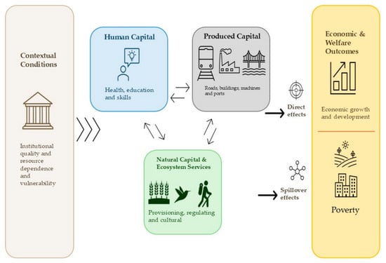
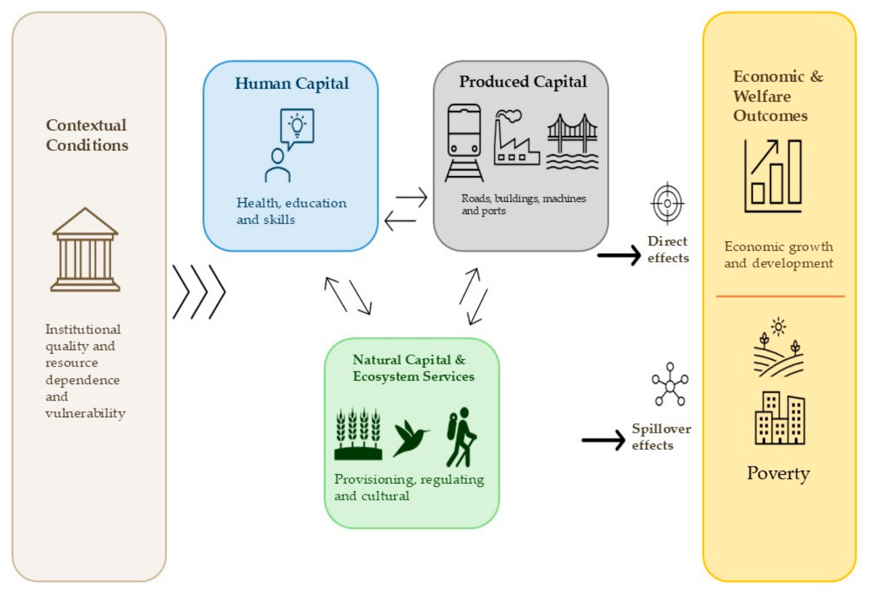
In the case of Mexico, there is a gap in the literature regarding the direct and indirect effects of natural capital on poverty. To address this gap, we draw upon Dasgupta’s [1] inclusive wealth approach and the contribution of Grammatikopoulou et al. [11] to elucidate the effect of natural capital on poverty at the municipal level and within the neighborhood of contiguous municipalities. Figure 1 provides a graphical description of the channels through which natural capital and ecosystem services can directly and indirectly affect poverty.
Figure 1.
Mediation of natural capital via ecosystem services regarding municipal poverty and municipal proximity. Source: Authors’ own elaboration, modified from Grammatikopoulou et al. [11] and Dasgupta [1].
The objective of this study is to analyze the relationship between poverty and the conservation status of remaining natural areas at the municipal level in Mexico. To address potential spatial interaction effects between these two variables, the presence of spatial dependence processes was verified, and appropriate spatial models were employed to avoid bias in the estimators measuring the relationship between poverty and natural capital. The research question guiding this work is: Is the better conservation status of remaining natural areas associated with lower levels of poverty at the municipal level and in surrounding areas? Do higher levels of natural capital within a municipality and its neighboring areas correlate with reduced poverty levels?
The methodological strategy adopted is based on a “specific-to-general” approach, which involves first estimating a non-spatial linear regression model and testing the assumption of no spatial autocorrelation in the error terms. Rejecting the corresponding null hypothesis leads to the adoption of a more general specification [16]. Based on this result, various linear spatial econometric model specifications were estimated, considering three types of spatial interaction effects: (1) endogenous interaction effects, where poverty in municipality i depends on poverty trends in municipality j; (2) exogenous interaction effects, where poverty in municipality i depends on explanatory variables from municipality j; and (3) interaction effects in the error terms, arising from a spatial interaction process among disturbances associated with omitted variables or measurement errors [17]. The empirical strategy initially involved estimating the Spatial Lag of X (SLX) model and the Spatial Durbin Error Model (SDEM); these models are characterized by their ability to estimate local indirect effects and by their relative simplicity regarding estimation and interpretation [18]. Subsequently, models capable of capturing global indirect effects were estimated, such as the Spatial Autoregressive Model (SAR), the Spatial Durbin Model (SDM), and the Spatial Autoregressive Combined Model (SAC). The results indicate that greater quantity and quality of remaining natural areas within a municipality are associated with lower poverty levels in that area. Additionally, higher quantity and quality of natural areas in adjacent municipalities are also linked to decreased poverty in the municipality.
2. Literature Review
2.1. Direct Effects of Natural Capital on Poverty
One of the first studies to analyze the relationship between poverty and the loss of remaining natural areas in the form of forest cover was conducted by Deininger and Minten [9]. The authors used a Probit model to estimate the probability of increased deforestation of forest plots in the states of Chiapas and Oaxaca during the period from 1980 to 1990. To do this, they constructed a 1 × 1 km geographic grid in 160,000 forested plots in 1980 within both States and, from this, defined the binary dependent variable that takes the value of 1 if the i-th plot (grid) changed from forest use to agricultural use during that period, and 0 otherwise. As predictor variables, they considered the incidence of poverty (percentage of the economically active population with incomes below the minimum wage), physio-geographic characteristics, types of property rights, conservation policies, and the implicit price of capital (measured by the availability of subsidized credit in the number of transactions). Among their findings, they highlighted that better access to infrastructure increases agricultural potential and, consequently, the probability of deforestation. Conversely, higher altitude and less access to paved roads decrease this probability. Likewise, high levels of poverty are associated with a greater probability of deforestation, with this relationship being more pronounced in plots with high poverty levels and less road access. Programs aimed at combating poverty by generating non-agricultural jobs in plots with less infrastructure are also linked to a lower probability of deforestation. This evidence points to a direct effect: local poverty conditions-mediated by limited access to infrastructure and non-agricultural employment-increase pressure on remaining forest cover within the same locality.
On the other hand, Khan [19] analyzed the relationship between poverty and ecological footprint in 14 Asian countries where more than 50% of the population earns less than US$1.50 per day, during the period 2010–2016. To do this, he used a panel data model with Driscoll and Kaisi (DK) estimators. His main results indicate that an increase in the ecological footprint leads to a reduction in poverty, suggesting that policies aimed at reducing environmental degradation could have positive effects on poverty levels. Since this analysis is conducted at the national level—without an explicit spatial weighting scheme—it identifies a direct structural relationship between poverty and environmental degradation, rather than the spillovers to neighboring units examined later in this work.
Similarly, Khan et al., [20] argue that the basket of goods and services on which poor households in the Khyber Pakhtunkhwa province of Pakistan depend relies 95% on natural resources available in the local forest cover. The authors used Geographic Information Systems and multivariate statistical analysis to examine the relationship between poverty and the environment, finding a strong correlation between multidimensional poverty and forest cover degradation. In this way, this pattern of dependence illustrates a direct mechanism through which the degradation of natural capital aggravates poverty: a 95% dependence on local forest resources for daily subsistence directly links household well-being with the quantity and quality of forest cover within the same locality.
2.2. Indirect and Spatial Effects of Natural, Manufactured and Human Capital on Poverty
Ntodwa and Chirwa [21] studied multidimensional spatial patterns in Malawi, using cross-sectional data from a household survey conducted in 2019 and 2020. The authors created a spatial weighting matrix based on the inverse of the distance between the centroids of the polygons that make up the clusters and applied Moran’s I statistic to analyze the spatial dependence of poverty, as well as a spatial lag regression (SAR) model. Their results indicate that 61% of the population in Malawi lives in multidimensional poverty, with this incidence being lower in urban areas compared to rural areas. Furthermore, they detected positive univariate and bivariate spatial autocorrelation processes between poverty and access to schools, which they consider a proxy for education, as well as in relation to extreme weather events. The authors found that the presence of a school within a cluster reduces multidimensional poverty both in that cluster and in nearby clusters. Likewise, extreme weather events have direct effects on the affected area and indirect effects on neighboring areas. Climate crises not only directly affect the most vulnerable communities but also generate ripple effects that impact nearby communities.
More directly related to the mechanisms examined in this study, Grammatikopou-lou et al., [9] estimated the direct and indirect effects of natural capital and its ecosystem services on regional economic growth across 222 NUTS-2 regions of the European Union. They employed a Cobb–Douglas production function using natural capital lagged by six years as an instrument to address reverse causality. Their results indicate that a 10% increase in natural capital is associated with a 0.7% rise in regional gross value added, comprising a 0.4% direct effect and a 0.3% indirect effect. Regulatory services—rather than provisioning services alone—account for the direct effect, and the spatial spillovers are geographically localized: they weaken under an inverse-distance matrix but remain robust under contiguity and k-nearest neighbor matrices, a pattern consistent with short-range ecological processes such as pollination, erosion control, and hydrological connectivity.
Overall, these lines of research leave a specific gap unaddressed: studies on deforestation and poverty [9,20] document direct effects but do not model spatial dependence; studies on multidimensional poverty [21] demonstrate both direct and indirect effects, yet focus on infrastructure and climate shocks without addressing natural capital; and the only study explicitly estimating the direct and indirect effects of natural capital [11] does so in the context of regional economic growth in the European Union, rather than municipal poverty in a developing country. This study seeks to fill that gap by estimating the direct and indirect effects of natural, manufactured, and human capital on multidimensional poverty in Mexican municipalities.
3. Materials and Methods
3.1. Data Description
Poverty is the variable corresponding to the percentage of the population living in poverty by municipality for 2020; this was obtained from CONEVAL [13]. The Natural Capital Index (NCI) at the municipal level for 2021 was obtained from vector data (*.shp) available on the geoinformation portal of the National Biodiversity Information System (SNIB) of CONABIO [10]. The Ecological integrity index (EII) was obtained from CONABIO [10]. The Gross Fixed Capital Formation (GFCF) was obtained from the 2019 Economic Census [22]. Companies measures the number of businesses in a municipality and was obtained from INEGI [23]. Education measures the percentage of the population that has completed primary, secondary, and upper secondary education. This data was obtained from the 2020 Population and Housing Census, published by the National Institute of Statistics and Geography [24]. Education2000 measures the percentage of the population with primary, secondary, and upper secondary education for the year 2000 and was obtained from CONEVAL [12]. Likewise, Table 1 presents a description of the variables along with their descriptive statistics.
Table 1.
Description of variables.
Although the agencies responsible for measuring the NCI, GFCF and Education variables do not align in their publication and measurement schedules, utilizing these variables as proxies for the capital stock enables us to estimate effects that can be interpreted as comparative static change rather than a causal relationship.
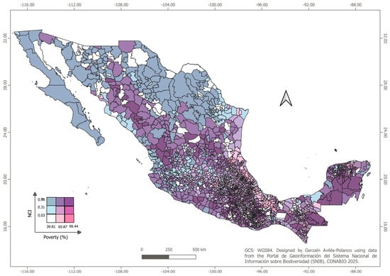
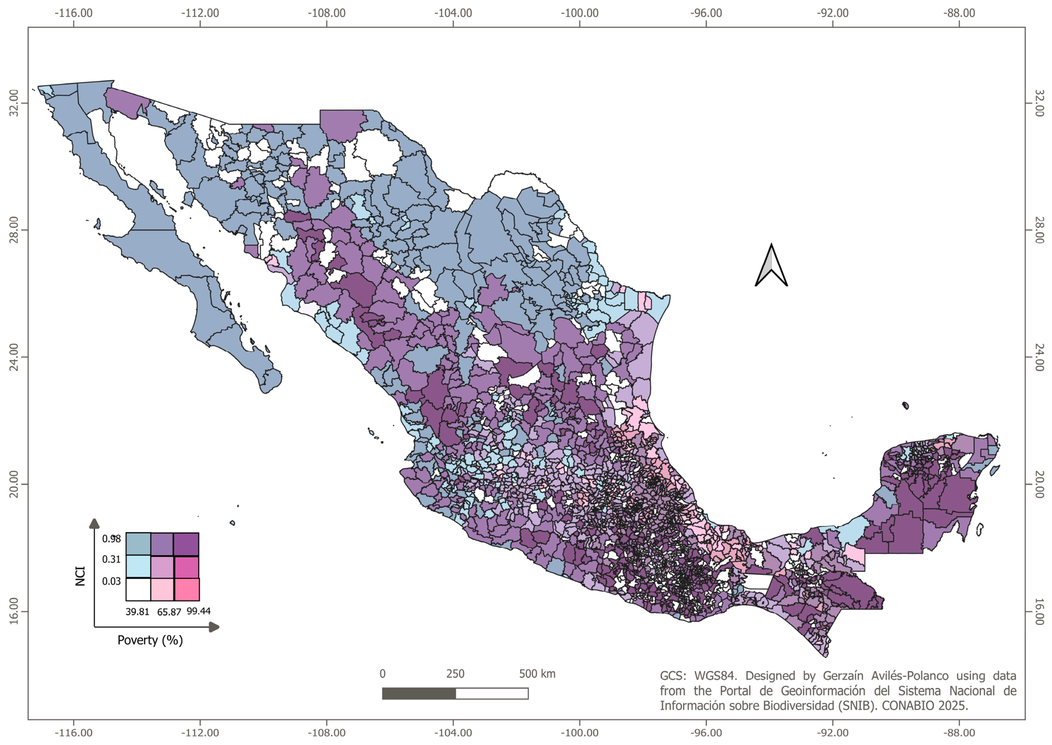
Figure 1 illustrates the spatial distribution of poverty levels and the NCI for the period 2020–2021. Three distinct patterns of bivariate spatial clustering can be observed: (a) in the regions of the Yucatán Peninsula and the western part of the country, high levels of poverty coincide with high levels of natural capital; (b) along the coastal areas of northwestern Mexico, municipalities with low poverty levels and high natural capital are evident; and (c) in the coastal zones of the Gulf of Mexico, municipalities with high poverty levels and low natural capital are observed.
The pink color on the horizontal axis represents different levels of poverty in the population, defined by the tercile cut-off points for the percentage of the population in income poverty, with darker pink indicating higher poverty. The blue color on the vertical axis represents different levels of natural resource availability, defined by the tercile cut-off points of the natural capital index. The intersection of these two gradients can be interpreted as a scatter plot. In particular, the darker areas correspond to municipalities with higher levels of poverty and a high NCI.
3.2. Spatial Autocorrelation Analysis
The global Moran’s Index statistic was used to analyze the spatial dependence of poverty and the NCI among municipalities. This statistic can be expressed as follows:
where the subscripts and denote the respective municipalities. Municipality is the one affected by an increase in natural capital in relation to poverty. Similarly, municipality also reflects the impacts on poverty stemming from increases in the natural capital of municipality . In this context, refers to a neighboring municipality. The variable x indicates the percentage of the population in income poverty at the municipal level. The elements of the matrix represent the spatial weights between municipalities, defined as:
where takes the following values:
When standardizing by row, the weight is divided by the sum of the corresponding row, denoted as . As a result, the sum of standardized weights in each row equals 1. represents the total aggregation of all spatial weights, with municipalities.
Moran’s index ranges from −1 to 1. Values greater than zero indicate positive spatial autocorrelation between poverty (NCI) at the municipal level, while values less than zero indicate negative autocorrelation between poverty (NCI) at the municipal level. A value of zero indicates no spatial correlation. The z-value is calculated using the following expression:
where
To determine whether a municipality and its neighboring municipalities form a spatial cluster, we use the Getis–Ord statistic developed by Getis and Ord [25], represented by the following formula:
where is the number of municipalities and represents the ij-th element of the spatial weights matrix with expressed as:
where is the threshold distance of the binary spatial weighting matrix . To test the statistical significance of spatial groupings we follow the development of Ord and Getis [26] and Kondo [27] to generate the z-value and p-value using the getisord command in the Stata SE-Standard edition program. The standardized values were calculated according to the following expression:
where the expected value of Getis–Ord (d) is expressed as:
With variance:
where y correspond to the sample mean and sample variance, respectively. It is assumed that the standardized distribution approximates a standard normal distribution, which allows for testing the null hypothesis regarding the existence of a random distribution of the poverty variable and natural capital assets across municipalities and their neighbors, considering a distance of 130 km.
3.3. Estimation of Instrumental Variables
Due to the endogeneity of the explanatory variables NCI, GFCF and Education, their predicted values were estimated using the Instrumental Variables (IV) method, employing the number of schools and companies as instruments in the following two-stage model:
where is a vector representing the endogenous explanatory variables (NCI, GFCF and Education), is the vector of variables used as an instrument [Education2000, Companies and Ecological Integrity Index (EII)], are the estimated values of Equation (12), and are the parameters to be estimated, and represents the random error term.
The variable Education2000, which measures the percentage of the population with primary, secondary, and high school education in the year 2000, was utilized as an instrument for the Education variable, representing the level of human capital in 2020. Additionally, the Companies variable, indicating the number of businesses per municipality, was used as an instrument for gross fixed capital formation. Similarly, the Ell variable served as an instrument for the Natural Capital Index.
3.4. General Nested Spatial Model Specification
In addition to univariate global and local autocorrelation analysis, a specific-to-general approach was used, estimating cross-sectional linear regression models with and without spatial interactions. This method allowed for the identification and comparison of the direct and indirect effects of natural capital on the population living in income poverty in Mexican municipalities. According to Elhorst [17], this approach requires estimating a non-spatial regression model and then evaluating the need to extend it to a version with spatial interactions. In this context, the specific-to-general approach for this study can be expressed through the following representations:
where is an vector of the percentage of the population living in poverty. is an vector with a value of 1 for each municipality associated with the constant term . is an matrix of variables: , , and . is an vector of parameters to be estimated, and ε is a vector of disturbance terms, independent and identically distributed with mean zero and variance . Equation was estimated using the Ordinary Least Squares (OLS) method. Subsequently, the null hypothesis , was tested using the statistical test . Rejection of the null hypothesis would indicate the need to consider a more general model that integrates various sources of spatial interaction.
According to Elhorst [17], models incorporating all types of spatial interactions were estimated. To facilitate understanding, the general nested spatial model (GNS) is initially presented in Equation (14), followed by a description of six models with fewer spatial interactions:
where is a non-negative matrix of constants that describes the type and order of spatial interactions between municipalities. represents the vector of the linear combination of the endogenous variable, which corresponds to the percentage of the population living in poverty in the vicinity of municipalities. is the matrix of spatial lags of , , and . represents the spatially lagged error variable. ρ is a spatial autocorrelation coefficient. and are vectors of parameters to be estimated that capture the direct and spatial spillover effects of the exogenous predictors. is the spatial autocorrelation coefficient. Table 2 describes the six spatial interactions added to Equation (14) and the type of spatial model by including these interactions.
Table 2.
Estimated spatial models.
3.5. Analysis of Local Effects and Spatial Spillovers
Following Arbia et al., [16] it is possible to estimate the local effect of natural capital on poverty, assuming an increase in in municipality adjacent to municipality , with total effect:
The total effect of natural capital on poverty can be divided into direct and indirect local effects. According to the development carried out by Elhorst [28], the matrix of partial derivatives of the expected value of poverty with respect to the kth explanatory variable X, related to natural, human and manufactured capital assets, is presented as follows. According to the development carried out by Elhorst [28], the matrix of partial derivatives of the expected value of poverty with respect to the kth explanatory variable , related to natural, human and manufactured capital assets, is presented as follows.
where corresponds to the element in position of matrix . From Equation (17), it follows that a change in a municipality’s will not only affect poverty within that municipality, but also impact poverty in neighboring municipalities. The effect on the municipality itself is a direct effect, represented by each diagonal element of the matrix of partial derivatives, whereas the effect on contiguous municipalities constitutes an indirect local effect, reflected in the off-diagonal elements. Stata 18.0 SE-Standard Edition software was used to estimate the models, and the data set used to ensure the reproducibility of the results is available in the Supplementary Material.
4. Results
4.1. Results of the Spatial Autocorrelation Analysis
Table 3 presents the Moran’s Index statistic values for the poverty variables, as well as for natural, human, and manufactured capital, along with the results of the statistical significance tests. Based on these results, the hypotheses of no spatial autocorrelation for all variables were rejected at the 99% confidence level, confirming the presence of positive spatial autocorrelation.
Table 3.
Moran’s Index statistics.
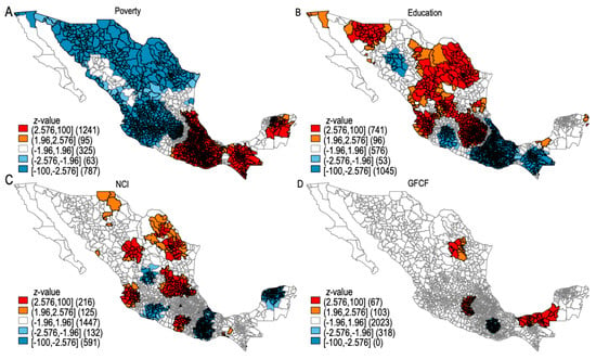
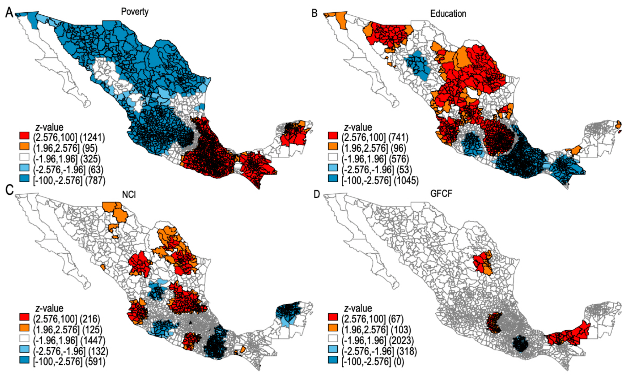
Figure 2 shows the bivariate poverty map based on income and the NCI. While the Getis–Ord statistic, calculated using a binary spatial weights matrix with a distance threshold of 130 km, identified the existence of spatial clusters in municipalities exhibiting high poverty levels surrounded by neighboring municipalities with similarly high levels, and vice versa. Figure 3 displays the spatial distribution of the Getis–Ord .
Figure 2.
Bivariate map of poverty by income and the NCI. Source: Own elaboration.
Figure 3.
Mapping Getis–Ord of poverty and natural, human, and manufactured capital assets. Source: Own elaboration.
The clusters, or hot spots, indicated by the red color gradient—corresponding municipalities with high poverty and elevated levels of natural, human, and manufacture capital—also demonstrated significance at the 99% and 95% confidence levels, with z-scores of 2.576 (p = 0.01) and 1.960 (p = 0.01), respectively. The clusters, or cold spots, represented by the blue color gradient—indicative of municipalities with low poverty and limited natural, human, and manufactured capital—were statistically significant at 99% and 95% confidence levels, with z-scores of −2.576 (p = 0.01) and −1.960 (p = 0.01) respectively.
4.2. Results of Endogeneity Tests
Before proceeding with the estimation of the direct and indirect local effects of natural capital on poverty, the presence of endogeneity derived from the inverse causality between poverty, manufactured, human and natural capital was verified. To address this issue, IV models are implemented. The results of the Two-Stage Least Squares estimates are available in Appendix A (Table A1, Table A2 and Table A3). Table 4 presents the results of the Durbin–Wu–Hausman tests and the corresponding F-statistic value of the first-stage estimate.
Table 4.
Durbin–Wu–Hausman and first-stage F-statistic test results.
The Durbin–Wu–Hausman test detected the presence of endogeneity in the NCI, GFCF, and Education variables. The first-stage F-statistic values exceeded the threshold of 10, supporting the relevance of the instruments used. Subsequently, the predicted values of these variables were incorporated into the spatial model estimations.
4.3. Results of Non-Spatial Linear Regression Models and Autocorrelation Test
A semi-logarithmic regression model was estimated using OLS method to analyze the relationship between the logarithm of the poverty variable and the , , and . Table 5 shows the results of the model estimated from Equation (14).
Table 5.
Results and diagnosis of the OLS model.
The coefficients for the variables and showed negative signs and were statistically significant at the 99% confidence level. In contrast, the coefficient for the variable showed a negative value but did not reach statistical significance at any of the conventional levels. A set of diagnostic tests were performed to detect the presence of heteroscedasticity, multicollinearity, and spatial autocorrelation. The Variance Inflation Factor (VIF) statistics indicated the absence of multicollinearity problems. The Breusch–Pagan test detected the presence of heteroscedasticity. Moran’s statistic was statistically significant, indicating positive spatial dependence. Finally, the Lagrange Multiplier tests for both errors and spatial lags were statistically significant, demonstrating the presence of spatial dependence in both the errors and lags of the lagged dependent and explanatory variables, or a combination of these sources of spatial dependence.
4.4. Results of Spatial Regression Models
The results of the non-spatial linear regression models and the spatial linear models are presented in Table 6 and Table 7.
Table 6.
Results of Spatial Linear Models OLS, SEM, SAR, and SLX.
Table 7.
Results of Spatial Linear Models SDM, SDEM, SAC and GNS.
The coefficients for the variable were negative and statistically significant at the 99% confidence level in both the non-spatial regression model and the seven linear spatial regression models, with values ranging from −0.20 to −0.09. Meanwhile, the coefficients for the variable were also negative and statistically significant at the 99% confidence level in the SLX and SMD models, with values falling within the −1.26 to −0.14 range. In the SDEM and GNS models, these coefficients remained negative and statistically significant at the 90% confidence level, with values between −0.20 and −0.18.
Regarding the (, variable, its coefficients showed negative signs and were statistically significant at the 99% confidence level in the non-spatial linear regression model, as well as in the seven spatial models (SEM, SAR, SLX, SMD, SDEM, SAC, and GNS) with values ranging from −0.03 to −0.01. The coefficients for the variable were significant at the 95% confidence level with a negative sign in the SDM, SDEM, and GNS models, with values in the −0.03 to −0.001 range. Conversely, in the SLX model, this coefficient was positive and statistically significant at the 99% confidence level, with a value of 0.004.
In the case of the variable, its coefficients showed negative signs and were statistically significant at the 99% confidence level in the SEM, SAR, SDM, SDEM, and GNS models. Likewise, the coefficients for were negative and significant at the 99% level in the SLX, SDEM, and GNS models. However, in the SDM model, this coefficient was positive and also statistically significant at the 99% confidence level.
The Pseudo R’ values presented in Table 6 and Table 7 indicate that the models with the greatest statistical fit were the SDM and GNS, both with a value of 0.37. On the other hand, the values of the AIC and BIC statistics revealed that the model that best balances fit and parsimony was the SDEM, with values of −58.61 and −6.16 respectively.
To identify the model that best explains the direct and indirect effects of natural, human, and manufactured capital assets, the Likelihood-ratio test was used. The results of the LR test are presented in Table 8.
Table 8.
Results of Likelihood-ratio test.
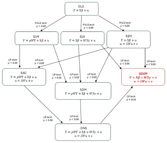
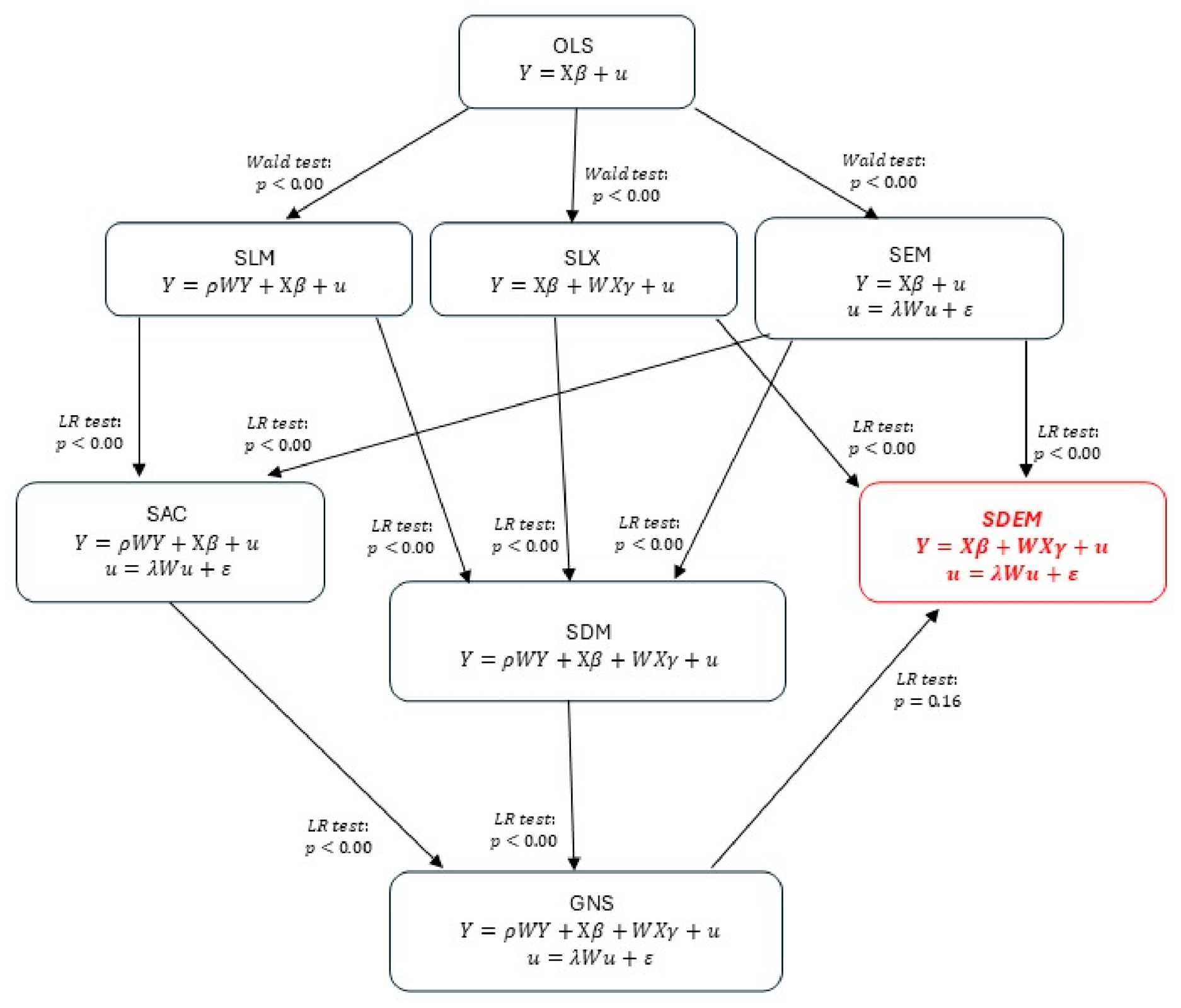
The results of the Likelihood-ratio (LR) test indicated that models with lower complexity regarding spatial interaction did not show a significant improvement in statistical fit compared to models with higher complexity (SAR vs. SAC, SAC vs. GNS, SLX vs. SDM, SDM vs. GNS, SLX vs. SDEM, and SEM vs. SDEM), with the exception of the SDEM model when compared to the GNS model.
Figure 4 illustrates the model selection directions, based on the results of the Wald and Likelihood-ratio (LR) tests, considering the levels of statistical significance at which it was not possible to reject the null hypotheses. Given that the LR test favored the SDEM model and it exhibited the lowest AIC and BIC values, the SDEM model was selected for the estimation of local direct and indirect effects.
Figure 4.
Model selection criteria based on Likelihood test results.
The local direct and indirect effects obtained from the SDEM model estimation and Equations (10) and (11) are presented in Table 9.
Table 9.
Direct and indirect effects of natural, manufactured, and social capital.
All coefficients representing the direct effects of natural, human and manufactured capital assets were found to be negative and statistically significant at the 99% confidence level. The coefficients of the variables and , which reflect the local indirect effects of human and manufactured capital on poverty, showed negative signs and a significance of 95%. On the other hand, the coefficient of the variable presented a negative sign, but its statistical significance only reached 90%. Since the dependent variable is the natural logarithm of poverty, the direct and indirect effects can be interpreted in percentage terms. On average, a 10% increase in a municipality’s natural capital is associated with an approximate 1.1% reduction in its poverty level. Although the coefficient that measures the local indirect effect was not statistically significant at the 95% level, it was significant at the 90% level, so its interpretation should be considered with caution, as weak evidence of a spatial spillover effect. Considering the above, a 10% increase in the natural capital of municipalities adjacent to a particular one is associated with a 1.3% decrease in poverty in said municipality. In relation to the total effect, a 10% increase in natural capital was found to be associated with a 2.5% reduction in regional poverty.
Regarding the local direct and indirect effects of human capital, it was observed that, on average, a 10% increase in the proportion of the population having completed primary, lower secondary, and high school in a specific municipality is associated with a 0.20% reduction in poverty within that municipality. Similarly, a 10% increase in the proportion of the population with this level of schooling in neighboring municipalities is associated with a slight reduction of 0.0008% in poverty in the municipality in question. Regarding the total effect of this variable on poverty, the average 10% increase in the proportion of the population having completed primary, lower secondary, and high school is associated with a 0.2% decrease in regional poverty.
Finally, the local direct and indirect effects of manufactured capital measured by the variable , were found to be of small magnitude. Specifically, a 10% increase in , within a given municipality corresponds to an approximate 0.00004% decrease in its poverty level. Similarly, on average, a 10% increase in this variable in neighboring municipalities is associated with around a 0.0001% reduction in poverty within the municipality in question. Additionally, a 10% increase in , is associated with a reduction in poverty by 0.00014%.
5. Discussion
The empirical results found in this study are consistent with the theoretical framework developed by Dasgupta [1], which states that poverty reduction depends on the ecological footprint of consuming environmental goods and services being less than the biocapacity of ecosystems to produce them. This is particularly relevant in regions where a significant portion of the population depends on agricultural activities susceptible to overexploitation, with limited access to markets, infrastructure, and human capital.
The results corroborate the findings of Grammatikopoulou et al. [11], who conclude that ecosystem services derived from natural capital contribute to the growth of gross value added and regional well-being. In particular, our study provides evidence that increases in natural capital are linked to an improvement in well-being, by reducing poverty in municipalities. Regarding spatial spillovers, no significant local indirect effects were found at the 95% confidence level, although they were detected at the 90% level, suggesting weak evidence of natural capital spillovers on poverty. However, the total effect of natural capital on poverty was statistically significant at the 95% confidence level, indicating that, on average, a 10% increase in natural capital is associated with a 2.5% reduction in poverty at the regional level.
Like Grammatikopoulou et al. [11], in this study we have used a contiguity matrix, considering that contiguity more accurately represents the connectivity of short-range ecosystem processes determined by orography. These processes include erosion, runoff into rivers or lakes, the capture and infiltration of water in the water tables of the basins, as well as the biological corridors (genes and species) that influence pollination and seed dispersal. In this context, estimates made using an inverse-distance matrix could lead to biased results with respect to indirect effects, since they only consider distance and not short-range ecosystem processes, influenced by orography, that give rise to the formation of bioregions.
Our results suggest that the existence of a greater number of remaining natural areas and greater ecological integrity could promote the implementation of subsistence strategies based on sustainable livelihoods, which would contribute to reducing poverty and increasing well-being at both the municipal and regional levels [15].
Our results coincide with the findings reported by Deininger and Minten [9], regarding the association of higher poverty levels with a greater likelihood of deforestation. This study provides evidence of a direct and indirect negative association between natural capital and poverty. The channels through which an increase in remaining natural areas and their ecological integrity is related to lower poverty may be due to greater access to markets and less dependence on agricultural jobs, as indicated by Deininger and Minten [9]. While these results reveal effects through direct and indirect associations, further studies are needed with a causal effect analysis approach. Such studies should consider interventions like ecosystem restoration programs and the promotion of non-agricultural employment, comparing outcomes between municipalities with and without these interventions while controlling for covariates to avoid confounding factors.
In municipalities with higher poverty levels natural capital conservation policies should include interventions such as employment programs that are not directly tied to agricultural activities. These municipalities are characterized by a high dependence on natural resources within their local forest cover, which favors deforestation, as noted by Khan et al. [20]. Such approaches could also lead to positive indirect effects on poverty alleviation, as evidenced by our findings.
In relation to the direct and indirect effects of human capital on poverty, our results are consistent with the reports of Ntodwa and Chirwa [21], who point out that greater access to education, facilitated through educational infrastructure, is associated with a reduction in poverty levels both in the district with schools and in neighboring districts. In our study, it was found that an increase in the percentage of the population with completed primary, secondary and high school studies in a specific municipality is related to a decrease in poverty in said municipality. Likewise, an increase in natural capital in the vicinity of municipalities adjacent to a particular municipality is also associated with a reduction in poverty in that municipality.
Regarding the direct and spillover effects of manufactured capital on poverty, our results coincide with the findings of Deininger and Minten [9], who analyzed the relationship between poverty and the loss of forest cover, finding that high levels of poverty are associated with a greater probability of deforestation, especially in areas with less access to road infrastructure. Unlike Deininger and Minten [9], who used access to roads as a manufactured capital variable, in our study we use the , variable as a proxy for manufactured capital. However, both studies agree that an increase in manufactured capital is directly related to lower levels of poverty. Furthermore, our analyses reveal the existence of negative and statistically significant spatial spillover effects of manufactured capital on poverty.
6. Conclusions
This study used cross-sectional data related to poverty and social, human, and manufactured natural capital to analyze the direct and indirect effects of natural capital on poverty in municipalities in Mexico. It also evaluated the spatial spillover effects of natural, human and manufactured capital on poverty, specifically how natural capital index, education and gross fixed capital formation in neighboring municipalities influence poverty levels in one municipality. Moran’s indices and Moran’s test were used on the residuals of a model estimated using the OLS method. Based on these analyses, spatial linear models were specified and estimated, including SEM, SAR, SLX, SDEM, SDM, SAC and GNS models. These models were then subjected to various statistical tests, such as the Wald test and the LR test.
Likelihood-ratio test results indicated that the SDEM model—which entails less complexity regarding spatial interactions compared to the GNS model—was selected to estimate local direct and indirect effects.
Furthermore, the findings showed that a 10% increase in natural capital is associated with a 2.5% decrease in regional poverty. Conversely, a 10% increase in the share of the population with primary, secondary, and high school-level education is linked to a 0.20% reduction in regional poverty. Finally, a 10% increase in gross fixed capital formation is associated with a very slight decrease of 0.00014% in regional poverty.
The main limitation of this study is that models estimated with cross-sectional data do not capture the unobserved and time-invariant heterogeneity specific to each municipality. Therefore, spatial panel data models are needed in future studies. Nevertheless, we believe this study contributes information into the direction and magnitude of the relationship between poverty and natural capital, which will serve as a reference for future research.
This study enhances the existing literature on the impact of natural capital on poverty by identifying a negative correlation between natural capital and the proportion of the population experiencing poverty in Mexican municipalities. Additionally, the research reveals a negative relationship between human capital and poverty levels within these regions. Furthermore, evidence indicates a negative association between manufactured capital and the percentage of the population living in poverty.
These findings have important implications for the design of public policies aimed at combating poverty and conserving natural capital in Mexico. Poverty reduction programs must consider the spatial interrelationship and feedback loops between available natural resources and the unmet needs of the most vulnerable populations. Manufactured and human capital are fundamental elements for achieving levels of economic development that reduce dependence on resources available in forest cover, as well as land-use change and defaunation.
Supplementary Materials
The following supporting information can be downloaded at https://www.mdpi.com/article/10.3390/geographies6030095/s1. Spreadsheet containing the datasets used for model estimation and statistical testing. manuscript-supplementary.xlsx.
Author Contributions
Conceptualization and design of study: G.A.-P. and L.F.B.-M. Acquisition of data, curation, and software: G.A.-P. and L.S. Analysis and/or interpretation of data: G.A.-P., L.F.B.-M., L.S. and D.A.R.-F. Drafting the manuscript: G.A.-P. and L.F.B.-M., L.S., L.R.-T. and D.A.R.-F. Review and editing: L.S. and L.R.-T. All authors have read and agreed to the published version of the manuscript.
Funding
This research was funded by the Secretaría de Ciencia, Humanidades Tecnología e Innovación (SECIHTI), through the project CBF 2023-2024-4308: “Efectos directos e indirectos del capital natural y social sobre la pobreza por ingreso y capacidades”.
Institutional Review Board Statement
Not applicable.
Informed Consent Statement
Not applicable.
Data Availability Statement
The original contributions presented in this study are included in the article/Supplementary Material. Further inquiries can be directed to the corresponding author.
Acknowledgments
We thank the Centro de Investigaciones Biológicas del Noroeste (CIBNOR) for supporting the completion of this research.
Conflicts of Interest
The authors declare no conflicts of interest.
Abbreviations
The following abbreviations are used in this manuscript:
| CONABIO | National Commission for the Knowledge of Biodiversity |
| CONEVAL | National Council for the Evaluation of Social Development Policy |
| INEGI | National Institute of Statistics and Geography |
| NCI | Natural Capital Index |
| GFCF | Gross Fixed Capital Formation |
| LR | Likelihood Ratio |
| VIF | Variance Inflation Factor |
| AIC | Akaike’s Information Criteria |
| BIC | Bayesian Information Criterion |
| OLS | Ordinary Least Squares |
| SAR | Spatial Autoregressive Model |
| SEM | Spatial Error Model |
| SLX | Spatial Lag Model of X |
| SAC | Spatial Combined Autoregressive Model |
| SDM | Spatial Durbin Model |
| SDEM | Spatial Durbin Error Model |
| GNS | General Nested Spatial Model |
Appendix A
Table A1.
Poverty estimation results using instrumental variables. Instrument: EII.
Table A2.
Poverty estimation results using instrumental variables. Instrument: Companies.
Table A3.
Poverty estimation results using instrumental variables. Instrument: Education2000.
References
- Dasgupta, P. The Economics of Biodiversity: The Dasgupta Report; HM Treasury: London, UK, 2021; pp. 1–604. [CrossRef] [Scilit]
- Costanza, R.; de Groot, R.; Sutton, P.; van der Ploeg, S.; Anderson, S.J.; Kubiszewski, I.; Farber, S.; Turner, K.R. Changes in the Global value of Ecosystem services. Glob. Environ. Change 2014, 26, 152–158. [Google Scholar] [CrossRef] [Scilit]
- Dasgupta, P. Getting India Wrong. Prospect 2013. Available online: https://www.prospectmagazine.co.uk/culture/51266/getting-india-wrong (accessed on 24 February 2026).
- Hamann, M.; Berry, K.; Chaigneau, T.; Curry, T.; Heilmayr, R.; Henryksson, P.J.G.; Hentati-Sundberg, J.; Jina, A.; Lindkvist, E.; Lopez- Maldonado, Y.; et al. Inequality and the Biosphere. Annu. Rev. Environ. Resour. 2018, 43, 61–83. [Google Scholar] [CrossRef] [Scilit]
- Schaafsma, M.; Morse-Jones, S.; Posen, P.; Swetnam, R.D.; Balmford, A.; Bateman, I.J.; Burgess, N.; Chamshama, S.; Fisher, B.; Freeman, T.; et al. The Importance of Local Forest Benefits: Economic Valuation of Non-Timber Forest Products in the Eastern Arc Mountains in Tanzania. Glob. Environ. Change 2014, 24, 295–305. [Google Scholar] [CrossRef] [Scilit]
- Schaafsma, M.; Fisher, B. What are the Links Between Poverty and Ecosystem Services? In Routledge Handbook of Ecosystem, 1st ed.; Potschin, M., Haines-Young, R., Fish, R., Turner, R.K., Eds.; Routledge: New York, NY, USA, 2016; pp. 1–11. [Google Scholar] [CrossRef] [Scilit]
- Czucz, B.; Molnar, Z.; Horvarth, F.; Nagy, G.; Botta-dukat, Z.; Torok, K.; Schaafsma, M. Using the natural capital index framework as a scalable aggregation methodology for regional biodiversity indicators. J. Nat. Conserv. 2012, 20, 144–152. [Google Scholar] [CrossRef] [Scilit]
- Mora, F. The use of ecological integrity indicators within the natural capital index framework: The ecological and economic value of the remnant natural capital of Mexico. J. Nat. Conserv. 2019, 47, 77–92. [Google Scholar] [CrossRef] [Scilit]
- Deininger, K.; Minten, B. Determinants of Deforestation and the Economics of Protection: An Application to Mexico. Am. J. Agric. Econ. 2022, 84, 943–960. [Google Scholar] [CrossRef] [Scilit]
- Comisión Nacional para el Conocimiento y Uso de la Biodiversidad (CONABIO), Índice de Capital Natural. Portal de Geo-Información. 2021. Available online: http://www.conabio.gob.mx/informacion/gis/ (accessed on 14 February 2026).
- Grammatikopoulou, I.; Giannakis, E.; Maes, J.; Nucci, M.Z. Spillover effects of natural capital: Implications for regional development and cohesion policy in the European Union. Reg. Sci. Policy Pract. 2026, 18, 100314. [Google Scholar] [CrossRef] [Scilit]
- CONEVAL Consejo Nacional de Evaluación de la Política de Desarrollo Social. Medición multidimensional de la pobreza en México. Trimes. Econ. 2014, 81, 5–42. Available online: https://www.eltrimestreeconomico.com.mx/index.php/te/article/view/151/342 (accessed on 12 February 2026).
- Consejo Nacional de Evaluación de la Política de Desarrollo Social (CONEVAL). Resultados de Pobreza en México 2022 a Nivel Nacional y por Entidades Federativas. 2022. Available online: https://www.coneval.org.mx/Medicion/Paginas/PobrezaInicio.aspx (accessed on 12 January 2026).
- Sen, A. The possibility of Social Choice. Am. Econ. Rev. 1999, 89, 349–378. Available online: https://www.aeaweb.org/articles?id=10.1257/aer.89.3.349 (accessed on 12 January 2026). [CrossRef] [Scilit]
- Serrat, O. The Sustainable Livelihoods Approach. In Knowledge Solutions; Springer: Singapore, 2017. [Google Scholar] [CrossRef] [Scilit]
- Arbia, G. A Primer for Spatial Econometrics with Applications in R; Springer: Berlin/Heidelberg, Germany, 2014; pp. 1–631. [Google Scholar] [CrossRef] [Scilit]
- Elhorst, J.P. Spatial panel models and common factors. In Handbook of Regional Science; Fischer, M., Nijkamp, P., Eds.; Springer: Berlin/Heidelberg, Germany, 2019; Available online: https://link.springer.com/rwe/10.1007/978-3-662-60723-7_86 (accessed on 12 January 2026).
- Halleck Vega, S.; Elhorst, J.P. The SLX Model. J. Reg. Sci. 2015, 55, 339–363. [Google Scholar] [CrossRef] [Scilit]
- Khan, S.U.D. Environmental sustainability: A clean energy aspect versus poverty. Environ. Sci. Pollut. Res. 2021, 28, 13097–13104. [Google Scholar] [CrossRef] [Scilit] [PubMed]
- Khan, I.; Saqib, M.; Hafidi, H. Poverty and environmental nexus in rural Pakistan: A multidimensional approach. GeoJournal 2021, 86, 663–677. [Google Scholar] [CrossRef] [Scilit]
- Ntodwa, E.; Chirwa, G.C. Spatial spillover effect of multi-dimensional poverty in Malawi. Humanit. Soc. Sci. Commun. 2025, 12, 1447. [Google Scholar] [CrossRef] [Scilit]
- INEGI. Censos Económicos 1999, 2009 y 2019. 2023. Available online: https://www.inegi.org.mx/programas/ce/2019/ (accessed on 15 January 2026).
- INEGI. Directorio Estadístico Nacional de Unidades Económicas (DENUE). Available online: https://www.inegi.org.mx/app/mapa/denue/default.aspx (accessed on 11 January 2026).
- INEGI. Grado Promedio de Escolaridad de la Población de 15 y más años por Entidad Federativa Según Sexo, años Censales Seleccionados 2000 a 2020. 2023. Available online: https://www.inegi.org.mx/app/tabulados/interactivos/?pxq=Educacion_Educacion_05_d80252d5-9779-4ff4-a336-d5dd3f717588 (accessed on 23 January 2026).
- Getis, A.; Ord, J.K. The Analysis of Spatial Association by Use of Distance Statistics. Geogr. Anal. 1992, 24, 189–206. [Google Scholar] [CrossRef] [Scilit]
- Ord, J.K.; Getis, A. Local Spatial Autocorrelation Statistics: Distributional Issues and an Application. Geogr. Anal. 1995, 27, 286–306. [Google Scholar] [CrossRef] [Scilit]
- Kondo, K. Hot and Cold Spot Analysis Using Stata. Stata J. Promot. Commun. Stat. Stata 2016, 16, 613–631. [Google Scholar] [CrossRef] [Scilit]
- Elhorst, J.P. Spatial Econometrics: From Cross-Sectional Data to Spatial Panels; Springer: Berlin/Heidelberg, Germany, 2014; Volume 479, p. 480. [Google Scholar] [CrossRef] [Scilit]

Disclaimer/Publisher’s Note: The statements, opinions and data contained in all publications are solely those of the individual author(s) and contributor(s) and not of MDPI and/or the editor(s). MDPI and/or the editor(s) disclaim responsibility for any injury to people or property resulting from any ideas, methods, instructions or products referred to in the content. |
© 2026 by the authors. Licensee MDPI, Basel, Switzerland. This article is an open access article distributed under the terms and conditions of the Creative Commons Attribution (CC BY) license.