


Abstract
Rapid urban population expansion in semi-arid environments poses considerable challenges for sustainable planning, particularly where demographic growth occurs under environmental constraints. This study examines the statistical association between climatic variability and population change in the Soran district center, Kurdistan Region of Iraq, and develops an exploratory framework for forecasting future demographic trends. It uses the official annual population series compiled by the Statistics Directorate of the Soran Independent Administration for 2010–2024 (15 observations) together with monthly meteorological records for 2015–2024 from the Soran agro-meteorological station. Two properties of the demographic record govern what can be inferred from it. The 2010–2023 values are inter-censal estimates reproduced to within 0.10% by a single declining-growth rule, so goodness-of-fit statistics obtained on that segment measure agreement with an interpolation rule rather than forecasting skill; and the 2024 value derives from the 2024 census round, representing a level shift of +18.4% against a 2.0% per year trend—178 residual standard deviations—rather than a year of growth. Detrended, lagged Spearman correlations across twelve climate–lag combinations yielded no association surviving Holm–Bonferroni correction; because the pre-2024 values are administratively smoothed, this is reported as an inability of the available data to resolve a climate–demography association rather than as evidence of independence. Eight specifications—naïve, drift and linear-trend benchmarks, a second-order polynomial, a log-linear trend, an AIC-selected ARIMA, and two multilayer perceptrons—were compared under identical rolling-origin cross-validation, producing seven one-step-ahead forecasts each. On the inter-censal segment a random walk with drift attained a mean absolute percentage error of 0.087%, better than every fitted specification; on the census fold every specification erred by at least 11,663 persons. The reported 2025–2030 projection is therefore anchored on the 2024 census level with growth extrapolated from its 2011–2023 trend, giving 93,342 residents in 2025 and 101,691 in 2030 (scenario range 100,395–104,064), reproduced to within 488 persons by an ARIMA(0,2,2) with a 2024 step term. Polynomial and log-linear trends fitted across the discontinuity project 2025 values are below the observed 2024 population and are reported as specification failures. The study demonstrates both the potential and the limitations of demographic forecasting in data-scarce semi-arid urban settings and shows that the provenance of an administrative population series materially constrains the claims such a study can make.
1. Introduction
Urbanization represents a pivotal demographic transformation of the twenty-first century, with United Nations projections estimating that 68% of the global population will reside in urban areas by 2050 [1]. In semi-arid territories, rapid urban development severely strains environmental carrying capacity, particularly in relation to water infrastructure and agricultural sustainability [2,3]. The relationship has traditionally been viewed through environmental determinism, in which climate directly dictates human settlement patterns [4], and paleodemographic work does document climate-driven cycles of demographic expansion and contraction over multi-century timescales [5]. At the short, recent timescales relevant to municipal planning, however, socio-economic drivers such as employment opportunities and regional infrastructure may act as primary pull factors, potentially reducing the dependence of population expansion on local environmental limits [6,7]; whether this applies to Soran is an empirical question this study investigates rather than assumes.
Testing whether short-term population growth is statistically associated with local hydro-climatic variability is therefore relevant for understanding demographic change in semi-arid urban centers [8,9]. Conversely, where climate variability does constrain growth, forecasting models that ignore this relationship risk systematic bias [10]. Despite this policy relevance, empirical studies linking climate dynamics with demographic change in small and secondary urban centers remain comparatively limited, as much of the urban climate literature has historically focused on large cities and metropolitan areas [11,12].
In the Kurdistan Region of Iraq, previous geographic and urban studies have relied heavily on remote sensing and GIS to analyze spatial sprawl and land-use change (e.g., [13,14]). However, existing studies of the Soran territory have predominantly focused on land-cover transformations, geomorphological features, or broader regional ecosystem assessments, while largely overlooking quantitative demographic forecasting and its relationship with local climate variability. As Soran rapidly evolves into a primary economic and administrative hub in northern Iraq, this reliance on spatial assessments alone leaves a critical planning gap.
Accurate demographic forecasting is crucial for sustainable resource allocation [15]. Traditional time-series models such as ARIMA can incorporate exogenous trend and structural-break terms [16], while demographic outcomes are known to respond non-linearly to environmental and socio-economic pressure [17,18], which has motivated the application of machine-learning architectures such as Multi-Layer Perceptrons (MLPs) to population dynamics. Their data requirements and extrapolation behavior nevertheless warrant careful evaluation in data-scarce settings: ReLU networks converge to linear behavior outside the convex hull of their training inputs, so their out-of-range forecasts are governed by the architecture rather than by the data [19] (Section 2.7). Beyond its substantive findings for Soran, this study’s methodological contribution—a rolling-origin validation protocol, an explicit diagnosis of the provenance of the demographic series, and a treatment of census rebasing as a level shift, suited to short annual demographic series (here N = 15)—is intended to generalize to other rapidly urbanizing, data-scarce administrative centers where similar forecasting and data-quality challenges arise.
To address this knowledge gap, this study pursues four objectives:
- Assess the statistical relationship between demographic growth and climate variability in Soran, and establish what the provenance of the available population series permits that relationship to demonstrate.
- Develop a comparative forecasting framework merging econometric and deep learning methods.
- Evaluate the out-of-sample forecast accuracy of the candidate specifications—a second-order polynomial trend, a log-linear trend, an AIC-selected ARIMA, and two Multi-Layer Perceptron architectures—against naïve, drift and linear-trend benchmarks under an identical rolling-origin validation scheme in a data-scarce context.
- Discuss the resource-planning implications of the estimated population trajectory for semi-arid regional planning. No water-demand, groundwater, supply-capacity or resource-balance model is estimated here; the discussion identifies planning considerations and research needs rather than quantifying resource outcomes.
2. Materials and Methods
To evaluate the potential relationship between demographic dynamics and meteorological parameters, a non-parametric method was employed. Because environmental and population data frequently exhibit non-linear distributions and contain outliers, Spearman’s rank correlation coefficient (ρ) was used instead of Pearson’s correlation coefficient. The test is applied to detrended year-on-year growth rates of the annual population series against annual climate aggregates—never to an interpolated monthly population series—at lags of 0, 1 and 2 years for four climate variables. Statistical significance was assessed at the 95% confidence level (α = 0.05), with Holm–Bonferroni and Benjamini–Hochberg adjustments reported alongside raw p-values because twelve tests are performed.
2.1. Study Area
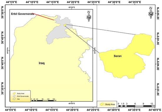
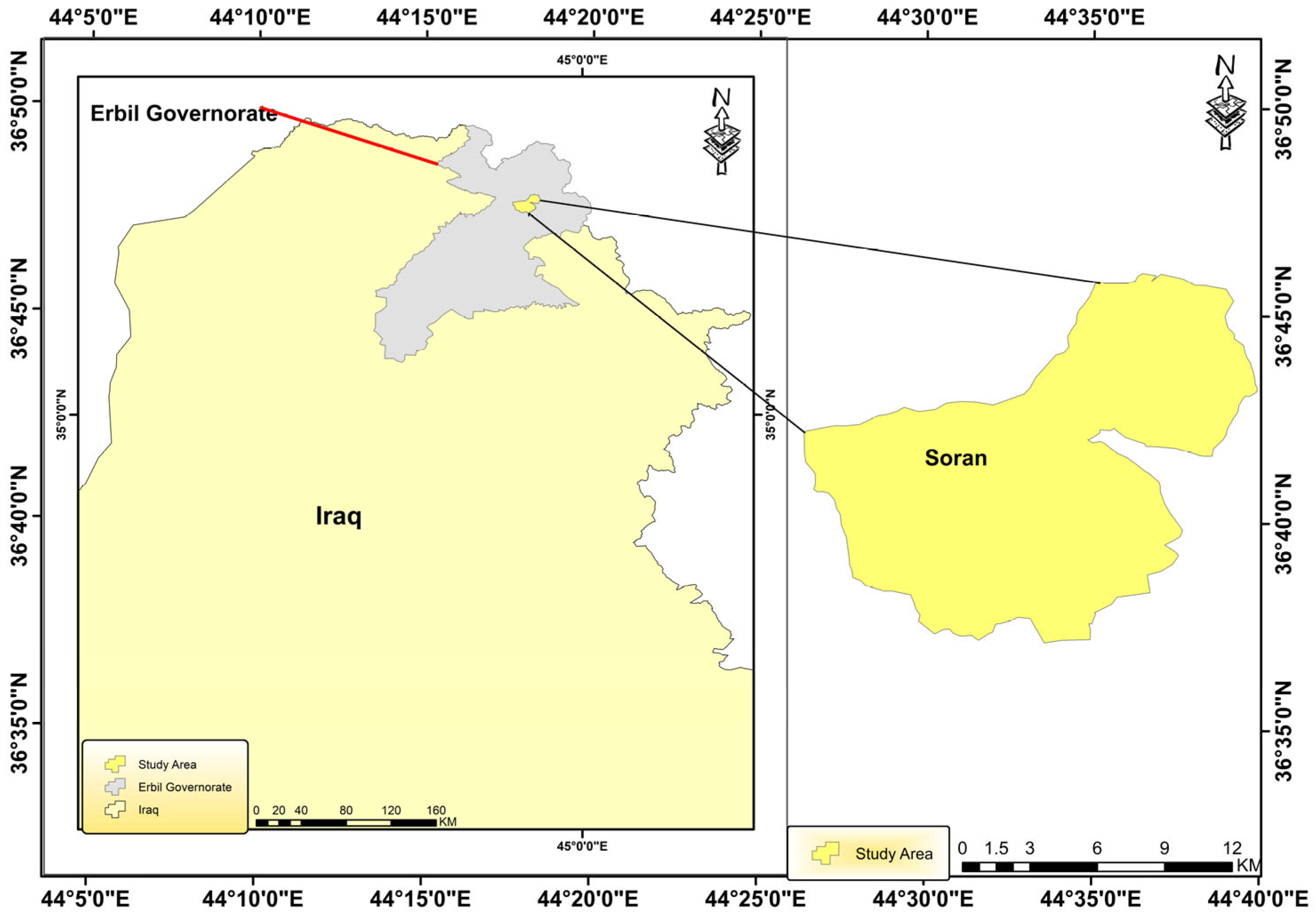
This research focuses on the Soran area, situated in the Erbil Governorate of the Kurdistan Region of Iraq [14]. Soran is located in a mountainous, semi-arid climatic area characterized by strong seasonal rainfall and substantial temperature variability (Figure 1). The administrative area of the district center is 2135 km2. Over the past two decades, the study area has experienced rapid urban growth, driven by its strategic position as a regional economic hub and its proximity to popular mountainous tourism destinations. A combination of economic development, rural-to-urban migration, and residential infrastructure expansion has fueled population growth in Soran [13]. Climatically, the district exhibits a transitional Mediterranean–continental climate, characterized by wet winters and dry summers. Over the 2015–2024 station record analyzed here, annual precipitation ranged from 485 mm (2021) to 1070 mm (2018), with a mean of 765 mm, and mean annual temperature ranged from 18.06 °C (2023) to 20.09 °C (2024); most precipitation falls between November and April [20].
Figure 1.
Geographical Location of the Soran Study Area.
Consequently, understanding the interaction between hydrological constraints and demographic expansion is critical to achieving sustainable urban development in the area.
2.2. Data Sources, Provenance, and Preprocessing
The demographic input is the official annual population series for the Soran district center (Naewendî Soran) compiled by the Statistics Directorate of the Soran Independent Administration, covering 2010–2024: 15 annual observations rising from 56,761 to 91,589 persons. The source documentation states that the 2010–2023 figures are estimates obtained by applying an estimated percentage growth rate to the 2009–2010 building-and-population enumeration, while the 2024 figure derives from the 2024 population and housing census round, which recorded 179,596 persons for the Soran district as a whole. The two segments are therefore produced by different instruments and are not comparable year-on-year, a point developed in Section 2.3 and Section 3.1. Population density is obtained by dividing population by the administrative area of 2135 km2 and is a deterministic rescaling carrying no additional information. The meteorological input is the Soran agro-meteorological station log (36°39′ N, 44°32′ E, 680 m a.s.l.) for 2015–2024, comprising 120 station-months. Given the length of the annual series, a rolling-origin (expanding-window) cross-validation scheme was adopted instead of a single fixed train–test split. At each forecast origin, the model was trained on all observations up to that year and used to forecast the subsequent year, resulting in seven one-step-ahead validation folds:
- Train 2010–2017 → forecast 2018;
- Train 2010–2018 → forecast 2019;
- Train 2010–2019 → forecast 2020;
- Train 2010–2020 → forecast 2021;
- Train 2010–2021 → forecast 2022;
- Train 2010–2022 → forecast 2023;
- Train 2010–2023 → forecast 2024.
Each fold produced one out-of-sample forecast error. The seven errors obtained for each model were aggregated to characterize forecasting performance and are additionally reported for the six inter-censal folds alone, because the 2024 fold tests a census rebasing rather than a year of demographic change. Because only seven forecast origins are available, the resulting error estimates should be interpreted as indicative rather than asymptotically stable.
To provide regular temporal inputs for the neural network models, the annual training data were temporally upsampled to monthly frequency using cubic-spline interpolation. This procedure was applied only within the training portion of each rolling-origin fold and was refitted using the observations available up to that forecast origin, so no information from the held-out forecast year entered the interpolation. The interpolated series is used solely as an input-shaping device for the multilayer perceptrons: it enters no hypothesis test, no correlation analysis and no reported accuracy statistic, and it does not imply that sub-annual demographic observations were available.
For the MLP, input and output values were scaled separately within each training fold using a standard MinMaxScaler (feature range [0, 1], the scikit-learn default), fit exclusively on that fold’s training data to prevent information leakage. The same fold-specific scaler was then applied to the corresponding validation observation.
Forecast accuracy was assessed using the Mean Absolute Percentage Error (MAPE), Mean Absolute Error (MAE), Root Mean Square Error (RMSE) and out-of-sample R2. Pairwise model comparisons used the Diebold–Mariano (DM) test [21] with squared-error loss and the Harvey–Leybourne–Newbold small-sample correction [22], given the limited number of independent forecast errors. Forecasting skill was benchmarked against three deliberately simple alternatives evaluated under the identical rolling-origin protocol—a naïve last-observation forecast, a random-walk-with-drift model, and a simple OLS linear trend—with performance also expressed as the Mean Absolute Scaled Error (MASE) [23], scaled by the mean one-step naïve absolute error inside each fold’s own training window, and as the ratio of each model’s mean absolute error to that of the naïve benchmark (RelMAE). Fold-level absolute errors are reported individually because aggregate statistics computed from seven forecast targets are unstable. For the 2025–2030 projection, uncertainty is expressed as an explicit scenario range over the assumed growth rate rather than as a residual-resampling prediction interval; Section 2.8 explains why residual-based intervals are not credible for this series.
The complete preprocessing and validation procedure was therefore performed separately for each rolling-origin fold, ensuring that interpolation, normalization, model fitting, and evaluation were conducted without information leakage from future observations.
Before aggregation, the monthly station log was screened with a documented quality-assurance protocol because the record contains transcription artifacts that a missing-value check does not detect. Six rules were applied: violation of the physical ordering min ≤ mean ≤ max within a month (R1); runs of three or more consecutive identical values in a column, indicating a filled-down cell, with exact zeros in precipitation exempt (R2); a mean monthly diurnal range exceeding 25 °C (R3); a value deviating from its month-of-year median by more than four scaled median absolute deviations, applied to temperature variables only (R4); pan evaporation below 20% of the month’s climatology, indicating an instrument out of service (R5); and values outside physical range (R6). Rules R1, R2, R3, R5 and R6 identify values that are physically impossible or demonstrably artefactual, and the affected cells were removed and imputed with the month-of-year median across the remaining years, which preserves the seasonal cycle where linear interpolation across adjacent months would not. R4 is a statistical screen that flags values for review without altering them so that genuine climate extremes are not deleted. Of 75 flagged cells, 57 were corrected and 18 retained with a flag; all are listed with their original values in the supplementary quality-assurance log (Table S2).
Three clusters account for most of the corrections. In 2016 the maximum-temperature column is filled down with the constant 16.0 °C from April to December, which places the monthly maximum below the monthly mean for seven months; uncorrected, this depresses the 2016 mean annual maximum by approximately 10 °C. In 2020, June to September carry a block of repeated placeholder values across five variables together with summer minima near 8 °C, implying a diurnal range above 31 °C. In 2023, the evaporation pan records 0.9–7.3 mm per month from January to August against a July norm near 280 mm, indicating an instrument outage; uncorrected, the 2023 annual evaporation total is about one-fifth of its corrected value. Monthly climate data were then aggregated to the annual scale as the mean of monthly temperature and humidity values and the sum of monthly precipitation and evaporation values for each year. No additional detrending was applied to the annual climate variables.
2.3. Analysis of Serial Dependence and Stationarity
To identify an appropriate modeling strategy, the stochastic properties of the series were evaluated using the autocorrelation function (ACF), partial autocorrelation function (PACF), and Augmented Dickey–Fuller (ADF) unit-root test. Because population is recorded annually while temperature and precipitation are recorded monthly, each ADF test is applied at its own native resolution (population: n = 15 annual values; climate variables: n = 120 monthly values); results across variables are therefore not comparable in test power and should not be interpreted as testing the same underlying temporal process. The population series is additionally tested in first differences and in growth rates because its level is dominated by a deterministic administrative growth rule (Section 3.1). No population autocorrelation function is reported: fifteen annual observations are too few to estimate one, and the population ACF shown in the previous version of this manuscript was computed on a spline-interpolated monthly series and therefore described the interpolation rather than the population.
2.4. Feature Selection and Model Framing
Mean monthly temperature, total precipitation, mean relative humidity and total pan evaporation were assessed as candidate exogenous predictors of population change. Bivariate correlation analysis (Spearman’s ρ) was computed on the annual series over the 2015–2024 climate–population overlap (n = 10 years; 9 growth-rate pairs), with both series detrended before testing, at lags of 0, 1 and 2 years—twelve variable–lag combinations in total. Because twelve tests are performed, raw p-values are reported alongside Holm–Bonferroni [24] and Benjamini–Hochberg false-discovery-rate [25] adjustments. One combination reached nominal significance (humidity at lag 0, ρ = 0.78, p = 0.013) but did not survive correction (Holm–Bonferroni p = 0.150); no other combination approached significance. Given this result, and given that the pre-2024 population values are administratively smoothed and therefore carry no independent year-to-year demographic signal, no meteorological variable was retained as a predictor in the population forecasting models.
Gross domestic product (GDP) and housing-unit availability were initially considered as candidate socio-economic regressors. However, no independently observed annual records of local GDP, housing completions, employment, or migration were available for the study area during 2010–2024. The proxies initially constructed for these variables—housing stock derived by dividing population by an assumed average household size (5.1 individuals, KRSO 2017 baseline) and local GDP derived by indexing population against national GDP per capita growth—are direct mathematical transformations of the population series and therefore cannot serve as independent or genuinely exogenous predictors. Including them in the forecasting models would mechanically inflate apparent forecasting accuracy without providing independent socio-economic information, because the predictors are deterministic functions of the target variable.
Both proxies were therefore excluded from all forecasting models. The population forecasting task is instead framed as a univariate trend-extrapolation exercise using only the historical population series as input. In the present revision, the leaky-diagnostic comparison reported previously has also been withdrawn, together with the Vector Autoregression specification that depended on it (Section 2.5.1), because it cannot be evaluated against the corrected data without reintroducing the circular predictors it was intended to characterize. Genuinely independent socio-economic indicators, such as employment records, housing-completion permits, or migration statistics, were not available for the study area and period; incorporating such variables is identified as a direction for future work.
2.5. Model Architectures and Configurations
Eight specifications were evaluated under identical rolling-origin cross-validation. Three are deliberately elementary benchmarks: a naïve last-observation carry-forward, a random walk with drift, and an ordinary least squares linear trend on year. Two are deterministic trend functions fitted to the population level: a second-order polynomial in year and a log-linear (constant-growth) trend. One is a stochastic time-series model: an ARIMA whose (p, d, q) order is selected by AIC grid search with the seasonal order fixed at (0, 0, 0, 0), since an annual series has no sub-annual frequency and no seasonal term is estimable—the specification is therefore correctly reported as an ARIMA(X), not a SARIMAX. Two are Multi-Layer Perceptrons: the 128 × 128 × 128 architecture of the original submission (ReLU activation, Adam optimizer, initial learning rate 0.001, L2 penalty 0.001, random seed 42) and a small, heavily regularized 8 × 8 alternative (L2 penalty 0.1), both fitted on a fold-internal cubic-spline monthly upsample of the training years. A ninth construction, the growth-rate projection anchored on the 2024 census level, is used for the final forecast only and is described in Section 2.8; it has no free parameters to validate out of sample. The Vector Autoregression specification of the previous version has been withdrawn (Section 2.5.1).
2.5.1. Vector Autoregression (VAR)—Withdrawn in This Revision
In the previous version, VAR was reported only as a diagnostic baseline, fitted with the population-derived GDP and housing proxies described in Section 2.4. Because those proxies are direct mathematical transforms of population, the specification could not produce valid demographic predictions, and its reported instability characterized the circularity of its inputs rather than any property of the population series. It has therefore been removed from the present analysis rather than recomputed on the corrected data, and no VAR results are reported.
2.5.2. ARIMA with a Census Level-Shift Term
Population was modeled as a univariate series with a single exogenous term: a step indicator taking the value 0 before 2024 and 1 from 2024 onward, representing the census rebasing identified in Section 3.1. The linear time trend and the 2023 level-shift indicator used in the previous version are not retained: on the corrected series there is no 2023 break, and the differencing order selected by AIC already accommodates the trend. No GDP or housing terms are included, consistent with Section 2.4.
On the corrected series, the AIC grid search selects ARIMA(0,2,2) with the census step term. In contrast to the ARIMAX(2,2,0) specification reported in the previous version, this model is numerically stable when extrapolated to 2025–2030: it passes residual diagnostics (Ljung–Box p = 0.883; Jarque–Bera p = 0.761), estimates the 2024 level shift at 12,564 persons, and produces a monotonic forecast that agrees with the growth-rate projection of Section 2.8 to within 488 persons in 2030. Its analytic 95% confidence interval is nevertheless not reported as the study’s uncertainty statement for the reason given in Section 2.8: it is computed from residuals against a near-deterministic administrative series and is implausibly narrow, approximately ±500 persons in 2030.
2.6. Deterministic Trend Specifications and Their Behavior Across a Level Shift
A second-order polynomial regression of population on year was the specification retained in the previous version, on the grounds that the 2015–2024 trajectory was convex. On the corrected 2010–2024 series, it is retained for a different purpose: as a demonstration of what happens when a smooth trend is fitted across a census rebasing. The model expresses the relationship between time t and population P as a quadratic function, with β denoting the regression coefficients optimized to minimize the sum of squared residuals. A log-linear (constant-growth) trend is fitted alongside it for the same purpose.
Fitted across the 2024 discontinuity, both specifications split the difference between the inter-censal estimates and the census level and consequently project a 2025 population below the value actually observed in 2024 (Section 3.6). This is reported as a specification failure rather than as a forecast and is the most direct available evidence that a deterministic trend cannot be fitted through a change in measurement instrument. The same polynomial fitted to 2010–2023 alone attains an in-sample R2 of 0.9998, which restates the finding of Section 3.1 rather than demonstrating model quality.
2.7. MLP Scaling, Reproducibility, and Extrapolation Sensitivity Analysis
Both MLPs used a standard MinMaxScaler (feature range [0, 1]) fitted exclusively on each rolling-origin training fold, never on the full series or on held-out years, and a linear (unbounded) output activation—the scikit-learn MLPRegressor default for regression—rather than a bounded output range; there is no [0, 0.75] headroom rescaling. Training-fold sizes range from 8 to 14 annual observations, expanded to between 85 and 157 monthly points by the fold-internal spline. Early stopping used scikit-learn’s default validation split, a limitation of applying a general-purpose regression library to time-series data. Random seed (42) and L2 regularization strength are reported for both architectures in Table S1.
To assess whether the MLP’s behavior is an artifact of the specific architecture rather than of the approach itself, the original 128 × 128 × 128 network was compared with a small, heavily regularized 8 × 8 alternative under identical rolling-origin validation (Table S1). Neither improves on the elementary benchmarks. On the six inter-censal folds, the large network attains a MAPE of 0.211% against 0.087% for a random walk with drift, while the small network is worse than the naïve carry-forward by a factor of 2.5 (MASE 2.41). Neither anticipates the 2024 rebasing, missing it by 12,609 and 17,424 persons, respectively. This behavior is expected rather than incidental: ReLU networks converge to linear functions outside the range of their training inputs, so their extrapolations are determined by the architecture and not by the demographic signal [25]. The Deep MLP is therefore reported for the rolling-origin evaluation only and is excluded from the 2025–2030 projection.
2.8. Recursive Forecasting Strategy
The reported 2025–2030 projection is generated by extrapolating the annual growth rate rather than the population level. A linear trend fitted to the observed annual growth rates for 2011–2023 (Section 3.1) is projected forward, and the resulting rates are compounded from the 2024 census level. This construction anchors the level on the most recent measurement while taking the rate of change from the segment over which a rate of change is meaningful. Uncertainty is expressed as a scenario range rather than a statistical prediction interval: the upper scenario holds growth at the 2023 rate of 2.151%, and the lower scenario doubles the fitted rate of decline. Residual-resampling prediction intervals were not used because the rolling-origin residuals on the inter-censal segment are of the order of 100 persons and reflect the smoothness of the administrative series rather than genuine forecast uncertainty; an interval built from them would be indefensibly narrow. The scenario range covers the growth-rate assumption only and does not include uncertainty in the 2024 census level itself, which every specification treats as exact. Four further specifications—the ARIMA with a census step term, a second-order polynomial and a log-linear trend fitted to 2010–2024, and a second-order polynomial fitted to 2010–2023—are reported alongside it for comparison (Table 1 and Table 2).
Table 1.
Augmented Dickey–Fuller (ADF) unit-root test results. Population is tested on the fifteen annual observations (2010–2024) in levels, first differences and growth rates; temperature and precipitation are tested on the cleaned monthly series (n = 120), reflecting their native reporting frequency. Test power differs greatly across rows, and the results are not directly comparable.
Table 2.
Final 2025–2030 population projection. The reported projection extrapolates the 2011–2023 growth-rate trend from the 2024 census level (specification A, Section 2.8). The scenario range spans growth held at the 2023 rate (high) against a doubled rate of decline (low) and covers the growth-rate assumption only; it does not include uncertainty in the 2024 census base. The final column reports the ARIMA(0,2,2) with a 2024 step term as independent corroboration.
2.9. Rolling-Origin Validation and the Diebold–Mariano (DM) Test
Model comparison used rolling-origin (expanding-window) cross-validation on the fifteen observed annual population values (2010–2024): each model was trained on years 2010–(2009 + k) and forecast one step ahead (h = 1) for year 2010 + k, for k = 8,…,14, yielding seven one-step-ahead forecast errors per model (test years 2018–2024). To assess differences in forecasting performance between candidate models, the Diebold–Mariano (DM) test [26] was applied using squared-error loss, a sample-variance long-run variance estimator, and the Harvey–Leybourne–Newbold (1997) small-sample correction [22]. The null hypothesis (H0) states that the forecasting accuracy of the two models is equal. Successive expanding-window folds share most of their training data, so the resulting errors are not described as independent; the number of forecasts is reported alongside every DM statistic, the fold-level errors are given in full, and with seven errors—six once the census-rebasing fold is excluded—every DM result is reported as exploratory rather than as evidence of statistical equivalence between models (Section 4.3).
How to Interpret the Outcomes
- A.
- p-value:
- -
- If p < 0.05: There is a statistically significant difference; one model performs better than the other.
- -
- If p > 0.05: The models are not significantly different in forecasting performance.
- B.
- DM Statistic:
- -
- Positive number: Model 2 has smaller errors, indicating that Model 2 is superior.
3. Results
3.1. Statistical Diagnostics and Bivariate Analysis
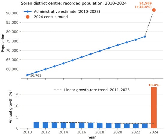
The 2010–2023 population values behave as a deterministic administrative construction rather than as a measured series. Annual growth declines monotonically from 2.701% in 2011 to 1.956% in 2022, recovering slightly to 2.151% in 2023, and a single linear trend in the growth rate accounts for this pattern with an R2 of 0.882 and a residual standard deviation of 0.092 percentage points. Compounding that rule forward from the 2010 base reproduces every 2010–2023 level to within 0.10%. The 2024 observation departs sharply from the same construction: growth of 18.393% against 1.976% expected from the trend, a deviation of 178 residual standard deviations, consistent with the 2024 census round replacing an estimate rather than with a year of demographic change.
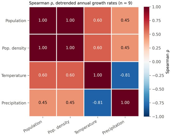
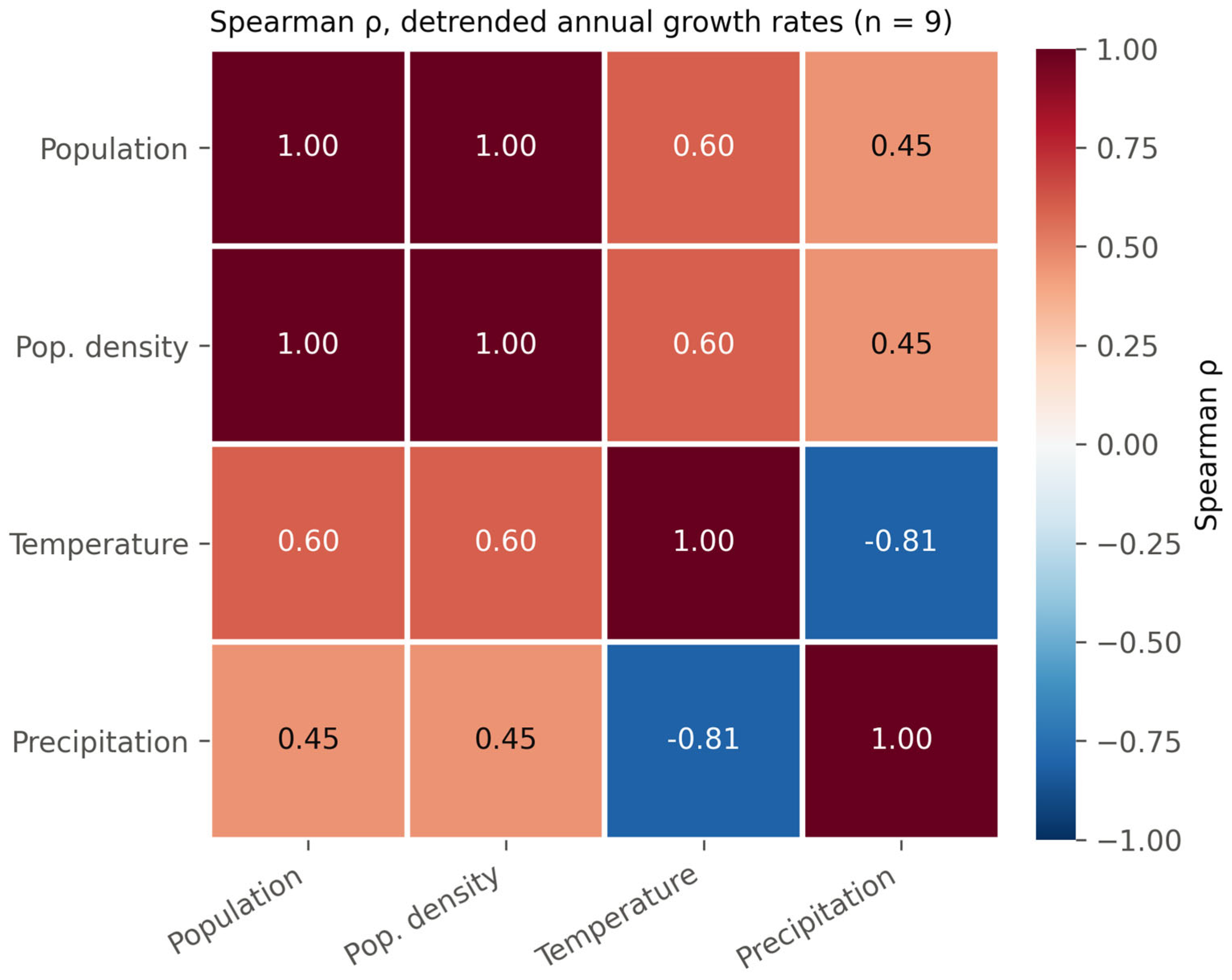
Bivariate correlation analysis (Spearman’s ρ) was computed on the 2015–2024 climate–population overlaps with both series detrended, testing population growth against mean annual temperature, total precipitation, mean relative humidity and total pan evaporation at lags of 0, 1 and 2 years (twelve combinations; n = 9 growth-rate pairs at lags 0 and 1, n = 8 at lag 2). One combination reached nominal significance—humidity at lag 0, ρ = 0.78, p = 0.013—and did not survive correction for multiple testing (Holm–Bonferroni p = 0.150; Benjamini–Hochberg p = 0.150). The contemporaneous temperature and precipitation coefficients were ρ = 0.60 (p = 0.088) and ρ = 0.45 (p = 0.224); every lag-1 and lag-2 coefficient fell between −0.48 and 0.27 with p ≥ 0.23. Because the pre-2024 population values are generated by the smooth rule described above, their year-on-year variation carries no independent demographic signal, and this result is therefore reported as an inability of the available data to resolve a climate–demography association rather than as an absence of one. Temperature and precipitation themselves showed a strong inverse monthly relationship (ρ = −0.806, p < 0.001, n = 120), consistent with the region’s distinct wet and dry seasonal regimes.
Figure 2 Spearman correlation heatmap (Population, Population density, Temperature, and Precipitation) computed on the cleaned data. Population and population density are correlated with climate at lag 0 using annual, detrended, year-over-year growth rates (n = 9 pairs); the temperature–precipitation cell reflects the monthly relationship (n = 120), which describes genuine intra-annual climate structure and carries no small-sample concern. Population and population density are perfectly correlated by construction. Lagged results are reported in Section 3.1 rather than shown here, since a single heatmap can display only one lag at a time. The population rows should be read in light of Section 3.1: the pre-2024 values are administratively smoothed, so they do not measure a demographic response to climate.
Figure 2.
Spearman correlation heatmap.
Because population density is obtained by dividing the same population values by a constant area of 2135 km2, its correlation with population and with all other variables is mathematically identical to population’s by construction and provides no additional information; it is retained in the heatmap only for interpretability in per-km2 units. Density rose from 26.6 persons per km2 in 2010 to 42.9 in 2024.
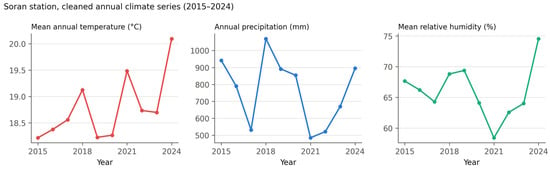
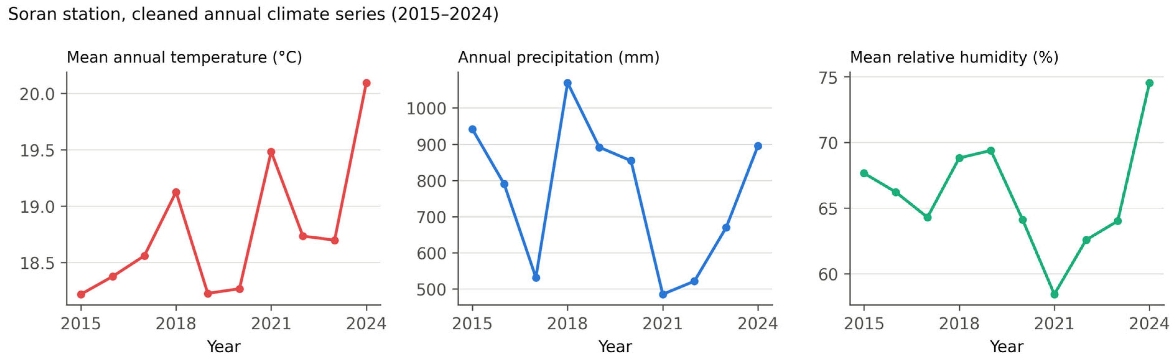
Figure 3 shows the cleaned annual climate aggregates for 2015–2024: mean annual temperature, annual precipitation total, and mean relative humidity. It replaces the scatter of monthly climate values against a spline-interpolated monthly population series shown in the previous version, which could not support inference about population because the population values plotted were interpolation output rather than observations. Mean annual temperature ranges from 18.06 °C (2023) to 20.09 °C (2024), and annual precipitation ranges from 485 mm (2021) to 1070 mm (2018), with a mean of 765 mm. The formal test of the climate–population relationship is the annual, detrended, lagged correlation reported in Section 3.1.
Figure 3.
Cleaned annual climate series, Soran station, 2015–2024.
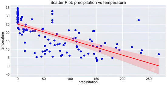
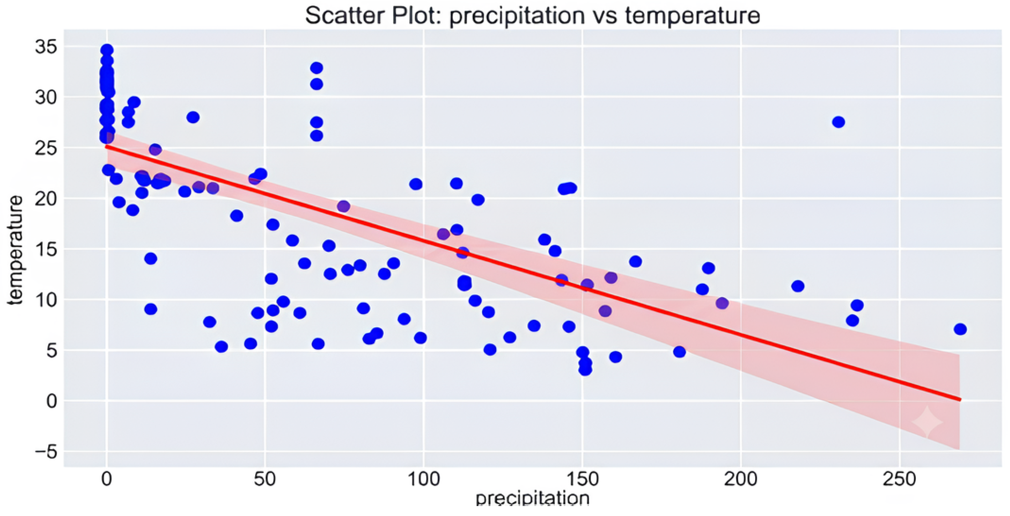
The analysis revealed a strong and statistically significant negative monotonic association between air temperature and precipitation in the cleaned monthly record (Spearman’s ρ = −0.806, p < 0.001, n = 120). As shown in Figure 4, precipitation events are concentrated during periods of lower temperature, while the highest temperatures coincide with near-zero precipitation; the fitted trend line is shown for visual illustration of this pattern. This reflects the study area’s pronounced seasonal cycle: cooler, wetter conditions predominate outside the summer months, while warmer, drier conditions predominate during summer, consistent with a Mediterranean or semi-arid continental climate.
Figure 4.
Correlation between precipitation and temperature. Blue points represent individual monthly observations, the red line shows the fitted linear regression, and the shaded band represents its 95% confidence interval.
3.2. Predictive Performance and Cross-Model Comparison
The Vector Autoregression results reported in the previous version have been withdrawn together with the specification itself (Section 2.5.1) because they characterized the circularity of population-derived predictors rather than any property of the population series and cannot be recomputed on the corrected data without reintroducing those predictors.
Under rolling-origin cross-validation (Section 2.9), the results differ qualitatively from those reported in the previous version, and they are most informative when the seven folds are split at the census year. Across all seven folds, a random walk with drift attains the lowest MAPE (2.05%), and with a linear trend (2.09%), the large MLP (2.15%) and the second-order polynomial (2.17%) close behind, while the AIC-selected ARIMA (4.19%) is no better than a naïve carry-forward (4.04%). Restricting attention to the six inter-censal folds, every trend-following specification becomes extremely accurate, and the ranking is unchanged: drift 0.087%, linear trend 0.167%, large MLP 0.211%, polynomial 0.227%. These figures are not evidence of forecasting skill. They follow directly from the input series being generated by a smooth growth rule (Section 3.1): a one-parameter drift model with nothing to fit reproduces it more accurately than any fitted alternative. On the seventh fold—the census year—every specification errs by at least 11,663 persons, because a rebasing is not a forecastable quantity.
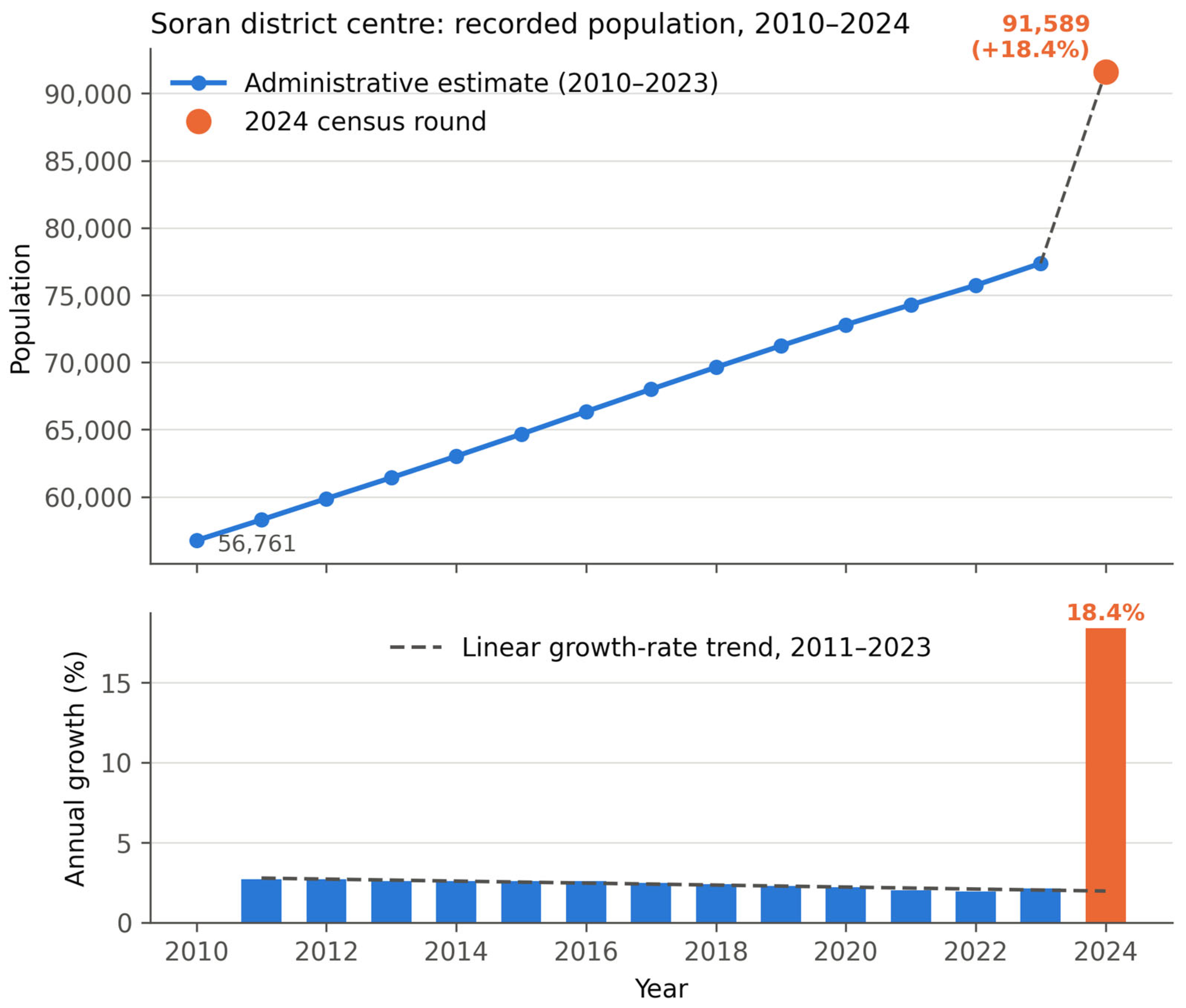
Figure 5 shows the recorded population series and its annual growth rates. The upper panel distinguishes the 2010–2023 administrative estimates from the 2024 census observation; the lower panel plots annual growth together with the linear growth rate trend fitted to 2011–2023. The 2010–2023 segment lies almost exactly on that trend, which is the visual form of the 0.10% reproduction error reported in Section 3.1, while the 2024 bar stands at 18.4% against a fitted 1.98%. This figure replaces the population-versus-smoothed-precipitation panel of the previous version, which plotted a spline-interpolated monthly population series.
Figure 5.
Recorded population and annual growth rate, Soran district center, 2010–2024.
3.3. Statistical Significance of Forecast Accuracy
Pairwise Diebold–Mariano tests were applied to the rolling-origin forecast errors of all six fitted specifications, in both the seven-fold and the six-fold samples (Section 2.9). Across all seven folds, none of the fifteen pairwise comparisons reaches significance at the 5% level: the census-year error dominates the loss differential for every model and swamps the differences between them. On the six inter-censal folds, eight of the fifteen comparisons reach nominal significance, with the random walk with drift significantly more accurate than the log-linear trend (DM = −3.00, p = 0.030) and the second-order polynomial (DM = −2.90, p = 0.034), and the small MLP significantly worse than every other specification (Table 3). These results confirm that the drift model tracks a smooth administrative rule most closely; they are not evidence of demographic forecasting skill, and with only six independent errors, they remain suggestive rather than confirmatory (Section 4.3).
Table 3.
Diebold–Mariano test results (rolling-origin, squared-error loss, Harvey–Leybourne–Newbold small-sample correction). Selected comparisons: the complete set of fifteen pairwise tests for both samples is provided in the reproducibility package. A negative DM statistic indicates that Model 1 carries the smaller squared-error loss.
Meteorological Seasonality
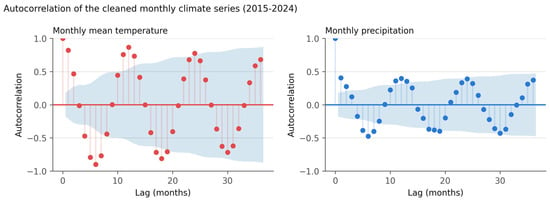
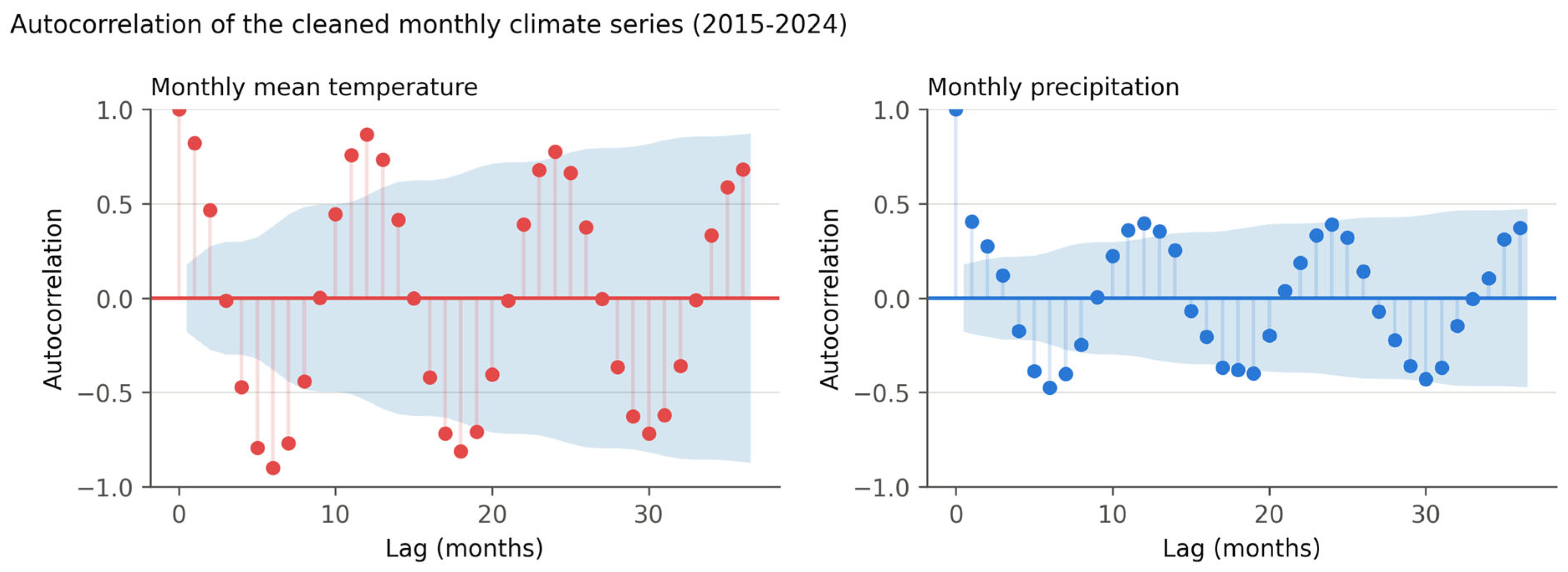
Temperature: the autocorrelation function of the cleaned monthly series shows a clear sinusoidal pattern with a 12-month period (Figure 6), indicating annual seasonality. The Augmented Dickey–Fuller test yields a p-value of 0.4231, so the null hypothesis of a unit root cannot be rejected, and the series is treated as non-stationary; for a strongly seasonal monthly series, this primarily reflects the seasonal cycle itself rather than a stochastic trend.
Figure 6.
Autocorrelation of the cleaned monthly climate series (2015–2024).
Precipitation: the cleaned rainfall series shows a weaker but still clear 12-month signal together with substantial noise (Figure 6). The ADF test produced a p-value of 0.0767, indicating marginal non-stationarity at the 5% significance level. The moving-average smoothing reported in the previous version has been withdrawn: smoothing mechanically reduces high-frequency variance and can lower ADF p-values independently of the underlying process, so the lower p-value obtained from a smoothed series did not establish stationarity and is not reported as a result.
Figure 6 shows the autocorrelation functions of monthly mean temperature and monthly precipitation over 2015–2024, both computed on the cleaned record. Both display the 12-month periodicity expected of a Mediterranean–continental seasonal regime, with temperature the stronger and more regular of the two. No population autocorrelation function is shown: the corresponding panel in the previous version was computed on a spline-interpolated monthly population series and described the interpolation rather than the population, while the annual series has fifteen observations, which is too few to estimate an autocorrelation function. The annual series is nonetheless the sole basis for all population forecasting and validation results reported in this manuscript.
3.4. Vector Autoregression (VAR)—Withdrawn
The VAR results of the previous version are withdrawn (Section 2.5.1 and Section 3.2). No VAR model is fitted to the corrected series, and no VAR forecasts are reported.
3.5. Performance of the ARIMA Specification
On the corrected series, the AIC grid search selects ARIMA(0,2,2) with a 2024 census step term. Under rolling-origin validation, in which the step term is unavailable to the folds preceding it, the specification performs poorly relative to the trend models (MAPE 4.19%, RMSE 5670, R2 0.300 across all seven folds; MAPE 2.64% and R2 −0.750 on the six inter-censal folds), reflecting the difficulty of estimating a second-differenced model on short training windows. Fitted to the full series with the step term, however, it is stable and well behaved: residual diagnostics pass (Ljung–Box p = 0.883; Jarque–Bera p = 0.761), the estimated level shift is 12,564 persons, and the 2025–2030 forecast is monotonic and agrees with the growth-rate projection to within 488 persons in 2030 (Table 2). Its analytic 95% confidence interval, roughly ±500 persons in 2030, is not reported as the study’s uncertainty statement (Section 2.8). No exogenous socio-economic terms are included (Section 2.4), and no causal claim is made regarding the 2024 level shift, whose origin is a change in measurement instrument rather than a demographic event.
3.6. Deterministic Trend Specifications Across the Census Break
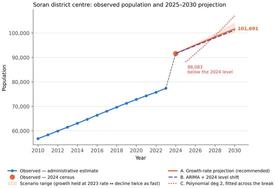
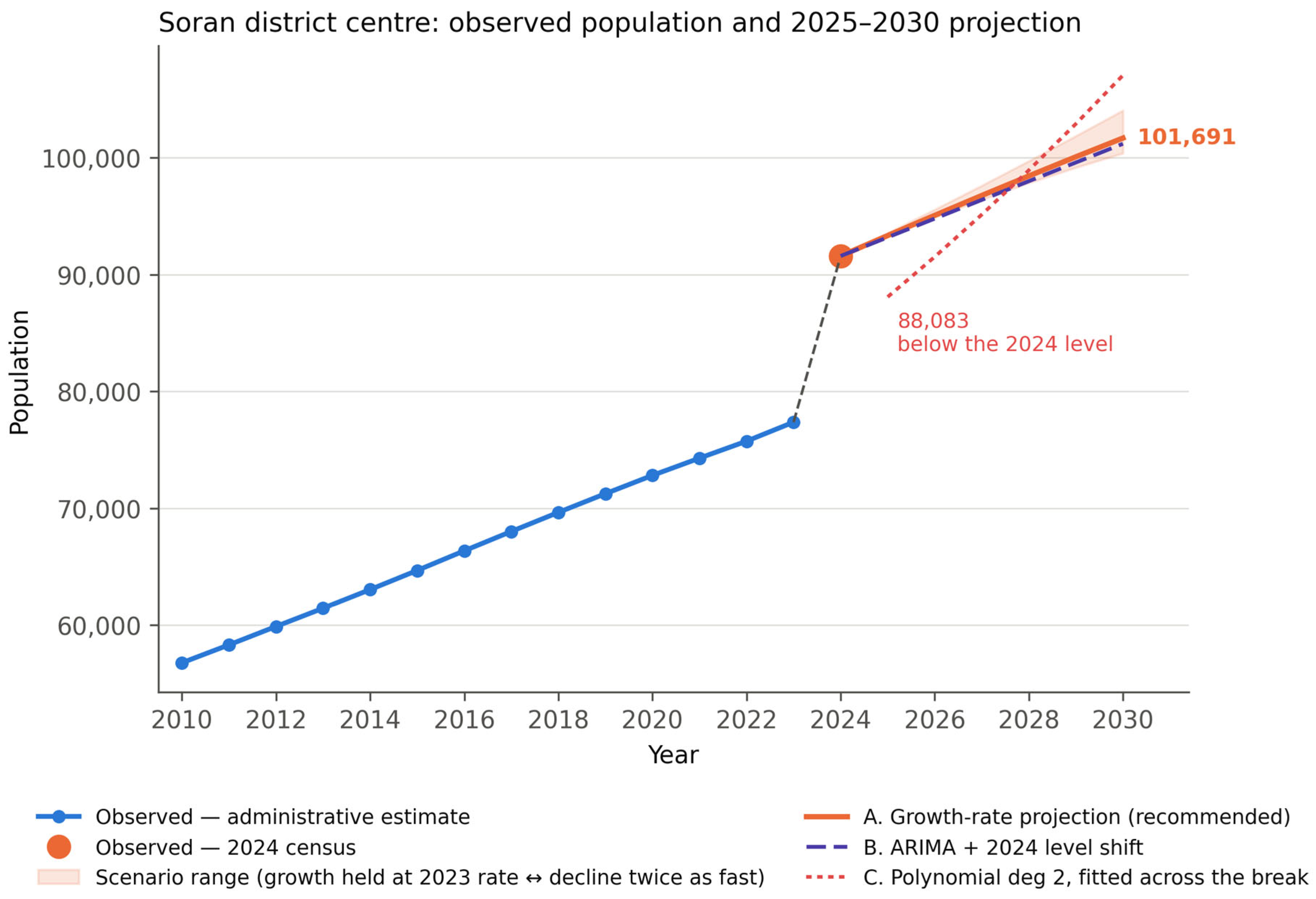
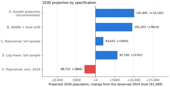
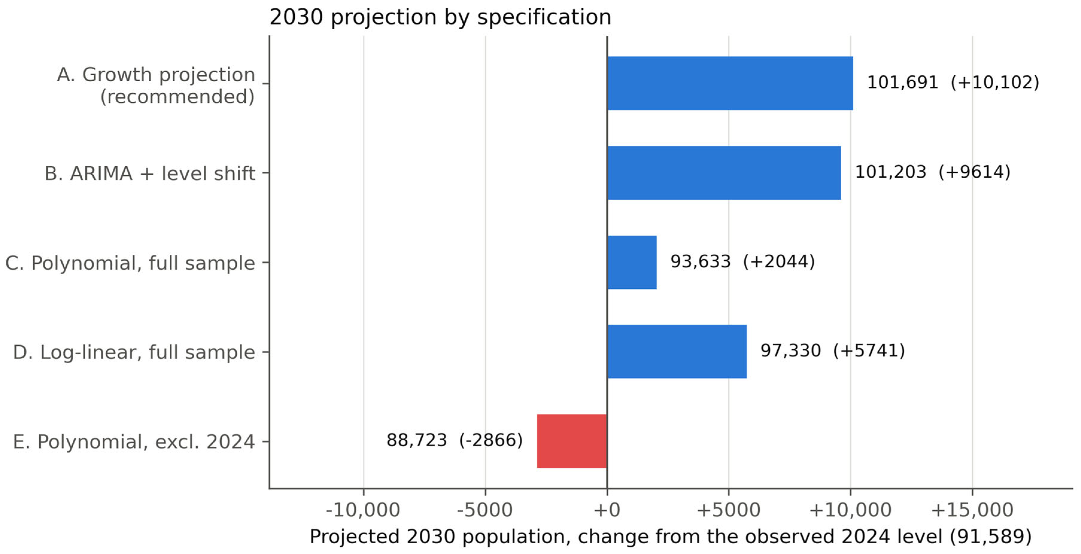
Fitted to the full 2010–2024 series, the second-order polynomial and the log-linear trend both fail in a specific and instructive way. Their 2025 projections are 88,083 and 84,891, respectively—3506 and 6698 persons below the population actually observed in 2024 (Figure 7 and Figure 8). The same polynomial fitted to 2010–2023 alone projects 80,502 for 2025 and 88,151 for 2030, remaining below the 2024 observation throughout the forecast horizon. A smooth trend fitted across a change in measurement instrument averages the two levels, and the resulting projection is an artifact of that averaging rather than a demographic statement. This is the direct answer to the question of whether the second-order polynomial specification retained in the previous version is appropriate for this series: on the corrected data, it is not.
Figure 7.
Soran district center: observed population (2010–2024) and 2025–2030 projection. The recommended growth-rate projection is shown with its scenario range, together with the ARIMA(0,2,2) with a 2024 level shift and the second-order polynomial fitted across the break, which falls below the observed 2024 level in 2025.
Figure 8.
Projected 2030 population by specification, expressed as change from the observed 2024 level (91,589 persons). Specifications that model the census rebasing as a level shift (A, B) agree closely; those fitted across it (C, D, E) diverge, and the polynomial fitted to 2010–2023 alone (E) projects a 2030 population below the 2024 observation.
The reported projection indicates continued growth from 91,589 in 2024 to 101,691 in 2030, an increase of 11.0% over six years at annual rates declining from 1.91% to 1.60% (Table 2). Both the point trajectory and the scenario range should be read as indicative. The range spans the growth-rate assumption only; it does not include uncertainty in the 2024 census level itself, and a revision of that base figure would move all six projected years proportionally. A second post-census observation is required before the post-2024 growth rate can be estimated from data rather than assumed (Section 4.3).
3.7. In-Sample Fit of the Polynomial Model
Fit to the full 2010–2024 annual series, the second-order polynomial model achieved an in-sample coefficient of determination (R2) of 0.925, a Mean Absolute Percentage Error of 2.14%, and a Root Mean Square Error of 2388. Fitted to the 2010–2023 segment alone, it achieved an in-sample R2 of 0.9998 and a MAPE of 0.09%. The contrast between these two figures is itself a finding: the near-perfect fit on the inter-censal segment measures agreement with an administrative interpolation rule, and the drop once the census year is included measures the size of the level shift. Neither statistic is evidence of forecasting skill, which is addressed by the out-of-sample results in Table 4, Table 5 and Table 6.
Table 4.
Rolling-origin out-of-sample performance across all seven folds (test years 2018–2024). Rows are ordered by MAPE.
Table 5.
Rolling-origin out-of-sample performance across the six inter-censal folds (test years 2018–2023), with scale-free measures. Rows are ordered by MASE. Every fitted specification is outperformed by the random walk with drift on this segment.
Table 6.
Fold-level absolute forecast errors (persons) by test year under rolling-origin validation. The 2024 column tests the census rebasing rather than a year of demographic change, and no specification is within an order of magnitude of its own inter-censal errors there. Model labels are abbreviated; full specifications are given in Table 4 and Table 5.
3.8. The Growth Equation
Two fitted equations are reported. Equation (3) is the growth-rate trend that generates the recommended projection, estimated on the observed annual growth rates for 2011–2023. Equation (4) is the second-order polynomial in levels, fitted to the sample 2010–2024. In both, t = year − 2010.
g(t) = 2.845 − 0.0620 t (g in per cent per year; R2 = 0.882)
P(t) = 58,091 + 652 t + 89.9 t2 (in-sample, 2010–2024; R2 = 0.925)
Interpretation of Coefficients:
In Equation (3), the intercept (2.845%) is the fitted growth rate in 2010, and the slope (−0.0620 percentage points per year) is the rate at which annual growth has been declining; extrapolating this trend produces the assumed rates in Table 2. Equation (4) is reported for completeness: its positive quadratic term (+89.9 t2) indicates convexity, but that convexity is produced by the 2024 census rebasing rather than by accelerating demographic growth, and the specification’s projections are reported as a failure case (Section 3.6) rather than as the study’s forecast.
3.9. Rolling-Origin Out-of-Sample Performance Summary
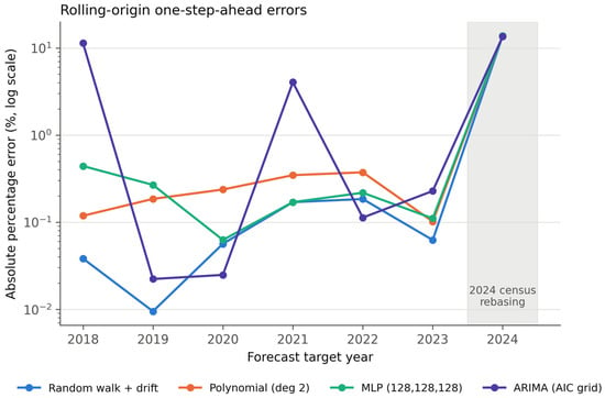
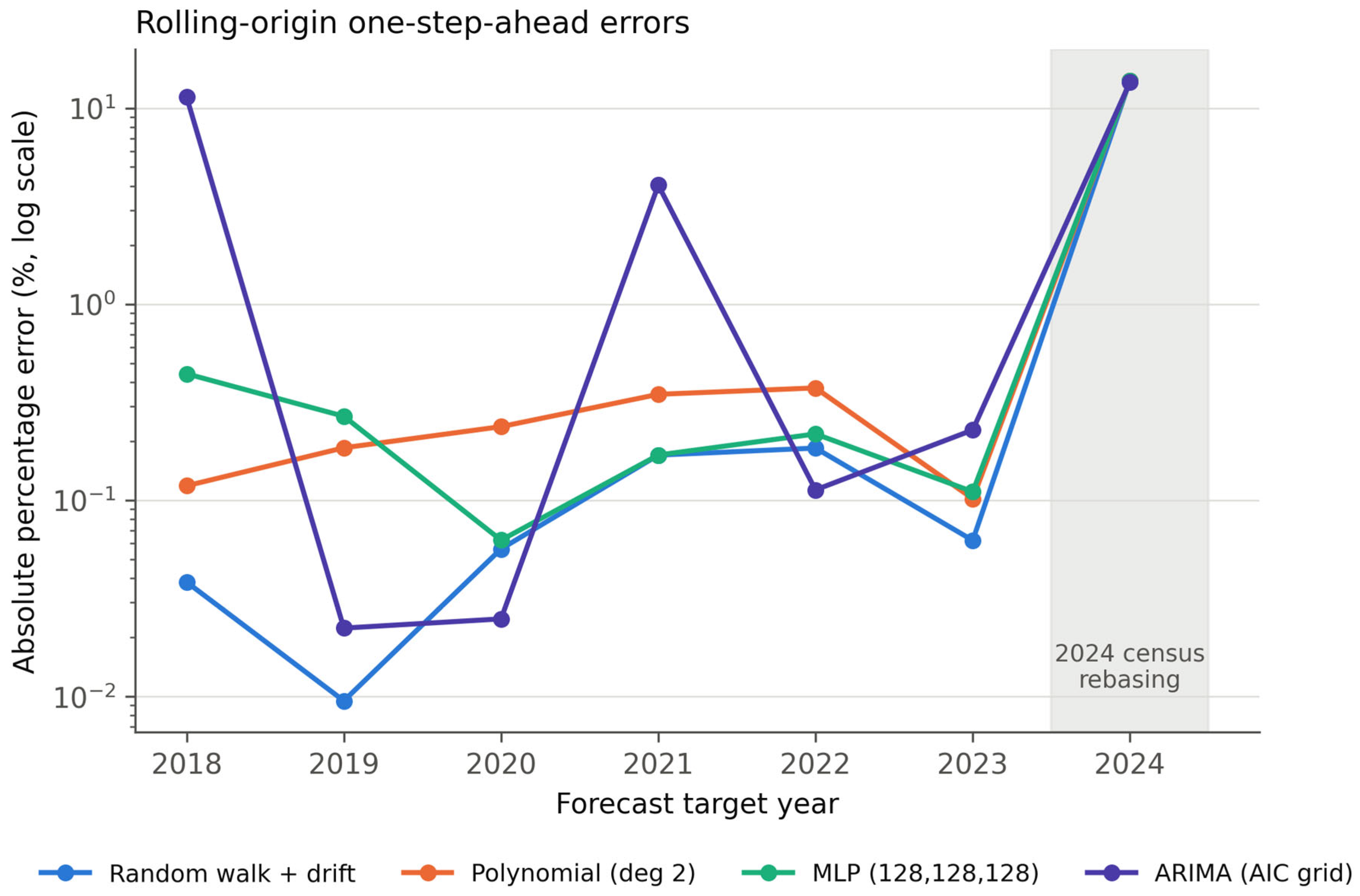
Table 4 and Table 5 report the rolling-origin out-of-sample performance of all eight specifications, first across all seven folds (test years 2018–2024) and then across the six inter-censal folds alone. Table 6 gives the fold-level absolute errors, which are the most informative view of these results. Two patterns dominate. First, on the inter-censal folds every trend-following specification is accurate to a fraction of a percent, and the most accurate is the random walk with drift (MAPE 0.087%, MASE 0.041)—a one-parameter model with nothing to fit. Second, on the 2024, fold every specification errs by between 11,663 and 17,424 persons (Figure 9). The aggregate statistics across all seven folds are dominated by that single fold, which is why they are reported in two panels rather than one.
Figure 9.
Rolling-origin one-step-ahead absolute percentage errors by test year and specification (logarithmic scale). The shaded band marks the 2024 census-rebasing fold, on which every specification fails by two orders of magnitude more than on the inter-censal folds.
To establish whether the fitted specifications improve on trend-following alternatives, three deliberately simple benchmarks—a naïve last-observation forecast, a random-walk-with-drift model, and a simple OLS linear trend—were evaluated under the identical rolling-origin protocol (train 2010–(2009 + k), forecast one step ahead, k = 8,…,14), with all parameters refitted within each fold. Two scale-free measures accompany the absolute ones: the Mean Absolute Scaled Error (MASE), in which each fold’s absolute error is divided by the mean one-step naïve absolute error inside that fold’s own training window, and the ratio of each model’s mean absolute error to that of the naïve benchmark on the same targets (RelMAE). Values below 1 indicate an improvement on the corresponding benchmark.
Three features of this comparison should be emphasized. First, no fitted specification improves on the random walk with drift on the inter-censal folds; the second-order polynomial, which was the retained model in the previous version, is 2.6 times less accurate than drift by MAPE and 2.6 times less accurate on the naïve-relative scale. Second, all of these very low errors belong to a segment of the data generated by an arithmetic rule, so they quantify the smoothness of the input rather than the skill of the model, and none should be reported as forecast accuracy. Third, the comparison is dominated by a single fold: every specification misses the 2024 census year by between 11,663 and 17,424 persons, whereas the six inter-censal folds produce errors of at most a few thousand and typically a few hundred. Performance statistics computed from seven forecast targets, one of which tests a change in measurement instrument, should therefore be regarded as unstable, and the benchmark comparison as a whole argues against reporting any of these models as demonstrating demographic forecasting skill on this series.
4. Discussion
The primary empirical finding of this study concerns the data as much as the phenomenon. Across twelve variable–lag combinations, no association between annual population growth and local hydro-climatic variability survived correction for multiple testing (Section 3.1). This is reported neither as evidence that population dynamics are independent of climate nor as a detected absence of association, but as a limit of what the available series can resolve: the 2010–2023 population values are inter-censal estimates produced by a smooth administrative rule, so their year-on-year variation is not a demographic measurement that could respond to climate, and the single post-census observation cannot supply one. Establishing whether climate and demography are coupled in Soran requires a population series measured independently in each year, which does not currently exist for the district.
The forecasting results are consistent with recent findings in the small-area population forecasting literature. In a comprehensive review of small-area demographic forecasting methods, Wilson et al. [26] report that studies applying machine learning to short, sparse demographic series have generally found traditional statistical and extrapolative methods to be more accurate and computationally efficient than machine learning alternatives and note that claims of machine learning superiority in this literature often stem from inadequate baseline comparisons. This echoes the broader time-series forecasting literature: Makridakis, Spiliotis, and Assimakopoulos [27] found that machine learning methods, including neural network architectures, were consistently less accurate than classical statistical benchmarks across thousands of real-world series, with the performance gap widening as series length decreased. Our finding that neither multilayer perceptron improved on a random walk with drift—and that no fitted trend specification did either—is therefore consistent with that pattern rather than an anomaly specific to Soran: with fifteen annual observations, this dataset falls squarely within the regime where data-intensive architectures are structurally disadvantaged relative to low-parameter models. The present analysis adds a further consideration. Where the target series is itself an administrative interpolation, model comparison measures agreement with the interpolation rule, and any apparent superiority over a naïve benchmark is a statement about the smoothness of the input rather than about forecasting skill. Reporting the provenance of the demographic series is therefore a precondition for interpreting forecast-accuracy statistics in small-area work, not a supplementary detail—a point that generalizes well beyond the Kurdistan Region context examined here.
These findings should be interpreted with caution. Whether socio-economic pull factors are masking environmental constraints on population growth in Soran is a plausible hypothesis worth investigating with genuinely independent socio-economic data (Section 4.2), but it is not demonstrated by the present analysis and could not be, given the provenance of the demographic series. Similarly, continued population growth alongside a variable regional rainfall regime is a planning consideration that may warrant a dedicated water-demand and supply-capacity assessment; the present study does not itself constitute such an assessment and does not quantify water-resource consequences [28].
The inability to detect a short-term association between population growth and the examined hydro-climatic variables should not be interpreted as evidence that environmental conditions are unimportant for demographic change in the district. The broader climate–demography literature indicates that demographic responses to environmental stress are often mediated by economic conditions, migration, infrastructure, institutional capacity, and access to resources rather than occurring as direct responses to climate variability alone. In rapidly growing semi-arid urban areas, population growth can persist despite short-term hydro-climatic variability where migration, employment opportunities, housing development, or urban services provide stronger demographic incentives. Testing that proposition in Soran, however, requires demographic data capable of recording such responses; the 2010–2023 estimates by construction cannot.
4.1. Research Contributions
The contribution of the present study is not to demonstrate climate–demography independence nor to establish a forecasting model for Soran, but to provide a transparent and reproducible demographic baseline for the district together with an explicit account of what its administrative provenance permits. The study also contributes a worked protocol for a situation that is common in data-scarce settings and rarely reported: a short annual series in which part of the record is an administrative interpolation and one observation is a census rebasing. The diagnostics used here—reproducing the series with a growth-rate rule, splitting rolling-origin results at the break, and benchmarking against a naïve carry-forward—are inexpensive and would identify the same problem in other small-area datasets.
4.2. Future Research
Future research should test this interpretation along four complementary lines. First, and most directly, an independently measured demographic record is needed. The binding constraint here is not only the length of the series but also its construction: extending a series generated by an interpolation rule would not increase the information available for testing a climate–demography relationship. Annual administrative counts, civil-registration totals, or utility-connection records that are measured rather than estimated would be more valuable than additional years of the present series. Where such data are not obtainable in the near term, pooling across structurally similar districts within the Kurdistan Region—following the “borrowing strength” approach used in the small-area population forecasting literature, where forecasts for individual small areas are improved by exploiting patterns learned across a wider collection of comparable series—offers a practical route to increasing effective sample size without waiting for additional years of local observation.
Second, genuinely independent indicators of migration, housing development, employment, and economic activity are needed, distinct from the population-derived proxies excluded from the present analysis. Candidate sources include administrative building-permit and utility-connection records; labor force survey data, where available; and remittance or bank-transfer indicators as proxies for economic activity.
Third, these indicators should be embedded within a multivariate framework capable of distinguishing direct climatic effects from socio-economic mediation and delayed demographic response—for example, a mediation analysis or structural equation modeling framework in which housing and employment variables are explicitly modeled as intermediaries between hydro-climatic variability and population change, rather than treated as parallel, independent predictors as in the present univariate approach.
Fourth, future work should move beyond the stationary-climatology assumption of the present study by incorporating non-stationary climate-change projections (e.g., CMIP6 scenario data) and high-resolution remote-sensing indicators of land-cover change, urban expansion, and water-resource availability, allowing demographic forecasts to be conditioned on plausible future hydro-climatic trajectories rather than an assumption of climatic stationarity.
4.3. Limitations
Three limitations bound the claims made here. First, and most consequentially, the 2010–2023 population values are inter-censal estimates rather than measurements. They are reproduced to within 0.10% by a single declining-growth rule, which means that the out-of-sample accuracy statistics in Table 4 and Table 5 measure agreement with that rule and not demographic forecasting skill and that the climate–demography tests in Section 3.1 are performed against a series with no independent year-to-year variation. No analysis of these data, however carefully validated, can overcome this.
Second, the 2024 observation is not comparable with those preceding it. It derives from the 2024 census round and represents a level shift of 12,564 persons rather than a year of growth. Because only one post-census observation exists, the post-2024 growth rate cannot be estimated from data and is assumed from the pre-census trend; the projection in Table 2 is conditional on that assumption, and its scenario range does not include uncertainty in the census base itself. A second post-census observation would allow the assumption to be tested directly.
Third, the rolling-origin scheme yields only seven out-of-sample test points, six of which lie on the administratively smoothed segment. All comparative model-performance claims, including the Diebold–Mariano results, should therefore be interpreted as suggestive rather than confirmatory. The study also includes no independently observed socio-economic predictors (local GDP, housing completions, migration, or employment records) and is framed as an exploratory univariate trend extrapolation of population; the reported forecasts should not be read as evidence that socio-economic factors contribute to population growth in Soran.
5. Conclusions
This research examined the relationship between climatic variability and demographic dynamics in the Soran district center using a comparative multi-model framework applied to the official 2010–2024 annual population series and the 2015–2024 monthly meteorological record. Four points follow from the revised analysis.
First, no association between population growth and temperature, precipitation, humidity or evaporation survived correction for multiple testing across twelve variable–lag combinations. Because the 2010–2023 population values are administratively smoothed inter-censal estimates, this is reported as a limit of what the available data can resolve, not as evidence of climate–demography decoupling; such a conclusion would require an independently measured annual series and explicit analysis of non-stationarity, migration responses, and indirect water-availability pathways.
Second, the provenance of the demographic series determines what the forecasting results mean. A single linear growth-rate rule reproduces the 2010–2023 levels to within 0.10%, and under rolling-origin validation a random walk with drift forecasts that segment to a mean absolute percentage error of 0.087%—more accurately than the second-order polynomial, the ARIMA, or either neural network. These accuracies describe the input series rather than the models and are reported as such rather than as evidence of forecasting skill.
Third, the 2024 census round introduces a level shift of 12,564 persons that no specification anticipates; every model errs by at least 11,663 persons on that fold. Deterministic trends fitted across the break project 2025 populations are below the observed 2024 value and are reported as specification failures. The projection retained anchors on the census level instead and extrapolates the 2011–2023 growth-rate trend, giving 101,691 residents by 2030 within a scenario range of 100,395 to 104,064, corroborated to within 488 persons by an ARIMA(0,2,2) with a census step term.
Fourth, the socio-economic proxies used in the original submission were direct mathematical transformations of population and remain excluded, as does the Vector Autoregression specification that depended on them. The study is framed as an exploratory univariate trend-extrapolation exercise, and no causal or predictive claims are made regarding socio-economic drivers of population growth. Its contribution lies in establishing a transparent and reproducible demographic baseline for a rapidly urbanizing, data-scarce district, together with an explicit account of the data and methodological limitations that bound its current claims. Future research should prioritize an independently measured annual population series, a second post-census observation, and genuine socio-economic indicators (employment, housing completions, and migration records), alongside the integration of non-stationary climate-change projections (e.g., CMIP6 scenarios) and high-resolution remote-sensing data, to assess more rigorously the long-term intersection of demographic expansion, climate variability, and groundwater availability.
Supplementary Materials
The following supporting information can be downloaded at: https://www.mdpi.com/article/10.3390/geographies6030094/s1. Table S1. MLP architecture sensitivity analysis: regularization settings and rolling-origin out-of-sample performance on the six inter-censal folds (test years 2018–2023). The random walk with drift is shown for reference. The single-linear-unit architecture reported in the previous version has been dropped, since the 8 × 8 network already establishes that reducing capacity does not rescue the approach. Table S2. Climate quality-assurance log, summarized by rule (120 station-months, 2015–2024). The complete cell-level log, including every original value and its replacement, is provided in the reproducibility data.
Author Contributions
Conceptualization, S.R.H. and K.J.A.; Formal analysis, S.R.H., A.R. and K.J.A.; Investigation, A.R.; Methodology, S.R.H., A.R. and K.J.A.; Software, S.R.H. and K.J.A.; Validation, S.R.H. and K.J.A.; Visualization, S.R.H.; Writing—original draft, S.R.H. and K.J.A.; Writing—review and editing, A.A.M. and A.R. All authors have read and agreed to the published version of the manuscript.
Funding
This research received no external funding.
Institutional Review Board Statement
Not applicable.
Informed Consent Statement
Not applicable.
Data Availability Statement
All data, analysis code, required Python packages (3.12), and generated outputs used in this study are openly available in a GitHub repository to facilitate reproducibility: https://github.com/Azad77/soran-population-forecast (accessed on 6 September 2026). The revised analysis reported here is contained in the reproducibility package Soran_Population_Forecast_Clean.ipynb, which reads the two raw input workbooks and regenerates every table and figure in this manuscript, together with a run manifest recording the random seed (42), package versions, and SHA-256 checksums of the input files.
Conflicts of Interest
The authors declare no conflicts of interest.
References
- Trask, B.S. Migration, Urbanization, and the Family Dimension. Background paper prepared for the United Nations Department of Economic and Social Affairs, Division for Inclusive Social Development, Focal Point on the Family. 2022. Available online: https://www.un.org/development/desa/family/wp-content/uploads/sites/23/2022/04/Migration-Urbanization-and-the-Family-Dimension-by-Bahira-Trask.pdf (accessed on 6 September 2026).
- Liang, W.; Zhang, W.; Jin, Z.; Yan, J.; Lü, Y.; Li, S.; Yu, Q. Rapid Urbanization and Agricultural Intensification Increase Regional Evaporative Water Consumption of the Loess Plateau. J. Geophys. Res. Atmos. 2020, 125, e2020JD033380. [Google Scholar] [CrossRef] [Scilit]
- El Kenawy, A.M. Hydroclimatic Extremes in Arid and Semi-Arid Regions: Status, Challenges, and Future Outlook. In Hydroclimatic Extremes in the Middle East and North Africa; Elsevier: Amsterdam, The Netherlands, 2024; pp. 1–22. [Google Scholar]
- Jónsson, G. The Environmental Factor in Migration Dynamics-a Review of African Case Studies; International Migration Institute: Oxford, UK, 2010. [Google Scholar]
- Xu, D.; Wang, Y.; He, K.; Li, H.; Dong, Y.; Kuang, J.; Zhang, Z.; Song, B.; Niu, Y.; Sun, G. A 500-Year Cycle of Demographic Expansion and Contraction in the Lower Yangtze and Adjacent Coastal Region during the Holocene Driven by East Asian Summer Monsoon Oscillations. Quat. Sci. Rev. 2026, 376, 109815. [Google Scholar] [CrossRef] [Scilit]
- Jończy, R.; Śleszyński, P.; Dolińska, A.; Ptak, M.; Rokitowska-Malcher, J.; Rokita-Poskart, D. Environmental and Economic Factors of Migration from Urban to Rural Areas: Evidence from Poland. Energies 2021, 14, 8467. [Google Scholar] [CrossRef] [Scilit]
- Kibonde, S.F. Socio-Economic Impacts of Internal Migration Dynamics in Morogoro Municipality, Tanzania. Tanzan. J. Popul. Stud. Dev. 2024, 31, 35–54. [Google Scholar] [CrossRef] [Scilit]
- Flörke, M.; Schneider, C.; McDonald, R.I. Water Competition between Cities and Agriculture Driven by Climate Change and Urban Growth. Nat. Sustain. 2018, 1, 51–58. [Google Scholar] [CrossRef] [Scilit]
- He, C.; Liu, Z.; Wu, J.; Pan, X.; Fang, Z.; Li, J.; Bryan, B.A. Future Global Urban Water Scarcity and Potential Solutions. Nat. Commun. 2021, 12, 4667. [Google Scholar] [CrossRef] [Scilit]
- Muttarak, R. Demographic Perspectives in Research on Global Environmental Change. Popul. Stud. 2021, 75, 77–104. [Google Scholar] [CrossRef] [Scilit]
- Wisner, B.; Pelling, M.; Mascarenhas, A.; Holloway, A.; Ndong, B.; Faye, P.; Ribot, J.; Simon, D. Small Cities and Towns in Africa: Insights into Adaptation Challenges and Potentials. In Urban Vulnerability and Climate Change in Africa; Pauleit, S., Coly, A., Fohlmeister, S., Gasparini, P., Jørgensen, G., Kabisch, S., Kombe, W.J., Lindley, S., Simonis, I., Yeshitela, K., Eds.; Future City; Springer International Publishing: Cham, Switzerland, 2015; Volume 4, pp. 153–196. [Google Scholar]
- Sumari, N.S.; Cobbinah, P.B. Secondary Cities in African Urbanization: On Urban Expansion and Density Patterns in Tanzania’s Mid-Sized Cities. Appl. Geogr. 2026, 186, 103859. [Google Scholar] [CrossRef] [Scilit]
- Hamad, R. A Remote Sensing and GIS-Based Analysis of Urban Sprawl in Soran District, Iraqi Kurdistan. SN Appl. Sci. 2020, 2, 24. [Google Scholar] [CrossRef] [Scilit]
- OĞUZ, H.; Hassan, T.K.; Omar, F.O. The Spatial Analysis of the Terrain Impact on Agricultural Land Use by Using GIS and RS Techniques: A Case Study of Soran District-Erbil-Iraq. Zanco J. Hum. Sci. 2020, 24, 269–289. [Google Scholar] [CrossRef] [Scilit]
- Agudelo-Vera, C.M.; Mels, A.R.; Keesman, K.J.; Rijnaarts, H.H. Resource Management as a Key Factor for Sustainable Urban Planning. J. Environ. Manag. 2011, 92, 2295–2303. [Google Scholar] [CrossRef] [Scilit]
- Huruta, A.D. Predicting the Unemployment Rate Using Autoregressive Integrated Moving Average. Cogent Bus. Manag. 2024, 11, 2293305. [Google Scholar] [CrossRef] [Scilit]
- Ciommi, M.; Egidi, G.; Salvia, R.; Cividino, S.; Rontos, K.; Salvati, L. Population Dynamics and Agglomeration Factors: A Non-Linear Threshold Estimation of Density Effects. Sustainability 2020, 12, 2257. [Google Scholar] [CrossRef] [Scilit]
- Yao, X.; Qu, Y.; Zhang, L.; Mishra, A.K.; Yin, J.; Ding, R.; Yang, J.; Bai, C.; Zhang, L.; Li, M. Socio-Demographic Factors Shape Mortality Risk Linked to Compound Drought-Heatwave Events under Climate Change in China. One Earth 2024, 7, 2034–2048. [Google Scholar] [CrossRef] [Scilit]
- Xu, K.; Zhang, M.; Li, J.; Du, S.S.; Kawarabayashi, K.; Jegelka, S. How Neural Networks Extrapolate: From Feedforward to Graph Neural Networks. In Proceedings of the 9th International Conference on Learning Representations (ICLR), Virtual Event, Austria, 3–7 May 2021. [Google Scholar]
- Kakraool, M.I.; Hameed, H.M. Rainwater Harvesting as a Sustainable Solution for Managing Water Resources in the Soran Region-Case Study. EURASIAN J. Sci. Eng. 2025, 11, 168–198. [Google Scholar] [CrossRef] [Scilit]
- Diebold, F.X.; Mariano, R.S. Comparing Predictive Accuracy. J. Bus. Econ. Stat. 1995, 13, 253–263. [Google Scholar] [CrossRef] [Scilit]
- Harvey, D.; Leybourne, S.; Newbold, P. Testing the Equality of Prediction Mean Squared Errors. Int. J. Forecast. 1997, 13, 281–291. [Google Scholar] [CrossRef] [Scilit]
- Hyndman, R.J.; Koehler, A.B. Another Look at Measures of Forecast Accuracy. Int. J. Forecast. 2006, 22, 679–688. [Google Scholar] [CrossRef] [Scilit]
- Holm, S. A Simple Sequentially Rejective Multiple Test Procedure. Scand. J. Stat. 1979, 6, 65–70. [Google Scholar]
- Benjamini, Y.; Hochberg, Y. Controlling the False Discovery Rate: A Practical and Powerful Approach to Multiple Testing. J. R. Stat. Soc. Ser. B 1995, 57, 289–300. [Google Scholar] [CrossRef] [Scilit]
- Wilson, T.; Grossman, I.; Alexander, M.; Rees, P.; Temple, J. Methods for Small Area Population Forecasts: State-of-the-Art and Research Needs. Popul. Res. Policy Rev. 2022, 41, 865–898. [Google Scholar] [CrossRef] [Scilit]
- Makridakis, S.; Spiliotis, E.; Assimakopoulos, V. Statistical and Machine Learning Forecasting Methods: Concerns and Ways Forward. PLoS ONE 2018, 13, e0194889. [Google Scholar] [CrossRef] [Scilit]
- Scanlon, B.R.; Fakhreddine, S.; Rateb, A.; De Graaf, I.; Famiglietti, J.; Gleeson, T.; Grafton, R.Q.; Jobbagy, E.; Kebede, S.; Kolusu, S.R. Global Water Resources and the Role of Groundwater in a Resilient Water Future. Nat. Rev. Earth Environ. 2023, 4, 87–101. [Google Scholar] [CrossRef] [Scilit]

Disclaimer/Publisher’s Note: The statements, opinions and data contained in all publications are solely those of the individual author(s) and contributor(s) and not of MDPI and/or the editor(s). MDPI and/or the editor(s) disclaim responsibility for any injury to people or property resulting from any ideas, methods, instructions or products referred to in the content. |
© 2026 by the authors. Licensee MDPI, Basel, Switzerland. This article is an open access article distributed under the terms and conditions of the Creative Commons Attribution (CC BY) license.