


Abstract
Non-grain production of cultivated land has increasingly affected regional food security and the stability of agricultural ecosystems. In traditional rice-producing regions, changes associated with non-rice cultivation, fallow land, rice-fishery integrated farming, and intensive agricultural management are reshaping the spatial structure of paddy landscapes. To identify the long-term spatiotemporal evolution of paddy systems, this study investigated Northern Jiangxi, China, using Landsat surface reflectance imagery from 2000, 2005, 2010, 2015, and 2020 on the Google Earth Engine (GEE) platform. The Enhanced Vegetation Index (EVI) and Land Surface Water Index (LSWI) were used to construct a phenology-based Flooding Frequency (FF) indicator. Based on the annual frequency with which pixels satisfied the condition LSWI > EVI, cultivated land was classified into three categories: non-flooded cropland, standard rice paddy, and high-frequency flooded cropland. In this study, non-flooded cropland was used as an indicator of potential non-rice cultivation rather than as direct evidence of confirmed non-grain production. Landscape metrics, transition matrices, gravity center migration, standard deviation ellipses, and geographically weighted regression (GWR) were then used to examine paddy landscape dynamics, fragmentation patterns, and county-level spatial associations with socioeconomic factors. The results suggest that the paddy system in Northern Jiangxi experienced marked stage-based fluctuations between 2000 and 2020. Standard rice paddy recovered during 2005–2010, whereas non-flooded cropland expanded considerably during 2010–2015, accompanied by intensified paddy landscape fragmentation. Non-flooded cropland was mainly distributed around urban fringes, transport corridors, and some hilly margins. Standard rice paddy was concentrated in traditional grain-producing areas, including the Poyang Lake Plain and the Gan-Fu Plain. High-frequency flooded cropland was primarily located in low-lying lake areas, where its dynamics were likely associated with rice-fishery integrated farming, continuous irrigation, and hydrological fluctuations. Landscape metrics showed that the largest patch index and mean patch size of standard rice paddy declined after 2010, indicating reduced spatial continuity of core paddy fields. The GWR analysis provided auxiliary evidence that total population, per capita gross domestic product (GDP), and urbanization rate were spatially associated with changes in non-flooded cropland at the county level; however, the results should be interpreted as exploratory associations rather than causal mechanisms. Overall, paddy landscape change in Northern Jiangxi was expressed not only through changes in cultivated land area, but also through the reorganization of paddy function, spatial continuity, and land-use intensity. Future cropland protection should therefore move beyond area-based control toward integrated management of quantity, quality, function, and spatial configuration. Future research should further verify these findings using dynamic cropland boundaries, higher-resolution imagery, and more detailed socioeconomic data.
1. Introduction
Food security remains a central concern in land-use management and agricultural policy, particularly in China, where the population is large and per capita cultivated land resources are relatively limited. Traditional cropland protection research has often focused on cultivated land area, requisition–compensation balance, and the effects of urban expansion on cropland quantity. In recent years, however, a more subtle but equally important transformation has emerged within cultivated land itself [1]. Driven by changes in agricultural profitability, rising labor costs, market demand, and urban–rural spatial restructuring, some cropland formerly used for grain production has gradually shifted toward orchards, nursery stock, vegetables, facility agriculture, rice-fishery integrated farming, or fallow and abandoned land. These processes are commonly described as non-grain production of cultivated land. Existing studies have shown that non-grain production is not only a national-scale food-security issue, but also a spatially differentiated land-use process influenced by urbanization, market demand, terrain conditions, and local agricultural management contexts [2,3,4,5,6,7,8,9,10].
Non-grain production does not merely involve a change in crop type. It also modifies the spatial structure of agricultural landscapes. Traditional paddy fields usually have high spatial continuity and stable irrigation systems, making them essential components of food production and agricultural ecosystems in southern China. When continuous paddy fields are divided into different management types and land-use forms, formerly contiguous paddy patches may be fragmented into smaller landscape units. Consequently, mechanized farming efficiency may decline, irrigation and drainage systems may become less integrated, and ecological connectivity within agricultural landscapes may be weakened. Identifying the landscape pattern of paddy fields under non-grain production is therefore important for understanding food security risks and agricultural ecosystem stability [11,12].
Long-term remote sensing monitoring in southern rice-growing regions is challenging. Conventional land-use data and statistical yearbooks provide useful information on cultivated land area and agricultural production, but their spatial resolution is often insufficient to capture internal structural changes within paddy systems. At the same time, cloudy and rainy conditions in southern China often affect single-date remote sensing images, while phenological differences may further complicate classification. Previous research has shown that rice fields exhibit a distinctive flooding signal during the transplanting period. When the land surface is flooded, the Land Surface Water Index (LSWI) often exceeds the Enhanced Vegetation Index (EVI). Consequently, phenology-based approaches using the relationship between LSWI and EVI can be used to extract rice paddy areas, particularly in long-term time-series analyses [13,14,15]. Studies conducted in the Poyang Lake Plain further demonstrate that multi-source and phenology-based rice mapping is especially useful in cloudy and fragmented landscapes of southern China [15].
Nevertheless, three gaps remain. First, although non-grain production has been analyzed at national, regional, coastal, and hilly-area scales, relatively few studies have focused on how non-grain production reorganizes the internal structure of traditional paddy landscapes in southern rice-producing plains [7,8,9,10]. Second, many remote-sensing studies have focused primarily on rice planting area, while paying less attention to paddy landscape fragmentation, patch connectivity, and spatial configuration, despite the established value of landscape metrics for assessing fragmentation and structural change [16,17,18,19]. Third, the factors associated with non-grain production are spatially heterogeneous. In peri-urban areas, non-grain production may be related to land opportunity costs and market demand, whereas in remote mountainous or traditional agricultural areas, it may be associated with rural labor outflow, rising agricultural costs, and topographic constraints. A global regression model alone may therefore obscure regional differences; GWR has been widely used to explore spatial non-stationarity in land-use and socioeconomic relationships [20,21,22].
Northern Jiangxi, located on the southern bank of the middle and lower reaches of the Yangtze River, is an important component of the Poyang Lake Ecological Economic Zone and a major grain-producing region in Jiangxi Province. The area contains traditional rice-producing zones such as the Poyang Lake Plain and the Gan-Fu Plain, while also being affected by the expansion of Nanchang, Jiujiang, Jingdezhen, and other urban centers. These conditions make Northern Jiangxi a representative region for investigating paddy landscape change and potential non-grain production risk. In this study, we used Landsat time-series imagery from 2000 to 2020 to construct a cropland utilization classification based on EVI, LSWI, and annual FF. We then combined landscape metrics, transition matrices, gravity center migration, standard deviation ellipses, and GWR to analyze paddy landscape evolution and spatially heterogeneous associations under non-grain production.
The objectives of this study were fourfold: (1) to reconstruct the spatiotemporal distribution of cropland utilization systems in Northern Jiangxi from 2000 to 2020 based on rice phenology; (2) to analyze transitions among non-flooded cropland, standard rice paddy, and high-frequency flooded cropland; (3) to reveal paddy landscape fragmentation and spatial migration patterns; and (4) to explore county-level spatial heterogeneity between changes in non-flooded cropland and population scale, economic development, and urbanization.
2. Study Area and Data Sources
2.1. Study Area
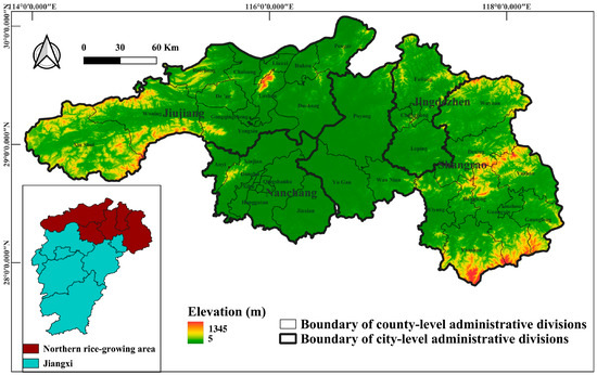
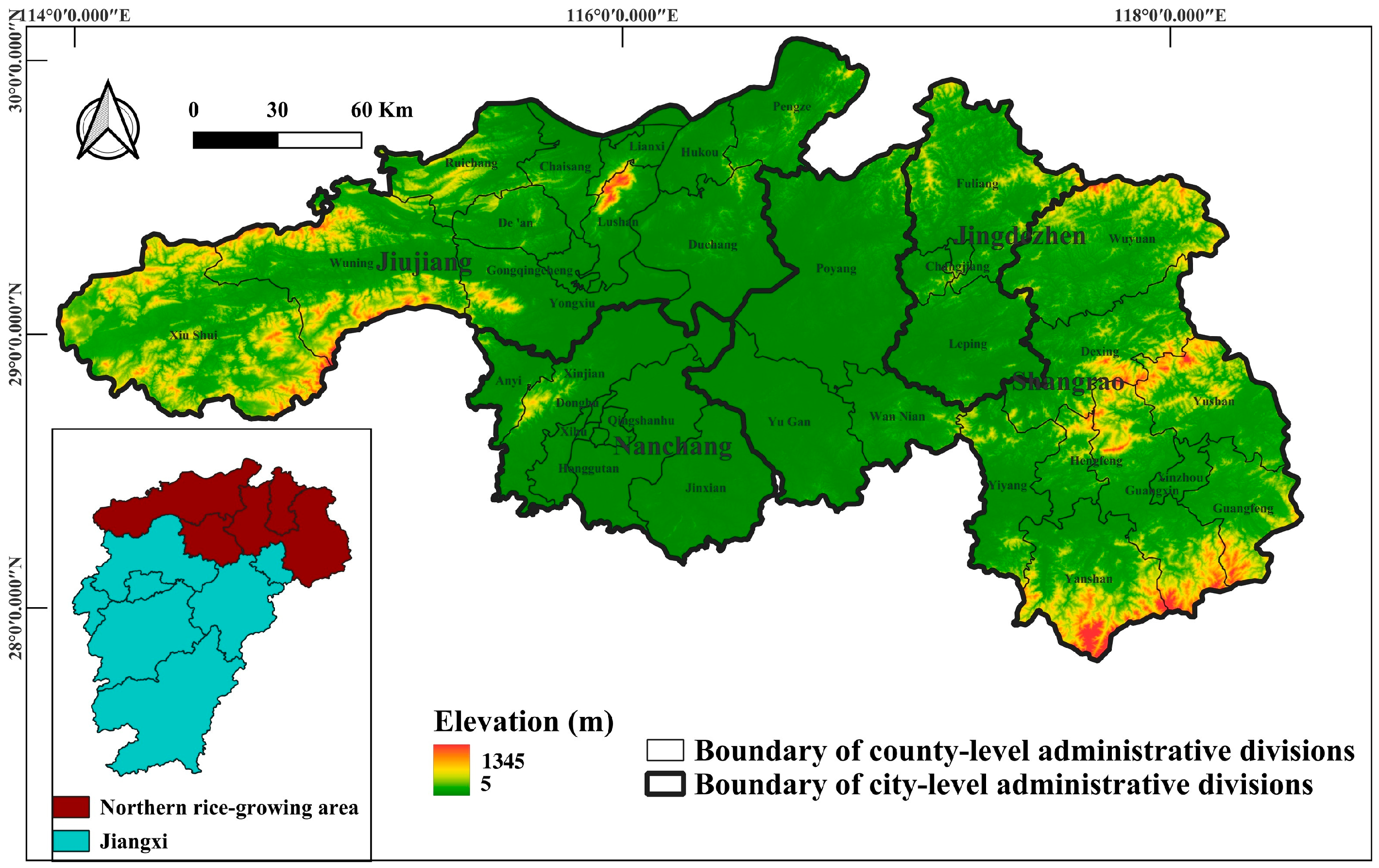
The location and administrative boundary of the study area are shown in Figure 1.
Figure 1.
Location and administrative boundary of the study area in Northern Jiangxi, China.
Northern Jiangxi is located on the southern bank of the middle and lower reaches of the Yangtze River. It is a region where economic development, food production, and ecological conservation are closely intertwined. The study area includes Nanchang, Jiujiang, Jingdezhen, and surrounding counties, and lies within the core area of the Poyang Lake Ecological Economic Zone. Topographically, the area transitions from surrounding hilly and mountainous terrain to central lacustrine plains and river valleys. The Poyang Lake Plain and the Gan-Fu Plain constitute major contiguous cropland and rice-producing areas.
The study area has a humid subtropical monsoon climate. Mean annual temperature is approximately 16–18 °C, and annual precipitation is approximately 1300–1700 mm. These favorable hydrothermal conditions support single-season rice, double-season rice, and rice-fishery integrated farming. Historically, the region has been an important commodity grain base and traditional rice-producing area in Jiangxi Province.
At the same time, Northern Jiangxi has experienced rapid urbanization and industrial development. With the expansion of the Nanchang metropolitan area, improved transport infrastructure, and rural labor transfer, some traditional paddy fields have gradually shifted toward vegetables, orchards, nursery stock, facility agriculture, and rice-fishery integrated farming. Peri-urban areas are strongly affected by land opportunity costs and market demand, whereas lake areas and hilly regions are jointly influenced by hydrological conditions, topography, and labor restructuring. The region is therefore suitable for examining paddy landscape change, potential non-grain production risk, and spatially heterogeneous mechanisms.
2.2. Data Sources
A dataset covering five observation years—2000, 2005, 2010, 2015, and 2020—was constructed. It included remote sensing imagery, cropland masks, topographic data, socioeconomic data, and validation data.
First, remote sensing imagery was obtained from Landsat surface reflectance products on Google Earth Engine (GEE; Google LLC, Mountain View, CA, USA; https://earthengine.google.com/, accessed on 25 July 2026). Landsat 5 TM and Landsat 7 ETM+ images were mainly used for 2000, 2005, and 2010, whereas Landsat 8 OLI images were mainly used for 2015 and 2020. All images were surface reflectance products suitable for vegetation and water index calculations [23].
Second, cropland extent was derived from the GlobeLand30 global land cover dataset provided by the National Geomatics Center of China (NGCC). The original analysis used the 2010 GlobeLand30 cropland class as a fixed baseline mask to ensure spatial consistency among years and to focus on internal land-use structure changes within existing cropland. This treatment is consistent with the use of GlobeLand30 for large-scale cropland monitoring and fragmentation assessment, although previous research has also shown that cropland area and fragmentation estimates are sensitive to mask selection and temporal coverage [16,24]. To evaluate the influence of the fixed-mask setting on the temporal interpretation, a multi-year cropland union mask was also constructed as a robustness check. This union mask was derived from the 2000, 2010, and 2020 GlobeLand30 cropland layers and represents the maximum potential cropland extent during the study period.
The pixel counts and corresponding areas of the 2000, 2010, 2020, and multi-year union cropland masks are summarized in Supplementary Table S1. Compared with the 2010 fixed mask, the union mask increased the cropland extent by approximately 2234.66 km2, or 12.71%. This comparison suggests that using only the 2010 mask may exclude areas that existed as cropland in 2000 or 2020. Accordingly, the main analysis is interpreted as an investigation of internal land-use structure changes within the 2010 baseline cropland extent, rather than as a complete accounting of all cropland gains and losses during 2000–2020. The potential limitation of mask selection is further discussed in the limitations section.
Third, topographic data were obtained from the SRTM 30 m Digital Elevation Model. Slope was extracted to describe the topographic context and potential natural constraints on cropland utilization.
Fourth, socioeconomic data were obtained from the Jiangxi Statistical Yearbook, including county-level total population, per capita GDP, and urbanization rate. Because these variables were available at the administrative-unit scale, the GWR analysis was conducted at the county level. The potential Modifiable Areal Unit Problem (MAUP) and ecological fallacy are explicitly discussed below.
Fifth, validation information was mainly obtained from historical high-resolution imagery in Google Earth Pro (Google LLC, Mountain View, CA, USA; https://www.google.com/earth/versions/, accessed on 25 July 2026). For early years with limited high-resolution imagery or temporal mismatch, visual interpretation was supported by Landsat false-color composite imagery, topographic context, stable land-cover features, and paddy texture characteristics. The validation information was used to support the reliability assessment of the classification results rather than to claim a fully independent pixel-level quantitative accuracy assessment.
3. Methods
The methodological workflow consisted of five main steps. First, Landsat time-series imagery was acquired and preprocessed on GEE. Second, EVI and LSWI were calculated, and annual FF was derived. Third, cropland utilization systems were classified according to FF values. Fourth, transition matrices, the expansion intensity index, landscape metrics, gravity center migration, and standard deviation ellipses were used to analyze paddy landscape evolution. Fifth, county-level population, economic development, and urbanization variables were incorporated into a GWR model to explore spatially heterogeneous associations with changes in non-flooded cropland. The overall methodological workflow is summarized in Supplementary Figure S1. Spatial analyses, including gravity-center migration, SDE, and GWR, were conducted in ArcGIS 10.8 (Esri, Redlands, CA, USA).
3.1. Remote Sensing Image Acquisition and Preprocessing
To capture cropland utilization changes under different policy and market backgrounds, 2000, 2005, 2010, 2015, and 2020 were selected as key observation years. For each year, Landsat images during the rice growing season were obtained, with particular attention to spectral characteristics during the transplanting and growing periods. Image preprocessing was conducted in GEE and included cloud and cloud-shadow masking, radiometric consistency processing, sensor-specific band matching, and study-area clipping.
Clouds, cloud shadows, and other low-quality pixels were removed using bitwise operations on the QA_PIXEL band from Landsat Collection 2 Surface Reflectance products. Because southern China is frequently affected by cloud and rainfall, multi-temporal valid observations were used to reduce the effect of missing pixels in single images on annual FF statistics. To further examine the influence of image availability on annual FF calculation, valid Landsat observations were summarized for each observation year. The number of available images ranged from 89 to 171, and the mean valid observations per pixel ranged from 5.93 to 12.35. The corresponding statistics are provided in Supplementary Table S3. Landsat 7 ETM+ images after 2003 are affected by SLC-off gaps. In this study, multi-temporal valid observations within the same year were used to reduce the influence of such gaps, although residual uncertainty may remain in years dominated by Landsat 7 imagery. The potential effect of Landsat 7 SLC-off gaps is therefore acknowledged in the discussion and limitations sections.
Because Landsat sensors differ slightly in band names and spectral responses, red, near-infrared, blue, and shortwave infrared bands were extracted separately for each sensor to calculate EVI and LSWI. All data were harmonized to a 30 m spatial resolution. Resampling was used to maintain spatial consistency among datasets, but it cannot eliminate mixed-pixel uncertainty at 30 m resolution. Therefore, mixed pixels in fragmented peri-urban cropland and lake–shore transition zones were treated as an important source of uncertainty.
The main analysis used the 2010 GlobeLand30 cropland layer as a fixed baseline mask to ensure spatial consistency across the 2000–2020 time series and to focus on internal land-use structure changes within the baseline cropland extent. To assess the influence of this fixed-mask choice on the core conclusions, a multi-year cropland union mask based on the 2000, 2010, and 2020 GlobeLand30 cropland layers was further constructed as a robustness check. This comparison is important because cropland fragmentation studies based on GlobeLand30 have emphasized that boundary definition and classification consistency can influence area and patch-structure estimates [16,24].
3.2. EVI–LSWI–FF-Based Classification of Cropland Utilization Systems
The rice transplanting period is usually accompanied by artificial flooding, which strengthens the surface water signal. During this stage, LSWI often exceeds EVI; therefore, the condition LSWI > EVI was used as an indicator of rice-field flooding signals. This rule has been widely used in phenology-based paddy rice mapping because it captures the temporary coexistence of surface water and young rice canopy during transplanting and early growth stages [13,14,15]. EVI and LSWI were calculated for each valid Landsat observation as follows:
where , , and represent the near-infrared, red, and blue surface reflectance bands, respectively [25].
where represents the shortwave infrared surface reflectance band.
For each observation year, every valid observation of each pixel was evaluated against the condition LSWI > EVI. If the condition was met, the pixel was assigned a value of 1, indicating a flooding signal at that observation time. Otherwise, it was assigned a value of 0. The annual FF of each pixel was then calculated by summing all valid observations satisfying this condition:
where denotes the annual flooding frequency, represents a valid Landsat observation within a given year, is the total number of valid observations, and is an indicator function. If , then ; otherwise, .
Because FF counted the number of valid observations satisfying the LSWI > EVI condition within a year, it was interpreted as an annual flooding-signal frequency rather than an exact irrigation frequency. FF = 0 indicates that no clear flooding signal was detected during the available valid observations and was classified as non-flooded cropland. FF = 1–2 was used to represent standard rice paddy because conventional single- or double-season rice systems usually show one or two main flooding signals during the transplanting or early growth period. FF ≥ 3 was interpreted as high-frequency flooded cropland, which may reflect repeated flooding signals associated with intensive paddy management, rice-fishery integrated farming, continuous irrigation, or lake-area hydrological fluctuations. Based on annual FF values, cropland utilization systems were classified into three types, as shown in Table 1.
Table 1.
Classification rules for cropland utilization systems based on annual Flooding Frequency (FF).
Type 1 should not be equated directly with strict non-grain production. Because Landsat imagery and the FF indicator cannot further distinguish dry cropping, orchards, nursery stock, fallow land, abandoned cropland, and other non-rice uses, Type 1 was conservatively defined as non-flooded cropland or a potential non-rice cultivated status. Therefore, the term “non-grain production” in this study refers to a landscape-level risk signal inferred from the conversion of standard rice paddy to non-flooded cropland, rather than a direct crop-type classification result.
3.3. Reliability Assessment
To provide an auxiliary assessment of classification reliability, the classification results for different years were visually examined using Google Earth Pro historical high-resolution imagery, Landsat false-color composite images, and topographic background information [26,27]. For each observation year, representative sample areas were selected for the three cropland utilization types, and their spectral characteristics, spatial textures, and temporal consistency with adjacent years were jointly interpreted.
The validation samples were selected using a stratified visual interpretation strategy. For each observation year, representative samples were selected from the three cropland utilization types and distributed across different spatial contexts, including the Poyang Lake Plain, the Gan-Fu Plain, peri-urban areas, hilly margins, and lake–shore transition zones. The interpretation protocol considered three types of evidence: flooding status derived from Landsat false-color composites and LSWI–EVI behavior, field texture and parcel regularity from Google Earth historical imagery, and temporal consistency with adjacent-year land-cover patterns. This procedure was designed to evaluate whether the classified pixels were spatially and temporally plausible, rather than to produce a fully independent pixel-level accuracy assessment.
Standard rice paddy was mainly identified based on flooding signals during the transplanting or growing season, regular field textures, and relatively stable cultivation patterns. Non-flooded cropland was interpreted based on the absence of obvious flooding signals, vegetation cover characteristics, and changes in land-use patterns. High-frequency flooded cropland was further examined by considering its repeated flooding signals and its spatial association with lake areas, drainage networks, or low-lying terrain. The visual interpretation focused on whether the classified pixels showed reasonable flooding status, field texture, and temporal consistency, rather than on identifying detailed crop species.
Because the spatial and temporal coverage of Google Earth historical high-resolution imagery was limited for 2000 and 2005, fully consistent reference imagery was not available for all early-year samples. Therefore, the validation procedure was used primarily to support the spatial plausibility and long-term temporal interpretation of the classification results, rather than to claim a fully independent pixel-level quantitative accuracy assessment. For the early years, Landsat false-color composite images, stable features in adjacent years, topographic background, and paddy-field texture were jointly used to reduce the uncertainty caused by limited reference imagery.
It should be noted that non-flooded cropland may include dry cropping, orchards, nursery stock, fallow land, abandoned cropland, and other non-rice cultivated conditions. Similarly, high-frequency flooded cropland may be influenced by rice-fishery integrated farming, continuous irrigation, and hydrological fluctuations around lake areas. Therefore, the reliability assessment was mainly used to support the interpretation of flooding status and functional changes in paddy systems, rather than to produce a precise crop-type classification map. In interpreting the results, we avoided presenting the classification as error-free and treated limited early-year reference imagery and within-class heterogeneity as important sources of uncertainty.
3.4. Expansion Intensity Index and Transition Matrix
The Expansion Intensity Index () was used to quantify the expansion or contraction intensity of non-flooded cropland across adjacent periods. EII measures the change in Type 1 area relative to total county-level cropland area and the time interval:
where is the expansion intensity index, and represent the area of Type 1 non-flooded cropland at the beginning and end of the study period, respectively, is the total cropland area within the county, and is the time interval in years.
A transition matrix was also constructed to analyze conversions among Type 1, Type 2, and Type 3. The conversion from Type 1 to Type 2 indicates a shift from non-flooded cropland to standard rice paddy and can be interpreted as rice paddy recovery or re-graining. The conversion from Type 2 to Type 1 indicates a shift from standard rice paddy to non-flooded cropland and may indicate a potential departure from conventional rice cultivation, rather than confirmed non-grain production at the crop-type level. The conversion from Type 2 to Type 3 indicates a shift from standard rice paddy to high-frequency flooded cropland, which may be associated with rice-fishery integrated farming or continuous irrigation. The conversion from Type 3 to Type 1 indicates a shift from high-frequency flooded cropland to non-flooded cropland. To avoid conceptual confusion, this transition was not described as wetland loss.
3.5. Landscape Metrics
Landscape metrics were calculated using FRAGSTATS 4.2 (University of Massachusetts, Amherst, MA, USA) to examine paddy landscape fragmentation. Four metrics were selected: Patch Density (PD), Largest Patch Index (LPI), Aggregation Index (AI), and Mean Patch Size (MPS) [17,18,19,28]. These metrics are commonly used because they jointly describe patch subdivision, core-patch dominance, spatial aggregation, and average patch scale, which are directly relevant to the fragmentation and mechanization potential of paddy landscapes. In this study, PD was expressed as the number of patches per 100 ha, LPI and AI were expressed as percentages (%), and MPS was expressed in hectares (ha). Landscape metrics were calculated in FRAGSTATS using the same neighborhood rule and edge-treatment settings for all observation years to ensure temporal comparability. The analysis was conducted at the class level within the 2010 fixed cropland mask, and areas outside the cropland mask were treated as background and excluded from class-level metric interpretation.
PD represents the number of patches per unit area; higher values indicate greater landscape fragmentation. LPI measures the proportion of the largest patch of a class relative to the total landscape area; higher values indicate stronger dominance of core patches. AI reflects the degree of aggregation among cells of the same class; higher values indicate stronger spatial connectivity. MPS represents average patch area; lower values often imply smaller and more fragmented patches.
The unit of depends on the area unit used in FRAGSTATS.
where is the largest patch index of class i, is the area of patch belonging to class , and is the total landscape area.
where is the mean patch size of class , is the area of patch in class , and is the number of patches of class .
where is the aggregation index of class , is the number of like adjacencies between pixels of class , and is the maximum possible number of like adjacencies for class .
When landscape metrics are summarized by administrative units, the results represent county-level landscape pattern changes. County-level analysis was used because counties are important units for cropland protection, policy implementation, and statistical data collection. Nevertheless, administrative boundaries may split patches and affect patch area and patch counts. This limitation is acknowledged in the limitations section, and future research should consider grid-based or multi-scale analyses.
3.6. Gravity Center Migration and Standard Deviation Ellipse
Gravity center migration and Standard Deviation Ellipse (SDE) analysis were used to characterize broad spatial migration patterns of different cropland utilization systems. The gravity center model calculated the weighted mean spatial center of each class in each year. Patch centroids were used as spatial locations, and patch areas were used as weights [29,30].
SDE analysis was used to describe directional distribution, spatial dispersion, and expansion range. The ellipse center represents the mean location of a spatial distribution, the major axis indicates the dominant expansion direction, the minor axis indicates the secondary direction, and the rotation angle represents the main spatial orientation. By comparing ellipse locations, orientations, and ranges across years, spatial migration and aggregation patterns of different cropland utilization systems were identified.
The weighted gravity center of each cropland utilization type was calculated as follows:
where represents the weighted gravity center coordinates of a given cropland utilization type, are the centroid coordinate of patch , is the area weight of patch , and is the total number of patches.
The standard deviation ellipse of each cropland utilization type was calculated as follows:
where and represent the standard distances along the and directions, respectively. They indicate the spatial dispersion of a given cropland utilization type around its weighted gravity center.
3.7. Exploratory GWR Analysis of County-Level Spatial Associations
In this study, GWR was used as an exploratory tool to examine spatially varying associations, rather than as a confirmatory model for identifying causal mechanisms. Geographically Weighted Regression (GWR) was conducted to explore spatially heterogeneous associations between changes in non-flooded cropland and socioeconomic factors. GWR was selected because it allows regression coefficients to vary across space and is therefore suitable for exploratory analysis of spatial non-stationarity in land-use change and socioeconomic processes [20,21,22]. Because the cropland classification data used for the GWR analysis were derived from the 2005–2010 land-use transition results, whereas the socioeconomic explanatory variables were obtained from the 2011 Jiangxi Statistical Yearbook, the GWR results were interpreted as an exploratory analysis of spatial associations between cropland structure change during 2005–2010 and the socioeconomic context of the adjacent period.
The dependent variable was the county-level change intensity or proportional change in non-flooded cropland during 2005–2010. The explanatory variables included county-level total population, per capita GDP, and urbanization rate in 2011. Total population was used to reflect population scale, per capita GDP to represent economic development and land opportunity costs, and urbanization rate to indicate urban–rural development and labor-structure change. Because the socioeconomic variables were derived from county-level statistics, the GWR analysis primarily reflects county-level spatial associations and should not be interpreted as household-level or pixel-level causality.
The GWR model was specified as follows:
where is the dependent variable for county , representing the change intensity or proportional change in Type 1 non-flooded cropland from 2005 to 2010; denotes the spatial coordinates of county ; represents the -th explanatory variable, including total population, per capita GDP, and urbanization rate; is the spatially varying intercept; is the local regression coefficient; and is the random error term.
Before the GWR model was established, Ordinary Least Squares (OLS) regression was conducted as a global reference model, and the Variance Inflation Factor (VIF) was used to evaluate multicollinearity among explanatory variables. The diagnostic results showed that all VIF values were below the commonly used threshold, with a maximum VIF of 3.102. This indicates that severe multicollinearity was not present and that the selected variables were acceptable for regression analysis.
The GWR model was then used to analyze local spatial relationships between socioeconomic variables and changes in non-flooded cropland across counties. By incorporating spatial weights, GWR allows regression coefficients to vary by location, thereby revealing spatial differences in variable associations. The AICc criterion was used to determine the spatial-weight bandwidth, and the optimal bandwidth was 57,876.63. OLS and GWR were compared using R2, adjusted R2, AICc, and Sigma.
The GWR results were used to identify spatial differences in associations between socioeconomic variables and non-flooded cropland change, rather than to establish strict causality. Given the limited sample size and potential MAUP and ecological fallacy associated with county-level analysis, GWR was treated as an exploratory spatial analysis method, and strong causal language was avoided in the interpretation.
4. Results
4.1. Classification Reliability of Cropland Utilization Systems
The visual reliability assessment based on Google Earth Pro historical imagery, Landsat false-color composites, and topographic background information indicated that the phenology-based method using LSWI, EVI, and FF could generally distinguish standard rice paddy from non-flooded cropland. Standard rice paddy was relatively identifiable in remote sensing images because it usually showed clear flooding signals during the transplanting period or growing season, together with regular field textures and stable cultivation patterns.
Nevertheless, classification uncertainty remained for non-flooded cropland and high-frequency flooded cropland. Non-flooded cropland may include dry cropping, orchards, nursery stock, fallow land, abandoned cropland, and other non-rice cultivated conditions, which are difficult to further separate using Landsat time-series imagery alone. High-frequency flooded cropland may also be affected by rice-fishery integrated farming, continuous irrigation, and hydrological fluctuations around lake areas. In particular, for 2000 and 2005, the limited availability of high-resolution historical reference imagery may have introduced additional uncertainty. Consequently, the classification results were used primarily to identify flooding status and functional changes in cropland systems, rather than as a detailed crop-type classification product. Therefore, the reliability assessment supports the use of the classification results for analyzing relative temporal changes and spatial patterns, but it does not imply that the classification should be treated as a fully validated crop-type map.
4.2. Spatiotemporal Distribution of Cropland Utilization Systems
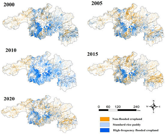
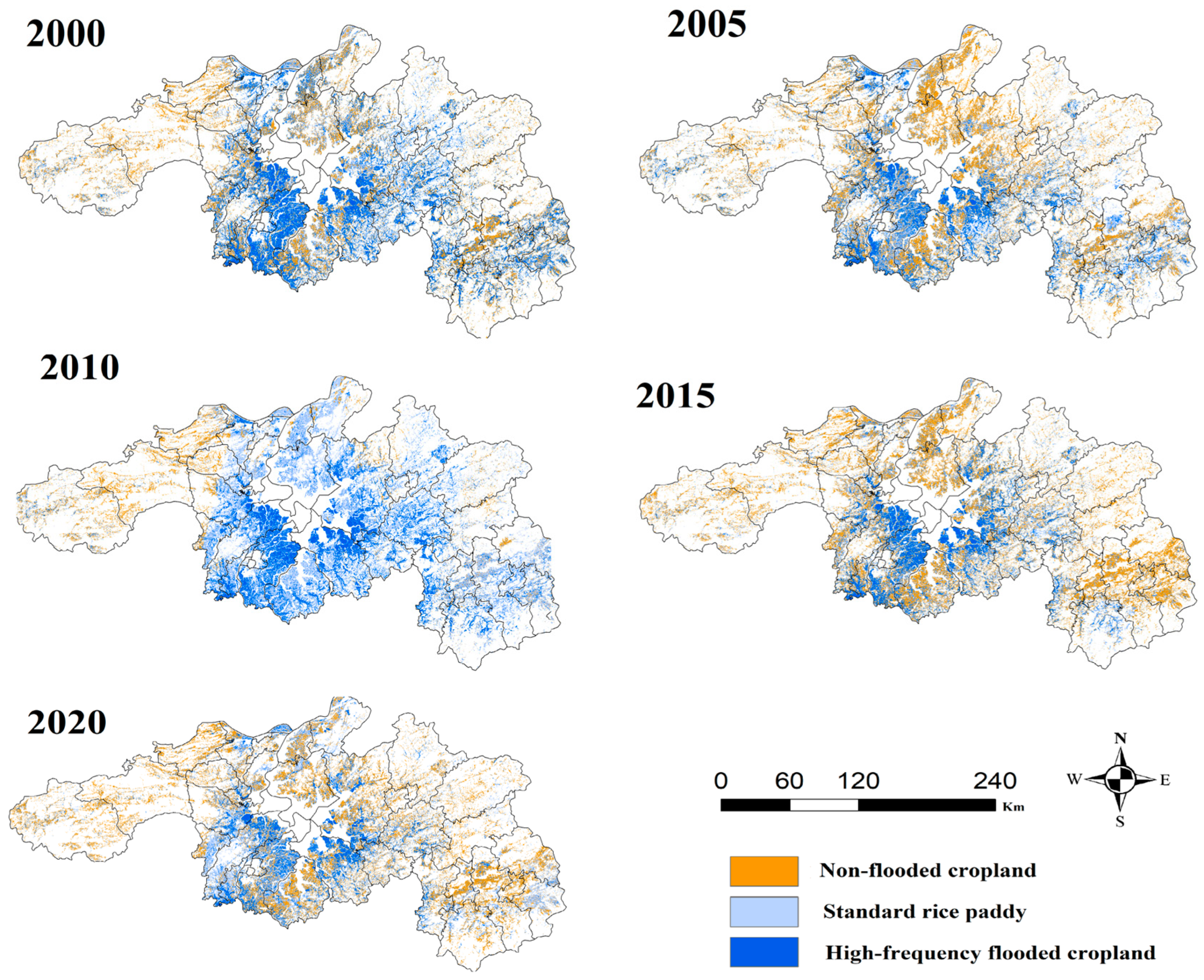
From 2000 to 2020, cropland utilization systems in Northern Jiangxi showed distinct spatial differentiation. Standard rice paddy was mainly distributed in flat areas with favorable hydrothermal conditions, such as the Poyang Lake Plain, the Gan-Fu Plain, and river valleys. These areas constitute the core grain-producing space of the region. Non-flooded cropland was primarily distributed around urban fringes, transport corridors, and some hilly margins. High-frequency flooded cropland was concentrated in low-lying areas and dense water-network zones around Poyang Lake, where its distribution may be related to local hydrological conditions and rice-fishery integrated farming. The spatial distribution of the three cropland utilization systems from 2000 to 2020 is shown in Figure 2.
Figure 2.
Spatial distribution of cropland utilization systems in Northern Jiangxi from 2000 to 2020. Type 1 represents non-flooded cropland, Type 2 represents standard rice paddy, and Type 3 represents high-frequency flooded cropland. The maps show flooding-status-based cropland utilization classes rather than detailed crop-type categories.
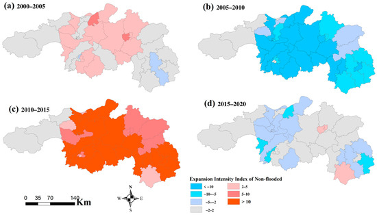
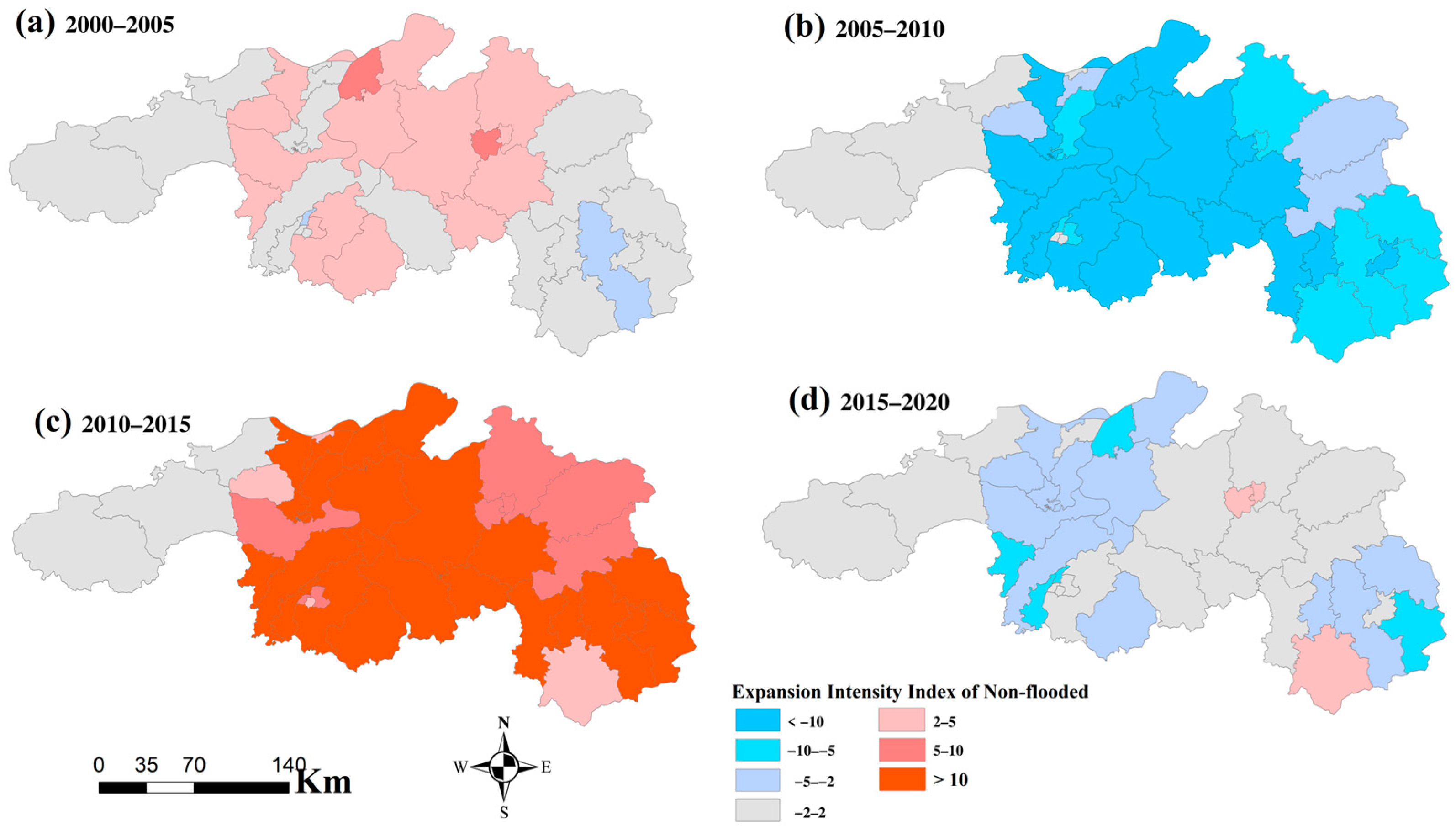
Temporally, standard rice paddy exhibited stage-based fluctuations. During 2000–2005, some standard rice paddy was converted into non-flooded cropland. During 2005–2010, standard rice paddy recovered. During 2010–2015, non-flooded cropland expanded markedly and standard rice paddy decreased substantially. During 2015–2020, standard rice paddy partially recovered, although non-flooded cropland remained spatially evident. The expansion intensity index of non-flooded cropland is shown in Figure 3.
Figure 3.
Spatiotemporal evolution of the expansion intensity index of non-flooded cropland.
4.3. Change Characteristics and Uncertainty Around 2010
The results indicate substantial changes in cropland utilization systems around 2010, especially in the recovery of standard rice paddy and the dynamics of high-frequency flooded cropland. These changes should be interpreted cautiously. On the one hand, the 2005–2010 period may have been influenced by agricultural tax abolition, grain subsidies, and cropland protection policies, which likely enhanced the willingness to maintain rice production. On the other hand, 2010 was also a period in which Landsat 5 and Landsat 7 data were jointly used. In some areas, the results may have been affected by Landsat 7 SLC-off gaps, cloud cover, differences in valid observation counts, and insufficient imagery within specific phenological windows.
Therefore, the changes around 2010 were not attributed to a single policy or market factor. Instead, they were interpreted as a transition period that may reflect the combined influence of cropland-use change and remote sensing observation constraints.
To evaluate whether the use of the 2010 fixed cropland mask influenced the core temporal pattern, the area of Type 2 standard rice paddy was further compared with that derived from the multi-year cropland union mask. The results showed that Type 2 standard rice paddy reached its maximum in 2010 and declined markedly in 2015 under both mask schemes. Although mask selection affected the absolute area estimates of cropland utilization types, it did not alter the main conclusion regarding the stage-based fluctuation of standard rice paddy. The extended comparison of Type 1, Type 2, and Type 3 areas under the two mask schemes is further provided in Supplementary Table S2 and Supplementary Figure S2. This comparison indicates that mask selection affected absolute area estimates, but it did not reverse the main temporal signal of standard rice paddy recovery and decline identified in this study.
4.4. Transition Matrix and Stage-Based Changes
To summarize the dominant transitions among the three cropland utilization systems, the major transition pathways for each period are presented in Table 2.
Table 2.
Main transition pathways among cropland utilization systems from 2000 to 2020.
The transition matrix results show that conversions among cropland utilization systems were stage-dependent. During 2000–2005, the conversion from Type 2 to Type 1 was relatively pronounced, indicating that some standard rice paddy shifted to non-flooded cropland. During 2005–2010, the conversion from Type 1 to Type 2 increased, suggesting rice paddy recovery. During 2010–2015, the conversion from Type 2 to Type 1 increased substantially, indicating accelerated conversion from standard rice paddy to non-flooded cropland. During 2015–2020, the conversion from Type 1 to Type 2 partially recovered, although non-flooded cropland expansion remained evident in peri-urban areas.
The conversion from Type 1 to Type 2 can be interpreted as rice paddy recovery or re-graining, whereas the conversion from Type 2 to Type 1 may indicate a potential departure from conventional rice cultivation, rather than confirmed non-grain production at the crop-type level. The conversion from Type 2 to Type 3 indicates a shift from standard rice paddy to high-frequency flooded cropland, and the conversion from Type 3 to Type 1 represents a shift from high-frequency flooded cropland to non-flooded cropland. To avoid conceptual confusion, the latter was not described as wetland loss.
4.5. Paddy Landscape Fragmentation
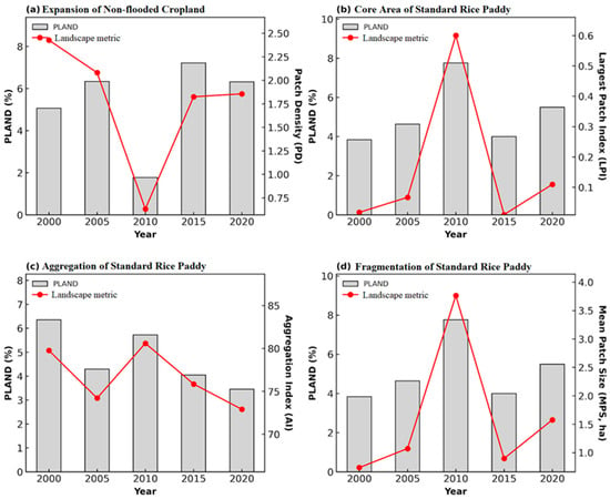
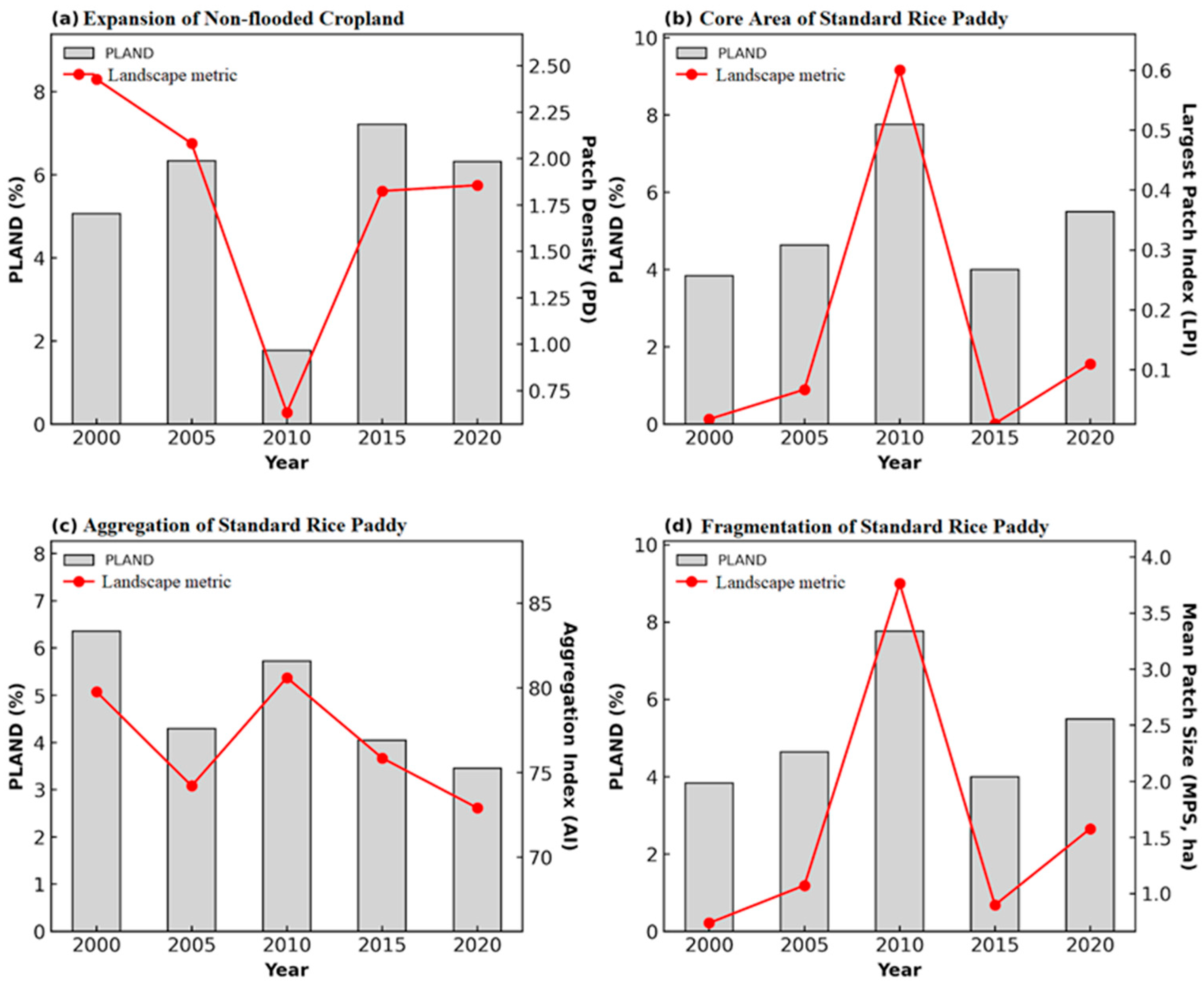
Landscape metrics indicate that paddy landscape change in Northern Jiangxi was not limited to area change, but also involved spatial structural reorganization. The LPI and MPS of standard rice paddy decreased during certain periods, indicating that contiguous paddy patches were split and the spatial integrity of core paddy fields was weakened. The combined increase in PD and decline in MPS suggest intensified fragmentation of standard rice paddy landscapes. Temporal changes in landscape metrics are shown in Figure 4.
Figure 4.
Temporal changes in landscape metrics of cropland utilization systems from 2000 to 2020. The gray bars indicate PLAND (%), and the red lines indicate the corresponding landscape metrics: PD, Patch Density (patches per 100 ha); LPI, Largest Patch Index (%); AI, Aggregation Index (%); and MPS, Mean Patch Size (ha).
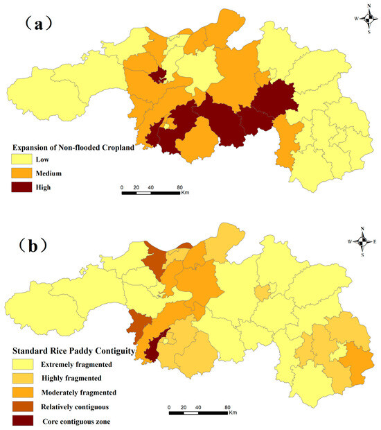
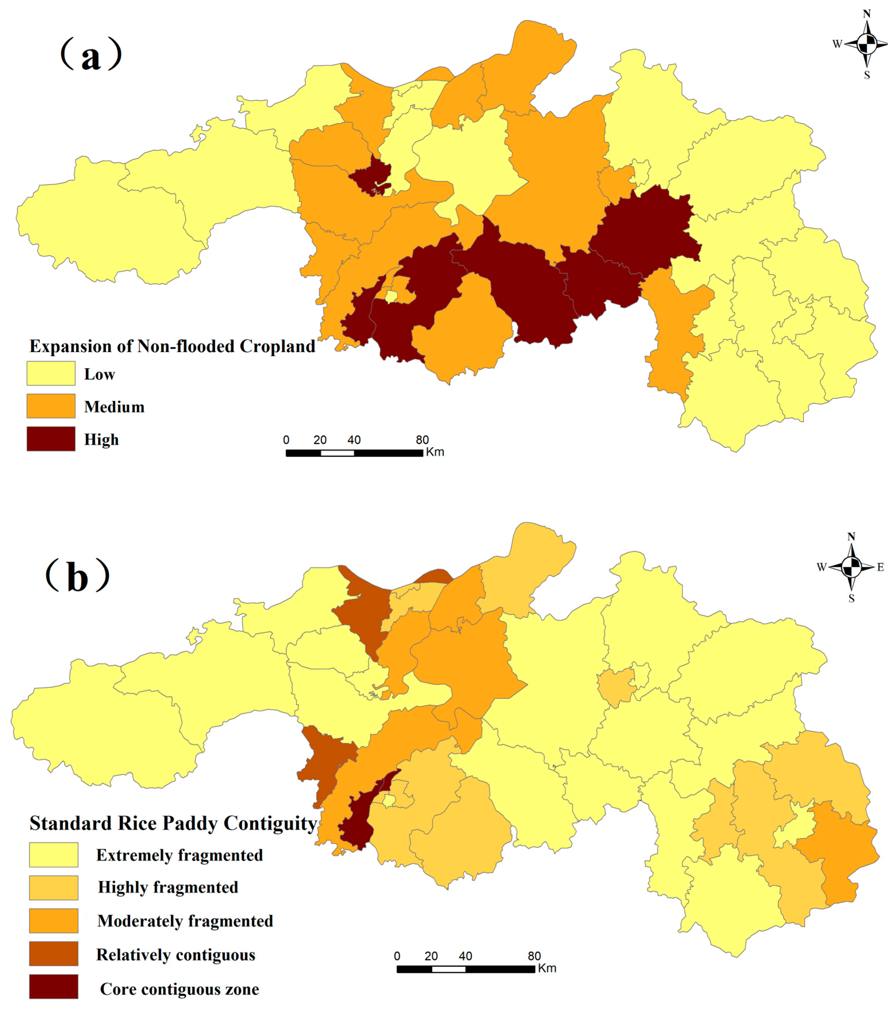
The spatial pattern of non-flooded cropland shifted from scattered distribution toward localized aggregation. In early periods, non-flooded cropland was often embedded as small patches within standard rice paddy landscapes, forming a mosaic pattern. Over time, some areas of non-flooded cropland gradually formed larger patches, suggesting the emergence of more clustered land-use patterns. This indicates that non-grain production risk is reflected not only in area expansion, but also in the weakening of paddy landscape connectivity and the basis for mechanized farming. The spatial patterns of non-flooded cropland expansion and standard rice paddy contiguity in 2020 are shown in Figure 5.
Figure 5.
Spatial patterns of non-flooded cropland expansion and standard rice paddy contiguity in 2020. (a) Expansion intensity of non-flooded cropland. (b) Contiguity of standard rice paddy.
4.6. Gravity Center Migration and Standard Deviation Ellipse Results
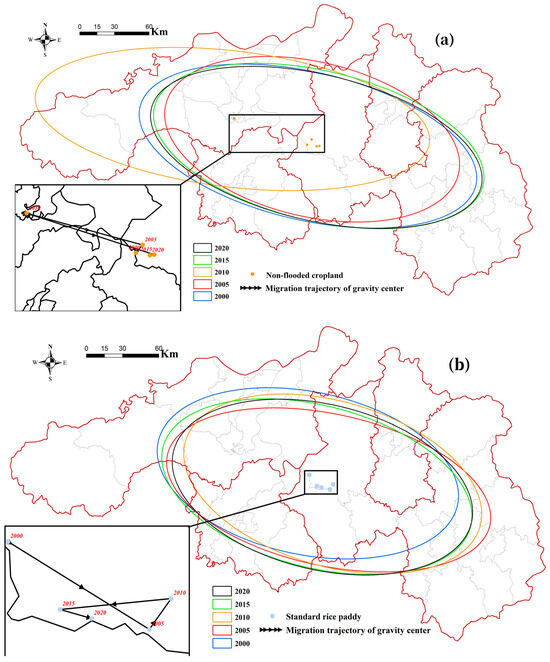
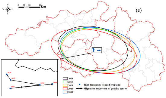
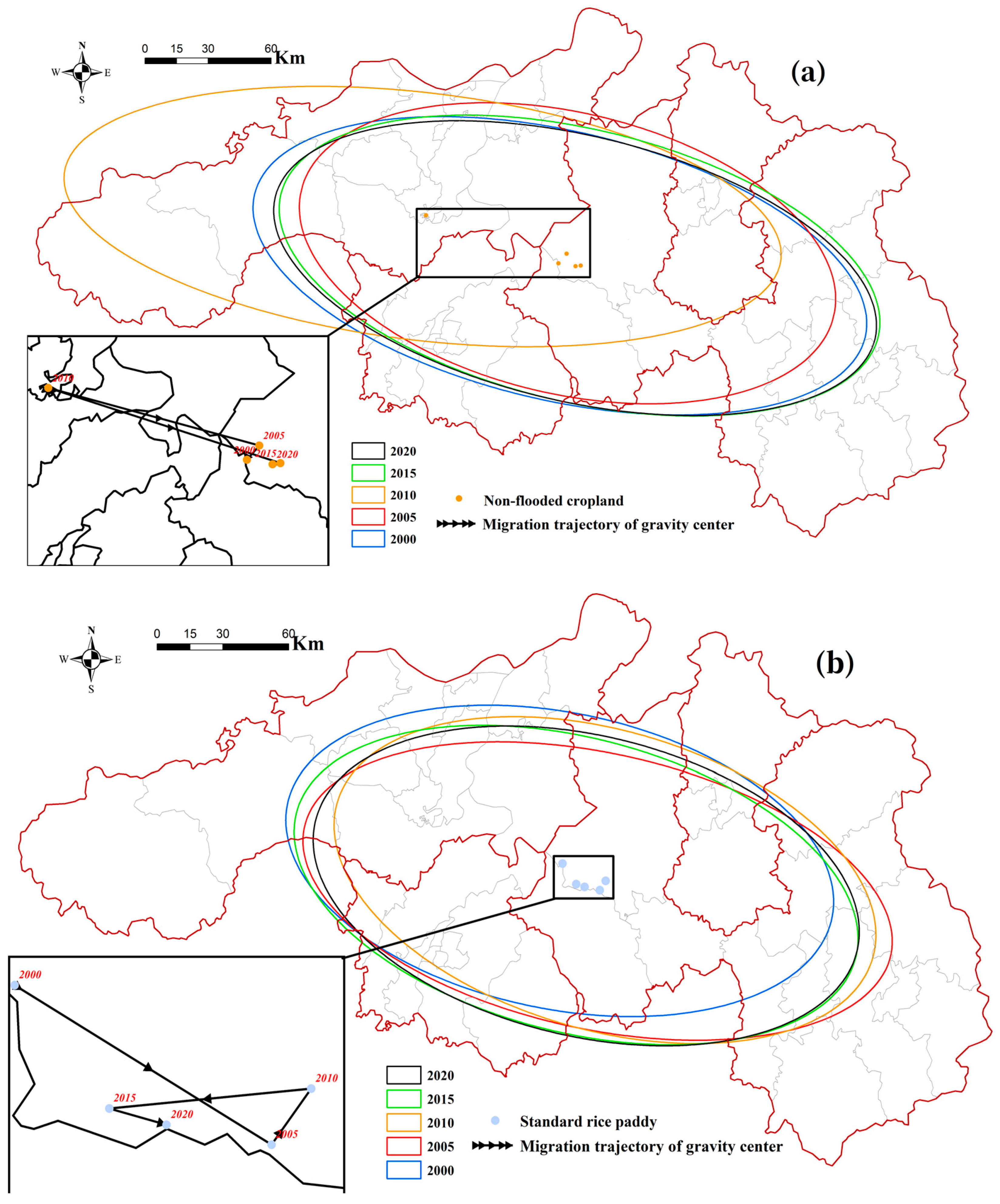
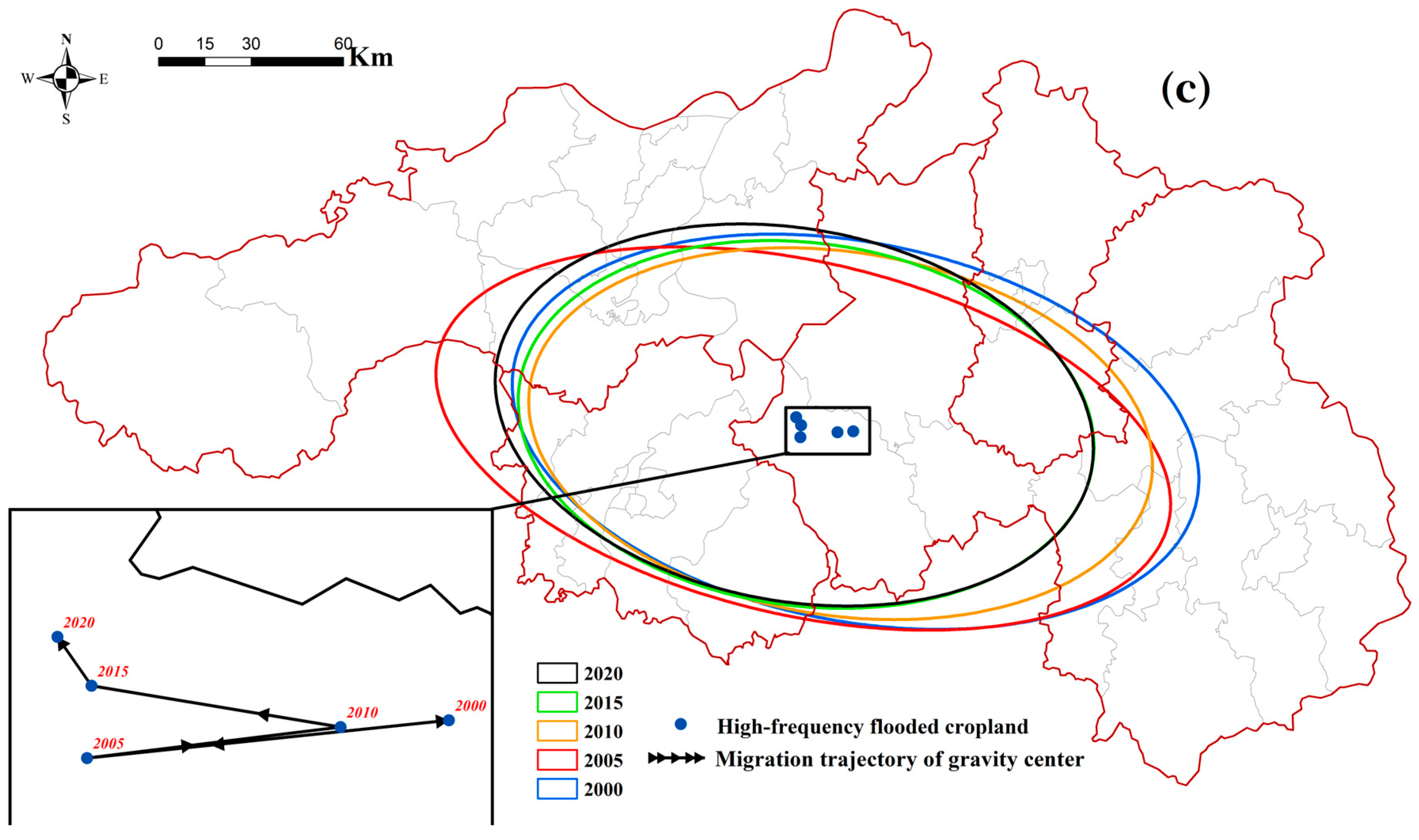
The gravity center and SDE results show that different cropland utilization systems followed distinct spatial trajectories. The gravity center of non-flooded cropland showed a directional shift during the study period, indicating that the spatial distribution of this class was not stable. In contrast, the gravity center of standard rice paddy remained more closely associated with traditional plain agricultural areas. These results describe broad spatial migration and dispersion patterns of the three cropland utilization types, but they should not be interpreted as direct evidence of socioeconomic driving mechanisms. The gravity center migration and standard deviation ellipses of the three cropland utilization types are shown in Figure 6.
Figure 6.
Gravity center migration and standard deviation ellipses of cropland utilization systems from 2000 to 2020. (a) Type 1 non-flooded cropland; (b) Type 2 standard rice paddy; and (c) Type 3 high-frequency flooded cropland. The ellipses describe broad spatial dispersion and directional trends rather than causal driving mechanisms.
The gravity center and SDE of high-frequency flooded cropland were more constrained by lake-area hydrological conditions. This category was more concentrated in low-lying areas around Poyang Lake, suggesting that its distribution was influenced not only by human management, but also by hydrological and geomorphological conditions.
4.7. Spatial Heterogeneity in the GWR Results
The diagnostic comparison between OLS and GWR models is presented in Table 3.
Table 3.
Diagnostic comparison between OLS and GWR models.
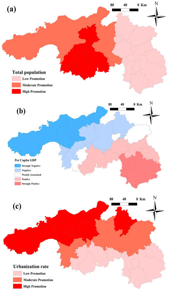
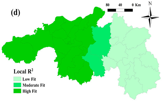
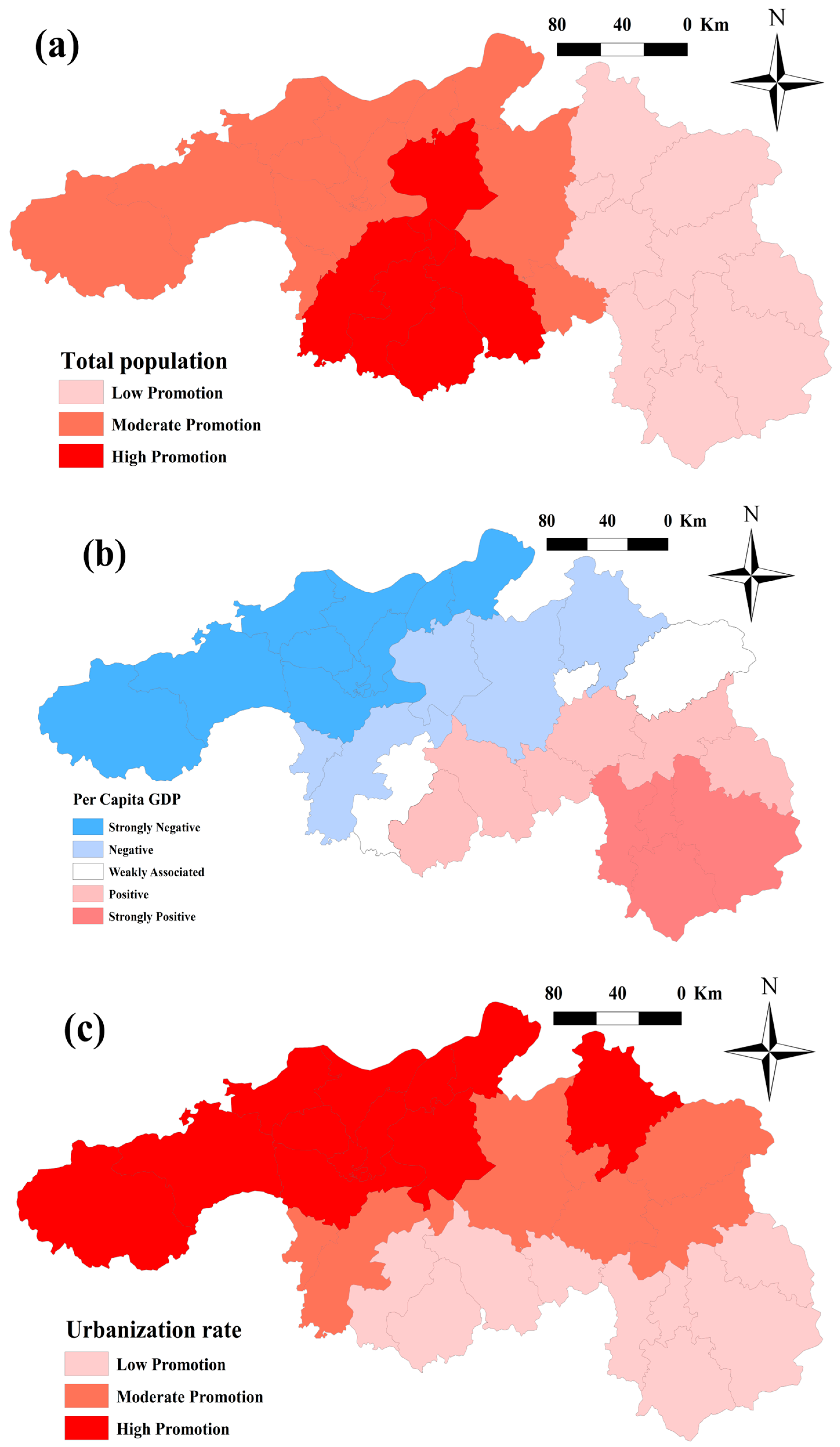
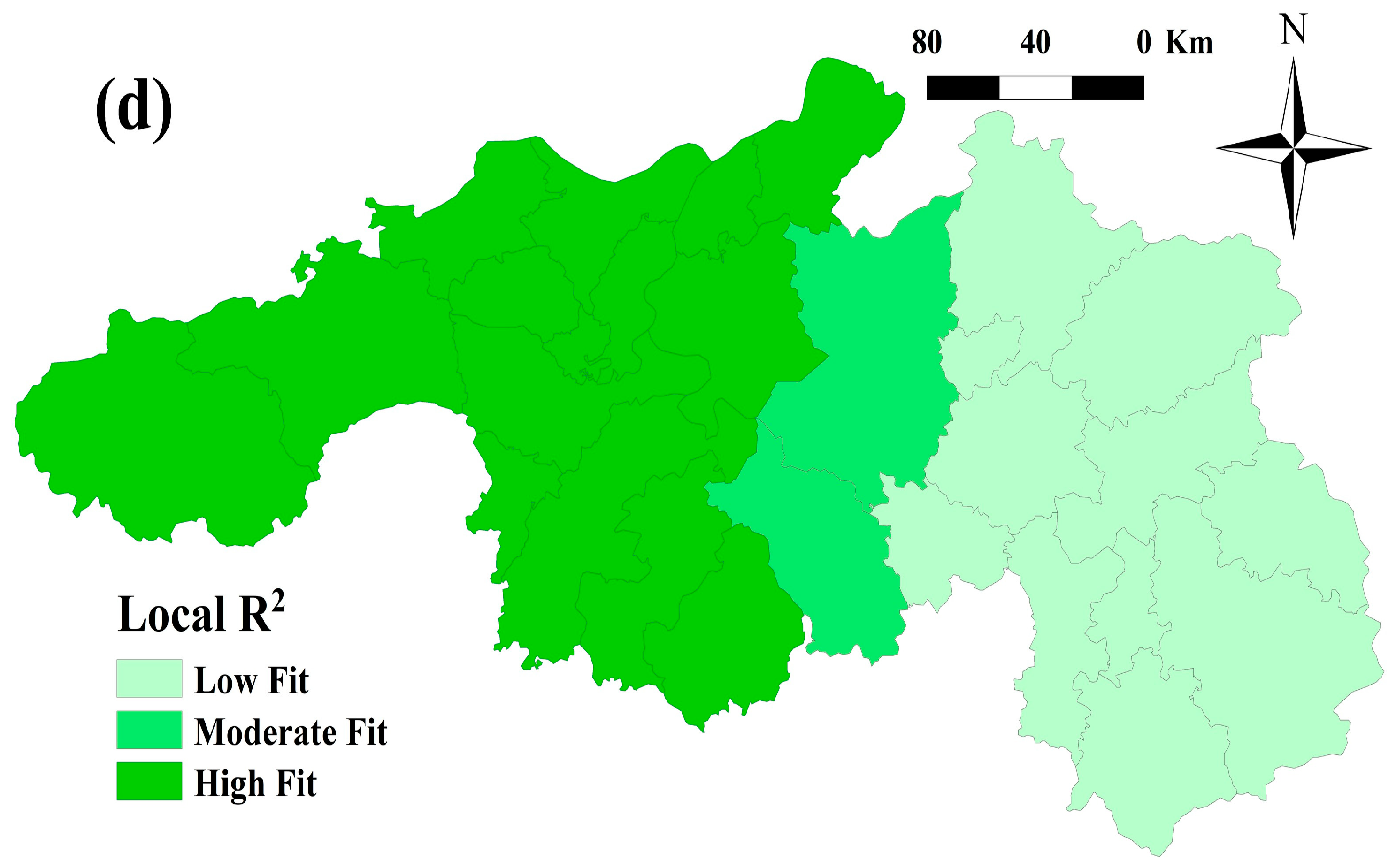
The GWR bandwidth determined by the AICc criterion was 57,876.63 and was used to construct the spatial weighting relationship in local regression. Compared with OLS, the GWR R2 increased from 0.020 to 0.185, and Sigma decreased from 0.184 to 0.181. These results indicate that incorporating spatial weights slightly improved the explanatory capacity and local fitting performance of the model. Nevertheless, the adjusted R2 values of both models were negative, and the AICc of GWR was not lower than that of OLS. The overall explanatory power of the model was therefore limited. Therefore, the GWR results were used only as auxiliary evidence for spatial heterogeneity and were not treated as the main basis for explaining the formation mechanism of non-flooded cropland. Accordingly, the GWR results were interpreted as exploratory evidence of spatial differences in socioeconomic associations rather than as strict causal evidence. The spatial distribution of the GWR coefficients and local R2 is shown in Figure 7.
Figure 7.
Spatial distribution of exploratory GWR results: (a) local coefficient of total population; (b) local coefficient of per capita GDP; (c) local coefficient of urbanization rate; and (d) local R2. The maps show county-level spatial associations rather than causal effects.
The local regression coefficients show that total population had coefficients close to zero, suggesting a weak direct association with changes in non-flooded cropland during 2005–2010. The coefficient of per capita GDP was weakly negative, ranging from approximately −2 × 10⁻⁶ to 0, indicating that non-flooded cropland expansion was not necessarily stronger in counties with higher economic development. The coefficient of urbanization rate was positive, ranging from approximately 0.0001 to 0.0036, suggesting a positive spatial association between urbanization level and non-flooded cropland change. This pattern implies that, during 2005–2010, urbanization may have been related to cropland structure adjustment, labor transfer, and changes in agricultural management.
5. Discussion
5.1. Applicability and Uncertainty of Phenology-Based Paddy System Identification
Beyond changes in cropland area, the results show that paddy landscape change was also expressed through patch fragmentation, reduced spatial continuity, and shifts in aggregation patterns. This indicates that landscape metrics provide information that conventional area-based land-use change analysis cannot fully capture. In particular, changes in PD, LPI, AI, and MPS help reveal whether standard rice paddy remains spatially continuous or becomes increasingly fragmented. Therefore, combining FF-based classification with landscape metrics allows the study to move from simple area monitoring toward a functional and structural interpretation of paddy landscape change.
This study used LSWI and EVI to construct annual FF and identify cropland utilization systems in Northern Jiangxi. Compared with single-date image classification, the phenology-based time-series approach better captured flooding signals during the rice transplanting period and was therefore suitable for cloudy and rainy regions in southern China. This result is consistent with previous rice-mapping studies showing that the LSWI–EVI relationship can effectively identify paddy flooding signals and that phenology-based methods are useful for mapping rice systems in complex humid landscapes [13,14,15]. The visual reliability assessment further suggested that the method could distinguish standard rice paddy from non-flooded cropland with reasonable stability.
Nevertheless, uncertainty remains. First, FF = 0 only indicates that no obvious flooding signal was detected during the year; it does not distinguish dry cropping, orchards, nursery stock, fallow land, abandoned cropland, or other non-rice uses. Second, FF ≥ 3 may result from rice-fishery integrated farming, continuous irrigation, or natural hydrological fluctuations, and cannot be equated with a single land-use type. Third, early Landsat imagery may be affected by cloud cover, limited valid observations, and Landsat 7 SLC-off gaps, which may bias FF statistics in some years. Therefore, the classification results should be interpreted as indicators of cropland flooding status and paddy-function change, rather than as precise crop-type classifications.
5.2. Expansion of Non-Flooded Cropland and Paddy Landscape Fragmentation
The results suggest a clear association between the expansion of non-flooded cropland and the fragmentation of standard rice paddy. When traditional paddy fields were converted to orchards, dry cropping, facility agriculture, or fallow land, formerly continuous paddy patches were fragmented into smaller and less connected units. This finding is consistent with studies showing that cropland change in China is increasingly reflected not only in area loss, but also in patch subdivision, reduced connectivity, and greater landscape fragmentation [11,16,17,18,19].
Compared with studies that focus mainly on cropland area loss, this study highlights the importance of paddy landscape structure. Even when the total area of standard rice paddy does not change dramatically, reductions in LPI and MPS may indicate a decline in contiguous core paddy fields and a weakening of mechanized farming conditions. This structural perspective complements previous non-grain production studies, which mainly emphasized the extent, spatial differentiation, and driving factors of non-grain production [7,8,9,10]. It also extends landscape-fragmentation research by linking patch-level structural change directly with paddy-function transformation and potential non-grain production risk [16,17,18,19].
5.3. Complementary Interpretation of County-Level Spatial Associations
The GWR analysis based on 2005–2010 cropland utilization changes and 2011 county-level statistics was used as a complementary exploratory analysis rather than as a major explanatory model. The results suggest weak but spatially heterogeneous county-level associations between socioeconomic variables and changes in non-flooded cropland. However, given the low overall explanatory power, negative adjusted R2 values, and the use of county-level aggregated variables, these findings should be interpreted only as preliminary spatial associations rather than evidence of socioeconomic driving mechanisms. Similarly to previous GWR-based studies, the spatial variation in local coefficients indicates that global regression results may conceal local differences in the association between socioeconomic context and cropland utilization change [20,21,22].
However, the overall explanatory power of the model was limited, and county-level analysis may be affected by MAUP and ecological fallacy. Thus, these results should be viewed as exploratory findings rather than causal conclusions. Future research should integrate household surveys, land-transfer data, and information on agricultural management entities to better clarify local processes associated with non-flooded cropland expansion and potential non-rice cultivation.
5.4. Implications for Paddy Landscape Management
Based on the observed changes in flooding-status classes, transition pathways, and landscape fragmentation metrics, this study provides several implications for paddy landscape monitoring and management.
The findings suggest that cropland monitoring and paddy landscape management should move beyond area-based control toward coordinated monitoring of cropland quantity, flooding-related function, and spatial configuration. In standard rice paddy concentration areas such as the Poyang Lake Plain and Gan-Fu Plain, contiguous paddy fields should be monitored and protected to reduce further fragmentation. In peri-urban areas, more refined monitoring and management mechanisms should be established to address the effects of rising land opportunity costs and capital investment in agriculture. In traditional agricultural areas affected by labor outflow, agricultural socialized services, mechanization support, and moderate-scale management may help reduce rice-production costs and encourage continued grain cultivation [2,3,4].
For high-frequency flooded cropland in lake areas, a balance should be maintained among food production, rice-fishery integrated farming, and ecological security. Although rice-fishery integrated farming can improve agricultural returns, excessive transformation may alter the basic function of paddy fields. Differentiated management should therefore be considered according to regional spatial characteristics and associated factors.
5.5. Research Limitations and Future Research
This study has several limitations. First, the 2010 GlobeLand30 cropland layer was used as a fixed baseline mask. This ensured spatial comparability across the 2000–2020 time series and focused the analysis on internal paddy-function and land-use structure changes within the baseline cropland extent. However, a single-year fixed mask may constrain the study extent. The mask comparison showed that the cropland areas in 2000, 2010, and 2020 were approximately 15,405.84 km2, 17,575.92 km2, and 16,270.91 km2, respectively, whereas the multi-year union mask area was approximately 19,810.58 km2. Compared with the 2010 fixed mask, the union mask increased the area by approximately 2234.66 km2, or 12.71%. Thus, some areas that existed as cropland in 2000 or 2020 may not have been included in the main analysis. The results are therefore most suitable for explaining internal land-use structure changes within the 2010 baseline cropland extent, rather than for providing a complete estimate of all cropland gains and losses across the entire study area. In addition, because landscape metrics are sensitive to spatial extent and boundary definition, the use of the 2010 fixed cropland mask may also influence patch number, patch size, and aggregation-related metrics. Therefore, the landscape-metric results should be interpreted as fragmentation patterns within the 2010 baseline cropland boundary rather than as complete fragmentation estimates for all cropland changes in Northern Jiangxi. Future studies should further adopt dynamic cropland masks or multi-year union masks to evaluate the influence of mask selection on classification, transition matrices, and landscape metrics. However, transition matrices and landscape metrics may still vary if a dynamic cropland mask or a full union-mask framework is used for all years. Therefore, the results should be interpreted as changes within a fixed baseline cropland extent, and future studies should further compare fixed, dynamic, and union-mask frameworks.
Second, the FF-based classification can identify flooding signals, but it cannot precisely distinguish the internal types of non-flooded cropland, such as dry cropping, orchards, nursery stock, fallow land, and abandoned cropland. The interpretation of non-grain production in this study should therefore be understood as potential non-rice or non-flooded cultivation risk, rather than as a strict crop-type classification.
Although the valid-observation statistics show that each observation year contained multiple usable Landsat observations, the mean number of valid observations per pixel differed among years. Such differences may affect the comparability of FF thresholds, especially in cloudy areas, Landsat 7 SLC-off affected periods, and lake–shore transition zones. Therefore, the FF-based classification should be interpreted as a relative flooding-status classification rather than an exact measure of annual irrigation frequency.
Third, the 30 m Landsat resolution may lead to mixed-pixel uncertainty, especially in fragmented peri-urban cropland and lake–shore transition zones. Limited high-resolution validation imagery for early years may also affect accuracy assessment. Because historical high-resolution imagery was incomplete for early years, especially 2000 and 2005, a fully independent quantitative accuracy assessment was not conducted. This limitation may affect the certainty of early-period classification results, although the use of Landsat false-color composites, stable neighboring-year features, topographic context, and paddy-field textures helped improve the plausibility of visual interpretation.
Classification uncertainty may propagate into downstream analyses, including transition matrices, landscape metrics, gravity center migration, SDE, and GWR. For example, confusion between non-flooded cropland and weakly flooded rice fields may affect estimated transition areas, while mixed pixels in fragmented peri-urban areas may influence patch number, patch size, and fragmentation metrics. Therefore, the transition and landscape-metric results should be interpreted as relative temporal and spatial patterns rather than exact measurements of crop-type conversion. Future studies should combine higher-resolution imagery, field survey data, and independent validation samples to quantify such uncertainty more explicitly.
Fourth, the GWR analysis was based on county-level statistics and may be affected by MAUP and ecological fallacy. Because county-level variables cannot directly represent household-level decision-making, the spatial analysis should be interpreted as exploratory. Future research should incorporate higher-resolution socioeconomic data, household surveys, and land-transfer information to further clarify the local processes associated with non-flooded cropland expansion and potential non-rice cultivation.
6. Conclusions
Using Northern Jiangxi as a case study, this research developed an EVI–LSWI–FF-based approach to classify cropland into non-flooded cropland, standard rice paddy, and high-frequency flooded cropland. The classification should be interpreted as a flooding-status and paddy-function classification rather than a precise crop-type map or direct identification of confirmed non-grain production.
The findings suggest that paddy systems in Northern Jiangxi experienced stage-based fluctuations. Standard rice paddy was concentrated in the Poyang Lake Plain and Gan-Fu Plain, which function as core grain-producing areas. Non-flooded cropland was mainly distributed along urban fringes, transport corridors, and hilly margins, while high-frequency flooded cropland was concentrated in low-lying lake areas. During 2010–2015, non-flooded cropland expanded substantially, standard rice paddy declined, and paddy landscape fragmentation intensified [2,4]. The expansion of non-flooded cropland suggests an increased risk of departure from conventional rice cultivation, rather than confirmed non-grain production at the crop-type level.
The landscape pattern analysis suggests that the expansion of non-flooded cropland affected not only cropland utilization types, but also paddy patch structure and spatial connectivity. Declines in the LPI and MPS of standard rice paddy indicate that core paddy patches were fragmented. The GWR results further suggest weak but spatially heterogeneous county-level associations between socioeconomic variables and non-flooded cropland change, although these associations should not be interpreted as causal explanations.
Overall, this study demonstrates the value of integrating phenology-based flooding-signal classification with landscape pattern analysis for monitoring paddy landscape change. By linking cropland utilization classes with transition pathways, fragmentation metrics, and exploratory spatial associations, the study provides a framework for identifying not only area changes but also functional and structural reorganization within paddy landscapes. These findings are most applicable to internal cropland utilization changes within the 2010 baseline cropland mask, and future studies should further verify the results using dynamic cropland boundaries, higher-resolution imagery, and more detailed socioeconomic data.
Supplementary Materials
The following supporting information can be downloaded at https://www.mdpi.com/article/10.3390/earth7040124/s1, Figure S1: Methodological workflow of this study; Table S1: Cropland mask pixel counts and areas used in this study; Table S2: Area comparison of cropland utilization systems under the 2010 fixed mask and the multi-year union mask; Figure S2: Temporal trends of Type 1, Type 2, and Type 3 areas under the 2010 fixed mask and the multi-year union mask; Table S3: Valid Landsat observations used for annual Flooding Frequency (FF) calculation.
Author Contributions
Conceptualization, H.-S.S. and X.H.; methodology, X.H.; software, X.H.; validation, H.-S.S. and X.H.; formal analysis, X.H.; investigation, H.-S.S. and X.H.; resources, H.-S.S.; data curation, X.H.; writing—original draft preparation, X.H.; writing—review and editing, H.-S.S. and X.H.; visualization, X.H.; supervision, H.-S.S.; project administration, H.-S.S. All authors have read and agreed to the published version of the manuscript.
Funding
This research received no external funding.
Data Availability Statement
The Landsat surface reflectance imagery and SRTM digital elevation model used in this study are publicly available through the Google Earth Engine platform. The GlobeLand30 land cover dataset is publicly available from the National Geomatics Center of China. Socioeconomic data were obtained from the Jiangxi Statistical Yearbook. The derived classification results, transition matrices, landscape metrics, and spatial analysis outputs generated during the study are available from the corresponding author upon reasonable request.
Acknowledgments
During the preparation of this manuscript, the authors used Gemini 3.1 Pro (Google LLC, Mountain View, CA, USA) and ChatGPT (GPT-5.5; OpenAI, San Francisco, CA, USA) for the purposes of English language refinement, manuscript formatting, reference checking, and improving the clarity of academic expression. The authors have reviewed and edited the output and take full responsibility for the content of this publication.
Conflicts of Interest
The authors declare no conflicts of interest.
Abbreviations
The following abbreviations are used in this manuscript:
| AI | Aggregation Index |
| EII | Expansion Intensity Index |
| EVI | Enhanced Vegetation Index |
| FF | Flooding Frequency |
| GEE | Google Earth Engine |
| GWR | Geographically Weighted Regression |
| LPI | Largest Patch Index |
| LSWI | Land Surface Water Index |
| MAUP | Modifiable Areal Unit Problem |
| MPS | Mean Patch Size |
| NGP | Non-Grain Production |
| OLS | Ordinary Least Squares |
| PD | Patch Density |
| SDE | Standard Deviation Ellipse |
| SRTM | Shuttle Radar Topography Mission |
| VIF | Variance Inflation Factor |
References
- Verburg, P.H.; Crossman, N.; Ellis, E.C.; Heinimann, A.; Hostert, P.; Mertz, O.; Nagendra, H.; Sikor, T.; Erb, K.-H.; Golubiewski, N.; et al. Land system science and sustainable development of the Earth system: A global land project perspective. Anthropocene 2015, 12, 29–41. [Google Scholar] [CrossRef] [Scilit]
- Zhang, D.; Yang, W.; Kang, D.; Zhang, H. Spatial-temporal characteristics and policy implication for non-grain production of cultivated land in Guanzhong Region. Land Use Policy 2023, 125, 106466. [Google Scholar] [CrossRef] [Scilit]
- Su, Y.; Qian, K.; Lin, L.; Wang, K.; Guan, T.; Gan, M. Identifying the driving forces of non-grain production expansion in rural China and its implications for policies on cultivated land protection. Land Use Policy 2020, 92, 104435. [Google Scholar] [CrossRef] [Scilit]
- Liu, J.; Kuang, W.; Zhang, Z.; Xu, X.; Qin, Y.; Ning, J.; Zhou, W.; Zhang, S.; Li, R.; Yan, C.; et al. Spatiotemporal characteristics, patterns, and causes of land-use changes in China since the late 1980s. J. Geogr. Sci. 2014, 24, 195–210. [Google Scholar] [CrossRef] [Scilit]
- Wang, L.; Xu, J.; Liu, Y.; Zhang, S. Spatial characteristics of the non-grain production rate of cropland and its driving factors in major grain-producing areas: Evidence from Shandong Province, China. Land 2023, 13, 22. [Google Scholar] [CrossRef] [Scilit]
- Yan, J.; Yang, Z.; Li, Z.; Li, X.; Xin, L.; Sun, L. Drivers of cropland abandonment in mountainous areas: A household decision model on farming scale in Southwest China. Land Use Policy 2016, 57, 459–469. [Google Scholar] [CrossRef] [Scilit]
- Zhang, Z.; Zheng, L.; Yu, D. Non-Grain Production of Cultivated Land in Hilly and Mountainous Areas at the Village Scale: A Case Study in Le’an County, China. Land 2023, 12, 1562. [Google Scholar] [CrossRef] [Scilit]
- Sun, Y.; Chang, Y.; Liu, J.; Ge, X.; Liu, G.-J.; Chen, F. Spatial Differentiation of Non-Grain Production on Cultivated Land and Its Driving Factors in Coastal China. Sustainability 2021, 13, 13064. [Google Scholar] [CrossRef] [Scilit]
- Zhao, S.; Xiao, D.; Yin, M. Spatiotemporal Patterns and Driving Factors of Non-Grain Cultivated Land in China’s Three Main Functional Grain Areas. Sustainability 2023, 15, 13720. [Google Scholar] [CrossRef] [Scilit]
- Ran, D.; Zhang, Z.; Jing, Y. A Study on the Spatial–Temporal Evolution and Driving Factors of Non-Grain Production in China’s Major Grain-Producing Provinces. Int. J. Environ. Res. Public Health 2022, 19, 16630. [Google Scholar] [CrossRef] [Scilit] [PubMed]
- Wang, X.; Hao, J.; Dai, Z.; Haider, S.; Chang, S.; Zhu, Z.; Duan, J.; Ren, G. Spatial-temporal characteristics of cropland distribution and its landscape fragmentation in China. Farming Syst. 2024, 2, 100078. [Google Scholar] [CrossRef] [Scilit]
- Nagendra, H.; Munroe, D.K.; Southworth, J. From being to becoming: Integrating methods for the study of land-cover change and landscape fragmentation. Environ. Plan. A Econ. Space 2004, 36, 2073–2092. [Google Scholar] [CrossRef] [Scilit]
- Xiao, X.; Boles, S.; Liu, J.; Zhuang, D.; Frolking, S.; Li, C.; Salas, W.; Moore, B. Mapping paddy rice agriculture in southern China using multi-temporal MODIS images. Remote Sens. Environ. 2005, 95, 480–492. [Google Scholar] [CrossRef] [Scilit]
- Dong, J.; Xiao, X.; Menarguez, M.A.; Zhang, G.; Qin, Y.; Thau, D.; Biradar, C.; Moore, B. Mapping paddy rice planting area in northeastern Asia with Landsat 8 images, phenology-based algorithm and Google Earth Engine. Remote Sens. Environ. 2016, 185, 142–154. [Google Scholar] [CrossRef] [Scilit] [PubMed]
- Ding, M.; Guan, Q.; Li, L.; Zhang, H.; Liu, C.; Zhang, L. Phenology-Based Rice Paddy Mapping Using Multi-Source Satellite Imagery and a Fusion Algorithm Applied to the Poyang Lake Plain, Southern China. Remote Sens. 2020, 12, 1022. [Google Scholar] [CrossRef] [Scilit]
- Yu, Q.; Hu, Q.; van Vliet, J.; Verburg, P.H.; Wu, W. GlobeLand30 Shows Little Cropland Area Loss but Greater Fragmentation in China. Int. J. Appl. Earth Obs. Geoinf. 2018, 66, 37–45. [Google Scholar] [CrossRef] [Scilit]
- Uuemaa, E.; Antrop, M.; Roosaare, J.; Marja, R.; Mander, Ü. Landscape Metrics and Indices: An Overview of Their Use in Landscape Research. Living Rev. Landsc. Res. 2009, 3, 1–28. [Google Scholar] [CrossRef] [Scilit]
- Uuemaa, E.; Mander, Ü.; Marja, R. Trends in the Use of Landscape Spatial Metrics as Landscape Indicators: A Review. Ecol. Indic. 2013, 28, 100–106. [Google Scholar] [CrossRef] [Scilit]
- Ai, J.; Yang, L.; Liu, Y.; Yu, K.; Liu, J. Dynamic Landscape Fragmentation and the Driving Forces on Haitan Island, China. Land 2022, 11, 136. [Google Scholar] [CrossRef] [Scilit]
- Fotheringham, A.S.; Brunsdon, C.; Charlton, M. Geographically Weighted Regression: The Analysis of Spatially Varying Relationships; John Wiley & Sons: Chichester, UK, 2002. [Google Scholar]
- Brunsdon, C.; Fotheringham, A.S.; Charlton, M.E. Geographically Weighted Regression: A Method for Exploring Spatial Nonstationarity. Geogr. Anal. 1996, 28, 281–298. [Google Scholar] [CrossRef] [Scilit]
- Fotheringham, A.S.; Charlton, M.E.; Brunsdon, C. Geographically Weighted Regression: A Natural Evolution of the Expansion Method for Spatial Data Analysis. Environ. Plan. A Econ. Space 1998, 30, 1905–1927. [Google Scholar] [CrossRef] [Scilit]
- Gorelick, N.; Hancher, M.; Dixon, M.; Ilyushchenko, S.; Thau, D.; Moore, R. Google Earth Engine: Planetary-scale geospatial analysis for everyone. Remote Sens. Environ. 2017, 202, 18–27. [Google Scholar] [CrossRef] [Scilit]
- Chen, J.; Chen, J.; Liao, A.; Cao, X.; Chen, L.; Chen, X.; He, C.; Han, G.; Peng, S.; Lu, M.; et al. Global land cover mapping at 30 m resolution: A POK-based operational approach. ISPRS J. Photogramm. Remote Sens. 2015, 103, 7–27. [Google Scholar] [CrossRef] [Scilit]
- Huete, A.; Didan, K.; Miura, T.; Rodriguez, E.P.; Gao, X.; Ferreira, L.G. Overview of the radiometric and biophysical performance of the MODIS vegetation indices. Remote Sens. Environ. 2002, 83, 195–213. [Google Scholar] [CrossRef] [Scilit]
- Olofsson, P.; Foody, G.M.; Herold, M.; Stehman, S.V.; Woodcock, C.E.; Wulder, M.A. Good practices for estimating area and assessing accuracy of land change. Remote Sens. Environ. 2014, 148, 42–57. [Google Scholar] [CrossRef] [Scilit]
- Congalton, R.G. A review of assessing the accuracy of classifications of remotely sensed data. Remote Sens. Environ. 1991, 37, 35–46. [Google Scholar] [CrossRef] [Scilit]
- McGarigal, K.; Cushman, S.A.; Ene, E. FRAGSTATS v4: Spatial Pattern Analysis Program for Categorical and Continuous Maps; University of Massachusetts: Amherst, MA, USA, 2012. [Google Scholar]
- Kumler, M.P.; Goodchild, M.F. The population center of Canada—Just north of Toronto. In Geographical Snapshots of North America; Janelle, D.G., Ed.; Guilford Press: New York, NY, USA, 1992; pp. 275–279. [Google Scholar]
- Lefever, D.W. Measuring geographic concentration by means of the standard deviational ellipse. Am. J. Sociol. 1926, 32, 88–94. [Google Scholar] [CrossRef] [Scilit] [PubMed]

Disclaimer/Publisher’s Note: The statements, opinions and data contained in all publications are solely those of the individual author(s) and contributor(s) and not of MDPI and/or the editor(s). MDPI and/or the editor(s) disclaim responsibility for any injury to people or property resulting from any ideas, methods, instructions or products referred to in the content. |
© 2026 by the authors. Licensee MDPI, Basel, Switzerland. This article is an open access article distributed under the terms and conditions of the Creative Commons Attribution (CC BY) license.