


Abstract
The spatial assessment of soil erosion drivers provides essential information for prioritizing soil conservation areas. This study aims to compare the performance of the Ordinary Least Squares (OLS) regression model and the Geographically Weighted Regression (GWR) model in explaining and analyzing the spatial variations of soil erosion in the Qara-Su watershed (Ardabil Province, Iran) and identifying the relative roles of the driving factors affecting erosion. To determine the relative importance of factors influencing soil erosion in the Qara-Su watershed, potential soil erosion (A) data and RUSLE model factors, including R, K, LS, C, and P, were collected at 13,845 points within the watershed. Initially, general relationships between erosion and contributing factors were examined using the OLS regression model. Subsequently, to analyze the spatial variability of relationships and identify the relative importance of factors at different locations within the watershed, the GWR model with an adaptive kernel and optimal bandwidth selection based on AICc was employed. The performance of the OLS and GWR models was compared based on fit indices such as R2 and Akaike Information Criterion corrected (AICc), and the relative importance of erosion factors was determined based on the mean local GWR coefficients. Results from the RUSLE model indicated an average annual soil erosion of approximately 7.64 tons per hectare, suggesting that the watershed falls into the moderate erosion risk category. According to the GWR model, significant improvements in explaining variations and reducing errors were observed, with higher R2 and adjusted R2 values (0.62 vs. 0.50) and lower AICc values (3687 vs. 97,848) compared to the OLS model. The local GWR coefficients confirmed spatial non-stationarity and revealed that LS (topography) has the highest importance in mountainous areas. The C factor showed a stronger protective effect in agricultural land-use areas. These results provide a basis for developing targeted strategies to mitigate and manage erosion drivers with higher relative importance and facilitate a better understanding of the causes and mechanisms of soil erosion across the watershed.
1. Introduction
1.1. Background
Soil erosion is one of the most significant environmental challenges worldwide, with widespread impacts on ecosystem stability, food security, and land productivity [1,2]. The erosion phenomenon leads to the degradation of soil structure, loss of nutrients, and a reduction in fertility, and on a larger scale, it causes secondary problems such as flooding, sedimentation in waterways, and decreased water quality. It is estimated that soil erosion moves approximately 75 billion tons of soil annually across the globe [3]. Among various types of erosion, water erosion has the largest extent, affecting about 1100 million hectares of land worldwide [4]. Therefore, monitoring and accurately estimating this type of erosion, along with identifying vulnerable areas for protective measures, is essential for the sustainable management of soil and water resources.
Recent advancements in remote sensing (RS) technologies and geographic information systems (GIS), along with quantitative models for estimating erosion, have enabled more precise analysis of environmental processes. Numerous models, including SWAT [5], WEPP [6], USLE [7], and RUSLE [8], have been developed for estimating soil erosion. Among these, the USLE and RUSLE models have been widely used at local and regional scales due to their simplicity, low cost, and reliability [1,7]. Despite their advantages, common erosion estimation models (such as RUSLE and USLE) primarily rely on the assumption of spatial uniformity in the relationships between influencing factors, treating environmental variables as consistent across the study area. This global approach, similar to Ordinary Least Squares (OLS) regression, overlooks spatial heterogeneity caused by variations in topography, climate, land use, and soil characteristics, leading to reduced accuracy in complex regions or areas with limited data [4,9,10]. This issue is particularly critical in heterogeneous agricultural-mountainous landscapes, where spatial variations are more pronounced, as global models fail to adequately represent local and spatially non-stationary relationships, often neglecting complex nonlinear and spatial heterogeneity [10,11]. To address this limitation, methods are needed that can reveal the spatial variability of the relationships between erosion factors. Geographically Weighted Regression (GWR), as an advanced spatial analysis approach, allows for local estimation of regression parameters, providing a more accurate representation of spatial heterogeneity and regional erosion patterns [7,10].
1.2. Literature Review
Numerous studies have been conducted on the spatial variations of soil erosion and sediment production in different regions worldwide. Li et al. [12] explored soil contamination and landscape patterns in the Pearl River Delta, China, using geographically weighted regression. They found stronger correlations between contamination and urban, water, and fragmented landscapes, while forest cover and distance from rivers reduced contamination. GWR outperformed OLS in capturing spatial variations. Zhu et al. [13] studied the effects of urbanization and landscape patterns on habitat quality in Hangzhou, China. They found a decline in habitat quality from 2004 to 2015, with suburban areas most affected. Urbanization had a negative impact, while landscape pattern effects varied across time and space. Mohammed et al. [14] compared OLS and GWR methods for predicting water erosion in the Dewana Basin, Iraq. They found that GWR outperformed OLS by accounting for local variations, while no significant relationship was found between erosion and slope degree. The Bergsma method was also less accurate than GWR. The Bergsma method refers to an empirical field-based approach developed by Bergsma [15,16] for evaluating erosion intensity and soil erodibility through observation and classification of microtopographic erosion features (e.g., rills, pedestals, root exposure) on arable fields or slopes, often used as a qualitative or semi-quantitative alternative or complement to nomograph-based K-factor estimation in areas with limited soil data.
The GWR enables better capture of varying spatial processes in heterogeneous environments [17]. The MGWR approach showed strong performance in explaining spatial variability.
Yu et al. [18] examined the impact of land use/cover change on soil erosion in Changwu County on the Loess Plateau, China. Using remote sensing data and the RUSLE model, they assessed erosion changes over a 30-year period. The results indicated marked land use transformations and a rising trend in average annual soil erosion, with spatial lag and spatial error models providing the best performance. Yao et al. [19] examined soil erosion in the Jihe Basin, China, with the aim of identifying its key drivers. Using the RSEM and MGWR models, they found that slope plays the dominant role in controlling erosion, while vegetation cover has a mitigating effect. Multiscale Geographically Weighted Regression (MGWR) is an advanced extension of standard GWR that allows each explanatory variable to operate at its own optimal spatial scale by assigning individual bandwidths, rather than a single bandwidth for all variables.
Karolinoerita et al. [20] investigated soil erosion drivers in the Central Citarum Watershed, West Java, Indonesia. Using an MGWR model, they aimed to identify the main factors controlling erosion patterns. The results showed high annual soil erosion, largely governed by slope conditions and vegetation cover, with MGWR outperforming OLS and GWR models. Chuenchum et al. [21] integrated USLE with GWR in the Nazas-Rodeo basin in Mexico to evaluate the spatial changes in the relative importance of erosion factors. GWR showed significant improvements over OLS, identifying more than 60% of the basin as areas with high erosion potential. Mirchooli et al. [9] in Iran used the RUSLE model along with GIS and remote sensing data to identify soil erosion and its sensitive areas in the Talār basin. Their study employed spatial statistical methods such as OLS and GWR to analyze the relationships between erosion factors and land use changes. The results indicated the presence of spatial non-stationarity, with GWR showing better predictive ability compared to OLS, as indicated by higher R2 and lower Akaike Information Criterion corrected (AICc) values. Li et al. [22] demonstrated that spatial–temporal non-stationarity limits the OLS model’s ability to calibrate the Soil Loss Equation, while advanced Geographically Weighted Regression (GWR) methods using UAV data improved accuracy in the Caidian region. Similarly, Peng et al. [10] applied GWR in Ethiopia’s Gubalafto region, result that erosion was most intense on steep, sparsely vegetated slopes near drainage channels, confirming significant spatial heterogeneity in erosion drivers.
According to the literature, across diverse environments globally, researchers have consistently found that the influence of key factors like slope, vegetation cover, and land use is not uniform but changes from one location to another. Furthermore, beyond demonstrating superior model fit, the spatially explicit outputs of GWR (e.g., maps of local coefficients and local R2) have been effectively applied to guide specific conservation measures. Studies have used these outputs to precisely delineate priority areas for mechanical interventions like terracing (where LS-factor influence is locally highest) and for biological measures such as reforestation or cover cropping (where C-factor influence is most detrimental), thereby optimizing the allocation of limited conservation resources [7,9,10]. Despite the proven strength of GWR, most comparisons are conducted in basins with distinct climates, topographies, or land-use systems, there is a lack of research that explicitly compares OLS and GWR within the specific context of a heterogeneous, mountainous-agricultural watershed in northwest Iran. The Qara-Su watershed in Ardabil Province stands out due to its pronounced biophysical heterogeneity, including steep topographic gradients (elevation 1200–4788 m, slopes up to >22% in margins), heterogeneous lithology (resistant sedimentary rocks upstream vs. erodible Quaternary deposits downstream), variable precipitation erosivity, and rapid land-use shifts (notably rangeland/forest decline and agriculture/urban expansion over recent decades). These factors generate spatially non-stationary relationships in erosion drivers, which global models like standard RUSLE or prior local assessments (e.g., AHP-Fuzzy zoning of erosion potential based on land-use changes) often overlook, leading to generalized rather than targeted conservation recommendations. By applying GWR alongside OLS, this study fills a critical gap in northwestern Iran’s mountainous-agricultural watersheds: it quantifies and maps local variations in RUSLE factor importance (e.g., topographic LS dominance in southwestern highlands, protective C effects in central agricultural zones), thereby providing spatially explicit guidance for cost-effective, location-specific interventions that enhance soil conservation efficiency amid ongoing environmental pressures. The research will not only test the established superiority of GWR in this new setting but will also map the spatial variation of local regression coefficients to identify exactly where and how much each environmental factor contributes to erosion risk across the landscape. This will provide crucial, location-specific indications that can directly inform targeted land management and conservation strategies for this ecologically and economically important watershed in Northwest Iran.
1.3. Scope and Objective
To compare Ordinary Least Squares (OLS) and Geographically Weighted Regression (GWR) models for explaining the spatial pattern of soil erosion, numerous studies have indicated the superiority of GWR in identifying the spatial heterogeneity of relationships between erosion factors and its rate. These studies indicate that OLS assumes uniform relationships across the entire region, while GWR provides higher accuracy in heterogeneous areas such as mountainous regions by locally estimating parameters. The Qara-Su watershed in Ardabil Province was selected for this research due to its regional significance and environmental heterogeneity, which facilitate advanced spatial analyses. As the longest and most water-abundant river in the province, the Qara-Su constitutes a major hydrological system.
The Qara-Su watershed in Ardabil province is important for study due to its mix of agricultural, industrial, and tourism activities, along with population centers and protected areas affected by human impact [23]. Steep, sparsely vegetated mountains with sensitive geology are prone to severe erosion, a risk that has been significantly intensified by human activities like overgrazing and unsuitable farming [24]. Critically, the study area features a heterogeneous mountainous-urban landscape characterized by steep topographic slopes, diverse land uses, and areas of significant human pressure. This pronounced spatial variability provides a key prerequisite for testing the GWR model against the global OLS approach, as it ensures the likely presence of spatial non-stationarity in erosion drivers. Furthermore, existing studies in the sub-watersheds of this region have identified soil erosion as a critical variable affecting ecological quality, confirming the area’s relevance for conservation-focused research. Environmental concerns, including pollution in the river’s urban sections, show the practical importance of developing directed soil conservation strategies for this basin.
Given the heterogeneous topography, extensive land-use changes, poor vegetation cover in upstream areas, and moderate to severe erosion in the Qara-Su watershed of Ardabil Province, common soil erosion regression models like RUSLE, which are based on the assumption of uniform spatial relationships, fail to adequately explain the severe spatial heterogeneity of relationships between influencing factors. Consequently, this reduces the accuracy of predictions and the prioritization of sensitive areas. This limitation is particularly challenging for targeted conservation planning in mountainous–agricultural watersheds like Qara-Su, where high sediment yield, reduced soil fertility, and flood risk are prevalent. Therefore, the present study aims to compare the performance of the OLS and GWR models in analyzing the spatial pattern of soil erosion. It seeks to provide a more localized and precise approach for identifying spatially non-stationary relationships among influential factors, thereby supporting the sustainable management of soil and water resources in this watershed.
2. Materials and Methods
2.1. Description of the Study Area
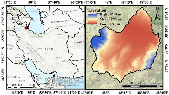
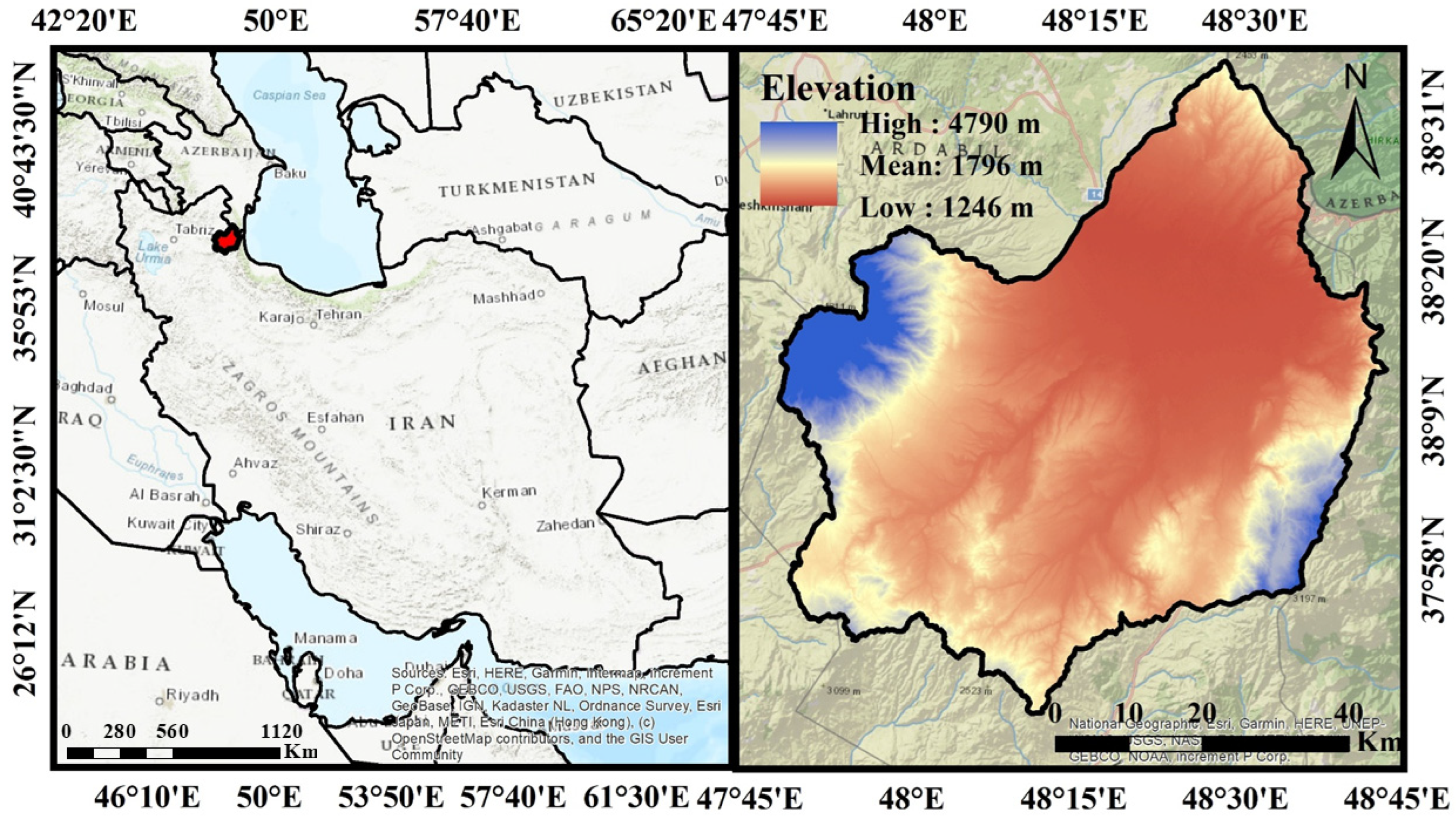
The Qara-Su watershed, covering approximately 4861 square kilometers, is a key hydrological basin in Ardabil Province in northwestern Iran (Figure 1). The watershed comprises the Qara-Su River as the main tributary of the Aras River, along with sub-watersheds such as Quri-Chay and Neor. Elevation ranges from approximately 1200 m in the downstream areas to over 4200 m (with a maximum of 4788 m) in the highlands, with an average slope ranging between 16.49% and 22.4%, and the steepest slopes located in the eastern and western parts. The mean annual precipitation is about 351.52 mm [25].
Figure 1.
Geographic location of the Qara-Su watershed in Ardabil Province and northwestern Iran.
The dominant soil types in the Qara-Su watershed, according to USDA Soil Taxonomy, are Inceptisols, Rock Outcrops/Inceptisols, Rock Outcrops/Entisols, Entisols, and Aridisols. Equivalent World reference base for soil resources (WRB) (2023) classes include mainly Cambisols, Regosols, Leptosols, and Calcisols [26]. These soils reflect the basin’s steep topography, sedimentary lithology upstream, and alluvial deposits downstream, contributing to variable erodibility across the watershed.
Based on the 1:100,000 geological maps of Ardabil, the investigation site contains diverse rock and sediment facies dating from the Mesozoic and Cenozoic eras [27].
Geologically, the basin consists predominantly of sedimentary formations, including limestone, sandstone, and Quaternary deposits. The upstream areas feature more resistant lithologies (limestone and sandstone), while the downstream sections comprise more erodible materials (silty-clay and alluvial deposits). This heterogeneous lithology, combined with steep slopes, plays a significant role in exacerbating soil erosion [28].
The study area’s varied land uses and heterogeneous topography make it highly susceptible to soil erosion, with floods and sediment production posing a major problem for agricultural and rangeland activities [29].
2.2. Research Methodology
2.2.1. Estimation of Erosion Using the RUSLE Model
To estimate the potential soil erosion in this study, the Revised Universal Soil Loss Equation (RUSLE) (Equation (1)) was employed. This model integrates five primary factors: rainfall erosivity (R), soil erodibility (K), the topographic factor (LS), cover management (C), and support practice (P) [30]. The topographic and terrain characteristics of a landscape (such as its slope, aspect, and elevation) play a crucial role in shaping critical soil processes, including drainage, runoff, temperature dynamics, formation, and erosion [31]. Input data for the model included meteorological records (precipitation and temperature), hydrological data, soil texture maps, geological maps, a Digital Elevation Model (DEM), land use maps, and Google Earth imagery.
The rainfall erosivity (R) factor was calculated using precipitation data and regional rainfall maps according to Equation (2) to quantify the impact of rainfall energy on erosion [32]. Due to the lack of high-resolution storm intensity data, the rainfall erosivity (R) factor was estimated using an established empirical relationship based on mean monthly precipitation (Equation (2)). This is a common proxy when direct intensity measurements are unavailable [33]. Rainfall Erosivity (R): Calculated using monthly precipitation data from synoptic and rain-gauge stations in/near the Qara-Su watershed (Ardabil Province Meteorological Organization), covering a 41-year period (1981–2022). Missing values (<5%) were imputed by linear temporal interpolation or IDW spatial interpolation in ArcGIS (version 10.8). Soil erodibility (K) was determined based on physical soil properties, including texture and organic matter content [34]. The soil erodibility (K) factor was determined based on physical soil properties, including texture, structure, permeability, and organic matter content [34]. The soil erodibility (K) factor was derived from available soil texture maps, land-use classes, and Curve Number (CN) as an indicator of hydrologic soil group and permeability [35,36]. K values were assigned according to standard tables [37], for the dominant soil-hydrologic combinations and mapped using GIS overlay of texture and land-use layers. Soil organic matter was accounted for through standard K values assigned from published nomograph tables for dominant soil–hydrologic combinations in northwestern Iran [37]; no new field sampling or laboratory analysis of soil organic carbon was conducted due to the large watershed area and reliance on validated secondary data.
The topographic (LS) factor was derived by processing the DEM to calculate slope length and steepness in accordance with Equation (3) [38]. The topographic (LS) factor was derived from a 30 m DEM with multiple flow directions in ArcGIS (version 10.8). The cover management (C) factor was obtained using an NDVI map generated from Landsat 8 imagery and remote sensing processing, following Equation (4) [39]. The 30 m resolution Landsat 8 OLI image from 5 June 2024 was processed in TerrSet software (version 19.0.7) to derive the NDVI-based C factor representative of peak vegetation conditions. The NDVI was extracted from a Landsat 8 (OLI sensor) satellite image (Path/Row: 166/34) acquired on 5 June 2024, corresponding to the peak vegetation season. The image was sourced from the United States Geological Survey (USGS) EarthExplorer platform. The vegetation cover factor (C) was then calculated using the established empirical relationship which is presented as Equation (4).
The support practice (P) factor, which represents the erosion-reducing effect of conservation practices such as terracing and contour farming, was assigned based on land use maps and slope [34]. The land use map was prepared using a Landsat 8 (OLI/TIRS) image from 5 June 2024, acquired from the USGS. The image underwent radiometric and geometric correction in ENVI software (version 5.6). Supervised classification using the Maximum Likelihood algorithm was then performed to define land use classes (e.g., dry/irrigated farmland, residential, rangeland, water, rock outcrop). The final map was refined in ArcGIS (version 10.8) (e.g., noise removal, smoothing), and its accuracy was assessed using Google Earth imagery. The classification accuracy was formally assessed according to Congalton & Green [40], with the overall accuracy and Kappa coefficient reported.
All these factor layers were integrated using raster-based analyses in the ArcGIS (version 10.8) environment to produce the final spatial distribution map of soil erosion.
2.2.2. Determining the Relative Importance of Soil Erosion Factors
To determine the relative importance of factors influencing soil erosion in the Qara-Su watershed, analyses were initially conducted separately for 27 sub-watersheds. However, due to the limited number of observations in some sub-watersheds and insufficient spatial neighborhoods for stable estimation of local parameters, implementing the GWR model at the sub-watershed scale encountered issues such as model instability and neighbor deficiency error [10]. To overcome this limitation, the raster layer of potential soil erosion (A) was first converted to point data, generating a total of 13,845 points across the entire watershed to appropriately sample spatial heterogeneities. For each point, the values of potential soil erosion (A) and the RUSLE model factors (R, K, LS, C, and P) were extracted using the ArcGIS (version 10.8) environment. The 13,845 points were generated by converting the potential soil erosion (A) raster layer to vector points using the ‘Raster to Point’ tool in ArcGIS (version 10.8). This method creates one point at the center of each raster cell (30 m resolution), systematically covering the entire watershed. This was not a random or stratified sample, but a deterministic and exhaustive conversion. This approach was chosen to preserve the full spatial resolution and heterogeneity of the original RUSLE output and to provide a complete, spatially continuous dataset necessary for stable local parameter estimation in the GWR model.
To assess the relative importance of erosion factors, two regression models were employed. First, the OLS model, as a global model, was executed with A as the dependent variable and the RUSLE factors as independent variables to examine the general relationships between the variables [41]. Multicollinearity among the explanatory variables was evaluated using the Variance Inflation Factor (VIF). Subsequently, the GWR model was applied to investigate the spatial variability of the relationships between the variables. An adaptive kernel was used in this model, and the optimal bandwidth was determined based on minimizing the corrected Akaike Information Criterion corrected (AICc). The performance of the OLS and GWR models was compared based on fit indices, including AICc and the coefficient of determination (R2) [42]. The relative importance of soil erosion factors was determined based on the mean local coefficients obtained from the GWR model, and maps of local coefficients and local R2 were prepared to visualize the spatial pattern of relationship variations.
2.2.3. The OLS Regression Model Application
The OLS regression model is a global approach that assumes the relationships between independent and dependent variables are constant and uniform across the entire study area. In this analysis of the relative importance of soil erosion factors in the Qara-Su watershed, the model takes the soil erosion (A) calculated by the RUSLE model as the dependent variable and the R, K, LS, C, and P factors as independent variables. OLS fits a single regression equation for all spatial units, providing constant coefficients (β) that represent the average effect of each factor across the entire basin. While this model is simple, interpretable, and serves as a baseline for comparison with local models, it cannot identify spatial non-stationarity in relationships within heterogeneous regions like Qara-Su, which may reduce prediction accuracy [9,43]. The application of OLS for soil erosion with the RUSLE model is presented as Equation (5):
where is soil erosion and the remaining terms are the RUSLE factors. The β coefficients are estimated by minimizing the sum of squared errors.
2.2.4. The GWR Model Setting
The GWR model is an advanced local technique that allows the relationships between erosion factors and its magnitude to vary across space. This model fits a separate regression equation for each spatial unit (e.g., homogeneous units within the Qara-Su watershed), assigning greater weight to closer neighboring points. The optimal bandwidth is determined using an adaptive method and the AICc criterion. Local coefficients (β(ui,vi)) enable the mapping of spatial variations in the importance of RUSLE factors and provide a better description of spatial heterogeneity. Studies indicate that GWR offers higher accuracy (greater R2 and lower AICc) compared to OLS and is useful for prioritizing conservation actions in heterogeneous regions [7,10,44].
The GWR model was executed using the Geographically Weighted Regression tool in the ArcGIS (version 10.8) Spatial Statistics toolbox. An adaptive kernel type was employed to account for varying point density across the watershed. The optimal bandwidth (defining the spatial scale of local relationships) was automatically determined by minimizing the corrected Akaike Information Criterion (AICc), a standard approach that balances model fit and complexity to prevent overfitting [41]. This process yielded an optimal adaptive bandwidth of 1000 nearest neighbors, which was used for the final analysis.
The model is formulated as Equation (6):
where is the soil erosion rate at land unit i; are the geographical coordinates of land unit i; is the intercept and is the slope (coefficient) of the GWR model at land unit i; k is the number of independent variables; are the independent variables (in this case, the R, K, LS, and C factors for each land unit); and is the random error at each land unit.
3. Results and Discussion
3.1. Erosion Modeling
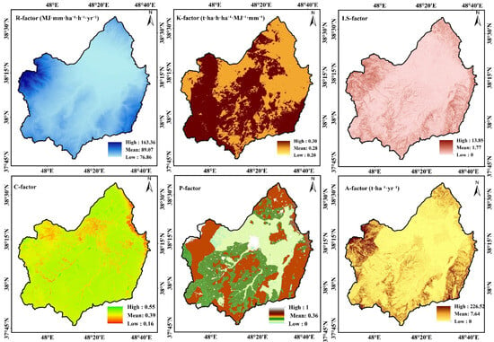
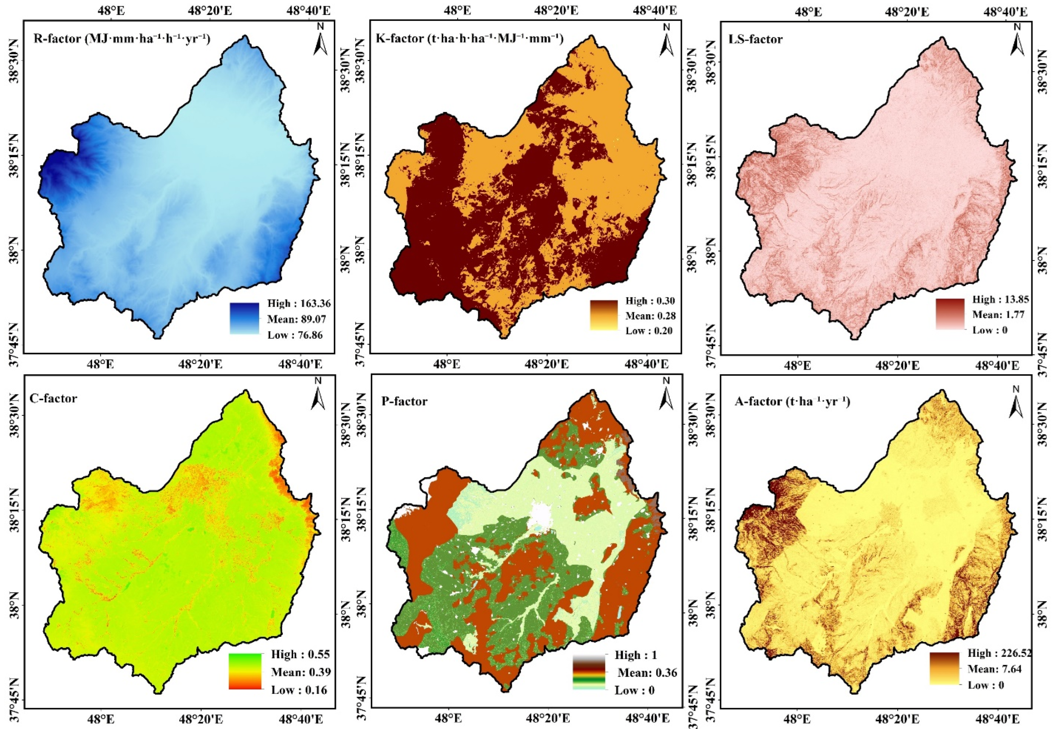
Figure 2 presents the results of the RUSLE model, illustrating the spatial pattern of factors influencing soil erosion in the Qara-Su watershed.
Figure 2.
Spatial distribution of the RUSLE model factors in the Qara-Su watershed.
The results of the RUSLE model (Figure 2) indicated that the average R-factor in the Qara-Su watershed is approximately 89.07 MJ·mm·ha−1·h−1·y−1, reflecting moderate rainfall erosivity at the basin scale. The average K-factor was found to be 0.28 t·ha·h·ha−1·MJ−1·mm−1, indicating a relatively high susceptibility of the region’s soils to erosion. The LS-factor was estimated with a mean of 1.77, confirming the prominent role of topographic conditions and slope in exacerbating soil erosion across the watershed. The C-factor results suggest moderate vegetation cover conditions and a notable influence of land use on soil erosion. Additionally, the support practice P-factor, with a mean of 0.36, shows the limited yet significant effect of conservation measures in reducing soil erosion. According to the results, the mean annual soil erosion estimated by the RUSLE model for the Qara-Su watershed is about 7.64 t·ha−1·y−1, placing the basin in the moderate erosion class.
The mean annual soil erosion in the Qara-Su watershed (7.64 t·ha−1·y−1) aligns with results from similar studies in watersheds of northwestern Iran and semi-arid regions. For instance, Korkanc et al. [45] obtained a slightly higher average of 9.1 t·ha−1·y−1 in the neighboring Gorganrood watershed, attributable to steeper slopes and greater rangeland degradation. Compared to the study by Namdar [38] in the Qara-Su watershed, which reported a rate of 5.8 to 10.4 t·ha−1·y−1 with a focus on land use changes, the present value falls within this range, confirming that the conversion of rangelands to agricultural lands and the topographic (LS) factor are primary drivers of moderate erosion in this region.
3.2. The OLS Regression Model Results
The OLS linear regression model was applied to 13,845 randomly distributed points across the studied watershed. The dependent variable was the annual soil erosion rate (A) calculated from the RUSLE equation, and the independent variables included the R, K, LS, C, and P factors. Table 1 presents the results of the OLS regression model for the factors affecting soil erosion in the Qara-Su watershed.
Table 1.
Results of the OLS regression model for factors affecting soil erosion in the Qara-Su watershed.
The OLS regression model indicated a strong relationship between soil loss (A) and the RUSLE factors. The model explained approximately 49.6% of the variance in soil loss (R2 = 0.496; Adjusted R2 = 0.496), demonstrating stable model performance. The model was overall highly significant (p < 0.01), as confirmed by the joint F and Wald tests. The corrected Akaike Information Criterion (AICc) was 97,848.26, which can serve as a baseline for comparison with explicit spatial models. Among the explanatory variables, the R, LS, and P factors showed a statistically significant positive relationship with soil loss (Robust p < 0.01). In contrast, the K and C factors did not show a significant relationship with soil loss. The Variance Inflation Factor (VIF) values for all variables were significantly below the critical threshold of 7.5, indicating the absence of multicollinearity among the explanatory variables. However, the Koenker (BP) test was significant (p < 0.01), suggesting the presence of spatial non-stationarity, or in other words, heteroscedasticity in the relationships.
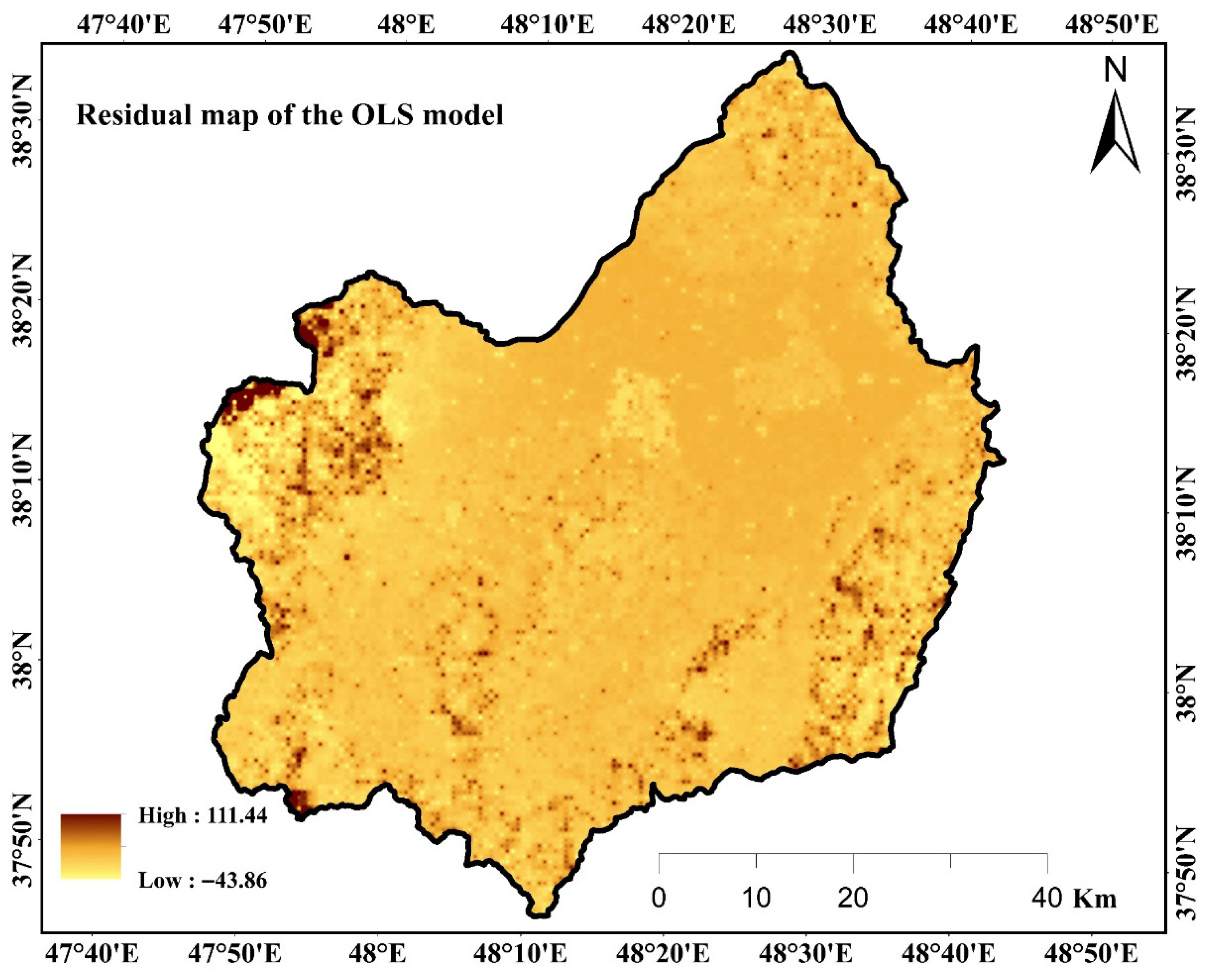
The spatial distribution of residuals from the OLS regression model in the Qara-Su watershed is presented in Figure 3.
Figure 3.
Spatial distribution of residuals from the OLS regression model in the Qara-Su watershed.
The residual map from the OLS model (Figure 3) reveals a clear spatial pattern in prediction errors. Positive residuals are concentrated in the eastern and southwestern parts of the watershed, indicating a significant underestimation of soil erosion by the OLS model in these areas. In contrast, negative residuals (reaching up to approximately −44 t·ha−1·y−1) are scattered across the northern and central fringes, suggesting an overestimation of erosion in these regions. This clustered, non-random pattern of residuals, combined with the significance (p < 0.01) of the Koenker (BP) test, confirms the presence of strong spatial non-stationarity in the relationships between the RUSLE factors and soil erosion.
3.3. The GWR Model Results
The effectiveness of the GWR model in capturing spatial non-stationarity was evaluated using a suite of diagnostic indicators. Globally, the GWR model showed a substantial improvement over the OLS model, with the coefficient of determination increasing from 0.50 to 0.62 and the corrected Akaike Information Criterion (AICc) decreasing dramatically from 97,848 to 3687 (Table 2). The effective number of parameters (9.63) and the residual standard deviation (Sigma = 20.35) further describe the model’s parsimonious local fitting. Crucially, the spatial map of local R2 values (Figure 4f) demonstrates that the model’s explanatory power varies geographically, with maxima (~0.61) in central and southwestern areas, directly visualizing the addressed heterogeneity. This is corroborated by the reduction in the spatially clustered residuals evident in the OLS model (Figure 3). Collectively, these diagnostics confirm that the GWR model successfully managed the spatial non-stationarity in the relationships between erosion drivers.
Table 2.
Goodness-of-fit indices for the OLS and GWR models in soil erosion estimation.
Figure 4.
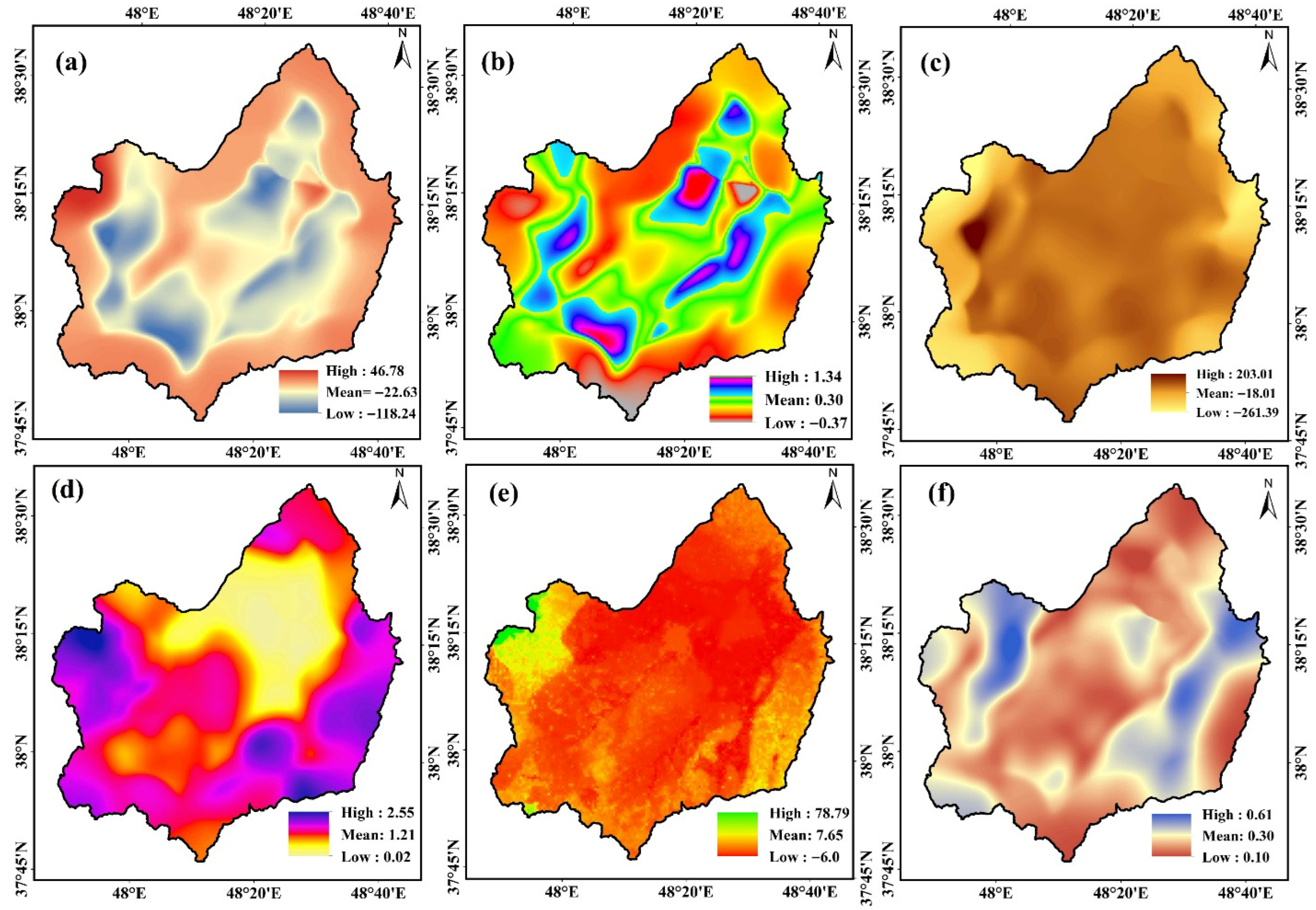
Spatial distribution of GWR statistics: (a) intercept, (b) regression coefficient (RC) of R-factor, (c) regression coefficient of K-factor, (d) regression coefficient of LS-factor, (e) regression coefficient of C-factor, and (f) Local R2.
The goodness-of-fit indices for the OLS and GWR models in the Qara-Su watershed are presented in Table 2.
According to the results in Table 2, the model with an adaptive kernel and an optimal neighborhood size of 1000 neighbors yielded a residual sum of squares of 167,951, an effective number of parameters of 9.63, a Sigma of 20.35, and an AICc of 3687.04. Compared to the OLS model with an AICc of 97,848.26 (for the 13,845-point sample), this indicates a significant improvement in local fit. The local coefficient of determination was R2 = 0.62, and the adjusted local coefficient of determination was Adjusted R2 = 0.62, indicating that approximately 62% of the local variation in erosion is explained by the R, P, LS, C, and K factors. Figure 4 shows the spatial distribution of statistics from the GWR model in the Qara-Su watershed.
To move beyond qualitative statements and provide a quantitative basis for comparing the influence of RUSLE factors, the relative importance of each driver was ranked using the mean of the absolute values of their local GWR coefficients (β). This approach summarizes the average magnitude of each factor’s effect across the watershed, a standard practice in GWR analysis [41].
As presented in Table 3, the soil erodibility (K) factor had the highest mean absolute coefficient, indicating its strong, spatially variable influence (the negative mean suggests complex local suppression effects). This was followed by the support practice (P) and topographic (LS) factors. While the cover-management (C) factor had a lower average magnitude, its spatially variable sign (frequent negative coefficients in agricultural zones, as shown in Figure 4e) confirms its localized protective role. This quantitative ranking substantiates the interpretation that LS dominates in highlands while C provides critical localized protection.
Table 3.
Mean local GWR coefficients for RUSLE factors.
The relative importance of factors was ranked by the absolute mean of local GWR coefficients (Table 3).
LS ranks high overall with strong local influence in highlands, while C exhibits protective negative coefficients in agricultural zones, aligning with mapped patterns (Figure 4).
According to the results in Figure 4, the local R2 map shows that the highest model explanatory values (up to 0.61) are concentrated in the central and southwestern parts of the watershed, where the LS and C factors have greater relative importance, while lower R2 values are observed in the northern areas. These spatial patterns clearly confirm the spatial non-stationarity of the relationships and can serve as a basis for prioritizing targeted conservation actions, such as terracing and contour farming in areas with high LS coefficients and improving vegetation cover in areas with unfavorable C coefficients. In this regard, Peng [10] in Ethiopia, showing topographic–hydrological heterogeneity, also demonstrated the superiority of GWR in mapping the local importance of factors and prioritizing conservation actions, which is supported by the local R2 results of the present study.
The analysis of the results presented in Figure 4 revealed that negative intercept values are primarily distributed in the northern and marginal areas of the watershed, indicating a lower baseline erosion rate in these regions in the absence of other factors, while positive values are observed in the central section. The local coefficient of the R-factor exhibits the least spatial variability, with its highest values concentrated in the northern areas, aligning with the higher rainfall distribution in these parts. The K-factor shows higher positive coefficients in the central and southwestern sections, reflecting the greater susceptibility of soils in these areas to erosion. Furthermore, the LS-factor has the highest relative local importance, with its highest coefficient values (up to 2.55) distributed in the southwestern mountainous areas; in contrast, the lowest values are observed in the northern section. The C-factor has a negative relationship with erosion across most of the watershed, confirming the protective effect of vegetation cover. However, in some central and downstream agricultural areas, positive values indicate intensified erosion due to suboptimal vegetation management. These results are consistent with the results of Mirchooli [9] in the Talar basin of Iran, who found GWR superior to OLS with higher R2 and lower AICc, proving the spatially non-stationary relationships between land-use changes and erosion. Similarly [7], applying GWR to USLE factors in the Nazas-Rodeo basin in Mexico, reported significant improvements in identifying the local relative importance of LS and C, which aligns with the high concentration of LS coefficients in steep areas and the variations in C observed in the present study.
Regarding the quantitative thresholds for conservation measures, and considering the direct relationship between slope and the LS factor, a threshold of LS > 5 (equivalent to a slope exceeding 25%) has been introduced in the manuscript as a criterion for prioritizing the implementation of terracing and contour farming. Based on reference values for the C factor, values higher than 0.4 indicate poor vegetation cover and the need for restoration measures (such as planting cover crops, implementing conservation agriculture, or rangeland rehabilitation). Regarding the qualitative comparison of the costs and economic benefits of conservation and restoration measures, it is noted that mechanical methods such as terracing, bank construction, and the installation of mechanical structures to control flow velocity within waterways require significant capital investment, and their implementation cost is considerably higher compared to biological methods (such as improving vegetation cover). In contrast, improving vegetation cover is less costly and can be implemented over a wider area. The necessity of using specific thresholds and considering economic conditions to translate the study’s results into operational programs is an important point that must be taken into account in watershed budgeting and investment in water and soil conservation measures.
3.4. Spatial Linkage of Results to Current Land Use and Management Recommendations
A comparative analysis of the local GWR coefficient maps with the current land use map reveals that the significant spatial variability of the coefficients, particularly for the C and LS factors, is directly linked to land use and management patterns. Adverse C coefficient values (positive or near-zero, indicating a weak protective effect of cover) are predominantly concentrated in areas of intensive dryland farming and low-density rangelands. Conversely, strong negative C coefficients (good protective effect) overlap with forests, dense rangelands, and orchards. Furthermore, the highest LS coefficient values are observed not only on steep slopes but also in areas lacking mechanical conservation practices such as terracing or contour bunding. This spatial concordance confirms that the current status of land cover and existing conservation measures play a decisive role in moderating or intensifying the inherent relationship between topographic potential (LS) and actual erosion. This result goes beyond a general acknowledgment of “land use impact” and pinpoints precise areas where improving vegetation management or implementing conservation practices could yield the highest return in reducing soil erosion.
The results of this study, particularly the local GWR coefficient maps, provide a robust spatial-analytical basis for prioritizing and targeting soil conservation measures in the Qara-Su watershed. Accordingly, the following concrete management recommendations are proposed:
In the high-elevation southwestern sub-watersheds characterized by very high LS coefficients and unfavorable C coefficients, implementing engineering-mechanical operations (e.g., terracing, stone bunds) combined with rehabilitation of native vegetation cover should be a planning priority.
In the central and downstream agricultural plains where the C coefficient indicates a weak protective effect, promoting conservation agriculture practices such as contour farming, residue management, and crop rotation is essential to improve soil cover and organic matter.
Areas with high rainfall erosivity (R) coefficients in the northern part of the watershed require runoff management and rainwater harvesting through structures like check dams and micro-catchments to dissipate the erosive energy of rainfall before concentrated runoff forms.
These place-based strategies will significantly enhance the efficiency and cost-effectiveness of soil conservation programs by focusing on the critical areas identified by the GWR model.
3.5. Limitations
A limitation is the absence of rainfall intensity data. Using monthly averages for the R-factor may not fully capture erosive energy from extreme events, which could affect the precision of erosion estimates and the related regression coefficients. A key consideration in this study is that the dependent variable (soil loss A) is derived from the product of the five RUSLE factors. Consequently, regressing A on these same factors introduces a potential circularity that could inflate goodness-of-fit metrics. However, the observed global OLS R2 of 0.50 (and the GWR R2 of 0.62) remains substantially below 1.0, indicating the models did not simply reconstruct the multiplicative equation. This is likely due to the non-linear integration of factors within RUSLE, data uncertainties, and genuine spatial non-stationarity. Therefore, while this approach limits causal inference, it remains valid for achieving the study’s primary objective: mapping the spatial non-stationarity of local factor influences to inform place-based erosion management. Future studies could complement these results with techniques like machine learning or sensitivity analysis that are not subject to the same constraint. Therefore, despite its conceptual limitation, this approach is justified for generating local coefficient maps and proposing place-based conservation strategies (e.g., terracing in high-LS zones, vegetation improvement in low-C areas. This study lacks direct quantitative validation of RUSLE estimates due to the absence of reliable long-term sediment data in the watershed. Therefore, the analysis focused on comparing OLS and GWR performance and revealing spatial patterns in factor relationships, rather than producing absolute erosion rates. The model outputs were qualitatively assessed through field visits and expert knowledge of the area, with mapped patterns (e.g., high erosion on steep southwestern slopes) aligning with field observations. Future studies with direct erosion monitoring are needed for quantitative model calibration.
4. Conclusions
The objective of this research was to compare the performance of OLS and GWR models in explaining the spatial pattern of soil erosion in the Qara-Su watershed of Ardabil Province. The study revealed that the mean annual soil erosion in this watershed is approximately 7.64 tons per hectare, classifying it within the moderate erosion category. Analysis with the global OLS model, which assumes a uniform relationship, explained about 50% of the erosion variance. However, statistical tests and the spatial pattern of residuals clearly confirmed the presence of strong spatial non-stationarity in the relationships between influencing factors. In contrast, the locally focused GWR model demonstrated far superior performance. By increasing the coefficient of determination to 62% and achieving a dramatically lower AICc, GWR proved its greater capability in modeling spatial heterogeneity. The local coefficient maps generated by GWR revealed that the importance of factors is not uniform across the watershed; the topographic (LS) factor plays the most significant role in the southwestern highlands, while the vegetation cover (C) factor exhibits a stronger protective effect in central and downstream agricultural lands, and the rainfall erosivity (R) factor is more influential in northern areas.
The results of this research have significant implications for soil resource management and conservation planning in heterogeneous watersheds. First, the clear superiority of the GWR model confirms that employing statistical methods which account for spatial heterogeneity is an unavoidable necessity for genuinely understanding erosion mechanisms and accurately identifying critical areas. Second, the locally produced factor coefficient maps provide a practical and spatially explicit foundation for prioritizing targeted conservation actions. For example, these results specify that mechanical operations like terracing should be concentrated in areas with high LS coefficients (primarily highlands), whereas in areas with unfavorable C coefficients (such as some agricultural lands), the main strategy should focus on improving vegetation management and conservation agriculture. This ‘place-based management’ approach significantly enhances the economic and operational efficiency of soil conservation plans. The results of this study align with the general direction of prior research proving the need to consider spatial variability, while objectively testing and confirming the analytical power of the GWR model in a complex mountainous–agricultural environment in northwestern Iran.
Strengths of this research include comprehensive spatial sampling (13,845 points) to capture watershed heterogeneities, the use of field and remote sensing data for accurate RUSLE factor estimation, and the provision of practical, map-based outputs for management. However, the present study has limitations that pave the way for future research. The most significant limitation is the static nature of the analysis at a specific time, which does not account for temporal changes in factors (such as fluctuations in vegetation cover or land use). Therefore, it is suggested that future research employ Spatio-Temporal Geographically Weighted Regression (GTWR) models to understand simultaneous spatial and temporal variations in erosion. Additionally, testing more advanced models like Multiscale Geographically Weighted Regression (MGWR), which also considers the varying scale of effect for each factor, could provide a more precise understanding of erosion system dynamics in this and similar watersheds.
Author Contributions
All authors contributed to the study conception and design. Material preparation, data collection and analysis were performed by authors. The first draft of the manuscript was written by N.A., F.S.N., H.K.N. and R.M. commented on previous versions of the manuscript. All authors have read and agreed to the published version of the manuscript.
Funding
The authors did not receive support from any organization for the submitted work.
Data Availability Statement
All data generated or analyzed during this study are included in this published article.
Conflicts of Interest
The authors declare that they have no competing or conflict of interests.
References
- Borrelli, P.; Ballabio, C.; Yang, J.E.; Robinson, D.A.; Panagos, P. GloSEM: High-resolution global estimates of present and future soil displacement in croplands by water erosion. Sci. Data 2022, 9, 406. [Google Scholar] [CrossRef] [Scilit]
- Panagos, P.; Borrelli, P.; Poesen, J.; Ballabio, C.; Lugato, E.; Meusburger, K.; Montanarella, L.; Alewell, C. The new assessment of soil loss by water erosion in Europe. Environ. Sci. Policy 2015, 54, 438–447. [Google Scholar] [CrossRef] [Scilit]
- Wuepper, D.; Borrelli, P.; Finger, R. Countries and the global rate of soil erosion. Nat. Sustain. 2020, 3, 51–55. [Google Scholar] [CrossRef] [Scilit]
- Borrelli, P.; Robinson, D.A.; Panagos, P.; Lugato, E.; Yang, J.E.; Alewell, C.; Ballabio, C. Land use and climate change impacts on global soil erosion by water (2015–2070). Proc. Natl. Acad. Sci. USA 2020, 117, 21994–22001. [Google Scholar] [CrossRef] [Scilit]
- Halecki, W.; Kruk, E.; Ryczek, M. Loss of topsoil and soil erosion by water in agricultural areas: A multi-criteria approach for various land use scenarios in the Western Carpathians using a SWAT model. Land Use Policy 2018, 73, 363–372. [Google Scholar] [CrossRef] [Scilit]
- Anache, J.A.A.; Flanagan, D.C.; Srivastava, A.; Wendland, E.C. Land use and climate change impacts on runoff and soil erosion at the hillslope scale in the Brazilian Cerrado. Sci. Total Environ. 2018, 622, 140–151. [Google Scholar] [CrossRef] [Scilit] [PubMed]
- Cabral-Alemán, C.; López-Santos, A.; Padilla-Martínez, J.R.; Zúñiga-Vásquez, J.M. Spatial variation of the relative importance of the soil loss drivers in a watershed of northern Mexico: A geographically weighted regression approach. Earth Sci. Inform. 2022, 15, 833–843. [Google Scholar] [CrossRef] [Scilit]
- Chicas, S.D.; Omine, K.; Ford, J.B. Identifying erosion hotspots and assessing communities’ perspectives on the drivers, underlying causes and impacts of soil erosion in Toledo’s Rio Grande Watershed: Belize. Appl. Geogr. 2016, 68, 57–67. [Google Scholar] [CrossRef] [Scilit]
- Mirchooli, F.; Mohammadi, M.; Sadeghi, S.H. Spatial modeling of relationship between soil erosion factors and land-use changes at sub-watershed scale for the Talar watershed, Iran. Nat. Hazards 2023, 116, 3703–3723. [Google Scholar] [CrossRef] [Scilit]
- Peng, Z.; Ahmad, I.; Dar, M.A.; Belete, M.; Abebe, M.K.; Fentaw, G.; Zewdu, G.S. Spatially adaptive modeling of soil erosion susceptibility using geographically weighted regression integrated with remote sensing and GIS techniques. Sci. Rep. 2025, 15, 42894. [Google Scholar] [CrossRef] [Scilit]
- Fenta, A.A.; Tsunekawa, A.; Haregeweyn, N.; Yasuda, H.; Tsubo, M.; Borrelli, P.; Panagos, P. An integrated modeling approach for estimating monthly global rainfall erosivity. Sci. Rep. 2024, 14, 8167. [Google Scholar] [CrossRef] [Scilit]
- Li, C.; Li, F.; Wu, Z.; Cheng, J. Exploring spatially varying and scale-dependent relationships between soil contamination and landscape patterns using geographically weighted regression. Appl. Geogr. 2017, 82, 101–114. [Google Scholar] [CrossRef] [Scilit]
- Zhu, C.; Zhang, X.; Zhou, M.; He, S.; Gan, M.; Yang, L.; Wang, K. Impacts of urbanization and landscape pattern on habitat quality using OLS and GWR models in Hangzhou, China. Ecol. Indic. 2020, 117, 106654. [Google Scholar] [CrossRef] [Scilit]
- Mohammed, N.H.; Abed, F.H.; Al-Khafaji, S.N. Spatial analysis of the relationship of ground slopes with water erosion using the Ordinary Least Squares (OLS) and Geographically Weighted Regression (GWR) method in ArcGIS Desktop. Uruk J. Hum. Sci. 2021, 14, 33. [Google Scholar]
- Bergsma, E.; Charman, P.; Gibbons, F.; Hurni, H.; Moldenhauer, W.C.; Panichapong, S. Terminology for Soil Erosion and Conservation: Concepts, Definitions and Multilingual List of Terms for Soil Erosion and Conservation in English, Spanish, French and German; ISSS/ITC/ISRIC: Wageningen, The Netherlands, 1996. [Google Scholar]
- Bergsma, E. Erosion intensity evaluated from micro-topographic soil erosion features, and its correlation with conservation practices, presence of fertiliser, and the erosion development between contour hedges; data of Doi Thung, northern Thailand. Sustain. Glob. Farm 2001, 666–675. [Google Scholar]
- Fotheringham, A.S.; Yang, W.; Kang, W. Multiscale geographically weighted regression (MGWR). Ann. Am. Assoc. Geogr. 2017, 107, 1247–1265. [Google Scholar] [CrossRef] [Scilit]
- Yu, S.; Wang, F.; Qu, M.; Yu, B.; Zhao, Z. The effect of land use/cover change on soil erosion change by spatial regression in Changwu County on the Loess Plateau in China. Forests 2021, 12, 1209. [Google Scholar] [CrossRef] [Scilit]
- Yao, Z.; Zhang, Y.; Xiao, P.; Zhang, L.; Wang, B.; Yang, J. Soil Erosion Process Simulation and Factor Analysis of Jihe Basin. Sustainability 2022, 14, 8114. [Google Scholar] [CrossRef] [Scilit]
- Karolinoerita, V.; Wahyudin, Y.; Ramadhani, F.; Suryanta, J.; Nahib, I. Exploring driving factors of soil erosion using a Multiscale GWR model: A case study at Central Citarum Watershed, West Java, Indonesia. IOP Conf. Ser. Earth Environ. Sci. 2023, 1266, 012084. [Google Scholar] [CrossRef] [Scilit]
- Chuenchum, P.; Xu, M.; Tang, W. Estimation of soil erosion and sediment yield in the Lancang–Mekong river using the modified revised universal soil loss equation and GIS techniques. Water 2020, 12, 135. [Google Scholar] [CrossRef] [Scilit]
- Li, C.; Yao, J.; Huang, B.; Ding, Y.; Wu, Y.; Wu, J.; Wu, M. SLEC: Soil Loss Equation Calibration Based on Spatiotemporal Non-stationarity Statistical Model using Air-ground Data. SSRN 2025. [Google Scholar] [CrossRef] [Scilit]
- Dadashi, R.; Esmali-Ouri, A.; Mostafazadeh, R.; Haji, K. Multi-criteria evaluation of the environmental carrying capacity (ECC) of Gharesou watershed in Ardabil province to optimal utilization of watershed resource. Environ. Earth Sci. 2024, 83, 131. [Google Scholar] [CrossRef] [Scilit]
- Esfandiari Darabad, F.; Mostafazadeh, R.; Nezafat Takle, B.; Pasban, A. Modeling of Suspended Sediment Yield in Ardabil Province watersheds using PCA and Multiple Regression Analysis. Irrig. Water Eng. 2022, 13, 143–162. [Google Scholar] [CrossRef]
- Moradzadeh, V.; Hazbavi, Z.; Esmali Ouri, A.; Mostafazadeh, R.; Rodrigo-Comino, J.; Zareie, S.; Fernández-Raga, M. A multifunctional conceptual framework for ecological disturbance assessment. Earth Syst. Environ. 2025, 9, 51–69. [Google Scholar] [CrossRef] [Scilit]
- Mantel, S.; Dondeyne, S.; Deckers, S. World reference base for soil resources (WRB). In Encyclopedia of Soils in the Environment, 2nd ed.; Goss, M.J., Oliver, M.A., Eds.; Elsevier: Amsterdam, The Netherlands, 2023; pp. 206–217. [Google Scholar] [CrossRef] [Scilit]
- Mostafazadeh, R.; Talebi Khiavi, H.; Esmali Ouri, A.; Asgari, E.; Golshan, M. Plot-size runoff and sediment yield affected by the type of geological formations and implications for water erosion in a semi-arid region. Model. Earth Syst. Environ. 2024, 10, 869–882. [Google Scholar] [CrossRef] [Scilit]
- Namdar, F.; Mahmoudi, S.; Esmali Ouri, A.; Pazira, E. Investigating the effect of land use changes on soil erosion using RS-GIS and AHP-Fuzzy based techniques (Case Study: Qaresu Watershed, Ardabil, Iran). Nexo Rev. Cient. 2020, 33, 525–538. [Google Scholar] [CrossRef] [Scilit]
- Mostafazadeh, R.; Talebi Khiavi, H.; Esmali-Ouri, A.; Golshan, M. Surface runoff and sediment yield response under the rainfall simulation condition controlled by soil variables of a semi-arid landscape. Environ. Dev. Sustain. 2023, 25, 12339–12356. [Google Scholar] [CrossRef] [Scilit]
- Prasannakumar, V.; Vijith, H.; Abinod, S.; Geetha, N. Estimation of soil erosion risk within a small mountainous sub-watershed in Kerala, India, using Revised Universal Soil Loss Equation (RUSLE) and geo-information technology. Geosci. Front. 2012, 3, 209–215. [Google Scholar] [CrossRef] [Scilit]
- Talebi Khiavi, H.; Mostafazadeh, R. The spatiotemporal dependencies of terrain indices with soil characteristics in a steep hillslope mountainous area. Arab. J. Geosci. 2022, 15, 937. [Google Scholar] [CrossRef] [Scilit]
- Wischmeier, W.H. A rainfall erosion index for a universal soil-loss equation. Soil Sci. Soc. Am. J. 1959, 23, 246–249. [Google Scholar] [CrossRef] [Scilit]
- Haji, K.; Khaledi Darvishan, A.; Mostafazadeh, R. Soil erosion and sediment sourcing in the Hyrcanian forests, Northern Iran: An integration approach of the G2loss model and sediment fingerprinting technique. Model. Earth Syst. Environ. 2024, 10, 1897–1914. [Google Scholar] [CrossRef] [Scilit]
- Parveen, R.; Kumar, U. Integrated approach of universal soil loss equation (USLE) and geographical information system (GIS) for soil loss risk assessment in Upper South Koel Basin, Jharkhand. J. Geogr. Inf. Syst. 2012, 4, 588–596. [Google Scholar] [CrossRef]
- Ostovari, Y.; Ghorbani-Dashtaki, S.; Bahrami, H.A.; Naderi, M.; Demattê, J.A.M.; Kerry, R. Modification of the USLE K factor for soil erodibility assessment on calcareous soils in Iran. Geomorphology 2016, 273, 385–395. [Google Scholar] [CrossRef] [Scilit]
- Zhu, X.; Liang, Y.; Tian, Z.; Wang, X. Analysis of scale-specific factors controlling soil erodibility in southeastern China using multivariate empirical mode decomposition. Catena 2021, 199, 105131. [Google Scholar] [CrossRef] [Scilit]
- Wischmeier, W.H.; Smith, D.D. Predicting rainfall erosion losses: A guide to conservation planning. In The USDA Agricultural Handbook No. 537; USDA: Beltsville, MD, USA, 1978. [Google Scholar]
- Tiruwa, D.B.; Khanal, B.R.; Lamichhane, S.; Acharya, B.S. Soil erosion estimation using geographic information system (GIS) and revised universal soil loss equation (RUSLE) in the Siwalik Hills of Nawalparasi, Nepal. J. Water Clim. Change 2021, 12, 1958–1974. [Google Scholar] [CrossRef] [Scilit]
- Stocking, M.A.; Elwell, H.A. Rainfall erosivity over Rhodesia. Trans. Inst. Br. Geogr. 1976, 1, 231–245. [Google Scholar] [CrossRef] [Scilit]
- Congalton, R.G.; Green, K. Assessing the Accuracy of Remotely Sensed Data: Principles and Practices, 3rd ed.; CRC Press: Boca Raton, FL, USA, 2019. [Google Scholar] [CrossRef] [Scilit]
- Fotheringham, A.S.; Brunsdon, C.; Charlton, M. Geographically weighted regression. In The SAGE Handbook of Spatial Analysis; Fotheringham, A.S., Rogerson, P.A., Eds.; SAGE Publications: London, UK, 2009; pp. 243–254. [Google Scholar]
- Comber, A.; Brunsdon, C.; Charlton, M.; Dong, G.; Harris, R.; Lu, B.; Lu, Y.; Murakami, D.; Nakaya, T.; Wang, Y.; et al. A route map for successful applications of geographically weighted regression. Geogr. Anal. 2023, 55, 155–178. [Google Scholar] [CrossRef] [Scilit]
- Dismuke, C.; Lindrooth, R. Ordinary least squares. In Methods and Designs for Outcomes Research; Chumney, E.C., Robinson, K.R., Eds.; American Society of Health-System Pharmacists: Bethesda, MD, USA, 2006; pp. 93–104. [Google Scholar]
- Griffith, D.A. Spatial-filtering-based contributions to a critique of geographically weighted regression (GWR). Environ. Plan A 2008, 40, 2751–2769. [Google Scholar] [CrossRef] [Scilit]
- Korkanc, S.Y.; Ozyuvaci, N.; Hizal, A. Impacts of land use conversion on soil properties and soil erodibility. J. Environ. Biol. 2008, 29, 363–370. [Google Scholar]

Disclaimer/Publisher’s Note: The statements, opinions and data contained in all publications are solely those of the individual author(s) and contributor(s) and not of MDPI and/or the editor(s). MDPI and/or the editor(s) disclaim responsibility for any injury to people or property resulting from any ideas, methods, instructions or products referred to in the content. |
© 2026 by the authors. Licensee MDPI, Basel, Switzerland. This article is an open access article distributed under the terms and conditions of the Creative Commons Attribution (CC BY) license.