Physics-Guided Data Fusion-Based Cyberattack Detection for Distributed Energy Resource Aggregators with Limited Observability

Abstract

False data injection attacks (FDIAs) pose a growing threat to distributed energy resource (DER) aggregators because a compromised aggregator can expose and affect a number of enrolled DERs. However, DER aggregators only have access to limited measurements from DERs and the systems. This makes existing FDIA detection methods ineffective in this setting due to two main limitations: (1) they are grounded in full observability of a microgrid or distribution system and therefore are incompatible with the limited observability of a DER aggregator; (2) they can only either detect anomalies or explain why a deviation occurs, but not both simultaneously. To address these limitations, we propose a physics-guided fusion-based cyberattack detection method specifically designed for DER aggregators. This approach integrates two complementary modules: a forecasting-assisted residual method for rapidly anomaly detection, and a PV-aware sensitivity-based method to diagnose and explain their underlying physical causes. A gradient boosting machine (GBM) is then leveraged to fuse these outputs, optimizing the precision–recall tradeoff. The proposed method is tested on one microgrid test system with different bus observability levels across static and gradual attack scenarios with multiple levels of attack sophistication. Across the scenarios, the proposed method achieves a 0.91–0.93 precision–recall area under the curve score (PR-AUC), demonstrating the method’s effectiveness in securing DER aggregators with partial system visibility.

1. Introduction

Distributed energy resources (DERs) and DER aggregators are changing the cybersecurity landscape of microgrids in distribution systems. DERs are small-scale generation devices, such as solar PV, battery storage, and wind turbines. There is a push to modernize the current electrical grid by increasing the amount of DER generation available [1]. DER integration in microgrids can improve resilience during outages by enabling local generation to serve critical loads when islanded from the distribution grid, but it depends on adequate DER capacity, storage, and control [2]. The variability of DERs, particularly intermittent resources such as PV, is also a constraint on the benefits during power outages. DERs and DER aggregators create a new entry point for adversaries to exploit because cybersecurity protections are not consistently implemented between legacy devices and newer Internet of Things (IoT) devices [3].

Adversaries can deploy false data injection attacks (FDIAs) to disrupt the stability of microgrids. Traditional methods to detect FDIAs utilize state estimation, which requires access to extensive bus and/or branch measurements in a microgrid or distribution system [4]. Machine learning (ML)-based methods are also evaluated under full observability assumptions [5]. All of these methods capture only a single aspect of anomalies, either how much the observed measurements deviate from their true values or which devices account for the deviations [6]. Traditional detectors, like bad-data detection and residual energy, determine an attack by the extent to which all observed measurements deviate from their forecasted or expected values. ML detectors can explain which buses deviate by isolating attacks from normal values. With all detectors, there is a tradeoff between the false alarms raised and attacks detected [7].

There are three main challenges with existing detection methods: (i) most assume full system observability, which is impractical for DER aggregators; (ii) existing methods are either physics-based or ML-based (data-driven) and therefore usually only capture one dimension of an anomaly; and (iii) balancing precision–recall in imbalanced attack datasets remains difficult. In this paper, a physics-guided data fusion-based detection method tailored to the DER aggregator setting is proposed. The central premise is that a good detector for this application must be accurate, interpretable, and deployable with only the measurements available to an aggregator.

1.1. Literature Review

In cyber–physical systems, FDIAs are becoming more complex and learn the dynamics of the system and temporal relationships between devices, which becomes a large concern for securing legacy DERs that do not inherently have cybersecurity parameters [8]. Two types of FDIAs are static and gradual, and both aim to manipulate the measurement of devices, such as voltage magnitude or power injections, to alter their operating behavior [9]. In a static FDIA, the measurements are manipulated instantaneously by an adversary-controlled perturbation (i.e., a scaling factor applied to a voltage or power measurement). In a gradual FDIA, the measurements are manipulated incrementally over a period of time until reaching the target values. Cyberattack detection mechanisms are being explored to detect FDIA before the system fails [10].

1.2. Generic Cyberattack Detection Approaches

Residual-based detection strategies compare actual values and the expected or estimated values and flag suspicious values with large residuals relative to those observed under normal operation states [11]. Residual-based detectors can be implemented in inverter-based microgrids by computing residual vectors for quantities, such as power, voltage, and current, and comparing the system states with their expected values, and the detector can recover the system states under non-attack conditions [12]. In state estimation, the threshold separating attack and normal conditions may be dynamically changed in order to accommodate for different areas within a distribution system that require greater sensitivity [13]. However, residual-based detectors can only quantify the magnitude of deviations. They are not able to pinpoint the specific buses responsible for the cyberattack.

ML-based detectors can either determine if an observed measurement deviates from a forecasted value or explain which buses contribute most to the deviation [14]. Power systems are time critical, so it is important to accurately identify an attack while minimizing false alarms. Unsupervised learning does not use training labels to determine if a value is expected or anomalous, while supervised learning requires training labels (attack versus normal) to inform its decisions. Isolation forest is an unsupervised approach that separates training data into trees and isolates anomalous data points very fast [15]. Isolation forest has been used to detect FDIAs in power systems by analyzing meter data to determine if they are bad data or valid measurements [16]. Because isolation forest is not trained on attack labels, it cannot directly optimize the tradeoff between false alarms and attack detection, making it difficult to tune the detector for imbalanced datasets. Gradient Boosting Machine (GBM) is a supervised learning model that is used for regression and classification and combines multiple trees to improve accuracy while also reducing error [17]. It can learn attack patterns during training and detect them during testing [18]. GBM can also predict bus load values and support FDIA detection by understanding the expected load forecasting for a specific time [19].

1.3. Detection Methods for DER Aggregators

A DER aggregator is an intermediary entity that coordinates multiple small-scale DERs as a single resource toward grid operators and wholesale electricity markets [20]. FERC Order No. 2222 allows DER aggregators to participate alongside traditional resources in regional electricity markets, making their secure operation a growing priority [21]. DER aggregators introduce a distinct cybersecurity challenge because a compromised aggregator can expose multiple enrolled DERs simultaneously, creating a much broader impact than the compromise of any individual device. Recent DER cybersecurity studies also indicate that detection methods tailored to the aggregator’s operational context remain largely underdeveloped [22]. More importantly, DER aggregators only observe the buses and devices enrolled in their programs, so they do not have access to the full distribution-system topology or all bus measurements [23]. This limited observability distinguishes aggregators from utility distribution operators and prevents direct application of detection methods that rely on system-wide measurements or full-network state estimation. A practical detection method must therefore be designed specifically for the aggregator’s partial-observability setting.

Cyberattack detection has also been studied in virtual power plants (VPPs), which aggregate multiple DERs to operate as a single dispatchable resource, similar in structure to a DER aggregator [24]. A non-ML approach uses a one-to-one voltage mapping that compares observed voltages against a predefined normal operation region and flags any voltage outside that boundary as an intrusion [25]. This threshold-based method quantifies the magnitude of the deviation but cannot identify which device or bus is responsible. An ML-based approach uses an unsupervised autoencoder to learn normal VPP operating patterns from unlabeled data; voltages reconstructed with large errors are flagged as anomalous [26]. While this captures complex data patterns without requiring attack labels, it cannot optimize the tradeoff between false alarms and missed attacks in imbalanced datasets. Both methods assume full system observability, making them incompatible with the partial observability constraints of a DER aggregator.

1.4. Contributions

This paper focuses on detecting static and gradual FDIAs that can occur in a microgrid within a distribution system. The main contributions of this paper are as follows:

• A forecasting-assisted, residual-energy detector (FARED) is developed for cybersecurity anomaly detection. The distribution voltage forecasting is achieved using an advanced time-series Tabular Prior-Data Fitted Network (TabPFN) foundation model with robust zero-shot and few-shot learning capabilities [27].
• A physics-based sensitivity analysis detector (SAD) is created to explain voltage deviations based on PV generation and load curve sensitivity coefficients, thereby distinguishing physically plausible deviations from suspicious ones.
• A physics-guided data fusion algorithm is developed for the aggregator setting by fusing the FARED and SAD methods using a GBM model [28].
• The proposed method is evaluated against residual energy detector, isolation forest, and GBM-based methods. The results show that the proposed approach achieves the best overall balance between attack detection and false alarms.

The remainder of this paper is organized as follows: Section 2 presents the proposed physics-guided data-fusion detection methodology. Section 3 describes the test case setup, cyberattack scenarios, and benchmark detection algorithms. Section 4 compares performance of all cyberattack detection algorithms. Section 5 presents the overall results and performance comparison. Section 6 concludes this paper and outlines future work.

2. Physics-Guided Data Fusion-Based Cyberattack Detection Methodology

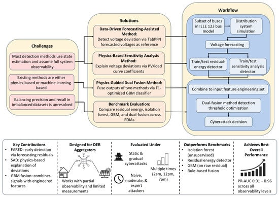
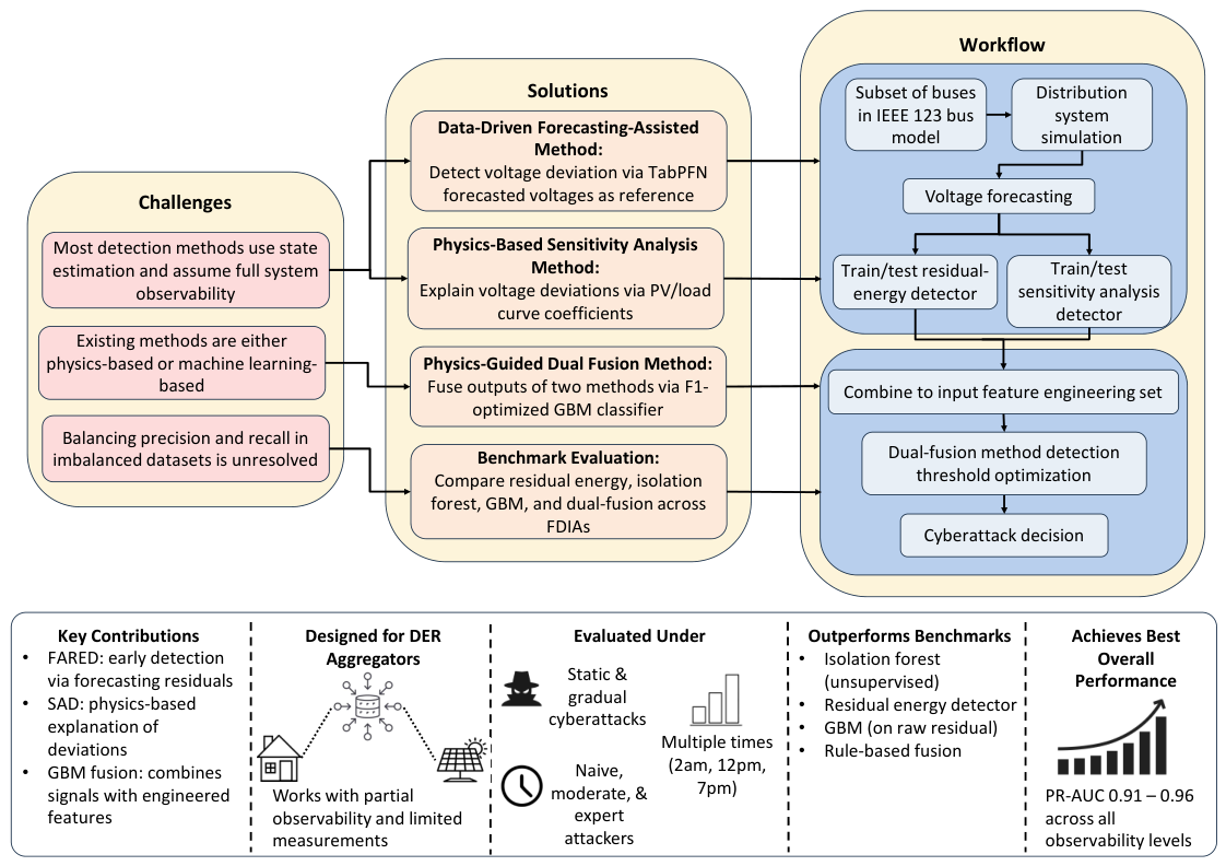
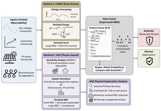
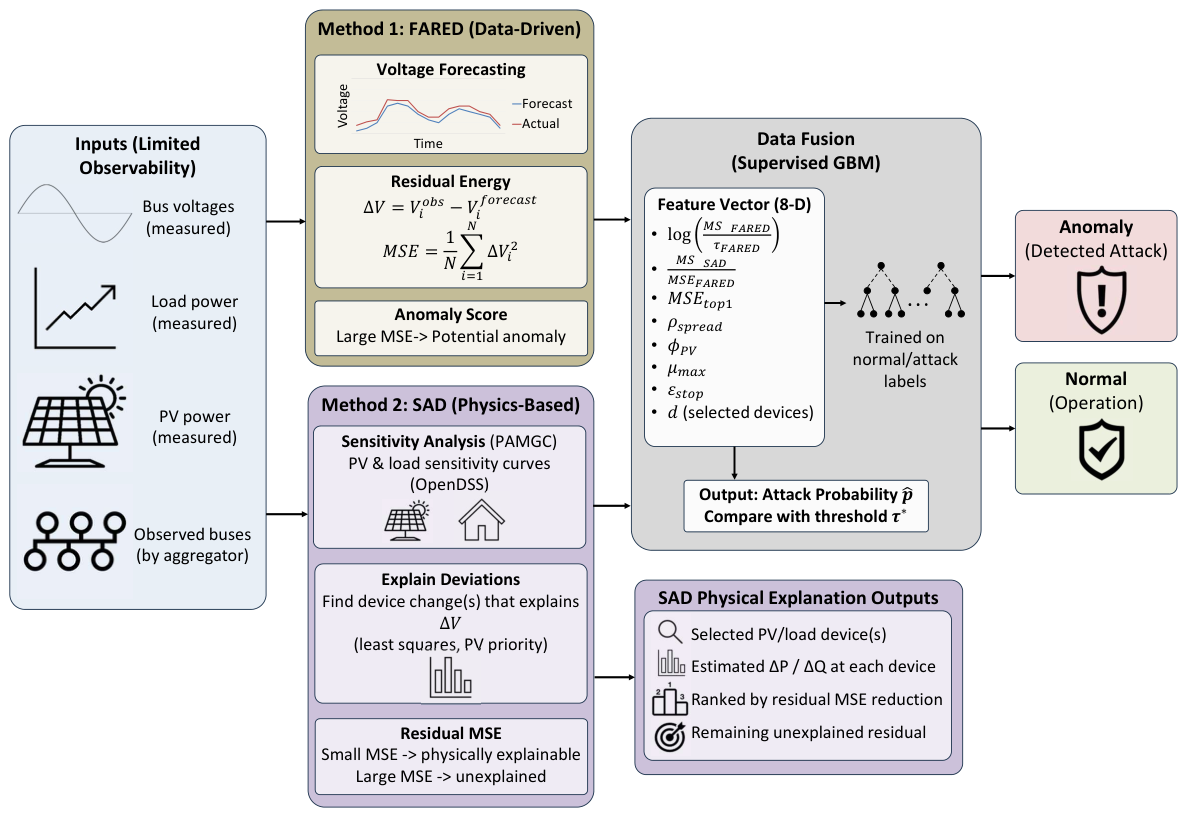
Figure 1 illustrates the proposed method and the overall workflow. The proposed detection algorithm combines the outputs of two complementary methods into a single classification. Specifically, one method quantifies the residual energy of the observed quantities, while the other explains why those deviations occur. Forecast-assisted residual energy detection (FARED) is a data-driven method that focuses on the residual of measurements collected from a subset of buses in a microgrid. In contrast, sensitivity analysis detection (SAD) is physics-based and can help explain why there is a deviation from the expected value and determine the components most likely to be under attack. Unlike conventional methods, this work does not use state estimation. It uses bus voltages and power injections from only a subset of buses in a microgrid, making it suitable for the limited observability available to a DER aggregator. The final detection method is optimized to achieve a favorable precision–recall tradeoff. The detailed structure, key equations, and key components of the proposed physics-guided, data-fusion method are shown in Figure 2.

2.1. Forecast-Assisted Residual Energy Detection

FARED operates as a residual energy detector by quantifying the extent to which observed voltages deviate from forecasted voltages. Under normal operation conditions, observed voltages should differ only slightly from the forecasted voltages because the loads and PV outputs follow predictable patterns. Large residuals indicate a potential anomaly that may be attributed to a fault, cyberattack, or unexpected disturbance, and an anomaly flag is raised when the voltage deviation exceeds a threshold learned from normal operating data during training.

Forecasting expected voltage plays a critical role in the aggregator context because DER aggregators lack full system observability and cannot use state estimation to obtain full system states. Forecasted voltages act as a semi-ground-truth reference against which observed bus voltages are compared, which enables FARED to compute residuals that capture deviations attributable to cyberattacks rather than normal load and PV variation.

Several classes of forecasting models are viable in this setting, each with distinct limitations. Classical statistical models, such as Seasonal Autoregressive Integrated Moving Average (SARIMA), capture periodic load trends well but exhibit degraded accuracy under rapid output fluctuations, making them prone to error in PV-rich microgrids where large, fast-changing voltage swings are common [29]. Recurrent neural network architectures such as long short-term memory (LSTM) can capture the non-linear voltage patterns introduced by PV generation but require large labeled training datasets to generalize effectively [30]. Both model classes also typically assume full system observability, whereas DER aggregators operate under partial observability with limited measurement access and computational resources.

TabPFN (specifically the TabPFN v2 model) is a leading foundational model for tabular data forecasting and used to forecast voltages within the microgrid because it is specifically designed for tabular data and does not require large datasets to achieve accurate predictions, demonstrating strong few-shot and even zero-shot learning capabilities [31]. Unlike traditional forecasting models, it does not require separate training and hyperparameter tuning stages to achieve good forecasting performance. The voltages forecasted by TabPFN are suitable inputs for a DER aggregator because aggregators do not inherently have access to complete knowledge of the microgrid. TabPFN also naturally supports the inclusion of exogenous covariates, such as load and PV power, within the same tabular regression framework without requiring separate preprocessing pipelines [32]. This native covariate support makes it well suited for voltage forecasting in distribution systems, where bus voltages are directly driven by device-level power injections throughout the day.

Bus voltage, load power, and PV power are input signals to the forecasting model [27]. Selective lagging strategies are used to forecast bus voltage. A 1 h short lag captures immediate temporal trends throughout a day, and a 24 h daily lag accounts for seasonality and recurring load and generation patterns. Load and PV power are exogenous features that help train the forecasting model to explain voltage changes throughout the day based on load and PV changes at the current and previous time steps. These lagging strategies and exogenous features enable the forecasting model to capture short-term transients and daily voltage trends. The model is trained on historical data and evaluated over a held-out test period.

TabPFN is deployed as a feature-engineered tabular regressor rather than a native raw-sequence model. Each sample is a single timestamp represented by the lagged feature vector, not a sliding window of raw observations. A separate model is fit per bus-phase channel via TabPFN’s in-context learning mechanism on that channel’s full six-month January–June training table, with no re-fitting at each prediction step. The fitted model is then queried independently for every July–August test timestamp on that channel. Missing covariate values are not imputed at inference time. Rows that do not have any lag or exogenous features available, such as the first day of data before daily lags can be computed, are excluded from both the training and test tables rather than filled or estimated.

2.2. Sensitivity Analysis Detection Method

SAD is introduced because a large voltage residual alone does not reveal whether the deviation arises from a cyberattack or from a legitimate physical change in operating conditions. In the DER aggregator setting, this distinction is especially important because the aggregator has only partial observability and therefore cannot rely on state estimation to interpret abnormal measurements. SAD addresses this gap by asking a physics-grounded question: can the observed voltage residual be explained by plausible changes in the loads or PV devices that the aggregator monitors?

To answer this question, SAD computes the mean squared error (MSE) between observed and forecasted voltages and then identifies the device changes that most effectively reduce that MSE. Sensitivity analysis techniques match predetermined device-curve coefficients for loads and PVs to the observed voltage residuals. If a known device change can sufficiently reduce the MSE, the deviation is treated as physically explainable and therefore more likely to be legitimate; otherwise, it is classified as anomalous.

This role makes SAD complementary to FARED. FARED is designed to be an early warning detector that is highly sensitive to deviations from forecasted behavior, but it does not determine whether those deviations are physically consistent with expected device actions. SAD provides that missing interpretability layer by evaluating whether the residual pattern can be reconstructed from legitimate device sensitivities. Consequently, FARED answers “how abnormal is this measurement pattern?”, whereas SAD answers “can this pattern be explained by plausible device behavior?” Their combination improves detection performance because the two methods capture different but complementary evidence of abnormal operation.

Sensitivity Analysis Formulation

Sensitivity analysis is conducted to match operating case studies to predetermined curve coefficients in each microgrid. The observed voltage is subtracted from the forecasted/expected voltage to determine its voltage residual, $\Delta V$. Predetermined curve coefficients are used to match the expected changes in load power and PV outputs based on the observed $\Delta V$, and the MSE is calculated to determine the closest match.

Two sensitivity analyses, Multi-Base Greedy Classifier (MBGC) and PV-Aware ordinary least squares (OLS) Solver (PVAOS), use chosen base buses to normalize the $\Delta V$ of the buses. The greedy classifier in MBGC iterates through all predefined base buses and selects the load or PV that reduces the MSE most at each step based on predetermined curve coefficients [33,34]. PVAOS extends traditional OLS regression by incorporating a PV-favored sparse selection, accounting for the smaller voltage impact of PVs relative to loads. Devices are ranked using a PV-boosted ridge regression score, and OLS is applied to the top-ranked candidates to estimate magnitudes [35,36]. Both MBGC and PVAOS normalize voltage sensitivities relative to a chosen base bus, which introduces selection bias: the choice of base bus—whether selected by largest, smallest, or average sensitivity—directly affects device identification results. An additional post-processing step is therefore required to reconcile estimates across runs with different base buses. All three techniques rely on MSE and voltage residuals to identify the best-matching device and load/PV change.

The PV-Aware Matrix Greedy Classifier (PAMGC) evaluates the system as a whole rather than linearizing values with respect to a single bus. To make the method PV-Aware, PV candidates are boosted to be comparable with loads. The design matrix is determined from the load and PV curve coefficients using L2-normalization, which reduces variance in device-selection decisions. PAMGC performs a forward selection with PV priority then solves a least-squares problem [37,38]. If the MSE of the PV hypothesis is comparable to that of the load hypothesis, the PV MSE is selected. The analysis stops when a set of devices reduces the MSE to at or below a predefined threshold or when the number of selected devices reaches the maximum allowable value. The steps and equations are shown in Algorithm 1.

Algorithm 1 PV-Aware Matrix Greedy Classifier

1: Calculate original voltage residual vector at iteration k: $$\Delta {\mathbf{V}}^{\left(k\right)}\left(x\right)={\left[\Delta V_1^{\left(k\right)}\left(x\right),\dots ,\Delta V_M^{\left(k\right)}\left(x\right)\right]}^{\top }$$ $$\Delta V_i^{\left(k\right)}=V_i^{\mathrm{observed},\left(k\right)}-V_i^{\mathrm{forecast},\left(k\right)}$$   2: Compute MSE from voltage residuals: $${\mathrm{MSE}}_{\mathrm{original}}=\frac{1}{M}{\displaystyle \sum _{i=1}^M}{(\Delta V_i^{\left(k\right)})}^2$$   3: Build predicted voltage change vector for each candidate device: $$\Delta \widehat{V}={\left[\Delta {\widehat{V}}_1\Delta {\widehat{V}}_2\cdots \Delta {\widehat{V}}_M\right]}^{\top }$$   4: Build sensitivity matrix A via centered finite difference (h > 0): $$A\approx {\displaystyle \frac{\Delta \widehat{V}(x_0+h)-\Delta \widehat{V}(x_0-h)}{2h}}$$   5: L2-normalize each column of A: $${\widehat{A}}_j=A_j/{\parallel A_j\parallel }_2$$   6: Compute ridge regression solution (PV-aware): $$u_{\mathrm{ridge}}={\left({\widehat{A}}^{\top }\widehat{A}+\lambda I\right)}^{-1}{\widehat{A}}^{\top }\Delta V^{\left(k\right)}$$   7: Rank devices by PV-boosted score: $${\mathrm{score}}_j=\left|u_{\mathrm{ridge},j}\right|\times P{V}_{\mathrm{Boost},j}$$   8: Select top-ranked devices; solve least squares and compute updated residuals: $$u_{\mathrm{OLS}}=arg\underset{u}{min}{\parallel {\widehat{A}}_{S}u-\Delta V^{\left(k\right)}\parallel }_2^2$$ $$\Delta V_{\mathrm{PV}/\mathrm{Load}}^{(k+1)}=\Delta V^{\left(k\right)}-{\widehat{A}}_S{u}_{\mathrm{OLS}}$$   9: Compute MSE for both hypotheses: $${\mathrm{MSE}}_{\mathrm{PV}/\mathrm{Load}}=\frac{1}{M}{\parallel \Delta V_{\mathrm{PV}/\mathrm{Load}}^{(k+1)}\parallel }_2^2$$ 10: Select hypothesis with lower residual: $$\Delta V=\{\begin{array}{cc}\hfill \Delta V_{\mathrm{PV}}^{(k+1)},& {\mathrm{MSE}}_{\mathrm{PV}}\le {\mathrm{PV}}_{\mathrm{gate}}·{\mathrm{MSE}}_{\mathrm{load}}\hfill \\ \hfill \Delta V_{\mathrm{load}}^{(k+1)},& \mathrm{otherwise}\hfill \end{array}$$ 11: Stop if $\mathbf{MSE}\mathbf{(}\mathbf{\Delta }{\mathit{V}}^{\mathbf{\left(}\mathit{k}\mathbf{\right)}}\mathbf{)}\mathbf{\le }\mathit{threshold}$ or k ≥ 3; else increment k and repeat.

The parameters used in Algorithm 1 are set as follows: the finite-difference step is $h=1.0$, the ridge penalty is $\lambda ={10}^{-3}$, the PV-boosted ridge score weighting factor is ${\mathrm{PV}}_{\mathrm{Boost}}=1.25$, and the PV-versus-load selection gate is ${\mathrm{PV}}_{\mathrm{gate}}=1.15$. The operating point $x_0$ used in the central-difference formula is the base-case operating point of the compiled OpenDSS model, held fixed across all test cases rather than recalibrated at each hour. $x_0$ is defined per bus-phase channel, but its value does not depend on the aggregator’s observability level. When observability is reduced, fewer bus-phase channels are included in A, but the operating point at which each remaining channel’s sensitivity is evaluated stays the same.

2.3. Anomaly Detection Using PAMGC

SAD utilizes the PAMGC to explain voltage deviations in microgrids. The goal is to find devices that can define legitimate shifts of load or PV power output throughout a day. The detection threshold is learned from training data using load and PV curve coefficients to reduce the MSE and explain changes in the system. The 97th percentile of the training residual MSEs is selected as the detection threshold. This is selected as an operating point tradeoff between sensitivity and specificity. A lower percentile increases sensitivity to true attacks but causes more false alarms, and a higher percentile reduces false alarms at the cost of missed detections. Percentile-based thresholding on training-residual distributions is common practice in FDIA and anomaly detection [39]. Legitimate voltage variations are explained by known device sensitivities and produce small residual MSEs; whereas adversarial attacks introduce power injection patterns inconsistent with expected device changes, resulting in residual MSEs that exceed the learned threshold.

2.4. Gradient Boosting Machine

GBM is a supervised learning model that takes attack and normal labels during training to learn what an attack looks like. During testing, it uses these learned attack mechanics to detect cyberattacks. The voltage residuals at each bus are found during training ($X_{train}$). The attack labels in the training data are labeled normal or attack ($y^{\left(n\right)}$). GBM takes the voltage residuals and attack labels then applies the learning parameters (100 estimators (T), learning rate of 0.1 ($\eta$), and a maximum depth of each tree of 2 ($D_{max}$)) using scikit-learn’s implementation [28]. The F1 score is used in order to optimize the precision and recall of the runs. The probability of a value being an attack (${\widehat{p}}^{\left(n\right)}$) is found then used to find the detection threshold ($\tau$), which uses the F1 score in order to find the best tradeoff between precision and recall. In the July–August test set, the probabilities of attack scores are found from the voltage residuals and compared to the learned detection threshold. If the probability score exceeds the detection threshold, then the voltages are considered anomalous.

GBM is selected as the supervised classifier for three reasons motivated by the characteristics of this dataset. First, GBM achieves strong generalization without requiring large labeled datasets, which is consistent with the limited attack-case availability in the training split. Second, its tree-based structure isolates subtle deviations effectively: anomalous voltage patterns that differ only slightly from normal behavior are separated into distinct tree branches rather than absorbed into the majority class. Third, GBM handles class imbalance through sequential boosting, which assigns increasing weight to misclassified samples at each iteration, and shallow trees further reduce overfitting by limiting each tree’s capacity to memorize training noise.

2.5. Extreme Gradient Boosting

Extreme Gradient Boosting (XGBoost) is a supervised learning model developed from GBM [40]. XGBoost has a built-in regularization term in its objective function that penalizes overly complex trees, which reduces overfitting and gives better generalization performance. It uses a second-order approximation of the loss function, using both the gradient and the curvature of the loss to weight each split, giving the model better information about whether a split correctly separates anomalous voltage patterns from normal ones. As with GBM, XGBoost handles imbalanced datasets well because each new tree is trained to correct the errors made by the previous trees. XGBoost is included as a direct comparison to GBM because it is widely used across tabular learning tasks, including settings with limited training data.

XGBoost is trained on the identical raw per-bus voltage residual feature vectors used by the standalone GBM benchmark, with the identical training/test case split, identical F1-optimal threshold calibration procedure, and identical 5-fold stratified cross-validation setup used for variance estimation. The inputs are the same as the GBM model to ensure fair testing between the detectors. XGBoost is trained with 100 estimators ($T=100$), a learning rate of 0.1 ($\eta =0.1$), and a maximum tree depth of 2 ($D_{max}=2$). The decision threshold is selected by maximizing the F1 score over the Jan–June training probability outputs, and the resulting threshold is applied to the probability-of-attack scores produced on the July–August test set.

2.6. Physics-Guided Data Fusion-Based Detection

The physics-guided data-fusion stage is designed to combine the complementary evidence produced by FARED and SAD into a single detection decision. FARED is effective at rapidly identifying deviations from forecasted behavior, whereas SAD evaluates whether those deviations are physically consistent with plausible load or PV changes. Because these two methods capture different aspects of abnormality, neither should be treated as universally dominant. The fusion stage therefore aims to reduce false positives without sacrificing true-positive detection by learning how to weigh data-driven residual evidence against physics-based explanatory evidence. Other supervised classifiers, such as logistic regression, random forests, or neural-network-based fusion, could also be used to combine the FARED and SAD outputs. GBM is adopted to keep a direct comparison with the standalone GBM benchmark used in the ablation analysis.

This subsection presents two fusion strategies. The primary method is a GBM-based fusion model, which learns the joint decision boundary from both methods and additional engineered features. A simpler conditional-rules fusion method is used as a benchmark to show the limitations of manually prioritizing one detector over the other.

2.6.1. GBM-Based Data Fusion

The GBM-based fusion method is a supervised learning approach that uses scored outputs of FARED and SAD along with engineered features to maximize the F1 score. An 8-dimensional feature vector is constructed to train the GBM fusion method (${\mathbf{X}}_{\mathrm{train}}$). The MSE values of FARED and SAD are recorded along with the flagged devices $d^{\left(n\right)}$ identified by SAD in ${\mathrm{MSE}}_{\mathrm{train}}$. From the separate training of both methods, the learned thresholds (${\tau }_{FARED},{\tau }_{SAD}$) and MSEs are found:

$${\mathrm{MSE}}_{FARED}^{\left(n\right)}={\displaystyle \frac{1}{M}}{\displaystyle \sum _{i=1}^M}{(\Delta V_i^{\left(n\right)})}^2$$

(1)

$${\mathrm{MSE}}_{SAD}^{\left(n\right)}={\displaystyle \frac{1}{M}}{\displaystyle \sum _{i=1}^M}{(\Delta V_i^{\left(n\right)}-{\widehat{V}}_i^{\left(n\right)})}^2$$

(2)

where ${\widehat{\mathbf{V}}}^{\left(n\right)}=A{u}^{\left(n\right)}$ is the SAD fitted voltage vector, $u^{\left(n\right)}$ is the selected device changes, and $d^{\left(n\right)}$ is the number of selected devices from SAD. The learned thresholds are used to log-normalize the FARED anomaly score and define the early-stop criterion for the SAD solver. The log-normalization makes the two MSE values comparable because SAD typically produces smaller MSE values by accounting for device-driven voltage deviations.

Another MSE value is found to understand the spatial awareness among the buses ${\mathrm{MSE}}_b^{\left(n\right)}$, computed over the SAD residual ${\mathbf{r}}^{\left(n\right)}=\Delta {\mathit{V}}^{\left(n\right)}-{\widehat{\mathbf{V}}}^{\left(n\right)}$:

$${\mathrm{MSE}}_b^{\left(n\right)}={\displaystyle \frac{1}{|{\mathcal{P}}_b|}}\sum _{i\in {\mathcal{P}}_b}{\left(r_i^{\left(n\right)}\right)}^2,b=1,\dots ,B$$

(3)

where ${\mathcal{P}}_b$ is the set of phase channels at bus b. This MSE value differs from FARED because it looks at individual buses and determines which bus contributes the most to the voltage deviation. This value is broken down into five additional features: the bus that carries the most weight of voltage deviations (${\mathrm{MSE}}_{\mathrm{top}1}^{\left(n\right)}$), the normalization between the most affected bus and average to determine the total voltage error (${\rho }_{\mathrm{spread}}^{\left(n\right)}$), the fraction of selected devices that are PVs (${\varphi }_{\mathrm{PV}}$), the largest device change coefficient magnitude from SAD (${\mu }_{max}$), and the unexplained anomaly flag from running SAD (${ϵ}_{\mathrm{stop}}$):

$${\mathrm{MSE}}_{\mathrm{top}1}^{\left(n\right)}=\underset{b}{max}{\mathrm{MSE}}_b^{\left(n\right)}$$

(4)

$${\rho }_{\mathrm{spread}}^{\left(n\right)}={\displaystyle \frac{{\mathrm{MSE}}_{\mathrm{top}1}^{\left(n\right)}}{{\overline{\mathrm{MSE}}}^{\left(n\right)}}}$$

(5)

$${\varphi }_{\mathrm{PV}}^{\left(n\right)}={\displaystyle \frac{\#\left\{\mathrm{PV}\mathrm{devices}\mathrm{in}{u}^{\left(n\right)}\right\}}{d^{\left(n\right)}}}$$

(6)

$${\mu }_{max}^{\left(n\right)}=\underset{k}{max}\left|u_k^{\left(n\right)}\right|$$

(7)

$${ϵ}_{\mathrm{stop}}^{\left(n\right)}=\left[{\mathrm{MSE}}_{SAD}^{\left(n\right)}>{\tau }_{SAD}\mathrm{and}{d}^{\left(n\right)}\ge K_{max}\right]$$

(8)

where $K_{max}=8$. These six spatial and device-quality features, combined with ${\mathrm{MSE}}_{FARED}^{\left(n\right)}$ and ${\mathrm{MSE}}_{SAD}^{\left(n\right)}$, form the 8-dimensional feature vector for each training sample:

$${\mathbf{x}}^{\left(n\right)}={\left[\begin{array}{c}log(1+{\mathrm{MSE}}_{FARED}^{\left(n\right)}/{\tau }_{FARED})\\ {\mathrm{MSE}}_{SAD}^{\left(n\right)}/{\mathrm{MSE}}_{FARED}^{\left(n\right)}\\ {\mathrm{MSE}}_{\mathrm{top}1}^{\left(n\right)}\\ {\rho }_{\mathrm{spread}}^{\left(n\right)}\\ {\varphi }_{\mathrm{PV}}^{\left(n\right)}\\ {\mu }_{max}^{\left(n\right)}\\ {ϵ}_{\mathrm{stop}}^{\left(n\right)}\\ d^{\left(n\right)}\end{array}\right]}^{\top }$$

(9)

SAD serves as a secondary checker because it attributes voltage deviations to specific devices. This device attribution enables the spatial features in the feature vector to isolate which buses retain unexplained voltage residuals after solving. If the voltage pattern cannot be attributed to any plausible device change, it is an indicator of an attack, and the GBM fusion method is trained to recognize these unexplained patterns.

The scikit-learn GBM formulation is used [28]. The trained GBM model ($\mathcal{M}$) has inputs of the 8-dimensional feature vector (${\mathbf{X}}_{\mathrm{train}}$), training attack and normal labels (${\mathbf{y}}_{\mathrm{train}}$), 100 decision trees (T), learning rate of 0.1 ($\eta$), and a max depth of trees of 3 ($D_{max}$):

$$\mathcal{M}=GBM\left({\mathbf{X}}_{\mathrm{train}},{\mathbf{y}}_{\mathrm{train}},T=100,\eta =0.1,D_{max}=3\right)$$

(10)

Shallow decision trees prevent overfitting by correcting residual errors from the previous tree. A 5-fold stratified cross-validation (CV) from scikit-learn is used to ensure that the attack and normal labels are proportionally represented across all folds [41]. Every sample receives an out-of-fold (OOF) probability, which is used to select a decision threshold (${\tau }^{*}$) that maximizes the F1 score between precision and recall:

$$\begin{array}{cc}\hfill {\tau }^{*}& =\underset{t\in \mathcal{T}}{arg\; max}{F}_1\left({\mathbf{y}}_{\mathrm{train}},\mathbf{1}[{\widehat{\mathbf{p}}}_{\mathrm{OOF}}\ge t]\right),\hfill \\ \hfill & \mathcal{T}=\{0.05,0.06,\dots ,0.95\}\hfill \end{array}$$

(11)

The physics-guided data fusion method (${\mathcal{M}}^{*}$) is retrained on all available training data using the best threshold. During testing, a voltage is flagged anomalous when the predicted attack probability (${\widehat{p}}_{\mathrm{test}}$) exceeds the learned threshold. Algorithm 2 describes the full process of the GBM-based data fusion method.

Algorithm 2 GBM-Based Data Fusion Detector

1: Run Methods 1 & 2 on January–June normal cases to obtain thresholds ${\tau }_{FARED},{\tau }_{SAD}$. 2: Compute ${\mathrm{MSE}}_{FARED}^{\left(n\right)}$, ${\mathrm{MSE}}_{SAD}^{\left(n\right)}$, fitted voltages ${\widehat{\mathbf{V}}}^{\left(n\right)}$, and selected devices $d^{\left(n\right)}$ from SAD (Equations (1)–(3)). 3: Compute per-bus residual MSE and spatial features ${\mathrm{MSE}}_{\mathrm{top}1}^{\left(n\right)}$, ${\rho }_{\mathrm{spread}}^{\left(n\right)}$, ${\varphi }_{\mathrm{PV}}^{\left(n\right)}$, ${\mu }_{max}^{\left(n\right)}$, ${ϵ}_{\mathrm{stop}}^{\left(n\right)}$ (Equations (4)–(8)). 4: Construct 8D feature vector ${\mathbf{x}}^{\left(n\right)}$ for each training sample (Equation (9)). 5: Train $\mathcal{M}$ via 5-fold stratified CV on Jan–June data (Equation (10)). 6: Select optimal threshold ${\tau }^{*}$ by maximizing F1 on OOF probabilities (Equation (11)). 7: Re-train final model ${\mathcal{M}}^{*}$ on all available training data. 8: For the test case, repeat Steps 2–4 to obtain ${\mathbf{x}}_{\mathrm{test}}$. 9: Compute ${\widehat{p}}_{\mathrm{test}}=P(y=1\mid {\mathbf{x}}_{\mathrm{test}},{\mathcal{M}}^{*})$; flag as anomalous if ${\widehat{p}}_{\mathrm{test}}\ge {\tau }^{*}$.

2.6.2. Rule-Based Data Fusion

For comparison, we consider a rule-based data fusion algorithm where binary rules determine whether a value is normal or anomalous based on the outputs from FARED and SAD. FARED is treated as the overruling method, and a gray zone is defined as one standard deviation from FARED’s threshold. If FARED clearly identifies a decision as normal or anomalous, the value is marked accordingly; however, if FARED’s MSE falls within the gray zone, SAD is consulted. When both methods agree that the MSE is anomalous, the case is classified as an attack. The drawback is that SAD is consulted only when FARED is uncertain, so the full information provided by SAD is not leveraged.

3. Test Cases and Scenarios

This section describes the test system, cyberattack scenarios, and benchmark detection algorithms used to evaluate the proposed method. The IEEE 123 bus system is simulated to generate training and testing data, with training spanning January–June and testing spanning July–August, at hourly resolution. Detection thresholds for all methods are learned from the training data and evaluated against normal and attack cases in the test period. This work focuses on the binary discrimination between normal operation and cyberattack cases; fault–attack differentiation is outside the scope of this study. Accordingly, any flagged measurement is treated as a cyberattack instance, as the test set comprises only normal operation and cyberattack cases.

3.1. System Model

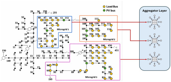
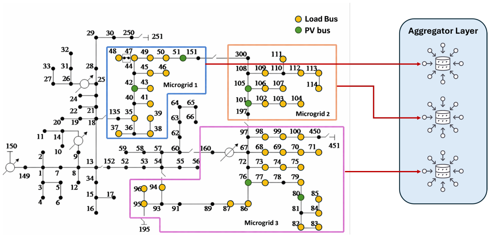
A modified IEEE 123 bus system is modeled in OpenDSS [42]. Three microgrids are defined within the model, each containing two grid-following PV inverters. All load buses are modeled as PQ loads. A normally closed switch is added between buses 47 and 48. The one-line diagram of the IEEE 123 bus system is shown in Figure 3. Bus voltage, load power, and PV power are recorded at 15 min intervals and aggregated into hourly predictions. Yearly loadshapes for the loads and PVs are drawn from the IEEE 123 bus system for OEDI SI [43]. This work is focused on microgrid 1.

3.2. Scenario Formulation

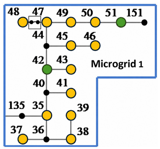
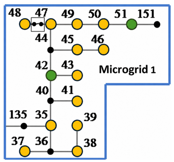
Three observability levels are evaluated to assess how the proposed method performs as the aggregator’s knowledge of microgrid 1 increases. The observed buses represent approximately 25%, 50%, and 75% of the total load buses in the microgrid. There are 12 possible load buses and 2 PV buses to be chosen, as shown in Figure 4. Both PV buses are selected in all observability levels. In the 25% observability case, load buses s35a and s37a are selected to cover more of microgrid 1 because they are on different laterals. In the 50% observability case, loads s47 and s48 are the largest loads, while s35a, s37a, s43b, and s50c are on different laterals to provide broader coverage of microgrid 1. In the 75% case, the s38b, s41c, s45a are chosen along with the rest of the 50% buses to cover more laterals within the microgrid. Bus voltages and apparent power for these loads and PVs are known and used during training and testing.

The sensitivity matrix is calculated offline using the OpenDSS model; however, an aggregator does not have full knowledge of the system. In all cases, the physics does not change. The aggregator has access only to the buses enrolled at each observability level, and each detector uses only the pre-calibrated relationships corresponding to its observed bus-phase channels.

The same reasoning applies to the FARED forecasting model. TabPFN is trained once, offline, using full-microgrid load and PV aggregates as exogenous covariates, and the same trained per-channel models are reused across all three observability levels. Reducing observability changes only which bus-phase voltage residuals are compared against the forecast at deployment, not what the forecasting model itself was trained on.

Within the January–June training data, 24 normal cases are saved per day; 27 days are chosen to apply cyberattacks, yielding a 75%/25% normal/attack split for supervised learning models. In the July–August testing data, all days include 24 normal cases, and 10 days have cyberattacks applied. Attacks are applied at three sophistication levels (naive, moderate, expert) and two types (static and gradual), tested at 2:00 a.m. (no solar), 12:00 p.m. (maximum PV generation), and 7:00 p.m. (maximum load, no solar). In the attack cases, the normally closed switch between buses 47 and 48 is open. The adversary aims to manipulate known bus voltages to make the open switch appear closed.

Naive attacks manipulate a single bus; moderate attacks manipulate half the known buses; expert attacks change all known bus voltages.

Table 1. Attacked buses by observability level.

Attack Sophistication	Observability (%)	Bus(es)
Naive	25	35
	50	35
	75	35, 37, 42, 51
Moderate	25	35, 37
	50	35, 37, 42, 43
	75	35, 37, 38, 41, 42
Expert	25	35, 37, 42, 51
	50	35, 37, 42, 43, 47, 48, 50, 51
	75	35, 37, 38, 41, 42, 43, 45, 47, 48, 50, 51

summarizes the buses attacked at each sophistication level. Static attacks immediately manipulate voltages, while gradual attacks take multiple time steps to reach the final manipulated values.

3.3. FDIA Threat Model and Mathematical Formulation

The FDIA compromises the communication channel between enrolled DER devices and the DER aggregator. It is consistent with the classical FDIA formulation by injecting malicious vector measurements into the reported measurements to the operator. The adversary does not alter the physical state of the system, but it corrupts the observed voltage measurements. The attack is constructed directly on the residuals relative to the TabPFN forecast. Static attacks apply a fixed masking strength the instant the switch opens, while gradual attacks ramp a time-varying masking fraction from 0.6 to 1.0 across five 15 min steps The same underlying mechanism unfolds instantaneously in one case and incrementally in the other.

${\mathcal{B}}_{\mathrm{obs}}$ denotes the set of bus-phase channels observed by the DER aggregator at a given observability level (25%, 50%, or 75%). $\mathcal{D}=(d_1,d_2,\dots ,d_N)$ is a fixed, ordered list of candidate target channels within ${\mathcal{B}}_{\mathrm{obs}}$. Attacker sophistication is modeled as the number of channels the attacker has compromised, taken as an ordered prefix of $\mathcal{D}$, defining the attack space evaluated as shown in Equation (12). ${\alpha }_i$ is the injected bias strength on channel i and ${\epsilon }_i\left(t\right)$ is bounded measurement noise.

${\mathcal{C}}_{\mathrm{soph}}\subseteq \mathcal{D}$ denotes the specific set of compromised channels at a given sophistication level, with $c_{\mathrm{soph}}=\left|{\mathcal{C}}_{\mathrm{soph}}\right|$ the corresponding channel count. ${\mathcal{C}}_{\mathrm{naive}}$, ${\mathcal{C}}_{\mathrm{moderate}}$, and ${\mathcal{C}}_{\mathrm{expert}}$ correspond to the bus sets listed in Table 1 for each sophistication level, and $\mathcal{A}$ denotes the resulting attack space.

$$\mathcal{A}=\left\{\left({\mathcal{C}}_{\mathrm{soph}},\left\{{\alpha }_i\right\},\left\{{\epsilon }_i\left(t\right)\right\}\right):{\mathcal{C}}_{\mathrm{soph}}=\{d_1,\dots ,d_{c_{\mathrm{soph}}}\},{\mathcal{C}}_{\mathrm{naive}}\subset {\mathcal{C}}_{\mathrm{moderate}}\subset {\mathcal{C}}_{\mathrm{expert}}\subseteq {\mathcal{B}}_{\mathrm{obs}}\right\}$$

(12)

3.3.1. Static FDIA

$V_i^{\mathrm{true}}\left(t\right)$ denotes the true, attack-free voltage at channel i with the switch open. $V_i^{\mathrm{forecast}}\left(t\right)$ is the expected voltage found from TabPFN forecasting. The physical residual is defined in Equation (13).

$${\delta }_i\left(t\right)=V_i^{\mathrm{true}}\left(t\right)-V_i^{\mathrm{forecast}}\left(t\right)$$

(13)

For compromised channels $i\in {\mathcal{C}}_{\mathrm{soph}}$, the attacker injects an additive perturbation designed to mask a fraction ${\alpha }_i$ of this residual. It changes per sophistication level with bounded noise ${\epsilon }_i\left(t\right)$, so that the value reported to the aggregator is given in Equation (14).

$$\begin{array}{cc}\hfill V_i^{\mathrm{observed}}\left(t\right)& =\left\{\begin{array}{cc}{V}_i^{\mathrm{true}}\left(t\right)-{\alpha }_i{\delta }_i\left(t\right)+{\epsilon }_i\left(t\right),\hfill & i\in {\mathcal{C}}_{\mathrm{soph}},\hfill \\ V_i^{\mathrm{true}}\left(t\right),\hfill & \mathrm{otherwise},\hfill \end{array}\right.\hfill \\ \hfill {\alpha }_i& \sim \mathcal{U}\left({\alpha }_{min}^{\mathrm{soph}},{\alpha }_{max}^{\mathrm{soph}}\right),{\epsilon }_i\left(t\right)\sim \mathcal{N}(0,{\sigma }_{\mathrm{soph}}^2)\hfill \end{array}$$

(14)

For static attacks, the masking-fraction bounds and noise standard deviation vary by sophistication level: $({\alpha }_{min}^{\mathrm{soph}},{\alpha }_{max}^{\mathrm{soph}})=(0.6,0.9)$ for naive, $(0.4,0.7)$ for moderate, and $(0.2,0.4)$ for expert attacks, with corresponding noise standard deviations ${\sigma }_{\mathrm{soph}}=0.3$, $0.8$, and $1.2$ V, respectively.

The observed residual seen by FARED and SAD is Equation (15). The attack masks a fraction ${\alpha }_i$ of the true anomaly, leaving $(1-{\alpha }_i)$ of the residual exposed to the detector plus injected noise.

$$\Delta V_i\left(t\right)=V_i^{\mathrm{observed}}\left(t\right)-V_i^{\mathrm{forecast}}\left(t\right)=(1-{\alpha }_i){\delta }_i\left(t\right)+{\epsilon }_i\left(t\right)$$

(15)

To model an adversary aware of the residual-energy detector’s operating threshold ${\tau }_{FARED}$, static attacks are additionally subject to a global energy budget over the M observed channels, shown in Equation (16). It is enforced by iteratively rescaling the attacked residuals by $s=min\left(1,\sqrt{{\tau }_{\mathrm{stealth}}/\mathrm{MSE}}\right)$ until the constraint is met, representing an optimization-aware adversary who bounds total injected energy below the detector’s learned alarm threshold.

$${\displaystyle \frac{1}{M}}{\displaystyle \sum _{i=1}^M}\Delta V_i{\left(t\right)}^2\le {\tau }_{\mathrm{stealth}},{\tau }_{\mathrm{stealth}}<{\tau }_{FARED}$$

(16)

3.3.2. Gradual FDIA

Gradual attacks replace the constant bias ${\alpha }_i$ with a time-varying masking fraction $\rho \left(t\right)$ that increases monotonically over five 15 min steps within the attack hour, indexed $t=0,1,2,3,4$ (zero-indexed, so $t=4$ is the fifth and final step), as shown in Equations (17) and (18). The masking fraction starts at 0.6 at attack onset and rises to full masking, so the ramp schedule bounds the exposed residual throughout the attack window. This achieves a stealth effect implicitly rather than through the explicit energy-budget rescaling used for static attacks.

$$\rho \left(t\right)={\rho }_0+({\rho }_4-{\rho }_0){\displaystyle \frac{t}{4}},{\rho }_0=0.6,{\rho }_4=1.0$$

(17)

$$V_i^{\mathrm{observed}}\left(t\right)=V_i^{\mathrm{true}}\left(t\right)+\rho \left(t\right)\left[V_i^{\mathrm{forecast}}\left(t\right)-V_i^{\mathrm{true}}\left(t\right)\right]+{\epsilon }_i\left(t\right),i\in {\mathcal{C}}_{\mathrm{soph}}$$

(18)

The reported residual converges toward the noise floor as $t\to 4$, as shown in Equation (19), modeling an attacker who deliberately mimics a gradual, physically plausible transition rather than an abrupt step change.

$$\Delta V_i\left(t\right)=\left(1-\rho \left(t\right)\right){\delta }_i\left(t\right)+{\epsilon }_i\left(t\right)$$

(19)

3.4. Benchmark Voltage Residual Detection

Four benchmark voltage residual detection methods are evaluated against the proposed method. The traditional method is the voltage residual energy detector, which flags deviations between observed and forecasted voltages that exceed a learned threshold. Three ML-based approaches are also evaluated. The isolation forest detection algorithm is an unsupervised learning approach that does not require attack labels, implemented using default scikit-learn parameters [44]. Anomalies are identified by their tendency to be isolated with fewer trees than normal observations. GBM and XGBoost are supervised learning-based approaches that require attack labels during training. They build sequential trees to correct errors of previous trees to classify voltage residuals as normal or anomalous.

The standalone GBM and XGBoost benchmarks operate directly on per-bus voltage residuals, using raw deviation magnitudes as their input feature set. Standalone GBM also serves as the ablation baseline for the proposed GBM fusion model. The fusion model operates on the 8-dimensional physics-guided feature vector derived from both FARED and SAD outputs. The performance gap between the two configurations therefore isolates the contribution of physics-guided feature engineering over raw residual inputs.

4. Dual-Method Fusion Detection Results

The proposed detection algorithms combine the outputs of FARED and SAD methods to obtain the final detection decision. Two fusion methods are compared: one uses binary rules to combine outputs, and the other uses feature engineering and GBM.

4.1. Voltage Forecasting Results for FARED

Three metrics are used to evaluate forecasting accuracy: mean absolute error (MAE), root mean squared error (RMSE), and mean absolute percentage error (MAPE) [45]. MAE reports the average magnitude of the forecast error in volts, treating all deviations equally regardless of size. RMSE squares each voltage error before averaging, so it penalizes large deviations more heavily than MAE. MAPE expresses the error as a percentage of the true voltage magnitude, which allows error to be compared on a common scale independent of the nominal voltage at each bus. For all three metrics, lower values indicate less variation between the forecasted and observed voltage, signaling a more accurate forecast.

Table 2. Average voltage forecasting error by observability level, TabPFN vs. SARIMA.

Observability (%)	Algorithm	Avg. MAE (V)	Avg. RMSE (V)	Avg. MAPE (%)
25	TabPFN	0.158	0.391	0.0065
	SARIMA	0.204	0.556	0.0084
50	TabPFN	0.157	0.390	0.0065
	SARIMA	0.203	0.554	0.0083
75	TabPFN	0.157	0.389	0.0064
	SARIMA	0.202	0.551	0.0083

Bold values indicate the forecasting model (TabPFN) selected for use in FARED in the final proposed method, based on its consistently lower error across all observability levels.

summarizes hour-ahead voltage forecasting accuracy across all bus-phase channels at each observability level and compares TabPFN against SARIMA. The chosen lagging strategies for TabPFN capture seasonal voltage trends, and the exogenous load and PV features explain how device powers affect voltages throughout the day. SARIMA has a univariate use, so exogenous covariates are not included. Both produce accurate forecasts; however, TabPFN has better average MAE, RMSE, and MAPE for the test set. The introduction of specific load and PV variables helps TabPFN learn the training forecasting curves from January to June and apply it to a July–August testing set. SARIMA’s seasonal autoregressive term relies on the assumption that daily patterns repeat closely from one day to the next. This assumption is more reliable in seasons with consistent weather, as in the July–August period evaluated, than in seasons with more variable day-to-day conditions.

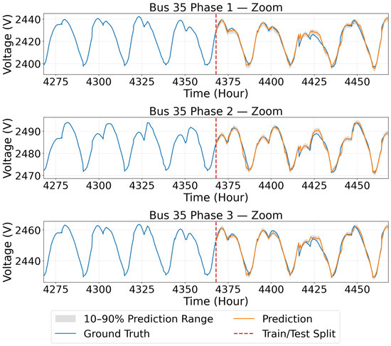
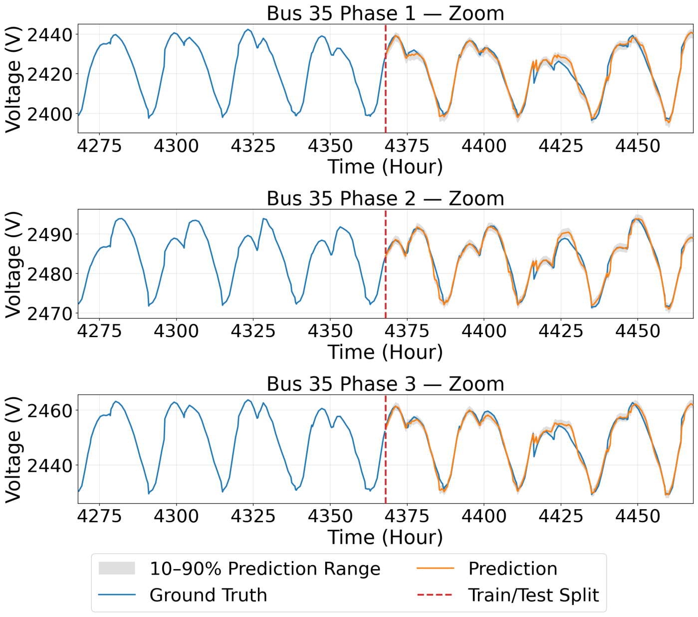
For TabPFN, the forecasted voltages follow the ground truth closely across all Bus 35 phases in Figure 5. Since the forecasting model is trained exclusively on normal operating data, attack-manipulated voltages manifest as large residuals that exceed the learned threshold and are flagged as anomalous, while small residuals reflect typical intra-day voltage variation.

4.2. SAD Data Collection and OpenDSS

The IEEE 123-bus system is simulated in OpenDSS to characterize how load and PV changes affect bus voltages. The active and reactive power of all loads and the PVs’ kVA are individually varied by ±1, 5, 10, 15, 20, 30, 40, 50 percent, and the resulting voltage change measurements $\Delta V$ are stored and separated by microgrid. Curve coefficients are determined from the $\Delta V$s: loads use a linear equation $ax+b$, while PVs use a piecewise equation to capture non-linear voltage behavior across different operating ranges, with breakpoints determined empirically from the simulation data. For PV changes, a three-segment piecewise linear equation with empirically determined breakpoints is used to capture non-linear voltage behavior across low, mid, and high operating ranges.

4.3. SAD Sensitivity Analysis Results

PAMGC demonstrates clear advantages over MBGC and PVAOS, as shown in

Table 3. Comparison of sensitivity analysis techniques.

Case	Method	Detection of Buses (%)	Buses Detected	Power Difference	Time (s)
MG1 s51a: 32 kvar s39b: 22 kvar	MBGC	100	s51a	$-4.36$	3.3
			s39b	$-0.26$
	PVAOS	100	s51a	$0.11$	0.48
			s39b	$-0.02$
	PAMGC	100	s51a	0.12	0.43
			s39b	0.01
MG2 s106b: 8 kW s111a: 14 kW	MBGC	50	s111a	1.38	2.71
			s112a	4.18
	PVAOS	100	s106b	7.45	0.3
			s112a	9.66
	PAMGC	100	s106b	6.46	0.07
			s112a	8.15
MG3 PV80: 17 kVA	MBGC	100	PV80	−2.12	4.01
	PVAOS	100	PV80	−1.57	0.8
	PAMGC	100	PV80	−2.00	0.53

Bold values indicate the sensitivity analysis model (PAMGC) selected for use in SAD in the final proposed method, based on its accuracy of detecting correct buses and fast execution time.

. It correctly identifies the active devices across all test cases, while MBGC fails in MG2 and MG3. Compared to PVAOS, PAMGC achieves consistently lower execution time and eliminates base-bus selection bias, making results reproducible without parameter tuning. Although power differences remain non-negligible in MG2, PAMGC produces the closest estimates to the true setpoints across all microgrids. Therefore, PAMGC is selected as the SAD cyberattack detection module for our proposed data fusion method.

5. Results and Performance Comparison

All detection algorithms are trained on data from January–June and tested on all days in July–August for normal operation cases and ten days with cyberattack cases. There are 1488 normal operating cases, 90 static attacks (3 sophistication levels at 3 time periods), and 450 gradual attacks (3 sophistication levels across 5 time steps at 3 time periods) within the test set.

Seven cyberattack detectors are evaluated in this work. Three ML-based benchmarks are included: isolation forest, GBM, and XGBoost. FARED, which quantifies the magnitude of voltage deviations from forecasted behavior, and SAD, which provides physics-guided attribution of those deviations to specific devices, are also tested as standalone detectors. This establishes each module’s individual contribution and characterizes how fusing their outputs improves overall performance. Two fusion configurations, rule-based and GBM-based, are then compared to quantify the benefit of combining complementary evidence.

The performance metrics used to compare the detection algorithms are accuracy, precision, recall, F1 scores, and PR-AUC and are derived from true positives (TP), true negatives (TN), false positives (FP), and false negatives (FN). A TP is the number of attacks that are correctly identified as an attack in the dataset. TN is the number of normal cases correctly identified as normal operation. A FP, also known as a false alarm, is the number of normal cases in the dataset that are incorrectly flagged as an attack. A FN, also called a miss, is the number of real attacks that go undetected and seen as normal operation in the dataset. The test set contains a maximum of 540 true positives and 1488 true negatives.

Accuracy is the fraction of all cases classified correctly:

$$Accuracy={\displaystyle \frac{TP+TN}{TP+FP+TN+FN}}$$

(20)

Precision measures the fraction of flagged cases that are true attacks:

$$Precision={\displaystyle \frac{TP}{TP+FP}}$$

(21)

Recall determines how many true attacks are detected:

$$Recall={\displaystyle \frac{TP}{TP+FN}}$$

(22)

The F1 score is the harmonic mean of precision and recall and captures large imbalances between the two:

$$F1=2·{\displaystyle \frac{Precision·Recall}{Precision+Recall}}$$

(23)

PR-AUC summarizes the precision–recall tradeoff across all decision thresholds and is particularly informative for imbalanced datasets:

$$\mathrm{PR}\text{-}\mathrm{AUC}\approx {\displaystyle \sum _{i=1}^n}Precisio{n}_i·(Recal{l}_i-Recal{l}_{i-1})$$

(24)

Table 4. Overall confusion matrix and performance metrics for all algorithms.

Observability (%)	Algorithm	TP	FP	TN	FN	Acc. (%)	Prec. (%)	Recall (%)	F1	PR-AUC
25	Isolation Forest	503	404	1084	37	78.25	55.46	93.15	0.70	0.74
	GBM	525	467	1021	15	76.23	52.92	97.22	0.69	0.87
	XGBoost	519	481	1007	21	75.25	51.90	96.11	0.67	0.90
	FARED	505	541	947	35	71.60	48.28	93.52	0.64	0.92
	SAD	476	483	1005	64	73.03	49.64	88.15	0.64	0.89
	Conditional Rule	504	485	1003	36	74.31	50.96	93.33	0.66	N/A
	GBM Fusion	522	465	1023	18	76.18	52.89	96.67	0.68	0.91
50	Isolation Forest	505	398	1090	35	78.65	55.92	93.52	0.70	0.74
	GBM	528	359	1129	12	81.71	59.53	97.78	0.74	0.87
	XGBoost	526	350	1138	14	82.05	60.05	97.41	0.74	0.92
	FARED	509	523	965	31	72.68	49.32	94.26	0.65	0.93
	SAD	490	481	1007	50	73.82	50.46	90.74	0.65	0.91
	Conditional Rule	506	471	1017	34	75.10	51.79	93.70	0.67	N/A
	GBM Fusion	526	340	1148	14	82.54	60.74	97.41	0.75	0.93
75	Isolation Forest	507	402	1086	33	78.55	55.78	93.89	0.70	0.78
	GBM	516	345	1143	24	81.80	59.93	95.56	0.74	0.86
	XGBoost	517	352	1136	23	81.51	59.49	95.74	0.73	0.91
	FARED	509	524	964	31	72.63	49.27	94.26	0.65	0.93
	SAD	490	482	1006	50	73.77	50.41	90.74	0.65	0.91
	Conditional Rule	506	473	1015	34	75.00	51.69	93.70	0.67	N/A
	GBM Fusion	534	345	1143	6	82.69	60.75	98.89	0.75	0.91

Bold values indicate the developed FDIA fusion method.

presents the overall confusion matrix and performance metrics across 2028 test cases. The proposed GBM fusion achieves the best results overall across all observability levels. In 25% observability, it achieves a 76.18% accuracy, 0.68 F1, and 0.91 PR-AUC. In 50% observability, it achieves an 82.54% accuracy, 0.75 F1, and 0.93 PR-AUC. In 75% observability, it achieves a 82.69% accuracy, 0.75 F1, and 0.91 PR-AUC. This reflects strong detection capability with different sets of observability levels. The unsupervised methods—isolation forest, FARED, SAD, and conditional rules—achieve high recall (87–93%) but produce more false alarms than the supervised methods, reducing their precision and F1. Conditional rule fusion does not produce a PR-AUC because its binary outputs yield no continuous scoring curve. The supervised GBM and XGBoost algorithms outperform all unsupervised methods, confirming that attack labels during training improve discrimination between normal and attacked voltages. Despite XGBoost’s more sophisticated regularized, second-order boosting formulation, GBM and XGBoost perform comparably at the calibrated decision threshold on F1 score and expert-level attack detection. This indicates that GBM’s simpler formulation is not a performance liability relative to XGBoost. The addition of physics-guided engineering features allows GBM Fusion to outperform both raw-residual boosting benchmarks.

The largest performance gain occurs between 25% and 50% observability, since the 50% bus set adds the two largest loads (s47, s48) along with buses on previously uncovered laterals of microgrid 1. Beyond 50%, the additional buses in the 75% case largely fall on laterals already represented. Coverage of the microgrid’s major current paths is the key driver of detection performance.

From an operational standpoint, the false-alarm rates observed here (23–31% across observability levels) impose a burden on aggregator operators. Flagged cases consume operator time and, if sustained, can lead to alert fatigue, which is a risk in security operations where high false-positive rates cause operators to deprioritize or ignore alerts over time [46]. A missed attack, FN, can allow a compromised aggregator to affect multiple enrolled DERs simultaneously, so the cost between a missed attack and a false alarm favors prioritizing recall shown in the F1 optimization. The SAD component’s device-level attribution is intended to partially offset this operational cost by presenting operators with specific device(s) implicated in the residual, which can accelerate operator triage relative to a bare anomaly flag. This recall bias is addressed entirely through the decision-threshold stage; the GBM models are trained with scikit-learn’s default equal sample weighting and do not use class-weighting during model fitting. An alternative approach would be to upweight attack-class samples during training itself, which could produce better-calibrated probability outputs and potentially reduce reliance on aggressive threshold tuning.

5.1. Performance During Normal Operation

Table 5. Normal cases confusion matrix and performance metrics.

Algorithm	25% Observability		50% Observability		75% Observability
	FP	TN	FP	TN	FP	TN
Isolation Forest	404	1084	398	1090	402	1086
GBM	467	1021	359	1129	345	1143
XGBoost	481	1007	350	1138	352	1136
FARED	541	947	523	965	524	964
SAD	483	1005	481	1007	482	1006
Conditional Rule	485	1003	471	1017	473	1015
GBM Fusion	465	1023	340	1148	345	1143

Bold values indicate the developed FDIA fusion method.

shows FPs and TNs across the 1488 normal operating hours. FARED produces the most false alarms because it cannot distinguish near-threshold voltage deviations as attack or normal behavior. Conditional rule fusion reduces false alarms by consulting SAD in the gray zone; isolation forest reduces them further through clustering and has the least amount in the 25% observability case. GBM fusion achieves the fewest FPs in the 50% and 75% cases by combining both FARED and SAD methods’ outputs with additional engineered features.

5.2. Performance Under Cyberattack Conditions

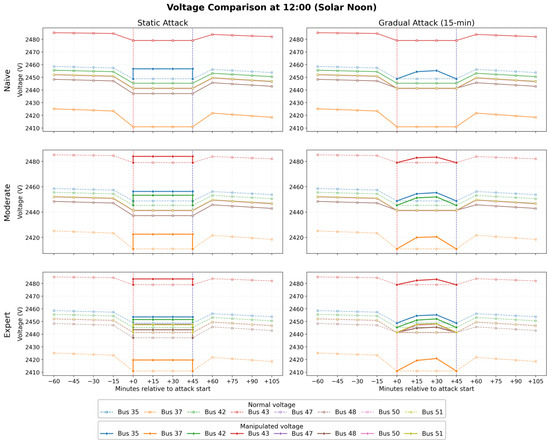
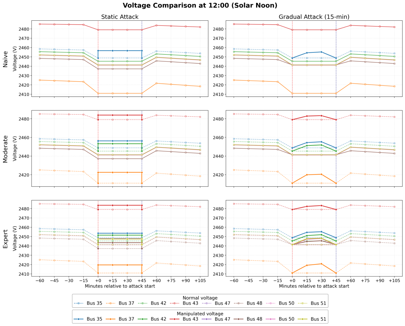
A total of 90 static and 450 gradual attack cases were evaluated. In static attacks, voltage manipulation is injected instantaneously at full magnitude rather than escalating over time. In static attacks, the injected voltage offset is applied instantaneously and held constant, so the voltage residuals remain stable throughout the attack window. Gradual attacks change output voltages incrementally across five 15 min time steps to reach the final desired voltage value. In gradual attacks, the injected voltage increases incrementally to mimic expected system behavior, causing residuals to grow over successive time steps. This makes gradual attacks more difficult to detect, particularly at early time steps where the injected perturbation is still small. All detection algorithms achieved a perfect 100% detection rate across all naive and moderate attack cases. Figure 6 shows how voltages are affected in expert-level static and gradual attacks. The same patterns are shown in all observability levels and time stamps. In static attacks, the attack looks like a step function that injects the same voltage throughout the attack period. In gradual attacks, the attacks gradually reach the values to make it look like a known behavior.

Table 6. Expert-level attack detection.

Algorithm	25% Observability				50% Observability				75% Observability
	Static		Gradual		Static		Gradual		Static		Gradual
	TP	FN	TP	FN	TP	FN	TP	FN	TP	FN	TP	FN
Isolation Forest	30	0	117	33	30	0	115	35	30	0	117	33
GBM	30	0	135	15	30	0	138	12	30	0	126	24
XGBoost	30	0	129	21	30	0	136	14	30	0	127	23
FARED	30	0	118	32	30	0	119	31	30	0	119	31
SAD	26	4	97	53	30	0	100	50	27	3	103	47
Conditional Rule	30	0	117	33	30	0	116	34	30	0	116	34
GBM Fusion	30	0	132	18	30	0	136	14	30	0	144	6

Bold values indicate the developed FDIA fusion method.

shows the TPs and FNs for expert-level attacks under both attack types. Expert attacks are the hardest to detect because they manipulate all known bus voltages to mimic normal behavior.

All algorithms except SAD in the 75% observability case achieve perfect detection against expert static attacks. SAD explains voltage deviations by fitting them to known sensitivity curves, so expert attacks that adjust all known buses can make the observed voltages appear consistent with expected device behavior. GBM fusion does not produce different detection sensitivities between static and gradual attacks.

Gradual attack cases represent the most challenging detection scenario evaluated in this study. The attacker’s goal is to make the open switch appear closed over a period of time. GBM fusion achieves the best overall detection rate, demonstrating that combining the outputs of FARED and SAD with additional feature engineering improves detection of sophisticated attacks.

DER aggregators have strict latency requirements that data transmission must follow. Automatic generation control (AGC) sends signals to the aggregator at a 4 s interval [47]. IEEE 2030.5 requires forward control updates to a control center every 1–5 min [48]. The coordination within an aggregator and grid are updated every 15–60 min [49]. The proposed GBM fusion achieves a median end-to-end inference latency of 443 ms and a 99th-percentile latency of 2.8 s, both within the 4 s scan cycle required by AGC. Detection is therefore feasible within a single control interval, including for expert-level attacks that require more device selections in the SAD solver.

6. Conclusions

This paper proposes a physics-guided data-fusion method for FDIA detection in DER aggregators operating with limited system information. The method combines FARED, which quantifies voltage deviations from expected behavior, with SAD, which explains those deviations using PV and load sensitivity information. By fusing these complementary signals within a GBM-based detector, the proposed approach addresses a key limitation of existing methods: most can either quantify abnormality or explain its source but not do both effectively under limited observability.

The proposed method was evaluated against benchmark detectors under static and gradual attack scenarios with naive, moderate, and expert attacker sophistication. Across all cases, our method achieved the best overall performance in all observability cases, with a PR-AUC ranging from 0.91 to 0.93, indicating a strong balance between cyberattack detection and false-alarm reduction. These results demonstrate that combining data-driven residual features with physics-based explanatory features improves cyberattack detection beyond methods that rely on raw voltage deviations alone.

There are three limitations of this work to be considered in future work. The first limitation of this work is that it does not explicitly distinguish anomalies caused by physical disturbances from those caused by cyberattacks. Extending fault–attack discrimination to the DER aggregator setting remains an important direction for future research. Relatedly, detection performance is directly tied to the accuracy of the underlying voltage forecast. Improved forecast accuracy under rapidly changing irradiance, load uncertainty, or DER operational changes would further sharpen the residual signal available to FARED and improve detection. Recent work has begun exploring digital twins to support more robust forecasting under these conditions as DER penetration increases [50]. The second limitation is that the full detection pipeline is validated on a single microgrid across observability levels. The SAD sensitivity-analysis component was evaluated for device-identification accuracy across all three microgrids, with consistent performance, but this does not substitute for validating detection accuracy, precision, and recall across differing topologies and observability levels. The GBM fusion detector should be tested on different systems that include more DERs and other topologies. The third limitation is that the works only look at PVs for DER integration. This work is not dependent on PVs, as it also incorporates load sensitivities alongside PV sensitivities. Future research can be extended to include other types of DERs, including batteries, electric vehicles, or other mixed DER portfolios. As long as the power is known from the devices, it can be used for the GBM fusion model. DERs typically have smaller profiles than loads, so those values should be boosted similarly to PVs.

References

- DOE. Distribution System Evolution; Technical Report; U.S. Department of Energy: Washington, DC, USA, 2024.
- US Department of Energy. Distributed Energy Resources for Resilience. 2026. Available online: https://www.energy.gov/femp/distributed-energy-resources-resilience (accessed on 5 February 2026).
- UL. UL Solutions Launches First Certification Program to Advance Microgrid Cybersecurity and Safety. 2026. Available online: https://www.ul.com/news/ul-solutions-launches-first-certification-program-advance-microgrid-cybersecurity-and-safety (accessed on 18 February 2026).
- Shrestha, R.; Chamana, M.; Adeyanju, O.; Mohammadpourfard, M.; Bayne, S. Detection and Localization of the FDI Attacks in the Presence of DoS Attacks in Smart Grid. Smart Cities 2025, 8, 144. [Google Scholar] [CrossRef] [Scilit]
- Nasir, Q.; Abu Talib, M.; Arshad, M. Comparison of deep learning algorithms for site detection of false data injection attacks in smart grids. Energy Inf. 2024, 7, 71. [Google Scholar] [CrossRef] [Scilit]
- Wang, J.; Chen, H.; Si, Y.; Zhu, Y.; Zhu, T.; Yin, S.; Liu, B. FDIA localization and classification detection in smart grids using multi-modal data and deep learning technique. Comput. Electr. Eng. 2024, 119, 109572. [Google Scholar] [CrossRef] [Scilit]
- Pan, H.; Yang, H.; Na, C.N.; Jin, J.Y. Multi-data classification detection in smart grid under false data injection attack based on Inception network. IET Renew. Power Gener. 2024, 18, 2430–2439. [Google Scholar] [CrossRef] [Scilit]
- Nakayama, K.; Muralidhar, N.; Jin, C.; Sharma, R. Detection of False Data Injection Attacks in Cyber-Physical Systems using Dynamic Invariants. In Proceedings of the 2019 18th IEEE International Conference on Machine Learning and Applications (ICMLA), Boca Raton, FL, USA, 16–19 December 2019; pp. 1023–1030. [Google Scholar] [CrossRef] [Scilit]
- Sridhar, S.; Govindarasu, M. Model-Based Attack Detection and Mitigation for Automatic Generation Control. IEEE Trans. Smart Grid 2014, 5, 580–591. [Google Scholar] [CrossRef] [Scilit]
- Sahu, A.; Nguyen, T.; Chen, K.; Zhang, X.; Hassanaly, M. Detection of False Data Injection Attacks (FDIA) on Power Dynamical Systems With a State Prediction Method. arXiv 2024, arXiv:2409.04609. [Google Scholar]
- Yang, B.; Xin, L.; Long, Z. An Improved Residual-Based Detection Method for Stealthy Anomalies on Mobile Robots. Machines 2022, 10, 446. [Google Scholar] [CrossRef] [Scilit]
- Intriago, A.; Liberati, F.; Hatziargyriou, N.D.; Konstantinou, C. Residual-Based Detection of Attacks in Cyber-Physical Inverter-Based Microgrids. IEEE Trans. Power Syst. 2024, 39, 4020–4038. [Google Scholar] [CrossRef] [Scilit]
- Yu, X.; Gao, C.; Du, Y.; Gao, B.; Tian, D.; Hou, T. Adaptive residual observer-based detection and isolation framework against false data injection attack in large-scale power systems. Sci. Rep. 2025, 15, 41070. [Google Scholar] [CrossRef] [Scilit] [PubMed]
- Kumar, A.; Saxena, N.; Choi, B.J. Machine Learning Algorithm for Detection of False Data Injection Attack in Power System. In Proceedings of the 2021 International Conference on Information Networking (ICOIN), Jeju Island, Republic of Korea, 13–16 January 2021; pp. 385–390. [Google Scholar] [CrossRef] [Scilit]
- Liu, F.T.; Ting, K.M.; Zhou, Z.H. Isolation Forest. In Proceedings of the 2008 Eighth IEEE International Conference on Data Mining, Pisa, Italy, 15–19 December 2008; pp. 413–422. [Google Scholar] [CrossRef] [Scilit]
- Song, Y.; Yu, Z.; Liu, X.; Tian, J.; Chen, M. Isolation Forest based Detection for False Data Attacks in Power Systems. In Proceedings of the 2019 IEEE Innovative Smart Grid Technologies—Asia (ISGT Asia), Chengdu, China, 21–24 May 2019; pp. 4170–4174. [Google Scholar] [CrossRef] [Scilit]
- Wang, H.; Wu, Z.; Wang, X.; Bian, L.; Jin, H. HardGBM: A Framework for Accurate and Hardware-Efficient Gradient Boosting Machines. IEEE Trans. Comput.-Aided Des. Integr. Circuits Syst. 2023, 42, 2122–2135. [Google Scholar] [CrossRef] [Scilit]
- Shees, A.; Tariq, M.; Sarwat, A.I. Cybersecurity in Smart Grids: Detecting False Data Injection Attacks Utilizing Supervised Machine Learning Techniques. Energies 2024, 17, 5870. [Google Scholar] [CrossRef] [Scilit]
- Zhang, N.; Zhu, L. Research on Intelligent Power Grid Attack Detection System Based on Machine Learning. In Proceedings of the 2024 International Conference on Machine Intelligence and Digital Applications, Ningbo, China, 30–31 May 2024; pp. 480–486. [Google Scholar] [CrossRef] [Scilit]
- Qi, J.; Hahn, A.; Lu, X.; Wang, J.; Liu, C.C. Cybersecurity for distributed energy resources and smart inverters. IET Cyber-Phys. Syst. Theory Appl. 2016, 1, 28–39. [Google Scholar] [CrossRef] [Scilit]
- FERC. Participation of Distributed Energy Resource Aggregations in Markets Operated by Regional Transmission Organizations and Independent System Operators; Technical Report; FERC: Washington, DC, USA, 2020.
- Chen, J.; Yan, J.; Kemmeugne, A.; Kassouf, M.; Debbabi, M. Cybersecurity of distributed energy resource systems in the smart grid: A survey. Appl. Energy 2025, 383, 125364. [Google Scholar] [CrossRef] [Scilit]
- Matsuda-Dunn, R.; Leddy, L.; Hotchkiss, E.; Gautum, M.; Abdlmalak, M. What Role Do Aggregators Play in Power System Security and Resilience? Technical Report; National Renewable Energy Laboratory: Golden, CO, USA, 2023.
- Saboori, H.; Mohammadi, M.; Taghe, R. Virtual Power Plant (VPP), Definition, Concept, Components and Types. In Proceedings of the 2011 Asia-Pacific Power and Energy Engineering Conference, Wuhan, China, 25–28 March 2011; pp. 1–4. [Google Scholar] [CrossRef] [Scilit]
- Khan, A.; Hosseinzadehtaher, M.; Shadmand, M.B.; Mazumder, S.K. Cybersecurity Analytics for Virtual Power Plants. In Proceedings of the 2021 IEEE 12th International Symposium on Power Electronics for Distributed Generation Systems (PEDG), Chicago, IL, USA, 28 June–1 July 2021; pp. 1–5. [Google Scholar] [CrossRef] [Scilit]
- Singh, K.N.; Goswami, A.K.; Chudhury, N.B.D.; Shuaibu, H.A.; Ustun, T.S. Enhancing Cybersecurity in Virtual Power Plants by Detecting Network Based Cyber Attacks Using an Unsupervised Autoencoder Approach. Sci. Rep. 2025, 15, 32374. [Google Scholar] [CrossRef] [Scilit] [PubMed]
- Ye, H.J.; Liu, S.Y.; Chao, W.L. A Closer Look at TabPFN v2: Understanding Its Strengths and Extending Its Capabilities. arXiv 2025, arXiv:2502.17361. [Google Scholar]
- Scikit Learn. Gradient Boosting Classifier. 2025. Available online: https://scikit-learn.org/stable/modules/generated/sklearn.ensemble.GradientBoostingClassifier.html (accessed on 13 December 2025).
- Fara, L.; Diaconu, A.; Craciunescu, D.; Fara, S. Forecasting of Energy Production for Photovoltaic Systems Based on ARIMA and ANN Advanced Models. Int. J. Photoenergy 2021, 2021, 6777488. [Google Scholar] [CrossRef] [Scilit]
- Herrera Casanova, R.; Conde, A. Enhancement of LSTM models based on data pre-processing and optimization of Bayesian hyperparameters for day-ahead photovoltaic generation prediction. Comput. Electr. Eng. 2024, 116, 109162. [Google Scholar] [CrossRef] [Scilit]
- Leroy, V.; Dass, S.; Ullah, S. Memory-Based Malware Detection Under Limited Data Conditions: A Comparative Evaluation of TabPFN and Ensemble Models. arXiv 2026, arXiv:2601.07305. [Google Scholar]
- Hoo, S.B.; Müller, S.; Salinas, D.; Hutter, F. From Tables to Time: Extending TabPFN-v2 to Time Series Forecasting. arXiv 2026, arXiv:2501.0294. [Google Scholar]
- Mallat, S.; Zhang, Z. Matching pursuits with time-frequency dictionaries. IEEE Trans. Signal Process. 1993, 41, 3397–3415. [Google Scholar] [CrossRef] [Scilit]
- Tropp, J.A.; Gilbert, A.C. Signal Recovery From Random Measurements Via Orthogonal Matching Pursuit. IEEE Trans. Inf. Theor. 2007, 53, 4655–4666. [Google Scholar] [CrossRef] [Scilit]
- Mattsson, P.; Zachariah, D.; Stoica, P. Analysis of the Minimum-Norm Least-Squares Estimator and Its Double-Descent Behavior [Lecture Notes]. IEEE Signal Process. Mag. 2023, 40, 39–75. [Google Scholar] [CrossRef] [Scilit]
- Schweppe, F.C.; Wildes, J. Power System Static-State Estimation, Part I: Exact Model. IEEE Trans. Power Appar. Syst. 1970, PAS-89, 120–125. [Google Scholar] [CrossRef] [Scilit]
- Chen, S.; Cowan, C.; Grant, P. Orthogonal least squares learning algorithm for radial basis function networks. IEEE Trans. Neural Netw. 1991, 2, 302–309. [Google Scholar] [CrossRef] [Scilit] [PubMed]
- Chen, S.; Grant, P.M.; Cowan, C. Orthogonal least-squares algorithm for training multioutput radial basis function networks. IEE Proc. F (Radar Signal Process.) 1992, 139, 378–384. [Google Scholar] [CrossRef] [Scilit]
- Wang, C.; Pan, K.; Tindemans, S.; Palensky, P. Training Strategies for Autoencoder-based Detection of False Data Injection Attacks. In Proceedings of the 2020 IEEE PES Innovative Smart Grid Technologies Europe (ISGT-Europe), The Hague, The Netherlands, 26–28 October 2020; pp. 1–5. [Google Scholar] [CrossRef] [Scilit]
- Chen, T.; Guestrin, C. XGBoost: A Scalable Tree Boosting System. In Proceedings of the 22nd ACM SIGKDD International Conference on Knowledge Discovery and Data Mining, San Francisco, CA, USA, 13–17 August 2016; pp. 785–794. [Google Scholar] [CrossRef] [Scilit]
- Scikit Learn. StratifiedKFold. 2025. Available online: https://scikit-learn.org/stable/modules/generated/sklearn.model_selection.StratifiedKFold.html (accessed on 15 December 2025).
- Jinsiwale, R.A.; Maharjan, M.; Mana, P.T.; Ashok, A.; Becejac, T.; Harpool, S.E.; Hofer, W.J.; Vielma, A.R.; Gloria, G.; Edgar, T.W. Design and Development of a High Fidelity Cyber-Physical Testbed; Technical Report; Pacific Northwest National Laboratory (PNNL): Richland, WA, USA, 2023. [CrossRef] [Scilit] [PubMed]
- Elgindy, T.; Balasubramaniam, K. Sample IEEE123 Bus System for OEDI SI; Open Energy Data Initiative (OEDI); National Renewable Energy Laboratory: Golden, CO, USA, 2022. [CrossRef]
- Scikit Learn. Isolation Forest. 2025. Available online: https://scikit-learn.org/stable/modules/generated/sklearn.ensemble.IsolationForest.html (accessed on 28 December 2025).
- ApX Machine Learning. Common Evaluation Metrics (MAE, MSE, RMSE, MAPE). 2026. Available online: https://apxml.com/courses/time-series-analysis-forecasting/chapter-6-model-evaluation-selection/evaluation-metrics-mae-mse-rmse (accessed on 4 April 2026).
- Tariq, S.; Baruwal Chhetri, M.; Nepal, S.; Paris, C. Alert Fatigue in Security Operations Centres: Research Challenges and Opportunities. ACM Comput. Surv. 2025, 57, 224. [Google Scholar] [CrossRef] [Scilit]
- Wang, W.; Fang, X.; Florita, A. Impact of DER Communication Delay in AGC: Cyber-Physical Dynamic Co-simulation. In Proceedings of the 2021 IEEE 48th Photovoltaic Specialists Conference (PVSC), Fort Lauderdale, FL, USA, 20–25 June 2021; pp. 2616–2620. [Google Scholar] [CrossRef] [Scilit]
- Southern California Edison (SCE). Southern California Edison DERMS IEEE 2030.5 Aggregator Requirements; SCE: Los Angeles, CA, USA, 2023. [Google Scholar]
- Nazir, N.; Almassalkhi, M. Grid-Aware Aggregation and Realtime Disaggregation of Distributed Energy Resources in Radial Networks. IEEE Trans. Power Syst. 2022, 37, 1706–1717. [Google Scholar] [CrossRef] [Scilit]
- Naderi, E. Quantum-Accelerated Digital Twins for Cyber-Resilient Smart Power Systems Against False Data Injection Cyberattacks Using Bitcoin-Mining-Based Virtual Energy Storage Framework for Voltage Restoration. Electronics 2026, 15, 1894. [Google Scholar] [CrossRef] [Scilit]
Disclaimer/Publisher’s Note: The statements, opinions and data contained in all publications are solely those of the individual author(s) and contributor(s) and not of MDPI and/or the editor(s). MDPI and/or the editor(s) disclaim responsibility for any injury to people or property resulting from any ideas, methods, instructions or products referred to in the content. |
© 2026 by the authors. Licensee MDPI, Basel, Switzerland. This article is an open access article distributed under the terms and conditions of the Creative Commons Attribution (CC BY) license.