Economic Emission Dispatch of Power Systems Using an Improved Multi-Objective Grey Wolf Optimizer

Abstract

With the increasing conflict between economic and environmental objectives in power systems, the economic emission dispatch (EED) problem has become a highly constrained, nonlinear, and strongly non-convex multi-objective optimization problem due to valve-point effects and nonlinear constraints such as network losses. To address this challenge, this paper proposes an improved multi-objective Grey Wolf Optimizer (IMOGWO). The proposed method enhances search performance through four strategies: a hybrid initialization scheme combining circle chaotic mapping and Latin hypercube sampling to improve population diversity, a dream-inspired group perturbation mechanism to strengthen global exploration, a nonlinearly decreasing convergence factor to dynamically balance exploration and exploitation, and a hybrid update strategy incorporating Lévy flight to avoid local optima. Experimental results demonstrate that IMOGWO can effectively balance the trade-off between generation cost and pollutant emissions while exhibiting competitive performance in terms of convergence behavior, solution quality, and stability.

1. Introduction

With the continuous rise in global energy demand and the increasing urgency of climate change mitigation, power systems are confronted with the dual challenge of achieving both economic and environmental objectives. Traditional economic dispatch (ED) [1], which primarily focuses on minimizing generation costs, is no longer sufficient to meet the requirements of green and low-carbon development. However, an inherent conflict exists between these two objectives: reducing pollutant emissions often comes at the expense of economic efficiency, requiring the adoption of more costly clean energy sources or emission control technologies. Therefore, developing an advanced dispatch methodology that can effectively and accurately balance generation costs and pollutant emissions under stringent constraints is of both theoretical significance and practical importance for facilitating the transition to clean energy and promoting a better balance between economic and environmental benefits in power systems.

To address the optimization challenges arising from objective coupling and complex constraints in the economic emission dispatch (EED) problem, two main classes of methods have been extensively studied: classical mathematical optimization methods and metaheuristic algorithms. Classical methods, such as Newton–Raphson, Lagrange relaxation, and quadratic programming, typically require continuity, differentiability, and convexity. They are also often sensitive to initial solutions and prone to becoming trapped in local optima, thereby hindering the accurate approximation of the Pareto front in non-convex, high-dimensional settings. In contrast, metaheuristic algorithms do not rely on strict model assumptions and offer flexible search strategies, robustness, and strong global exploration capabilities. Various metaheuristics, including the Genetic Algorithm (GA) [2], Differential Evolution (DE) [3], Particle Swarm Optimization (PSO) [4], and the Grey Wolf Optimizer (GWO) [5], have been applied to EED with some success. However, many of them still suffer from slow convergence, premature stagnation, or uneven Pareto-front distributions.

To overcome these limitations, researchers have proposed improvements along three key dimensions: initialization strategies, search mechanisms, and population behavior. In terms of initialization, Almalaq et al. [6] employed a chaotic map to generate the initial population in differential evolution, thereby improving population diversity and distribution uniformity, while Xia et al. [7] leveraged the Kent map to further enhance distribution uniformity and broaden exploration coverage. Regarding search mechanisms, Dong et al. [8] integrated kernel-based search and Cauchy perturbation into particle swarm optimization to strengthen its global exploration capability and enhance its ability to escape local optima, whereas Li et al. [9] improved the sailfish optimizer by incorporating an adaptive inertia weight and Lévy flight to enhance convergence performance on stochastic EED problems. In terms of population behavior, Zhu et al. [10] refined NSGA-II by introducing a dynamic crowding distance and an elite retention mechanism to better maintain diversity among non-dominated solutions, while Yu et al. [11] proposed a multi-group chaotic-perturbation Jaya algorithm that combines population partitioning with chaotic perturbations to balance search stability with the ability to escape local optima. Beyond conventional EED studies, economic–environmental optimization has also been investigated in broader low-carbon energy systems. Mousavi et al. [12] examined the cost–emission trade-off in smart residential energy hubs, highlighting the importance of coordinating economic and environmental objectives in integrated energy management. Shahri et al. [13] incorporated energy storage and renewable energy units into dynamic emission/economic dispatch, demonstrating the complexity introduced by time-coupled constraints. These studies further emphasize the challenges of balancing economic and environmental objectives under complex operating conditions.

Despite recent advances, most studies focus on improving isolated components rather than jointly optimizing key mechanisms. As a result, when tackling non-convex, highly constrained EED problems, many algorithms exhibit imbalanced search, limited diversity, and unstable convergence, which degrade the accuracy and distribution of the approximated Pareto front. To address these limitations, the multi-objective Grey Wolf Optimizer (MOGWO) is adopted as the baseline framework because it combines the simple hierarchy-guided search mechanism of GWO with archive-based leader selection for Pareto-front approximation. However, repeated guidance from elite wolves may lead to increasingly homogeneous population behavior, thereby reducing diversity and increasing the risk of premature convergence. This limitation motivates the introduction of a complementary mechanism that can generate differentiated search behaviors within the population. The Dream Optimization Algorithm (DOA) [14] provides such a mechanism by dividing the population into subgroups and applying differentiated perturbations. Accordingly, the proposed improved multi-objective Grey Wolf Optimizer (IMOGWO) retains the MOGWO framework and incorporates DOA-inspired grouping perturbation to enhance population diversity. To enhance global search capability, Lévy flight is incorporated to facilitate long-range jumps and expand the coverage of the solution space. Additionally, the algorithm employs a hybrid initialization strategy combining circle chaotic mapping with Latin hypercube sampling, significantly improving the diversity and distribution uniformity of the initial population. A nonlinearly decreasing convergence factor is implemented to adaptively regulate search intensity, thereby improving the coordination between global exploration and local exploitation.

To evaluate the effectiveness of the proposed method in solving the EED problem with conflicting objectives of fuel cost and pollutant emissions, simulation studies are conducted on static 6-unit, 10-unit, and 40-unit systems, as well as a dynamic 10-unit system. These test systems cover generating unit configurations of different scales and represent complex practical operating conditions, including valve-point effects, network losses, and dynamic dispatch constraints. The results show that IMOGWO is capable of providing improved compromise solutions between generation cost and pollutant emissions. In addition, the proposed algorithm demonstrates good stability in large-scale systems and can also obtain feasible dispatch solutions that satisfy operational constraints under dynamic dispatch conditions. These findings suggest that IMOGWO is a promising and effective approach for solving complex multi-objective economic emission dispatch problems.

2. Materials and Methods

To make the methodology and mathematical formulation easier to follow, this section is organized according to the complete solution procedure. The EED model is first defined through the cost-emission objectives, operating constraints, and constraint-handling criterion. The proposed IMOGWO is then introduced in a progressive manner, starting from the baseline MOGWO update rule and followed by the hybrid initialization, nonlinear convergence control, DOA-inspired grouping perturbation, and dynamic Lévy flight update. Finally, the benchmark and dispatch experiments are described using consistent performance indicators, parameter settings, and feasibility criteria, so that the connection among the optimization model, algorithmic operators, and numerical results is explicit.

2.1. Problem Formulation and Modeling of the EED

2.1.1. EED Problem Formulation

In essence, the EED problem concerns the allocation of active power outputs among generating units, subject to system operating constraints, so that generation cost and pollutant emissions are optimized simultaneously. It is commonly formulated as a multi-objective nonlinear optimization model, in which the mathematical structure consists of objective functions and constraints. The objective functions are given in Equations (1) and (2).

$$\begin{array}{cc}Minimize& F(x)=\left\{f_1,f_2\right\}\end{array},$$

(1)

$$\begin{array}{cc}subjectto& \begin{array}{c}{g}_s(x)\le 0,s=1,2,\dots ,p\\ h_k(x)=0,k=1,2,\dots ,q\end{array}\end{array},$$

(2)

Here, $f_1$ denotes the objective function for total generation cost, and $f_2$ denotes that for total emissions; $p$ represents the number of inequality constraints, and $q$ represents the number of equality constraints.

2.1.2. Objective Functions

For the generation cost objective, most of the cost arises from fossil-fuel consumption, which is a nonlinear function of the unit output. A quadratic polynomial model is used for the cost function, and the total generation cost of the system is represented as the sum of the individual unit cost functions, as shown in Equation (3).

$$f_1={\displaystyle \sum _{i=1}^n(a_i+b_i}{P}_{\mathrm{i}}+c_i{P}_i^2),$$

(3)

In Equation (3), $a_i$, $b_i$, and $c_i$ are the fuel-cost coefficients of the $i$-th generating unit, $f_1$ is the total generation cost, $P_i$ is the active power output of the $i$-th unit, and $n$ is the number of units.

When the valve-point effects of steam turbines are further taken into account—that is, the reduction in fuel efficiency at partial loads due to throttling losses during valve opening and closing—a sinusoidal term is superimposed on the quadratic cost function to represent the actual cost more accurately. The modified total generation cost model is given in Equation (4).

$$f_1={\displaystyle \sum _{i=1}^n(a_i+b_i}P+c_i{P}_i^2+\left|e_i\times \sin (m_i\times (P_i^{\min }-P_i))\right|),$$

(4)

Here, $a_i$, $b_i$, $c_i$, $e_i$, and $m_i$ denote the cost coefficients of the $i$-th unit.

For the emission objective, system emissions mainly arise from fossil-fuel combustion, in which sulfur dioxide (SO₂) and nitrogen oxides (NO_x) are the two primary pollutants. Their total emission exhibits nonlinear behavior and is usually represented by a combination of quadratic and exponential terms. By aggregating SO₂ and NO_x, the overall system emission can be modeled as:

$$f_2={\displaystyle \sum _{i=1}^n({\alpha }_i+{\beta }_i}P+{\gamma }_i{P}_i^2+{\eta }_i\exp ({\delta }_i{P}_i)),$$

(5)

Here, ${\alpha }_i$, ${\beta }_i$, ${\gamma }_i$, ${\eta }_i$ and ${\delta }_i$ denote the emission coefficients of the $i$-th unit, and $f_2$ represents the total system emissions.

2.1.3. Model Constraints and Constraint-Handling Approach

In power system dispatch, constraints are imposed to maintain secure and stable system operation. Among these, the power balance constraint is the fundamental equality condition, enforcing that the total active power generation equals the load demand plus the real power losses in the transmission network, expressed as:

$${\displaystyle \sum _{i=1}^n{P}_i=}{P}_D+P_L,$$

(6)

In Equation (6), $n$ denotes the number of generating units in the system; $P_D$ is the total active load demand; and $P_L$ is the total active power loss in the transmission network, which can be expressed as:

$$P_L={\displaystyle {\displaystyle \sum _{i=1}^n}{\displaystyle \sum _{j=1}^n{P}_i}}{B}_{ij}{P}_j+{\displaystyle {\displaystyle \sum _{i=1}^n}{B}_{0i}{P}_i+B_{00}},$$

(7)

Here, $B_{ij}$ represents an element of the transmission loss coefficient matrix, reflecting the impact of power flow between nodes on losses; $B_{0i}$ and $B_{00}$ denote the linear term and constant term associated with the output of a single unit, respectively. In simplified scenarios, network losses may be neglected:

$${\displaystyle \sum _{i=1}^n{P}_i-P_D=0},$$

(8)

This approach reduces computational complexity but sacrifices some physical realism, making it suitable for systems in which network losses are negligible or loading levels are relatively low.

Apart from the power balance constraint, another critical constraint involves the upper and lower limits on the output power of each generating unit, constituting typical inequality constraints. For the $i$-th generator, its active power output must fall within the following range:

$$P_i^{\min }\le P_i\le P_i^{\max },$$

(9)

Here, $P_i^{\min }$ and $P_i^{\max }$ denote the minimum and maximum allowable outputs of the $i$-th generating unit, which are determined jointly by equipment technical limits, operating security margins, and unit start-up status. These bounds prevent units from operating beyond their rated capacity or below the minimum technical output, and they are essential for maintaining system reliability and economic performance.

To handle these constraints effectively during optimization, a dominance rule combining a feasibility-priority criterion with the constraint violation (CV) measure [15] is adopted. Each candidate solution $x$ is characterized by two key attributes: the objective function $F(x)$ and the inequality constraint vector $g_s\left(x\right)$, where $g_s\left(x\right)>0$ indicates violation of the $s$-th constraint. The constraint violation of a solution is defined as the sum of all positive constraint values:

$$CV(\mathrm{x})={\displaystyle \sum _{s=1}^p\max (g_s(x),0)},$$

(10)

A solution, $x$, is regarded as feasible only when $CV\left(x\right)=0$. The dominance rule in this mechanism gives priority to feasibility: any feasible solution is preferred over an infeasible one; feasible solutions are compared using Pareto dominance, while among infeasible solutions, the one with the smaller constraint violation is preferred. This strategy ensures the effective convergence of the search toward the feasible domain and avoids premature convergence by traversing complex constraints through the retention of boundary infeasible solutions, thereby achieving a better approximation of the Pareto front.

2.2. Grey Wolf Optimizer and Its Improvements

2.2.1. Grey Wolf Optimizer

GWO is a metaheuristic optimization algorithm inspired by the hunting behavior and social hierarchy of grey wolves, introduced by Mirjalili et al. [16] in 2014. This algorithm simulates the dominance hierarchy and cooperative hunting strategy observed in grey wolf packs. In GWO, the three best solutions are designated as the leaders (α, β, and δ), which guide the movement of the remaining individuals, referred to as ω. Through this mechanism, the population is systematically directed toward the global optimum, enabling the efficient solution of complex nonlinear optimization problems.

The core of GWO involves emulating two behavioral phases observed in grey wolves during hunting: encircling and attacking. During the encircling phase, once the prey’s location is identified, the grey wolves move toward and surround it. Equation (11) describes the distance between an individual wolf and the prey, while Equation (12) updates the wolf’s position accordingly.

$$D=\left|C\times X_p(t)-X(t)\right|,$$

(11)

$$X(t+1)=X_p(t)-A\times D,$$

(12)

Here, $t$ represents the current iteration number, $X_p(t)$ denotes the position of the prey, $X(t)$ is the current position of the grey wolf, $D$ is the distance between the grey wolf and the prey, and $X(t+1)$ indicates the updated position of the grey wolf. The coefficient vectors $A$ and $C$ are calculated as follows:

$$A=2\times a(t)\times r_1-a(t),$$

(13)

$$C=2\times r_2,$$

(14)

$$a(t)=2-(2\times t)/MaxIt,$$

(15)

The parameter $a$ decreases linearly from 2 to 0 as the iteration count $t$ progresses according to Equation (15), where $MaxIt$ denotes the maximum number of iterations. The vectors $r_1$ and $r_2$ are random vectors with components in the range [0, 1].

During the hunting phase, the system evaluates the fitness of all individuals in each iteration and selects the top three as guide wolves. Subsequently, other individuals update their positions based on the location information of these three optimal solutions. Let $X_{\alpha }$, $X_{\beta }$ and $X_{\delta }$ denote the top three optimal solutions at iteration $t$. The search path of each individual can be modeled using distance vectors $D_{\alpha }$, $D_{\beta }$ and $D_{\delta }$:

$$\left\{\begin{array}{c}{D}_{\alpha }=\left|C_1\times X_{\alpha }-X(t)\right|\\ D_{\beta }=\left|C_2\times X_{\beta }-X(t)\right|\\ D_{\delta }=\left|C_3\times X_{\delta }-X(t)\right|\end{array}\right.,$$

(16)

The coefficients $C_1$, $C_2$ and $C_3$ are determined using Equation (14).

$$\left\{\begin{array}{c}{X}_1(t)=X_a(t)-A_1\times D_a(t)\\ X_2(t)=X_{\beta }(t)-A_2\times D_{\beta }(t)\\ X_3(t)=X_{\delta }(t)-A_3\times D_{\delta }(t)\end{array}\right.,$$

(17)

Here, $X_a$, $X_{\beta }$ and $X_{\delta }$ represent the three best solutions obtained at iteration $t$. The coefficient vectors $A_1$, $A_2$ and $A_3$ are computed using Equation (13), while the distance vectors $D_{\alpha }$, $D_{\beta }$ and $D_{\delta }$ are defined by Equation (16).

$$X(t+1)={\displaystyle \frac{X_1(t)+X_2(t)+X_3(t)}{3}},$$

(18)

Here, $X(t+1)$ represents the position of each wolf in the population at iteration $t+1$, which is determined by the arithmetic mean of the positions of the α, β, and δ wolves.

Although GWO has a simple structure, is easy to implement, and performs well on many engineering problems, it also has notable limitations. It can suffer premature convergence on complex multimodal problems, leading to loss of diversity, and it is sensitive to initial solutions while lacking adaptive mechanisms to balance exploration and exploitation. As a result, many subsequent studies integrate GWO with additional strategies to improve its performance.

2.2.2. Hybrid Initialization Strategy

In swarm intelligence optimization, the distribution of the initial population is crucial to algorithm performance. Addressing the issue of insufficient population diversity often caused by traditional random initialization in GWO, this paper proposes a hybrid initialization strategy integrating circle chaotic mapping with Latin hypercube sampling (LHS). This strategy enhances exploration capabilities by leveraging the traversal properties of the circle chaotic map while ensuring spatial uniformity through LHS-based stratified sampling. The combined approach synergistically balances global exploration and local exploitation, aiming to significantly enhance the performance of the algorithm in solving EED problems.

2.2.3. Nonlinear Convergence Factor

In the GWO algorithm, the convergence factor typically employs a linear decay strategy. This approach often results in insufficient exploration capability during the early stages or overly weak exploitation capability in the later stages, making it difficult to effectively balance the relationship between global search and local exploitation. To overcome this limitation, this paper proposes an improved nonlinear decay mechanism, whose mathematical expression is as follows:

$$a(t)=a_{\min }+(a_{\max }-a_{\min })\times \exp (-{(1.5\times {\displaystyle \frac{t}{MaxIt}})}^4),$$

(19)

Here, $\exp$ denotes the natural exponential function, $t$ represents the current iteration number, and $MaxIt$ is the maximum number of iterations. The upper and lower bounds of the convergence factor are set to $a_{\max }=2$ and $a_{\min }=0.2$, respectively.

2.2.4. Dream-Inspired Group Perturbation Mechanism Integrated with DOA

To enhance the global search capability of the Grey Wolf Optimizer, this paper introduces a group-based perturbation exploration mechanism inspired by DOA. This strategy simulates cognitive behavior in a dream state, effectively increasing population diversity and preventing premature convergence through group-differentiated search, partial dimension updates, and knowledge-sharing boundary processing.

During the exploration phase of the algorithm, a subset of individuals is selected as dream individuals and divided into $G=5$ subgroups via a grouping strategy. Each subpopulation employs a differentiated perturbation strategy to activate the latent search capabilities of its individuals. The first 90% of iterations are treated as the exploration phase (the current iteration count $it\le (0.9\ast MaxIt)$). Each subpopulation contains $S=N/G$ individuals, where $N$ represents the population size.

For each individual in subgroup $g(g=1,2,\dots ,G)$, only partial dimensions are perturbed and updated to achieve the effect of local forgetting and global exploration. Specifically, $k_g$ dimensions are randomly selected for updating:

$$k_g=\max \left(2,\left[{\displaystyle \frac{D}{3g}}\right]\right),$$

(20)

Here, $D$ represents the problem dimensionality, and $g(g=1,2,\dots ,G)$ denotes the group index. This design enables initial subgroups to perturb more dimensions, undertaking stronger exploration tasks; subsequent subgroups perturb fewer dimensions, focusing on local adjustments. $d\in {\mathrm{\Phi }}_g\subset \left\{1,2,\dots ,D\right\}$ represents the randomly selected $k_g$ dimensions. For the randomly chosen set ${\mathrm{\Phi }}_g$, the perturbation step size is controlled by the cosine decay factor:

$$\theta (t)=\cos ({\displaystyle \frac{\pi }{2}}\times {\displaystyle \frac{t}{MaxIt}}),$$

(21)

In this formulation, $t$ represents the current iteration count, and $MaxIt$ denotes the maximum iteration count for the exploration phase. The factor approaches 1 during initial iterations to facilitate large-step exploration and progressively converges toward 0 in later stages to ensure stable convergence. The update process is defined as follows:

$$X_i^{new}(d)=X_i(d)+\theta (t)\times (ub-lb)\times r,r\sim \mho (0,1),$$

(22)

Upon updating, if an individual exceeds the feasible boundary, an adaptive repair strategy is applied. For high-dimensional problems ($D>15$), the out-of-bound value is replaced with the corresponding dimensional value from a randomly selected individual within the current population. For low-dimensional problems, the violated dimension is reset by randomly reinitializing within the feasible range, as specified in Equation (23):

$$X_i^{new}(d)=\left\{\begin{array}{l}{X}_{rand(i)}(d),D>15\\ l{b}_d+(u{b}_d+l{b}_d)\times r,otherwise\end{array}\right.,$$

(23)

Here, $rand(i)\in \left\{1,2,\dots ,N\right\}$ denotes a randomly selected individual index.

This strategy simulates the dream mechanism in cognitive optimization by combining group-specific perturbation, nonlinear attenuation control, and cognitive boundary repair. It enhances the exploration capability of the algorithm in complex search spaces.

2.2.5. Hybrid Update Mechanism Based on Dynamic Lévy Flight

To enhance global exploration and avoid entrapment in local optima, Lévy flight [17] is incorporated into GWO to form an adaptive hybrid update strategy. With probability $p_{levy}$, an elite solution $X_{tg}$ is randomly selected from an external archive, and a Lévy step $L$ is generated using the Mantegna method as defined in Equations (24) and (25), where ${\sigma }_u$ is the scale parameter of the stable distribution.

$${\sigma }_u={\left({\displaystyle \frac{\mathrm{\Gamma }(1+\beta )\times \sin (\pi \beta /2)}{\mathrm{\Gamma }((1+\beta )/2)\times \beta ·2^{(\beta -1)/2}}}\right)}^{1/\beta },$$

(24)

$$L={\displaystyle \frac{u}{{\left|\upsilon \right|}^{1/\beta }}},u\sim \mathrm{N}(0,{\sigma }_u^2),\upsilon \sim \mathrm{N}(0,1),$$

(25)

A scaling factor, $\delta$, controls the perturbation magnitude, and the position of the individual is updated according to Equations (26) and (27).

$$\delta =0.01a\times L,$$

(26)

$$X(t+1)=X_{tg}+\delta \times (X(t)-X_{tg}),$$

(27)

Here, $X_{tg}$ denotes a high-quality solution selected from the external archive, and $a$ is the nonlinear convergence factor defined in Equation (19). The Lévy flight update is controlled by the stable-distribution shape parameter $\beta$ and the triggering probability $p_{levy}$, both of which are dynamically adjusted using the following time-varying functions:

$$\beta (t)=0.8+0.6\times {\displaystyle \frac{t}{MaxIt}},$$

(28)

$$p_{levy}(t)=0.8-0.5\times {\displaystyle \frac{t}{MaxIt}},$$

(29)

During the early iterations, a relatively small $\beta$ and a large $p_{levy}$ favor frequent long-range perturbations, thereby enhancing global exploration. As the search progresses, the increase in $\beta$ suppresses long-range jumps, while the decrease in $p_{levy}$ reduces their occurrence, facilitating local exploitation and convergence. When the Lévy flight update is not triggered, individuals are updated using the standard three-leader rule of GWO given in Equation (18).

2.2.6. Overall Workflow of the Proposed IMOGWO

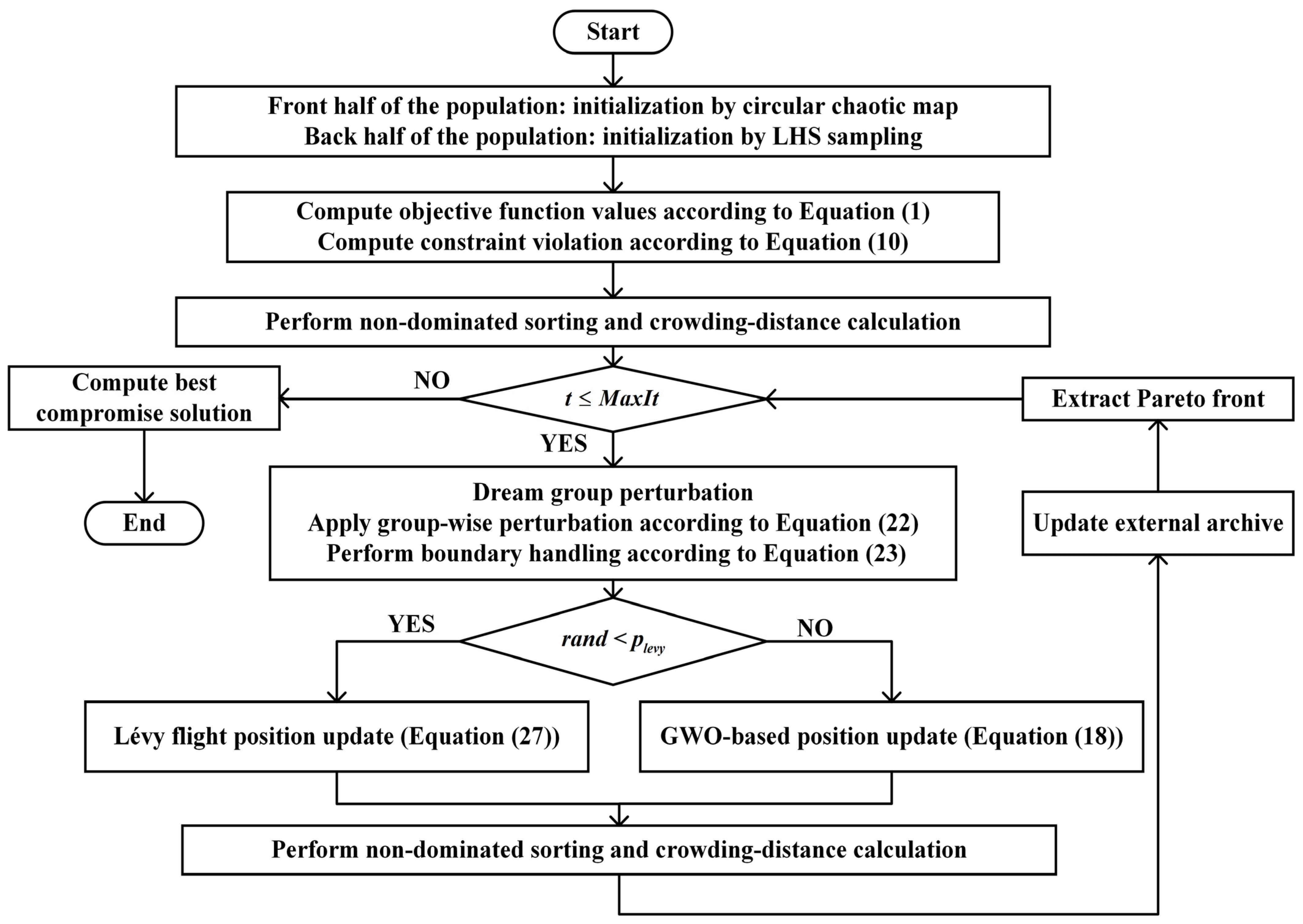
Figure 1 shows the overall procedure of the proposed IMOGWO, from hybrid initialization to Pareto-based selection and compromise solution extraction.

3. Results

3.1. Performance Comparison of IMOGWO on the MW Test Functions

To evaluate IMOGWO on constrained multi-objective optimization problems and lay a foundation for its application to power system dispatch, the algorithm is first tested on the standard MW benchmark suite [18], where the objectives are tightly coupled with the constraints. All two-dimensional problems from the suite—specifically MW1-MW3, MW5-MW7, and MW9-MW13—are used to assess convergence, constraint-handling capability and solution diversity. The results provide insights for parameter settings and inform subsequent studies on more complex power system dispatch scenarios.

3.1.1. Experimental Parameters

To evaluate the performance of the proposed algorithm, seven multi-objective optimization algorithms were selected as comparative benchmarks: MOGWO, AGEMOEA-II [19], PPS [20], ARMOEA [21], MOPSO [4], NSGA-III [22], and NSGA-II [2]. For a fair comparison on the MW benchmark suite, all algorithms were independently run 30 times with a population size of 100 and a maximum of 1000 iterations. The reported IGD and HV values were averaged over the 30 runs. For archive-based algorithms, the external archive size was limited to 100. Algorithm-specific parameters followed the settings recommended in the original references, while all shared parameters were kept identical. The same population size, maximum number of iterations, number of independent runs, and archive size were used for the subsequent dispatch cases.

All numerical experiments were conducted on a personal workstation equipped with an AMD Ryzen 9 7940HX processor (16 cores and 32 logical processors) and 16 GB of RAM, running a 64-bit Microsoft Windows 11 operating system. All algorithms were implemented and executed in MATLAB R2022a (Version 9.12) under the same hardware and software environment.

3.1.2. Evaluation Indicators

To evaluate both the convergence and diversity of the obtained Pareto fronts, two indicators are used: Inverted Generational Distance (IGD) and Hypervolume (HV).

IGD measures the average distance from each point on the true Pareto front $P^{*}$ to its nearest point on the approximated front $P$; smaller IGD values indicate better overall performance. This indicator is defined in Equation (30), where $P^{*}$ denotes the true Pareto front, $P$ is the approximated front generated by the algorithm, and $d(x,y)$ is the Euclidean distance between two solutions.

$$IGD={\displaystyle \frac{1}{\left|P^{*}\right|}}{\displaystyle \sum _{\mathrm{y}\in P^{*},x\in P}\min d(x,y)},$$

(30)

HV quantifies the volume of the objective space dominated by the approximated front $P$ and bounded by a reference point $r$; a larger HV value implies better convergence and a more uniform distribution of solutions. It is defined in Equation (31).

$$HV(P)=VOL\left(\underset{x\in A}{U}\left[f_1(x),r_1^{*}\right]\times \cdots \times \left[f_m(x),r_m^{*}\right]\right),$$

(31)

3.1.3. Comparison of the Results on the MW Test Functions

Table 1. IGD values of eight algorithms on the MW test set.

Test	IMOGWO	MOGWO	AGEMOEA-II	PPS	ARMOEA	MOPSO	NSGA-III	NSGA-II
MW1	0.0048	0.3724	0.0285	0.0070	0.0090	0.1767	0.0151	0.1034
MW2	0.0119	0.1650	0.0285	0.1956	0.0252	0.0246	0.0243	0.0268
MW3	0.0077	0.0461	0.0360	0.0062	0.0085	0.0759	0.2131	0.1185
MW5	0.0054	0.7218	0.3220	0.3795	0.2687	0.2800	0.3363	0.1981
MW6	0.0097	0.6180	0.0287	0.5621	0.0647	0.4085	0.4662	0.3981
MW7	0.0054	0.0179	0.0196	0.0055	0.0676	0.1246	0.1781	0.1816
MW9	0.0120	0.5175	0.0215	0.0831	0.0580	0.1686	0.0651	0.0403
MW10	0.0057	0.5798	0.2500	0.4249	0.1556	0.1460	0.2135	0.1443
MW11	0.0202	0.8348	0.1917	0.0073	0.4524	0.5296	0.5161	0.3523
MW12	0.0061	0.8031	0.0478	0.1007	0.0328	0.1740	0.2865	0.2582
MW13	0.1202	0.1794	0.2422	0.3709	0.4052	0.2675	0.1570	0.2560

reports the mean IGD values of all algorithms on the MW test functions. IMOGWO achieves lower IGD values than the standard MOGWO on all test instances. For example, on MW1, the IGD value is reduced from 0.3724 (MOGWO) to 0.0048 (IMOGWO). Overall, IMOGWO attains the best IGD performance on 9 of the 11 MW test problems, with results comparable to PPS on MW3 and MW11. In contrast, AGEMOEA-II, ARMOEA, and MOPSO consistently yield higher IGD values, indicating that IMOGWO is more effective in solving nonlinearly constrained multi-objective problems and maintains a superior balance between global exploration and local exploitation.

Table 2. HV values of eight algorithms on the MW test set.

Test	IMOGWO	MOGWO	AGEMOEA-II	PPS	ARMOEA	MOPSO	NSGA-III	NSGA-II
MW1	0.5525	0.2125	0.4853	0.4814	0.4817	0.4727	0.4748	0.5286
MW2	0.6835	0.4602	0.5413	0.3499	0.5462	0.5470	0.5473	0.5435
MW3	0.6533	0.4524	0.5261	0.5432	0.5427	0.4640	0.4707	0.5644
MW5	0.3892	0.1064	0.2142	0.2023	0.2230	0.2252	0.2081	0.2449
MW6	0.3846	0.1050	0.2926	0.1035	0.2875	0.1401	0.2163	0.1277
MW7	0.4977	0.4725	0.4063	0.4118	0.3887	0.4666	0.4284	0.4549
MW9	0.2878	0.1511	0.3829	0.3344	0.3601	0.2980	0.3530	0.3689
MW10	0.6647	0.1706	0.3003	0.2146	0.3489	0.3532	0.3206	0.3542
MW11	0.6880	0.3694	0.3982	0.4475	0.3410	0.3139	0.3178	0.3598
MW12	0.5527	0.1302	0.5729	0.5160	0.5826	0.4945	0.0187	0.3447
MW13	0.4568	0.3885	0.3931	0.2979	0.3774	0.3914	0.4219	0.3938

reports the mean HV values of all algorithms on the MW test set. IMOGWO attains the highest HV on 9 of the 11 problems, showing its ability to generate Pareto fronts with good convergence and diversity. It improves the HV over standard MOGWO on every instance—for example, from 0.2125 to 0.5525 on MW1—and outperforms NSGA-II and NSGA-III on 10 of the 11 cases. Although PPS, AGEMOEA-II, ARMOEA, and MOPSO achieve slightly better results on a few individual problems, IMOGWO still provides the best overall HV performance and consistently yields high-quality Pareto-front approximations.

Figure 2, Figure 3, Figure 4 and Figure 5 compare the Pareto fronts of IMOGWO with those of four other algorithms on MW3, MW6, MW7, and MW12. In each plot, red points denote approximate Pareto fronts and the blue curve represents the reference front. On MW3 and MW7, solutions obtained by IMOGWO closely approximate the reference front and provide uniform, dense coverage, whereas other algorithms show gaps or deviations. For the more challenging MW6 and MW12, competing methods often yield sparse or truncated fronts, while IMOGWO still offers a well-converged and diverse approximation. These visual results are consistent with the IGD and HV metrics, confirming the superior convergence and diversity of IMOGWO.

3.2. Application of IMOGWO in EED

To validate the effectiveness and robustness of IMOGWO for power system dispatch, three representative EED test cases [23] with different system scales and characteristics are considered. Cases 1 and 2 model transmission losses explicitly, whereas Case 3 adopts a lossless assumption. Case 1 uses a standard quadratic cost model, while Cases 2 and 3 include valve-point effects to better reflect the non-smooth fuel-cost characteristics of practical generating units.

3.2.1. Case 1

Case 1 uses the standard IEEE 30-bus system, which includes six generating units, a load demand of PD = 2.834 p.u., a base power of 100 MVA, and 21 load buses. In this case, transmission line losses are considered, and the emission function differs slightly from the general form given in Equation (5) and is represented by the following nonlinear model:

$$f_2={\displaystyle \sum _{i=1}^n[0.01({\alpha }_i++{\beta }_i{P}_i+{\gamma }_i{P}_i^2)+{\eta }_i\exp ({\delta }_i{P}_i)]},$$

(32)

In this paper, the compromise solution for each algorithm is selected by an ideal-point-based normalized distance method. The cost and emission values of all non-dominated solutions are normalized to [0, 1] using the best and worst values of each objective, and the solution with the smallest Euclidean distance to the ideal point is chosen as the compromise dispatch scheme.

To evaluate the economic–environmental trade-off across algorithms, this study uses min-max normalization with a weighted composite score. The normalization is defined as follows:

$$x_{norm}={\displaystyle \frac{x-x_{\min }}{x_{\max }-x_{\min }}},$$

(33)

Here, $x_{\min }$ and $x_{\max }$ are the minimum and maximum values of an index among all algorithms. After normalization, all indices lie in [0, 1] and smaller values indicate better performance. The composite score is then calculated as:

$$Score={\omega }_C\times C_{norm}+{\omega }_E\times E_{norm},$$

(34)

The weights for cost (${\omega }_C=0.6$) and emissions (${\omega }_E=0.4$) are set to reflect an engineering decision preference that prioritizes cost while still considering emission reduction. Under this weighting scheme, a lower overall score indicates a better comprehensive performance of the algorithm.

To evaluate the performance of the proposed IMOGWO, six representative algorithms, including MOGWO, ABC-NSGA-II [24], HBB-BC [25], MOPSO, NSGA-III, and NSGA-II, are selected for comparison in the 6-unit system.

Table 3. Comparison of optimal compromise solutions for the 6-unit system (C: $/h; E: ton/h).

Case 1	Optimal Compromise Solution for the 6-Unit System
	IMOGWO	MOGWO	ABC-NSGA-II	HBB-BC	MOPSO	NSGA-III	NSGA-II
1	0.2685	0.2520	0.3039	0.2998	0.2011	0.2565	0.2852
2	0.3892	0.4137	0.3958	0.4213	0.4546	0.3920	0.3777
3	0.5458	0.5463	0.5839	0.5480	0.5743	0.6083	0.5341
4	0.6795	0.6797	0.5924	0.5909	0.7479	0.6686	0.6760
5	0.5407	0.5205	0.5474	0.5393	0.4111	0.5525	0.5726
6	0.4366	0.4483	0.4379	0.4632	0.4872	0.3910	0.4147
C (×102)	6.1685	6.1717	6.2260	6.2378	6.1972	6.1873	6.1713
Cnorm	0.0000	0.0462	0.8298	1.0000	0.4141	0.2713	0.0404
E	0.2000	0.2001	0.1975	0.1971	0.2038	0.2006	0.2000
Enorm	0.4328	0.4478	0.0597	0.0000	1.0000	0.5224	0.4328
Score	0.1731	0.2068	0.5217	0.6000	0.6485	0.3717	0.1974

compares the optimal compromise solutions obtained by these algorithms. The results indicate that IMOGWO achieves the minimum generation cost of 6.1685 × 10², demonstrating its superior economic dispatch performance. For the emission objective, IMOGWO yields a value of 0.2000, which remains competitive although it is not the lowest among all the compared algorithms. Furthermore, IMOGWO attains the lowest normalized weighted score of 0.1731, indicating a better trade-off between fuel cost and pollutant emissions. Therefore, IMOGWO demonstrates superior overall optimization performance among the compared algorithms.

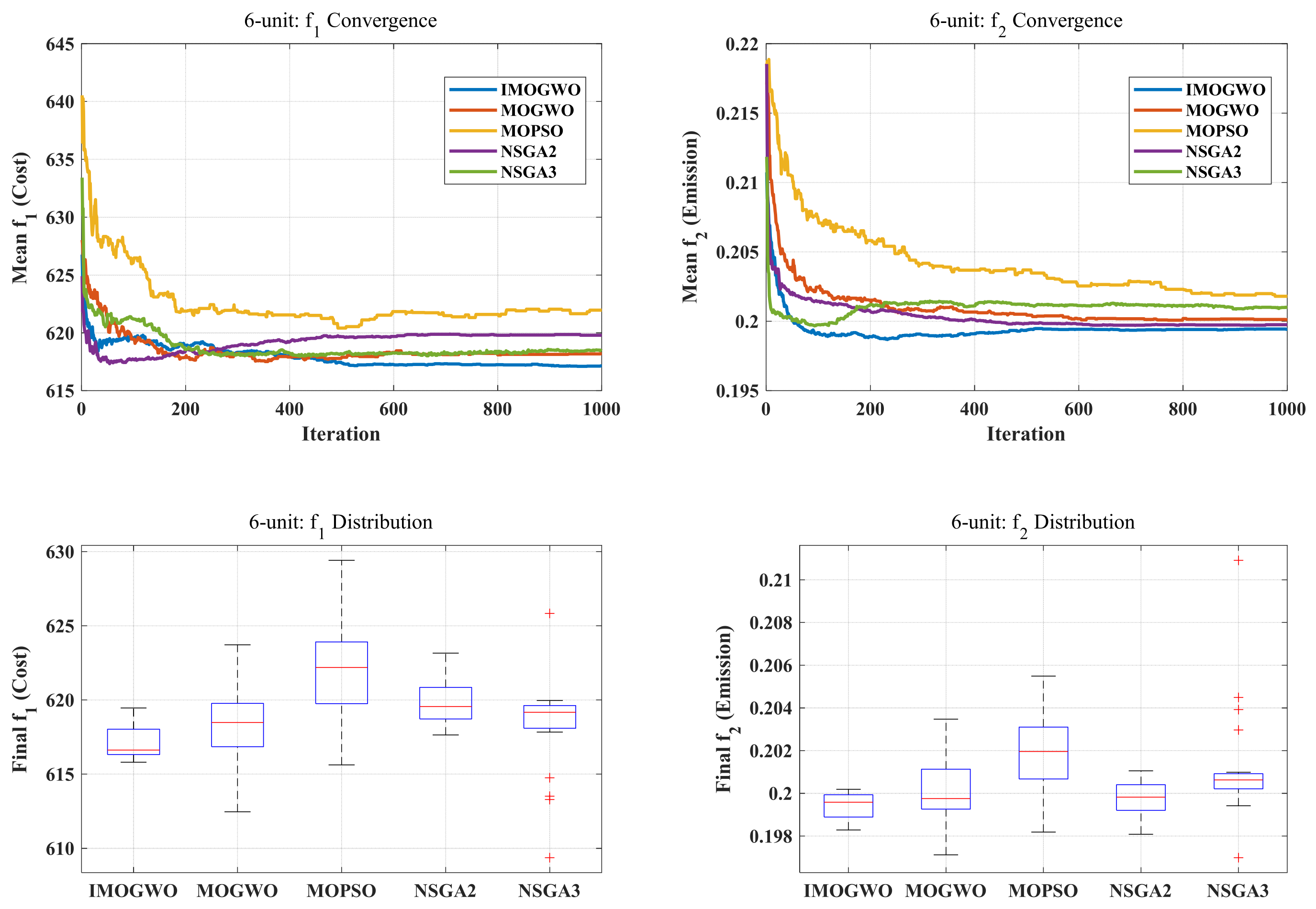
Figure 6 compares the convergence curves and box plots of $f_1$ and $f_2$ for different algorithms in the 6-unit system. The convergence curves show that IMOGWO achieves a faster convergence rate and lower final objective values than the competing algorithms. In addition, the box plots of IMOGWO are more compact and contain fewer outliers, indicating that the proposed method achieves better solution quality and exhibits higher stability and robustness in solving the multi-objective dispatch problem.

Table 4. Wilcoxon rank-sum test results of IMOGWO versus competing algorithms for the 6-unit system.

Comparison 6-Unit	$\mathit{p}$-Value for ${\mathit{f}}_1$	Significance	$\mathit{p}$-Value for ${\mathit{f}}_2$	Significance
IMOGWO vs. MOGWO	1.383 × 10−2	Significant	1.413 × 10−1	Not significant
IMOGWO vs. MOPSO	8.485 × 10−9	Significant	7.599 × 10−7	Significant
IMOGWO vs. NSGA-II	6.518 × 10−9	Significant	7.483 × 10−2	Not significant
IMOGWO vs. NSGA-III	7.659 × 10−5	Significant	7.088 × 10−8	Significant

presents the Wilcoxon rank-sum test results between IMOGWO and the compared algorithms for the 6-unit system. The results show that IMOGWO exhibits statistically significant differences from all the compared algorithms in terms of the $f_1$ objective, whereas statistically significant differences are observed only for some algorithms in terms of the $f_2$ objective. This indicates that, in the small-scale system, the main advantage of IMOGWO lies in its consistent improvement in overall solution performance, particularly in economic optimization, while it also remains competitive with respect to emission optimization.

3.2.2. Case 2

Case 2 considers a 10-unit system with a total load demand of PD = 2000 MW and includes transmission losses, thereby enabling evaluation of the convergence capability and solution quality of the algorithm in a medium-scale setting.

To evaluate the performance of the proposed IMOGWO, six representative algorithms, including MOGWO, GSA [26], MOAOA [27], NSGA-II, NSGA-III, and MOPSO, are selected for comparison in the 10-unit system.

Table 5. Comparison of optimal compromise solutions for the 10-unit system (C: $/h; E: ton/h).

Case 2	Optimal Compromise Solution for the 10-Unit System
	IMOGWO	MOGWO	GSA	MOAOA	NSGA-II	NSGA-III	MOPSO
1	54.9948	54.7562	54.9992	54.9487	51.9515	40.0464	52.7527
2	79.6331	78.2980	79.9586	74.5821	67.2584	63.1774	80.0000
3	86.4567	88.2152	79.4341	79.4294	73.6879	89.7647	74.2543
4	79.4831	85.5268	85.0000	80.6875	91.3554	88.0272	86.1759
5	123.1705	150.0107	142.1063	136.855	134.0522	130.8286	128.2558
6	155.4196	173.6119	166.5670	172.639	174.9504	195.3755	155.6784
7	298.6497	284.0109	292.8749	283.823	289.4350	270.1358	288.836
8	317.1639	317.5142	313.2387	316.341	314.0556	317.1809	305.9999
9	443.2132	422.7529	441.1775	448.592	455.6978	433.3534	442.7738
10	446.2151	428.1385	428.6306	436.429	431.8054	456.0734	470.0000
C (×105)	1.1279	1.1384	1.1349	1.1348	1.1354	1.1403	1.1287
Cnorm	0.0000	0.8468	0.5645	0.5565	0.6048	1.0000	0.0645
E (×103)	4.1887	4.0745	4.1114	4.1248	4.1509	4.1724	4.2066
Enorm	0.8645	0.0000	0.2793	0.3808	0.5783	0.7411	1.0000
Score	0.3458	0.5081	0.4504	0.4862	0.5942	0.8964	0.4387

compares the optimal compromise solutions obtained by these algorithms. The results indicate that IMOGWO achieves the minimum generation cost of 1.1279 × 10⁵, demonstrating its superior economic optimization performance. For the emission objective, IMOGWO yields a value of 4.1887 × 10³, which remains competitive although it is not the lowest among all the compared algorithms. Furthermore, IMOGWO attains the lowest comprehensive score of 0.3458, indicating a better trade-off between generation cost and pollutant emissions. Therefore, IMOGWO demonstrates superior overall optimization performance in the 10-unit system.

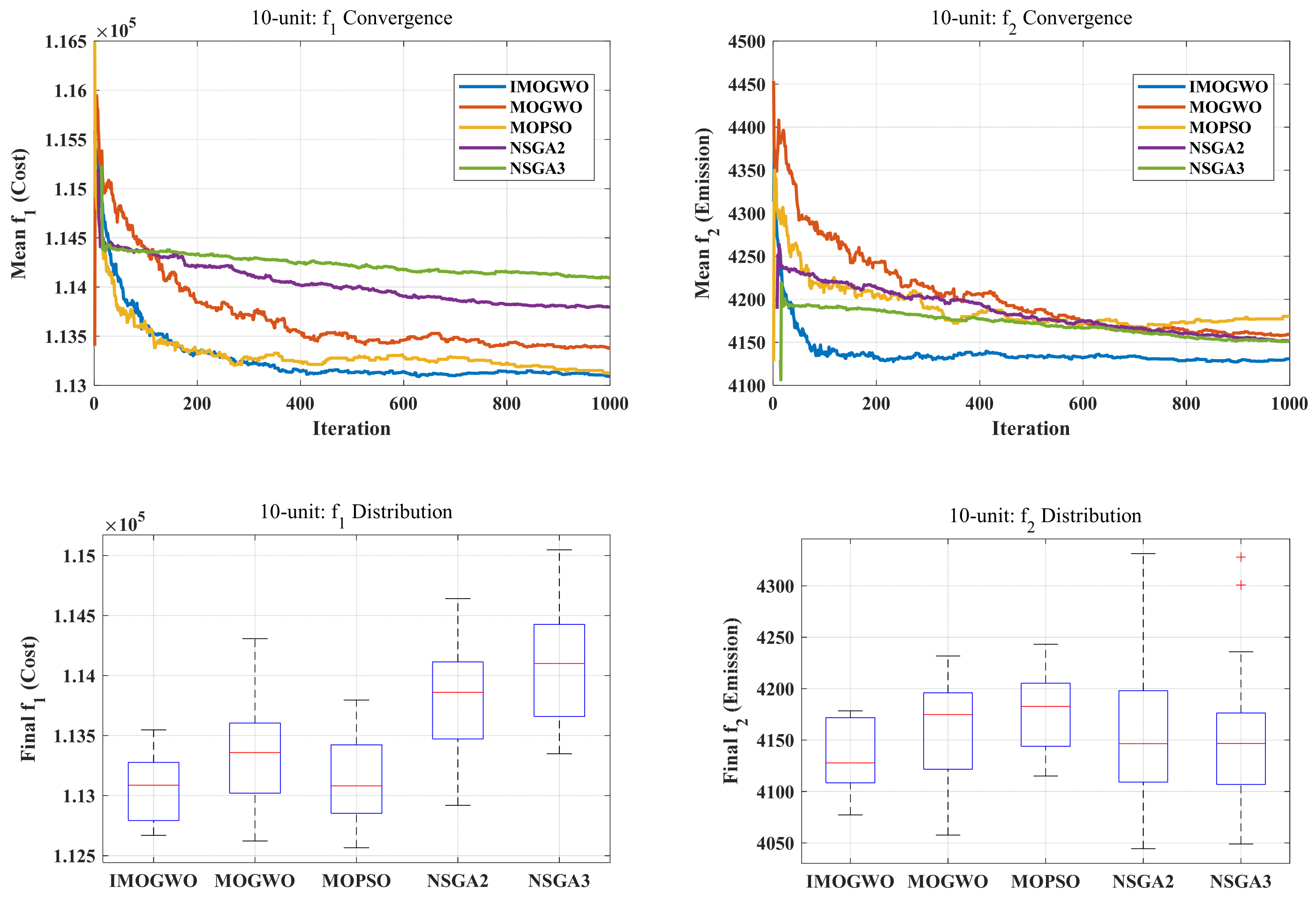
Figure 7 compares the convergence curves and box plots of $f_1$ and $f_2$ for different algorithms in the 10-unit system. As shown by the convergence curves, IMOGWO achieves a rapid decrease in both objective functions during the early stages of the iterative process and maintains a relatively stable convergence trend in the later stages. In terms of the final convergence results, IMOGWO exhibits a more pronounced advantage for the $f_1$ objective and also obtains a competitive final solution for the $f_2$ objective. The box plots further show that the results of IMOGWO are more concentrated for both objectives, indicating that the algorithm has good stability and robustness over multiple independent runs. Overall, IMOGWO demonstrates superior final solution quality and satisfactory operational stability in the 10-unit system, highlighting its comprehensive advantage in solving this problem.

Table 6. Wilcoxon rank-sum test results of IMOGWO versus competing algorithms for the 10-unit system.

Comparison 10-Unit	$\mathit{p}$-Value for ${\mathit{f}}_1$	Significance	$\mathit{p}$-Value for ${\mathit{f}}_2$	Significance
IMOGWO vs. MOGWO	1.695 × 10−2	Significant	1.123 × 10−2	Significant
IMOGWO vs. MOPSO	7.172 × 10−1	Not significant	1.529 × 10−5	Significant
IMOGWO vs. NSGA-II	7.695 × 10−8	Significant	1.858 × 10−1	Not significant
IMOGWO vs. NSGA-III	2.154 × 10−10	Significant	3.042 × 10−1	Not significant

presents the Wilcoxon rank-sum test results between IMOGWO and the competing algorithms for the 10-unit system. The results show that the patterns of statistical significance are not completely consistent across the two objective functions, indicating that different algorithms possess different characteristics in optimizing generation cost and pollutant emissions. Despite this, IMOGWO exhibits statistically competitive performance in both objectives, demonstrating its ability to effectively balance multiple objectives in the medium-scale system while maintaining favorable overall optimization performance.

3.2.3. Case 3

Case 3 considers a 40-unit system, the largest test case, with a total load demand of PD = 10500 MW. This large-scale system is used to further assess the applicability and scalability of IMOGWO in practical power dispatch.

To evaluate the performance of the proposed IMOGWO, six representative algorithms, including MOGWO, MABC [28], BSA [29], MOPSO, NSGA-II, and NSGA-III, are selected for comparison in the 40-unit system.

Table 7. Comparison of optimal compromise solutions for the 40-unit system (C: $/h; E: ton/h).

Case 3	Optimal Compromise Solution for the 40-Unit System
	IMOGWO	MOGWO	MABC	BSA	MOPSO	NSGA-II	NSGA-III
1	110.8373	107.5553	110.7998	111.0281	114.0000	85.8014	83.1745
2	113.9926	109.5551	110.7998	110.9843	89.7101	109.2769	76.337
3	119.8577	112.1955	97.3999	97.5185	120.0000	85.8234	99.3765
4	179.5259	182.9292	174.5504	179.6235	190.0000	169.5193	144.219
5	96.9708	96.2216	87.7999	87.9014	96.6921	81.3308	83.4638
6	139.9829	139.8365	105.3999	139.9362	140.0000	108.1611	129.364
7	300.0000	277.1200	259.5996	299.9973	300.0000	267.3685	268.2199
8	287.3202	295.2827	284.5996	284.8178	282.2527	287.8816	264.2021
9	284.5066	296.6429	284.5996	284.6970	275.0589	276.122	260.592
10	130.0257	204.4095	130.0000	130.0010	204.7925	203.5305	204.1119
11	318.3170	314.9100	318.1921	243.5997	193.9787	307.9518	297.9139
12	318.0315	151.4337	243.5996	243.5861	211.1827	258.2566	315.8201
13	394.4128	396.0851	394.2793	394.3576	318.2122	454.7243	426.1775
14	394.8321	305.0625	394.2793	394.0843	352.7366	404.3537	467.9762
15	394.7984	394.2697	394.2793	394.2627	353.6297	394.0511	432.2521
16	394.4282	398.0610	394.2793	394.3353	233.2071	421.3167	401.6257
17	489.2694	488.4731	399.5195	489.2358	486.0005	403.9537	473.0821
18	489.4006	481.4130	399.5195	489.2747	500.0000	403.7097	474.5953
19	511.3776	487.4508	506.1985	511.2517	511.8026	434.8228	449.9421
20	421.9023	493.6426	506.1985	421.4733	496.6577	496.7127	429.7478
21	433.5167	453.3854	514.1472	433.4452	522.6162	488.3112	469.5908
22	433.5184	442.3346	514.1455	433.5131	507.5438	486.708	448.5529
23	440.1273	442.2315	514.5237	433.5401	550.0000	470.201	450.1410
24	440.9680	434.2167	514.5386	521.7719	476.6285	460.5887	484.7590
25	434.6068	437.1445	433.5196	433.6479	495.7415	503.2189	492.0810
26	433.6996	491.5370	433.5195	433.6179	469.1889	466.3976	450.4623
27	10.0498	39.2613	10.0000	10.0987	10.0000	37.2184	45.0010
28	10.0042	12.6996	10.0000	10.0804	29.9638	36.5524	42.7632
29	10.2264	30.6530	10.0000	10.0058	10.0000	35.8387	40.6864
30	93.7822	89.3795	97.0000	88.0450	86.0271	84.5052	76.1837
31	189.5886	187.3940	159.7330	189.9998	190.0000	126.0283	157.3416
32	162.8088	176.7853	159.7330	189.9849	190.0000	160.0500	167.9751
33	171.5521	160.4591	159.7330	189.9779	180.0169	173.7493	155.7552
34	198.3190	197.6835	200.0000	199.9724	190.1199	181.7347	169.4936
35	199.8172	195.9182	200.0000	199.9822	200.0000	200.0000	172.9190
36	199.6932	200.0000	200.0000	199.9999	200.0000	199.6179	138.0640
37	107.7459	98.6682	89.1141	89.2085	85.3279	108.1921	91.1040
38	109.5345	97.7090	89.1141	109.9997	42.3246	62.9241	81.7924
39	108.6564	90.7743	89.1141	109.9719	110.0000	82.2445	91.7857
40	422.0178	488.4867	506.1879	511.1699	490.4285	481.8606	490.7761
C (×105)	1.2546	1.2718	1.2420	1.2418	1.2670	1.3049	1.3181
Cnorm	0.1678	0.3932	0.0026	0.0000	0.3303	0.8270	1.0000
E (×105)	2.0341	2.2534	2.3526	2.3354	3.1613	2.2519	2.2758
Enorm	0.0000	0.1946	0.2826	0.2673	1.0000	0.1932	0.2144
Score	0.1007	0.3137	0.1146	0.1069	0.5982	0.5735	0.6858

compares the optimal compromise solutions obtained by these algorithms. The results indicate that IMOGWO achieves the best performance in terms of the emission objective, with an emission value of 2.0341 × 10⁵, while maintaining a relatively favorable generation cost. Based on the normalized weighted score, IMOGWO attains the lowest comprehensive score of 0.1007, indicating that it achieves a better overall trade-off between generation cost and pollutant emissions. Overall, IMOGWO demonstrates strong overall optimization capability in the 40-unit system.

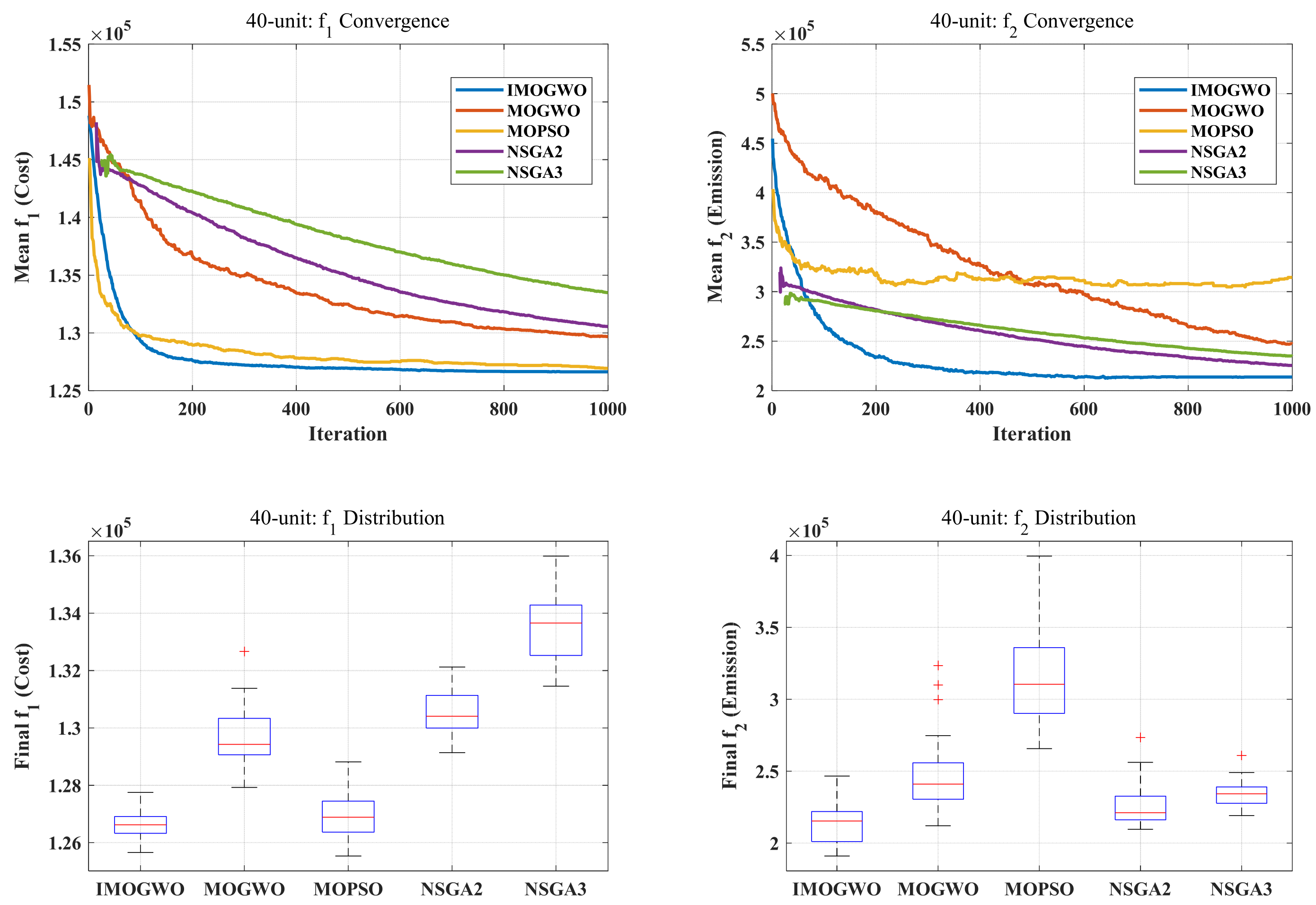
Figure 8 presents the convergence curves and box plots of $f_1$ and $f_2$ for different algorithms in the 40-unit system. The results show that IMOGWO achieves a faster convergence rate for both objective functions and attains superior final convergence performance, particularly for the emission objective $f_2$. In addition, the box plots of IMOGWO exhibit lower median values and more compact distributions, indicating that the algorithm maintains good solution quality, stability, and robustness over multiple independent runs in the large-scale system. Overall, IMOGWO demonstrates superior final solution quality and strong comprehensive optimization capability in the 40-unit system.

Table 8. Wilcoxon rank-sum test results of IMOGWO versus competing algorithms for the 40-unit system.

Comparison 40-Unit	$\mathit{p}$-Value for ${\mathit{f}}_1$	Significance	$\mathit{p}$-Value for ${\mathit{f}}_2$	Significance
IMOGWO vs. MOGWO	3.020 × 10−11	Significant	9.063 × 10−8	Significant
IMOGWO vs. MOPSO	1.023 × 10−1	Significant	9.063 × 10−8	Significant
IMOGWO vs. NSGA-II	1.023 × 10−1	Not significant	3.020 × 10−11	Significant
IMOGWO vs. NSGA-III	3.020 × 10−11	Significant	4.033 × 10−3	Significant

presents the Wilcoxon rank-sum test results between IMOGWO and the compared algorithms for the 40-unit system. The results show that, as the system scale increases, IMOGWO still exhibits statistically significant differences from most of the compared algorithms, with a more pronounced advantage for the $f_2$ objective. This indicates that IMOGWO remains highly effective and statistically competitive in large-scale systems. Its overall performance does not deteriorate significantly as the problem size increases, which further confirms the applicability and effectiveness of the proposed algorithm across systems of different scales.

3.3. Application of IMOGWO in Dynamic Economic Emission Dispatch

Building on the validation of IMOGWO in the static 10-unit system, the proposed algorithm is further applied to the dynamic economic emission dispatch (DEED) [30] problem to evaluate its optimization capability under time-coupled constraints. Compared with static EED, DEED is more consistent with the actual operation of power systems because it requires the simultaneous consideration of fuel cost, pollutant emissions, power balance constraints, transmission losses, and unit ramp-rate constraints over multiple dispatch periods. Consequently, the DEED problem is associated with higher computational complexity. To this end, a dynamic 10-unit system is selected as the test case to assess the convergence performance, solution quality, and operational stability of the proposed algorithm in a medium-scale dynamic scenario. A 24 h scheduling horizon is considered, with a dispatch interval of 1 h. The unit parameters and load demand data for each time period are taken from [30] to ensure the consistency of the test case and the reproducibility of the experimental results. To improve the reliability of the conclusions, all algorithms are independently executed 30 times under the same parameter settings, and their performance is comprehensively evaluated using convergence curves, box plots, and the Wilcoxon rank-sum test.

Compared with static EED, DEED extends single-period generation scheduling into a multi-period coordinated dispatch problem. Let $P_i^t$ denote the power output of unit $i$ during dispatch period $t$. Then, the two objective functions of the dynamic model, namely the total fuel cost and total pollutant emissions over the entire scheduling horizon, can be expressed as follows:

$$F_1={\displaystyle \sum _{t=1}^T{f}_1^t},$$

(35)

$$F_2={\displaystyle \sum _{t=1}^T{f}_2^t},$$

(36)

Here, $f_1^t$ denotes the fuel-cost function with valve-point effects at dispatch period $t$, and $f_2^t$ denotes the pollutant emission function at dispatch period $t$. The specific forms of these two functions are the same as those given in Equations (4) and (5), respectively, except that they are accumulated over the entire scheduling horizon in the dynamic dispatch model.

The power balance constraint and the generation output limits have essentially the same forms as those in the static EED model, but they must be satisfied at every dispatch period in DEED. In addition, to reflect the dynamic operating characteristics of generating units, ramp-rate constraints must also be satisfied between two consecutive time periods. Specifically, the increase or decrease in unit output between adjacent dispatch periods cannot exceed the corresponding ramp-up and ramp-down limits, which can be expressed as follows:

$$P_i^t-P_i^{t-1}\le U{R}_i,i=1,2,\dots ,N;t=2,3,\dots ,T,$$

(37)

$$P_i^{t-1}-P_i^t\le D{R}_i,i=1,2,\dots ,N;t=2,3,\dots ,T,$$

(38)

Here, $U{R}_i$ and $D{R}_i$ denote the ramp-up and ramp-down limits of unit $i$, respectively. These observations indicate that DEED not only requires the coordination of economic and environmental objectives within each dispatch period but also involves the dynamic coupling relationships between adjacent periods. As a result, higher requirements are imposed on the global search capability, constraint-handling ability, and robustness of the optimization algorithm.

To evaluate the performance of the proposed IMOGWO, six representative algorithms, including MOGWO, PSO-CSC [31], MOPSO, MODE [32], NSGA-III, and NSGA-II, are selected for comparison in the dynamic 10-unit system.

Table 9. Comparison of optimal compromise solutions for the dynamic 10-unit system (C: $/24 h; E: lb/24 h).

DEED	Optimal Compromise Solution for the Dynamic 10-Unit System
	IMOGWO	MOGWO	PSO-CSC	MOPSO	MODE	NSGA-III	NSGA-II
C (×106)	2.5215	2.5327	2.5247	2.5558	2.5224	2.5295	2.5246
Cnorm	0.0000	0.3265	0.0933	1.0000	0.0262	0.2332	0.0904
E (×105)	2.9900	3.1566	3.0524	3.094	3.0997	3.0149	3.0256
Enorm	0.0000	1.0000	0.3745	0.6242	0.6585	0.1495	0.2137
Score	0.0000	0.5959	0.2058	0.8497	0.2791	0.1997	0.1397

presents the optimal compromise solutions obtained by these algorithms. The results show that IMOGWO achieves the lowest values for both fuel cost and pollutant emissions, with a cost of 2.5215 × 10⁶ and an emission value of 2.9900 × 10⁵, respectively. Since IMOGWO attains the minimum values for both normalized indicators, its comprehensive score reaches 0.0000, indicating that it simultaneously achieves the best economic and environmental performance among all the compared algorithms. Compared with the results obtained for the static system, these findings demonstrate that IMOGWO not only maintains strong optimization capability in the dynamic dispatch environment but also exhibits better adaptability to time-coupled constraints.

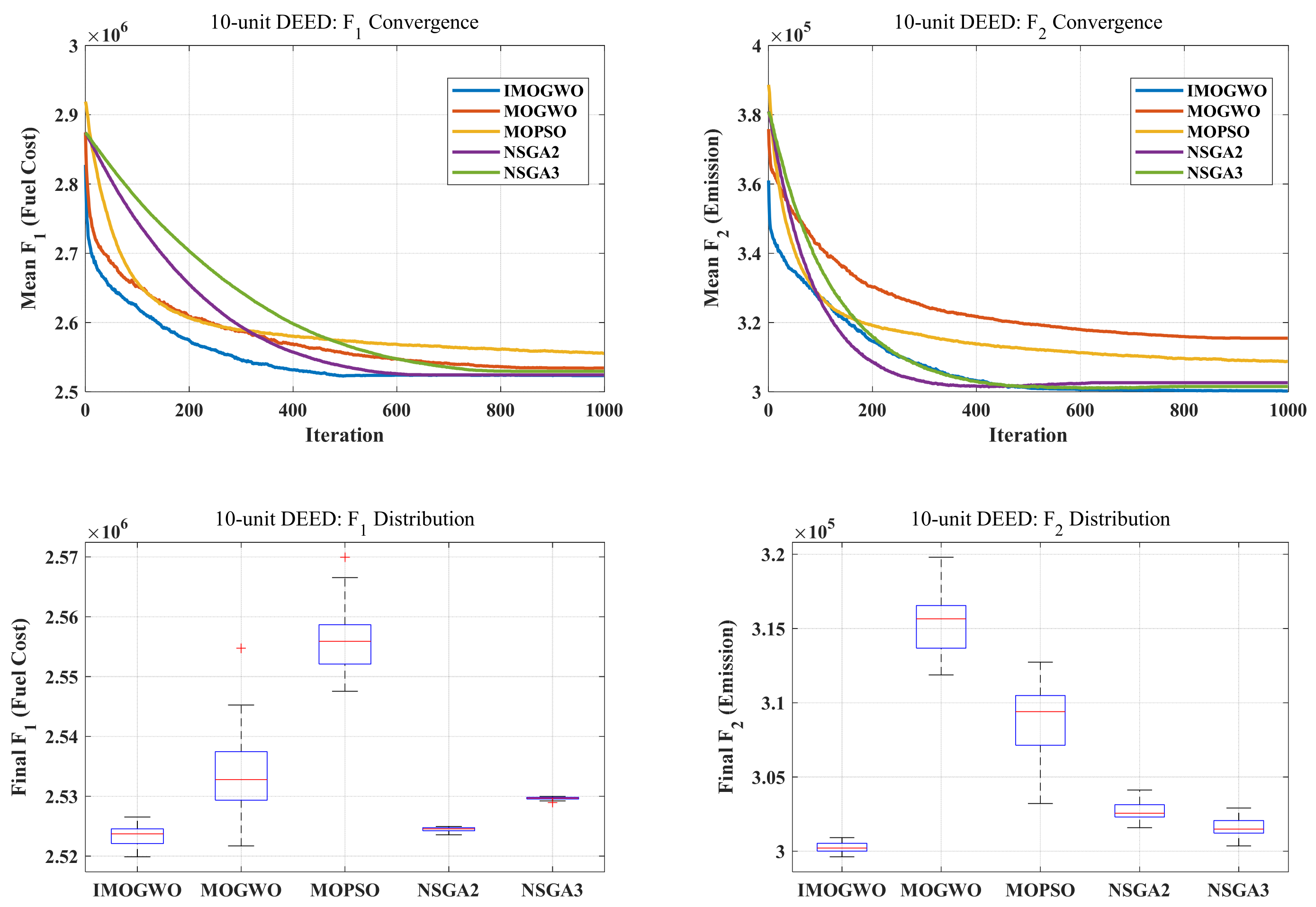
Figure 9 presents the convergence curves and box plots of the objective functions $F_1$ and $F_2$ for the dynamic 10-unit system. The results show that IMOGWO exhibits strong search capability during both the early and middle stages of the iterative process, enabling it to approach high-quality solution regions rapidly while maintaining a relatively stable convergence trend in the later stages. This demonstrates that the proposed algorithm possesses good global search capability and convergence efficiency for the dynamic dispatch problem. In addition, the box plots show that the final solutions obtained by IMOGWO over multiple independent runs are more concentrated, with lower median values. In particular, IMOGWO shows better stability and robustness for the fuel-cost objective. Overall, these results indicate that the proposed algorithm not only achieves high-quality solutions for the DEED problem but also exhibits strong consistency and reliability.

Table 10. Wilcoxon rank-sum test results of IMOGWO versus competing algorithms for the 10-unit dynamic system.

Comparison	$\mathit{p}$-Value for ${\mathit{F}}_1$	Significance	$\mathit{p}$-Value for ${\mathit{F}}_2$	Significance
IMOGWO vs. MOGWO	3.820 × 10−10	Significant	3.020 × 10−11	Significant
IMOGWO vs. MOPSO	3.020 × 10−11	Significant	3.020 × 10−11	Significant
IMOGWO vs. NSGA-II	6.972 × 10−3	Significant	3.020 × 10−11	Significant
IMOGWO vs. NSGA-III	3.020 × 10−11	Significant	8.891 × 10−10	Significant

presents the Wilcoxon rank-sum test results between IMOGWO and the compared algorithms for the dynamic 10-unit system. The results show that, for both $F_1$ and $F_2$, the differences between IMOGWO and all the compared algorithms are statistically significant. These findings indicate that IMOGWO is able to maintain stable optimization performance under dynamic constraints, demonstrating strong adaptability to dynamic environments and a clear overall competitive advantage.

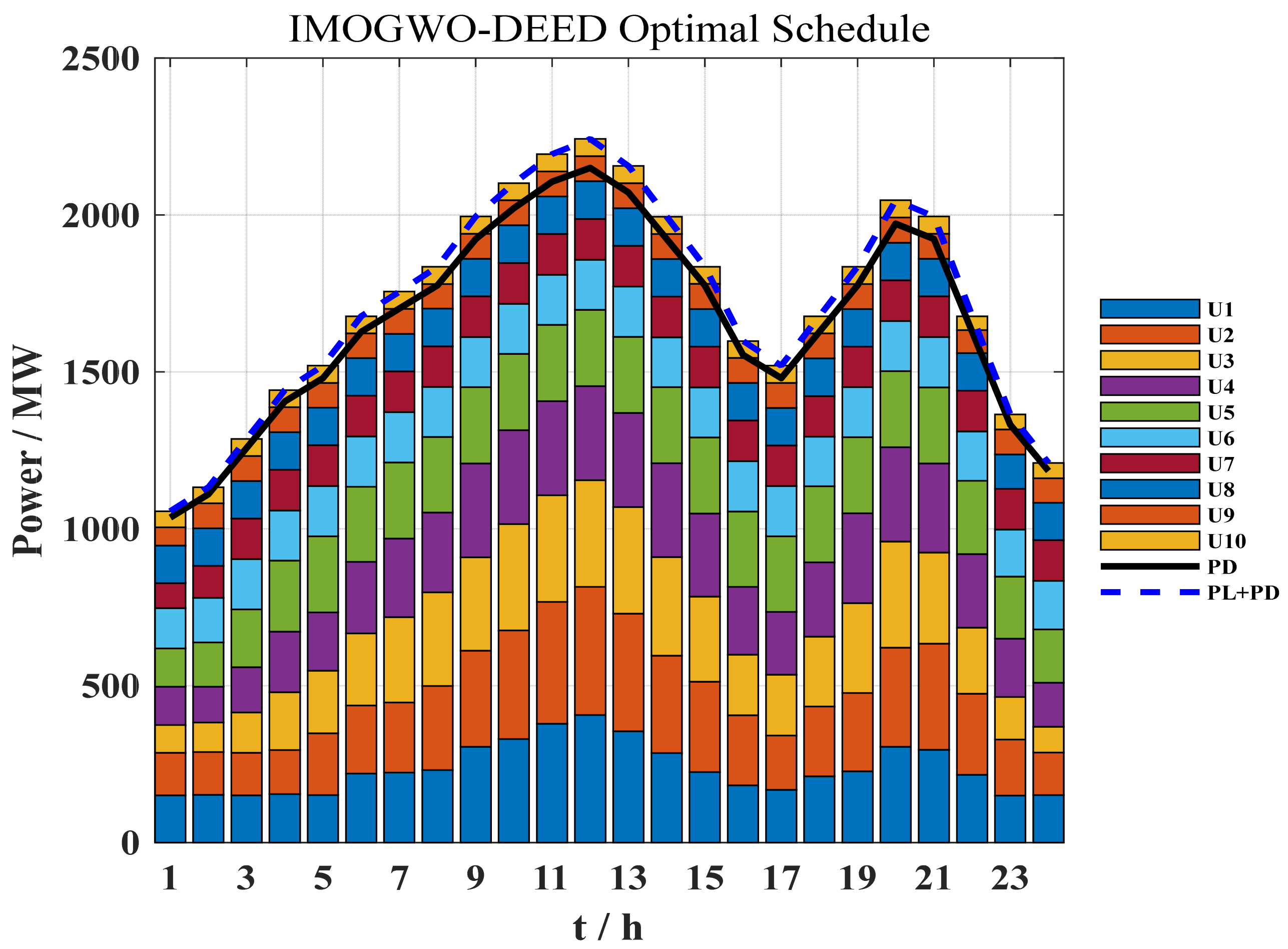
To further illustrate the specific dispatch results obtained by IMOGWO in the dynamic scheduling scenario,

Table 11. Hourly generation schedule of the 10-unit dynamic system (MW).

t	P1	P2	P3	P4	P5	P6	P7	P8	P9	P10	Loss
1	150.9	135.0	88.6	122.5	121.4	129	79.1	119.7	58.2	51.1	19.6
2	152.0	136.3	94.7	113.4	141.5	142.4	101.5	120.0	79.9	50.9	22.5
3	150.6	135.6	128.1	144.7	184.3	160	129.7	119.2	79.7	54.6	28.5
4	154.8	139.8	184.3	193.6	226.1	159.4	130.0	119.6	79.7	54.3	35.6
5	151.3	197.4	199.3	185.7	242.6	160.0	129.9	119.9	78.8	54.9	39.9
6	219.9	216.9	230.1	228.2	239.2	160.0	129.7	119.9	79.2	54.1	49.1
7	222.7	223.4	272.2	250.5	242.8	159.8	130.0	120.0	79.8	54.6	53.8
8	231.0	267.8	298.9	253.9	240.9	159.6	129.6	119.9	78.8	54.8	59.3
9	305.4	306.4	297.3	299.5	242.8	160.0	129.6	119.7	80.0	54.7	71.1
10	329.7	346.1	339.5	299.1	243.0	159.9	129.7	120.0	79.8	54.6	79.6
11	378.8	388.2	340.0	299.9	243.0	160.0	130.0	119.2	79.9	54.8	87.9
12	406.5	408.3	340.0	299.8	243.0	160.0	130.0	120.0	80.0	54.9	92.5
13	354.6	374.9	339.6	300.0	242.8	160.0	130.0	120.0	80.0	54.7	84.4
14	285.4	310.1	314.3	299.0	242.6	159.1	129.8	119.5	80.0	55.0	70.9
15	224.9	287.4	271.2	265.1	242.5	159.7	129.9	119.9	80.0	54.8	59.4
16	182.8	223.1	192.7	216.7	240.1	159.9	130.0	119.4	79.9	54.0	44.5
17	167.7	173.6	193.4	200.7	240.8	159.8	129.3	119.7	79.8	55.0	39.8
18	211.4	222.5	222.3	236.8	242.3	158.3	129.5	119.9	79.9	54.3	49.1
19	226.7	249.7	286.4	286.5	242.9	159.2	129.1	119.8	79.6	55.0	59.0
20	305.2	315.7	338.8	300.0	242.5	159.9	129.8	120.0	80.0	55.0	74.9
21	295.6	338.0	290.7	283.5	242.9	160.0	129.8	120.0	79.8	55.0	71.4
22	215.8	258.3	210.9	234.8	233.2	157.7	129.7	119.7	73.6	44.0	49.5
23	150.1	178.4	135.8	185.5	197.7	150.3	129.6	109.2	80.0	47.7	32.2
24	151.7	135.4	82.0	140.4	169.6	154.7	130.0	118.8	78.6	48.2	25.4

presents the hourly generation outputs of the 10-unit system over the 24 h scheduling horizon, together with the corresponding transmission losses, as determined by the IMOGWO method. Figure 10 shows the corresponding stacked generation profiles and the variation in system load demand. As shown in Figure 10, the generating units achieve a reasonable power allocation under different load levels, and the total power output can effectively satisfy both the system load demand and transmission loss requirements. These results indicate that the dispatch scheme obtained by IMOGWO has good feasibility and practical applicability.

In summary, IMOGWO exhibits superior convergence performance, solution quality, and statistical stability in the dynamic 10-unit system. Subject to the dynamic constraints, the proposed algorithm can effectively balance the two conflicting objectives of fuel cost and pollutant emissions, thereby demonstrating its effectiveness and applicability in solving the dynamic economic emission dispatch problem.

4. Discussion

The superior performance of IMOGWO can be mainly attributed to the coordinated effect of its four improvement strategies. The hybrid initialization scheme improves the diversity of the initial population, the dream-inspired group perturbation mechanism enhances global exploration, the nonlinearly decreasing convergence factor promotes a better balance between exploration and exploitation, and the Lévy flight-based update strategy helps the algorithm escape local optima. These characteristics are particularly beneficial for solving EED and DEED problems, which are highly constrained and strongly non-convex. In addition, the favorable convergence behavior and compact box-plot distributions indicate that the proposed method is not only effective in obtaining high-quality solutions, but also reliable over repeated runs. Nevertheless, the present study is still limited to several benchmark systems and fixed objective-weight settings, and uncertainties associated with renewable generation and load fluctuations are not explicitly considered. Therefore, further research should focus on integrating uncertainty modeling and robust optimization to improve the practical applicability of IMOGWO in more realistic power system environments.

5. Conclusions

This paper proposes an improved multi-objective Grey Wolf Optimizer (IMOGWO) for solving the economic emission dispatch (EED) problem, which is characterized by strong non-convexity, objective conflicts, and multiple operational constraints. The effectiveness of the proposed method is validated on static 6-unit, 10-unit, and 40-unit systems, as well as on a dynamic 10-unit system. The results demonstrate that IMOGWO achieves competitive or superior overall performance in terms of generation cost, pollutant emissions, convergence behavior, Pareto solution quality, and robustness when compared with several existing multi-objective optimization algorithms. These results indicate that IMOGWO is capable of providing high-quality compromise dispatch solutions that effectively balance economic efficiency and environmental objectives. Future work will focus on incorporating uncertainty modeling and robust optimization to further enhance the applicability of IMOGWO in power systems with high penetrations of renewable energy.

References

1. Nourianfar, H.; Abdi, H. Environmental/Economic Dispatch Using a New Hybridizing Algorithm Integrated with an Effective Constraint Handling Technique. Sustainability 2022, 14, 3173. [Google Scholar] [CrossRef] [Scilit]
2. Deb, K.; Pratap, A.; Agarwal, S.; Meyarivan, T. A fast and elitist multiobjective genetic algorithm: NSGA-II. IEEE Trans. Evol. Comput. 2002, 6, 182–197. [Google Scholar] [CrossRef] [Scilit]
3. Basu, M. Economic environmental dispatch using multi-objective differential evolution. Appl. Soft Comput. 2011, 11, 2845–2853. [Google Scholar] [CrossRef] [Scilit]
4. Abido, M.A. Multiobjective particle swarm optimization for environmental/economic dispatch problem. Electr. Power Syst. Res. 2009, 79, 1105–1113. [Google Scholar] [CrossRef] [Scilit]
5. Kadali, K.S.; Veeraswamy, M.; Ponnusamy, M.; Jawalkar, V.R. Linear interpolated multi-objective economic emission scheduling using grey wolf optimizer: A strategic balance and solution with diverse load pattern. COMPEL-Int. J. Comput. Math. Electr. Electron. Eng. 2022, 41, 427–454. [Google Scholar] [CrossRef] [Scilit]
6. Almalaq, A.; Guesmi, T.; Albadran, S. A Hybrid Chaotic-Based Multiobjective Differential Evolution Technique for Economic Emission Dispatch Problem. Energies 2023, 16, 4554. [Google Scholar] [CrossRef] [Scilit]
7. Xia, A.M.; Wu, X.D.; Bai, Y.J. A new multi-objective hybrid optimization algorithm for wind-thermal dynamic economic emission power dispatch. Int. Trans. Electr. Energy Syst. 2021, 31, e12966. [Google Scholar] [CrossRef] [Scilit]
8. Dong, R.Y.; Ma, L.; Chen, H.L.; Heidari, A.A.; Liang, G.X. Hybrid kernel search and particle swarm optimization with Cauchy perturbation for economic emission load dispatch with valve point effect. Front. Energy Res. 2023, 10, 1061408. [Google Scholar] [CrossRef] [Scilit]
9. Li, L.-L.; Shen, Q.; Tseng, M.-L.; Luo, S. Power system hybrid dynamic economic emission dispatch with wind energy based on improved sailfish algorithm. J. Clean. Prod. 2021, 316, 128318. [Google Scholar] [CrossRef] [Scilit]
10. Zhu, Z.J.; Wang, J.; Baloch, M.H. Dynamic economic emission dispatch using modified NSGA-II. Int. Trans. Electr. Energy Syst. 2016, 26, 2684–2698. [Google Scholar] [CrossRef] [Scilit]
11. Yu, J.; Kim, C.-H.; Wadood, A.; Khurshiad, T.; Rhee, S.-B. A Novel Multi-Population Based Chaotic JAYA Algorithm with Application in Solving Economic Load Dispatch Problems. Energies 2018, 11, 1946. [Google Scholar] [CrossRef] [Scilit]
12. Mousavi, S.H.; Abdolahi, A.; Khavar, S.C.; Kalantari, N.T. Optimal trade-off between cost and emission for energy hubs management in smart residential buildings. In Proceedings of the 2023 27th International Electrical Power Distribution Networks Conference (EPDC), Mashhad, Iran, 2–4 May 2023. [Google Scholar] [CrossRef] [Scilit]
13. Shahri, H.Y.; Hosseini, S.A.; Pourhossein, J. Multi-objective evolutionary method for multi-area dynamic emission/economic dispatch considering energy storage and renewable energy units. Heliyon 2024, 10, e37476. [Google Scholar] [CrossRef] [Scilit]
14. Lang, Y.; Gao, Y. Dream Optimization Algorithm (DOA): A novel metaheuristic optimization algorithm inspired by human dreams and its applications to real-world engineering problems. Comput. Methods Appl. Mech. Eng. 2025, 436, 117718. [Google Scholar] [CrossRef] [Scilit]
15. Bai, Y.J.; Wu, X.D.; Xia, A.M. An enhanced multi-objective differential evolution algorithm for dynamic environmental economic dispatch of power system with wind power. Energy Sci. Eng. 2021, 9, 316–329. [Google Scholar] [CrossRef] [Scilit]
16. Mirjalili, S.; Mirjalili, S.M.; Lewis, A. Grey Wolf Optimizer. Adv. Eng. Softw. 2014, 69, 46–61. [Google Scholar] [CrossRef] [Scilit]
17. Chegini, S.N.; Bagheri, A.; Najafi, F. PSOSCALF: A new hybrid PSO based on Sine Cosine Algorithm and Levy flight for solving optimization problems. Appl. Soft Comput. 2018, 73, 697–726. [Google Scholar] [CrossRef] [Scilit]
18. Ma, Z.; Wang, Y. Evolutionary Constrained Multiobjective Optimization: Test Suite Construction and Performance Comparisons. IEEE Trans. Evol. Comput. 2019, 23, 972–986. [Google Scholar] [CrossRef] [Scilit]
19. Panichella, A. An improved Pareto front modeling algorithm for large-scale many-objective optimization. In Proceedings of the Genetic and Evolutionary Computation Conference, Boston, MA, USA, 9–13 July 2022; pp. 565–573. [Google Scholar] [CrossRef] [Scilit]
20. Fan, Z.; Li, W.; Cai, X.; Li, H.; Wei, C.; Zhang, Q.; Deb, K.; Goodman, E. Push and pull search for solving constrained multi-objective optimization problems. Swarm Evol. Comput. 2019, 44, 665–679. [Google Scholar] [CrossRef] [Scilit]
21. Tian, Y.; Cheng, R.; Zhang, X.; Cheng, F.; Jin, Y. An Indicator-Based Multiobjective Evolutionary Algorithm With Reference Point Adaptation for Better Versatility. IEEE Trans. Evol. Comput. 2018, 22, 609–622. [Google Scholar] [CrossRef] [Scilit]
22. Deb, K.; Jain, H. An Evolutionary Many-Objective Optimization Algorithm Using Reference-Point-Based Nondominated Sorting Approach, Part I: Solving Problems with Box Constraints. IEEE Trans. Evol. Comput. 2014, 18, 577–601. [Google Scholar] [CrossRef] [Scilit]
23. Zou, D.X.; Li, S.; Li, Z.Y.; Kong, X.Y. A new global particle swarm optimization for the economic emission dispatch with or without transmission losses. Energy Convers. Manag. 2017, 139, 45–70. [Google Scholar] [CrossRef] [Scilit]
24. Sutar, M.; Jadhav, H.T. A modified artificial bee colony algorithm based on a non-dominated sorting genetic approach for combined economic-emission load dispatch problem. Appl. Soft Comput. 2023, 144, 110433. [Google Scholar] [CrossRef] [Scilit]
25. Labbi, Y.; Ben Attous, D. Environmental/economic power dispatch using a Hybrid Big Bang–Big Crunch optimization algorithm. Int. J. Syst. Assur. Eng. Manag. 2014, 5, 602–610. [Google Scholar] [CrossRef] [Scilit]
26. Güvenç, U.; Sönmez, Y.; Duman, S.; Yörükeren, N. Combined economic and emission dispatch solution using gravitational search algorithm. Sci. Iran. 2012, 19, 1754–1762. [Google Scholar] [CrossRef] [Scilit]
27. Hao, W.-K.; Wang, J.-S.; Li, X.-D.; Liu, Y.; Zhu, J.-H.; Zhang, M.; Wang, M. Multi-objective arithmetic optimization algorithm with random searching strategies to solve combined economic emission dispatch problem. Comput. Ind. Eng. 2024, 195, 110434. [Google Scholar] [CrossRef] [Scilit]
28. Secui, D.C. A new modified artificial bee colony algorithm for the economic dispatch problem. Energy Convers. Manag. 2015, 89, 43–62. [Google Scholar] [CrossRef] [Scilit]
29. Bhattacharjee, K.; Bhattacharya, A.; Halder Nee Dey, S. Backtracking search optimization based economic environmental power dispatch problems. Int. J. Electr. Power Energy Syst. 2015, 73, 830–842. [Google Scholar] [CrossRef] [Scilit]
30. Qian, S.Q.; Wu, H.H.; Xu, G.F. An improved particle swarm optimization with clone selection principle for dynamic economic emission dispatch. Soft Comput. 2020, 24, 15249–15271. [Google Scholar] [CrossRef] [Scilit]
31. Huang, H.; Lv, L.; Ye, S.; Hao, Z. Particle swarm optimization with convergence speed controller for large-scale numerical optimization. Soft Comput. 2019, 23, 4421–4437. [Google Scholar] [CrossRef] [Scilit]
32. Basu, M. Multi-objective Differential Evolution for Dynamic Economic Emission Dispatch. Int. J. Emerg. Electr. Power Syst. 2014, 15, 141–150. [Google Scholar] [CrossRef]
Figure 1. Flowchart of the IMOGWO algorithm.
Electricity 07 00090 g001
Figure 2. Pareto-front comparison of IMOGWO with other algorithms on MW3.
Electricity 07 00090 g002
Figure 3. Pareto-front comparison of IMOGWO with other algorithms on MW6.
Electricity 07 00090 g003
Figure 4. Pareto-front comparison of IMOGWO with other algorithms on MW7.
Electricity 07 00090 g004
Figure 5. Pareto-front comparison of IMOGWO with other algorithms on MW12.
Electricity 07 00090 g005
Figure 6. Convergence curves and box plots of f 1 and f 2 for the 6-unit system.
Electricity 07 00090 g006
Figure 7. Convergence curves and box plots of f 1 and f 2 for the 10-unit system.
Electricity 07 00090 g007
Figure 8. Convergence curves and box plots of f 1 and f 2 for the 40-unit system.
Electricity 07 00090 g008
Figure 9. Convergence curves and box plots of F 1 and F 2 for the 10-unit dynamic system.
Electricity 07 00090 g009
Figure 10. Unit outputs and load demand curve of the 10-unit dynamic system.
Electricity 07 00090 g010