Discrete-Time Integral Sliding Mode Control with Optimal Reaching Gain: Application to a Photovoltaic Battery Charging System

Abstract

Discrete-time sliding mode controllers that utilize saturation-based reaching laws require a gain that ensures contraction within the boundary layer in the presence of multiplicative gain uncertainty. The conventional fixed-gain approach does not maintain this property at moderate uncertainty levels. This work introduces a family of admissible reaching gains and identifies a unique optimal gain that guarantees a specified worst-case contraction. The proposed method offers a closed-form solution to the worst-case contraction problem over the gain-uncertainty interval and determines the optimal contraction factor for the saturation-based reaching law for any finite uncertainty ratio. The optimal gain is integrated into a discrete-time integral sliding-mode framework, thereby eliminating the reaching phase. Furthermore, a past-step disturbance estimator with a confidence factor is introduced to prevent error amplification, which reduces the quasi-sliding band from first to second order in the sampling period when the realized gain approximates its nominal value. The effectiveness of the proposed approach is validated through its application to a photovoltaic battery-charging system with a DC–DC boost converter, achieving robust inductor-current regulation across three battery banks under varying irradiance conditions in a switching-level model with parasitic elements.

1. Introduction

Sliding mode control (SMC) is a well-established robust control methodology for uncertain nonlinear systems [1,2,3]. In continuous time, SMC achieves exact compensation of matched bounded perturbations in finite time. However, digital implementation via sample-and-hold limits the existence of an ideal sliding mode [4]. As a result, the trajectory is confined to a neighborhood of the sliding surface known as the quasi-sliding mode band [5].

Several discrete-time SMC formulations have been proposed to address the intrinsic limitations of sampling. Sarpturk et al. [6] investigated stability conditions for discrete-time systems with matched uncertainties. Furuta [7] developed a discrete-time sliding mode controller for linear systems with parametric uncertainties. Misawa [8] developed a saturation-based controller that handles both unmatched uncertainties and uncertain control gain. This controller established boundary-layer attractivity through a discrete Lyapunov argument. Bartoszewicz [9] proposed reaching laws tailored to discrete-time implementations, and Bandyopadhyay and Janardhanan [10] extended the framework to multirate output feedback. More recently, implicit discretization methods have been shown to eliminate numerical chattering entirely [11,12,13]. Reaching law approaches have also been extensively studied; Gao et al. [5] introduced the quasi-sliding mode concept and proposed systematic reaching laws for discrete-time systems. Fridman et al. [14] provided a comprehensive treatment of higher-order sliding modes and their discretization. A comprehensive overview of discrete-time sliding mode techniques and their convergence properties can be found in [15,16].

A common limitation of the above approaches is the reaching phase. The trajectory must first converge to the sliding surface before the robustness properties take effect. Integral sliding mode (ISM) methodology, introduced by Utkin and Shi [17] and extended by Cao and Xu [18] and Rubagotti et al. [19], eliminates this phase. It does so by constructing a sliding variable that starts at zero at any initial condition, ensuring robustness from the first sampling instant onward.

Complementary to the ISM approach, disturbance estimation techniques have been integrated into discrete-time SMC to further reduce the quasi-sliding band. Su et al. [20] proposed a past-step estimation scheme that approximates the aggregated perturbation from consecutive samples of the sliding variable. When the estimation is sufficiently accurate, this achieves an improvement from first to second order in the sampling period. Drakunov and Utkin [21] introduced an observer-based approach to reconstructing unknown inputs in variable-structure systems. These estimation mechanisms are particularly effective when the gain uncertainty is moderate, as the estimation error is proportional to the deviation of the true gain from its nominal value.

The aforementioned discrete-time SMC techniques have found significant application in DC–DC power converters interfaced with photovoltaic (PV) panels. In these systems, the control objective is to regulate the inductor current to track a reference provided by a maximum power point tracking (MPPT) algorithm [22,23,24]. Several works have demonstrated the advantages of SMC-based MPPT over conventional techniques such as Perturb and Observe (P&O) and Incremental Conductance (IC). These advantages include faster convergence and improved tracking under partial shading [25,26]. Higher-order approaches, particularly the super-twisting algorithm [27], have also been incorporated into MPPT controllers for PV systems under irradiance variations [28]. Recent contributions have further explored SMC techniques for boost converters in renewable energy applications [29,30,31].

Beyond SMC-specific implementations, boost converter topologies for PV-based battery charging with MPPT have been actively studied in the recent literature. The aim is to improve conversion efficiency under varying irradiance conditions [32].

Extending previous work that explored practical SMC implementations for DC–DC power electronics converters, including a first-order discrete SMC deployed on a low-cost embedded platform [33] and an integrated sliding-mode control with an adaptive-step MPPT strategy for PV systems [34], this study advances these contributions. Specifically, it addresses the reaching-gain selection problem under multiplicative gain uncertainty and incorporates disturbance estimation within an ISM framework.

The DC–DC boost converter is a particularly relevant benchmark for discrete-time SMC with multiplicative gain uncertainty. Its control gain depends on the capacitor voltage, which varies with the battery state and the operating point. In a solar battery charging system serving multiple battery banks spanning from 24 V to 72 V, the gain ratio can vary substantially. This places the system well beyond the threshold at which the fixed-gain controller of [8] fails to contract inside the boundary layer. Moreover, the nominal drift in inductor current dynamics can be substantial in typical designs. This makes the direct application of Misawa’s controller impractical without the drift-cancellation mechanism provided by ISM. These characteristics make the boost converter an ideal testbed for the proposed framework.

This study addresses the identified limitation through four main contributions:

1.

An optimal reaching gain, obtained as the unique optimum of a family of admissible reaching gains, that minimizes the worst-case contraction factor over the entire gain-uncertainty interval, guaranteeing contraction inside the boundary layer for every finite uncertainty ratio. This result defines the best achievable factor for the saturation-based reaching law under adversarial gain selection.

2.

The integration of the optimal reaching law within a discrete-time ISM framework [17] eliminates the reaching phase and reduces the effective perturbation in the sliding variable dynamics. This combination is particularly advantageous for high-gain systems such as power converters, where drift mismatch in the direct approach leads to impractically wide boundary layers.

3.

A past-step disturbance-estimation mechanism exploits the auxiliary sliding-variable recursion to approximate the additive perturbation. When the gain uncertainty is moderate, it further reduces the quasi-sliding band by one order in the sampling period. The estimation is attenuated by a confidence factor that prevents amplification of the estimation error when the gain deviates significantly from its nominal value.

4.

The proposed controller is applied to an MPPT-based solar battery charging system using a DC–DC boost converter. It illustrates robust current regulation across three battery banks under varying irradiance conditions on a switching-level simulation model. The model includes parasitic resistances, semiconductor voltage drops, and switching ripple.

Compared with existing discrete-time SMC approaches, the proposed framework offers three distinct advantages: (i) unlike the fixed-gain design of [8], the optimal reaching gain guarantees contraction inside the boundary layer for every finite uncertainty ratio, not only for moderate levels; (ii) the ISM structure eliminates the reaching phase, which is present in [5,9,10]; and (iii) the disturbance estimator further reduces the quasi-sliding band from first to second order in the sampling period near the nominal gain, a feature not available in the above references.

The paper is organized as follows. Section 2 introduces notation, preliminary definitions, and the boost converter model. Section 3 presents the control design, including the ISM structure, the optimal reaching gain, and the disturbance estimation. Section 4 describes the specialization of the proposed controller to the PV battery charging system and the MPPT algorithm. Section 5 presents the simulation results, and Section 6 concludes the paper.

2. Notation and Preliminaries

2.1. Notation

Scalars are denoted by italic letters and vectors by boldface letters. For a vector $\mathbf{x}\in {\mathbb{R}}^n$, $\parallel \mathbf{x}\parallel$ denotes the Euclidean norm. The signum function $\mathrm{sign}(·)$ is set-valued at the origin, $\mathrm{sign}\left(0\right)\in [-1,1]$. The saturation function is defined as

$$\mathrm{sat}\left({\displaystyle \frac{s}{\varphi }}\right)=\left\{\begin{array}{cc}+1,\hfill & s>\varphi ,\hfill \\ s/\varphi ,\hfill & \left|s\right|\le \varphi ,\hfill \\ -1,\hfill & s<-\varphi ,\hfill \end{array}\right.$$

(1)

where $\varphi >0$ is the boundary-layer thickness.

2.2. Relaxation Iteration

Definition 1 (Optimal stationary relaxation).

Consider the scalar iteration $s_{k+1}=(1-\omega \lambda )s_k$, where λ ranges over an interval $[m,M]$ with $0<m\le M$. The relaxation parameter that minimizes the worst-case contraction factor ${\max }_{\lambda \in [m,M]}|1-\omega \lambda |$ is

$${\omega }^{\star }={\displaystyle \frac{2}{m+M}},$$

(2)

and the corresponding optimal contraction factor is

$${\rho }^{\star }={\displaystyle \frac{M-m}{M+m}}={\displaystyle \frac{\kappa -1}{\kappa +1}},$$

(3)

where $\kappa =M/m$ is the condition number of the interval [35].

Remark 1.

The optimal relaxation parameter (2) coincides with the optimal first-order step size $2/(L+\mu )$ for minimizing an L-smooth, μ-strongly convex objective [36], under the identification $\kappa =L/\mu$. This connection places the reaching-gain design developed in Section 3 within the framework of classical iterative methods.

2.3. Quasi-Sliding Mode

Definition 2

(Quasi-sliding mode [5]). The motion of a discrete-time system is said to be in a quasi-sliding mode (QSM) within the band $\Psi =\left\{\right|\sigma |\le \varphi \}$ if Ψ is positively invariant and is reached in finite time from any initial condition.

In continuous-time SMC, the trajectory is constrained to $\Sigma =\{S=0\}$ exactly. In discrete time, the finite sampling period $T_s$ introduces a one-step delay between the measurement and the control action, so an exact sliding mode is generally unattainable. The QSM band width is typically proportional to $T_s$ [5,9].

2.4. Integral Sliding Mode

The conventional reaching phase in SMC requires the trajectory to converge to the sliding surface before the desired robustness properties are enforced. During this transient, the system is vulnerable to perturbations. The ISM methodology, introduced in [17], eliminates the reaching phase by constructing a modified sliding variable

$$\sigma =S+z,z\left(0\right)=-S\left(0\right),$$

(4)

where S is the original sliding variable and z is an integrator designed to cancel the nominal dynamics from the $\sigma$-channel. The initialization $z\left(0\right)=-S\left(0\right)$ ensures $\sigma \left(0\right)=0$, so the trajectory starts on the sliding surface regardless of the initial condition.

In discrete time, the integrator z is updated at each sampling instant to cancel the known (nominal) portion of the dynamics, leaving only the unknown perturbation and the robust control term in the $\sigma$-recursion. The nominal control $u_0$ is designed independently to provide the desired closed-loop performance (e.g., exponential convergence of the state), while the robust control $u_1$ maintains $\sigma$ inside the boundary layer.

2.5. Saturation-Based Discrete-Time Sliding Mode Control with Uncertain Control Vector

The discrete-time sliding mode controller of [8] addresses uncertain nonlinear systems where the control gain satisfies $\Delta g\in [1/\beta ,\beta ]$ with $\beta \ge 1$ (the system class and assumptions are formalized in Section 3), and the additive uncertainty need not satisfy the matching condition. The controller employs a boundary-layer approach with a saturation function to avoid chattering.

2.5.1. General Case

For arbitrary $\beta$, the equivalent control and the full control law are given by:

$$\widehat{p}\left[k\right]={\displaystyle \frac{D\left[k\right]}{D\left[k\right]\widehat{g}\left(\mathbf{x}\left[k\right]\right)}}\left[-\widehat{f}\left(\mathbf{x}\left[k\right]\right)+{\displaystyle \frac{\Delta {\mathbf{x}}_d\left[k\right]}{T_s}}\right],$$

(5)

where $\Delta {\mathbf{x}}_d\left[k\right]={\mathbf{x}}_d[k+1]-{\mathbf{x}}_d\left[k\right]$ is the reference increment between consecutive samples and $T_s$ is the sampling period.

$$u\left[k\right]={\displaystyle \frac{{\beta }^2+1}{2\beta }}\widehat{p}\left[k\right]+{\displaystyle \frac{{\beta }^2-1}{2\beta }}\left|\widehat{p}\left[k\right]\right|+{\displaystyle \frac{\beta K\left[k\right]}{D\left[k\right]\widehat{g}\left(\mathbf{x}\left[k\right]\right)}}\mathrm{sat}\left({\displaystyle \frac{S\left[k\right]}{\varphi \left[k\right]}}\right),$$

(6)

where $K\left[k\right]=\eta \left[k\right]+2\epsilon$, $\eta \left[k\right]\ge |w_k|/T_s$ is a known bound on the normalized lumped uncertainty (combining the discretization residual and the projected model error $D\left[k\right]h\left[k\right]$), $\epsilon >0$ is an arbitrary design margin, and the boundary-layer thickness is time-varying:

$$\begin{array}{cc}\hfill \varphi \left[k\right]& ={\displaystyle \frac{T_s}{2}}\{D\left[k\right]\widehat{g}\left(\mathbf{x}\left[k\right]\right){\displaystyle \frac{{\beta }^2-1}{2{\beta }^2}}\left[(3{\beta }^2+1)\left|\widehat{p}\left[k\right]\right|+({\beta }^2-1)\widehat{p}\left[k\right]\mathrm{sat}\left({\displaystyle \frac{S\left[k\right]}{\varphi [k-1]}}\right)\right]\hfill \\ \hfill & +(1+{\beta }^2)\eta \left[k\right]+2{\beta }^2\epsilon \}.\hfill \end{array}$$

(7)

The first two terms in (6) compensate for the gain uncertainty by weighting the equivalent control with $\beta$-dependent coefficients, while the third term provides the reaching action through the saturation function. In [8], two main results are established for this general case: (i) the boundary layer $\Psi =\left\{\right|S|\le \varphi \}$ is positively invariant and is reached in finite time (attractivity), and (ii) under an additional boundedness assumption on $D\widehat{f}$ and $D\widehat{g}$, the thickness $\varphi$ remains bounded.

2.5.2. Special Case

When the control gain is perfectly known ($\Delta g=1$, $\beta =1$), the law (6) simplifies to

$$u\left[k\right]=\widehat{p}\left[k\right]+{\displaystyle \frac{K\left[k\right]}{D\left[k\right]\widehat{g}\left(\mathbf{x}\left[k\right]\right)}}\mathrm{sat}\left({\displaystyle \frac{S\left[k\right]}{\varphi \left[k\right]}}\right),$$

(8)

with constant boundary-layer thickness $\varphi \left[k\right]=T_s[\eta \left[k\right]+\epsilon ]$. In this case, a stronger result holds: the norm of the state is guaranteed to be bounded. The S-dynamics inside the boundary layer reduce to

$$S[k+1]=-{\displaystyle \frac{\epsilon }{\eta +\epsilon }}S\left[k\right]+w_k,$$

(9)

where $w_k$ collects the Taylor approximation residual and the lumped uncertainty term, satisfying $|w_k|\le T_s\eta$. The contraction factor $\epsilon /(\eta +\epsilon )<1$ guarantees convergence to a neighborhood of the origin whose size is proportional to $T_s$. Moreover, in the absence of all uncertainties ($h=0$, $w_k=0$), S converges asymptotically to zero.

Remark 2 (Limitation for uncertain control gain).

The general control law (6) guarantees boundary-layer attractivity for any β, but the inside-layer contraction rate is not analyzed in [8] for $\beta >1$. When the inside-layer dynamics are cast in the form $S[k+1]=(1-\theta \Delta g)S\left[k\right]+w_k$ with a fixed reaching gain $\theta =K{T}_s/\varphi$, the contraction factor $|1-\theta \Delta g|$ must satisfy $|1-\theta \Delta g|<1$ for all $\Delta g\in [1/\beta ,\beta ]$. At the upper endpoint $\Delta g=\beta$, this requires $\theta <2/\beta$; but any fixed $\theta \in (1,2)$ violates this condition for $\beta \ge 2/\theta$. For example, with $\eta =1$ and $\epsilon =0.5$, the effective $\theta =(\eta +2\epsilon )/(\eta +\epsilon )=4/3$ ceases to contract for $\beta \ge 3/2$ (50% gain uncertainty). In contrast, the optimal gain ${\theta }^{\star }=2\beta /({\beta }^2+1)$ developed in Section 3 satisfies $|1-{\theta }^{\star }\Delta g|<1$ for every finite β.

2.6. DC–DC Boost Converter Model

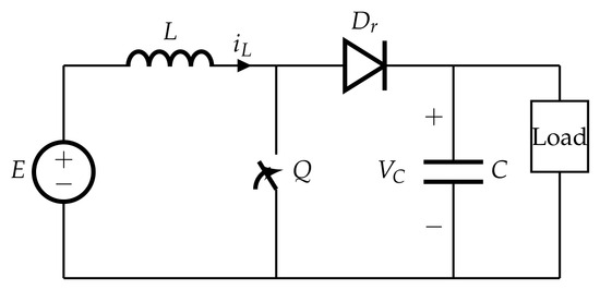
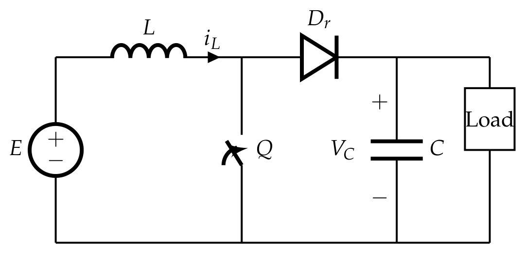
The DC–DC boost converter is used throughout this paper as the application case. Consider the circuit shown in Figure 1, which consists of an input voltage source E (provided by a PV panel), an inductor L with parasitic resistance $R_L$, a controlled switch (MOSFET), a diode, an output capacitor C, and a load (battery bank) at voltage $V_{\mathrm{bat}}$.

Figure 1. Schematic of the DC–DC boost converter.

2.6.1. Averaged Model

Under the continuous-conduction mode (CCM) assumption, the state-space averaged model of the boost converter is [37,38]

$$\begin{array}{cc}\hfill L{\displaystyle \frac{\mathrm{d}{i}_L}{\mathrm{d}t}}& =E-i_L{R}_L-V_C(1-D_C),\hfill \end{array}$$

(10)

$$\begin{array}{cc}\hfill C{\displaystyle \frac{\mathrm{d}{V}_C}{\mathrm{d}t}}& =i_L(1-D_C)-{\displaystyle \frac{V_C}{R_{\mathrm{bat}}}},\hfill \end{array}$$

(11)

where $i_L$ is the inductor current, $V_C$ is the capacitor voltage, $D_C\in [0,1]$ is the duty cycle (control input), and $R_{\mathrm{bat}}=V_{\mathrm{bat}}^2/P_{\mathrm{bat}}$ is the equivalent battery resistance.

2.6.2. Current-Loop Dynamics

For the current regulation loop, the inductor current Equation (10) can be written in the standard form

$${\displaystyle \frac{\mathrm{d}{i}_L}{\mathrm{d}t}}=\underset{a}{\underbrace{{\displaystyle \frac{E-V_C}{L}}}}+\underset{b}{\underbrace{{\displaystyle \frac{V_C}{L}}}}{D}_C,$$

(12)

where $a=(E-V_C)/L$ is the drift and $b=V_C/L$ is the control gain [39]. The drift a is negative in boost operation (since $V_C>E$), and its magnitude can be very large (order ${10}^5$ for typical PV systems). The control gain b is positive and depends on the output voltage $V_C$, which varies with the battery bank:

$$b_{\min }={\displaystyle \frac{V_{C,\min }}{L}},b_{\max }={\displaystyle \frac{V_{C,\max }}{L}}.$$

(13)

2.6.3. Gain Uncertainty

Defining nominal values $a_n=(E_n-V_{C,n})/L_n$ and $b_n=V_{C,n}/L_n$, the multiplicative gain uncertainty is

$$\Delta g={\displaystyle \frac{b}{b_n}}={\displaystyle \frac{V_C{L}_n}{V_{C,n}L}},$$

(14)

which varies as $V_C$ changes with the operating point. For a system serving battery banks from $V_{C,\min }$ to $V_{C,\max }$ with nominal voltage $V_{C,n}$, the uncertainty ratio is

$$\beta =\max \left({\displaystyle \frac{V_{C,\max }}{V_{C,n}}},{\displaystyle \frac{V_{C,n}}{V_{C,\min }}}\right).$$

(15)

2.6.4. Nominal Operating Point

At steady state, $\mathrm{d}{i}_L/\mathrm{d}t=0$ in (12), giving the nominal duty cycle

$$D_n=1-{\displaystyle \frac{E_n}{V_{C,n}}}.$$

(16)

2.6.5. Photovoltaic Source and MPPT

The input voltage E is provided by a PV panel whose current–voltage characteristic $I=I_{\mathrm{pv}}(V,G,T)$ depends on irradiance G and temperature T [40]. The maximum power point (MPP) varies with environmental conditions. An MPPT algorithm generates the current reference $i_{\mathrm{ref}}$ for the inner loop. In this work, an adaptive-step P&O algorithm is employed, where the perturbation step is modulated by the power derivative to achieve fast convergence near the MPP and reduced oscillation at steady state [23].

3. Control Design

3.1. System Class

Consider the class of uncertain nonlinear systems studied by Misawa [8]:

$$\dot{\mathbf{x}}=\widehat{\mathbf{f}}\left(\mathbf{x}\right)+\widehat{\mathbf{g}}\left(\mathbf{x}\right)\Delta gu+\Delta \mathbf{f}(·)+\mathbf{d}\left(t\right),$$

(17)

where $\mathbf{x}\in {\mathbb{R}}^n$ is the state, $u\in \mathbb{R}$ is the control input, $\widehat{\mathbf{f}}$ and $\widehat{\mathbf{g}}$ are the known nominal vector fields, $\Delta \mathbf{f}$ represents the unmatched additive uncertainty, $\mathbf{d}\left(t\right)$ is an external disturbance, and $\Delta g$ satisfies

$${\displaystyle \frac{1}{\beta }}\le \Delta g\le \beta ,\beta \ge 1.$$

(18)

The assumptions of [8] are retained; in particular, the sign condition $D\left[k\right]\widehat{\mathbf{g}}\left(\mathbf{x}\left[k\right]\right)>0$ is assumed to hold for all k.

Remark 3 ($\beta$ is a design parameter).

The bound $\beta \ge 1$ is known a priori from the operating range of the plant. The realized gain $\Delta g\in [1/\beta ,\beta ]$ is unknown and may vary in time.

3.2. Discrete-Time Plant Model

The forward-Euler discretization of (17) yields

$$\mathbf{x}[k+1]=\mathbf{x}\left[k\right]+T_s\left(\widehat{\mathbf{f}}\left[k\right]+\widehat{\mathbf{g}}\left[k\right]\Delta gu\left[k\right]+\Delta \mathbf{f}\left[k\right]+\mathbf{d}\left[k\right]\right).$$

(19)

Separating known and unknown components:

$$\mathbf{x}[k+1]=\mathbf{x}\left[k\right]+T_s(\underset{\mathrm{known}}{\underbrace{\widehat{\mathbf{f}}\left[k\right]+\widehat{\mathbf{g}}\left[k\right]u\left[k\right]}}+\underset{\mathrm{unknown}}{\underbrace{h\left[k\right]}}),$$

(20)

where $h\left[k\right]=\Delta \mathbf{f}\left[k\right]+\widehat{\mathbf{g}}\left[k\right](\Delta g-1)u\left[k\right]+\mathbf{d}\left[k\right]$.

Remark 4 (Sampling rate and drift compensation).

The controller operates at a sampling rate $f_s=40$ kHz, while the converter switches at $f_{\mathrm{sw}}=400$ kHz; each control update thus spans ten switching periods, over which the inductor current ripple is averaged. The forward-Euler model (19) describes the sample-to-sample dynamics at the controller rate and is well suited for control design on this time scale. However, the uncompensated open-loop map is expansive: with $T_s\left|a_n\right|\approx 2.27$ for the boost converter parameters of Section 4, the eigenvalue $|1+T_s{a}_n|\approx 1.27>1$, so the inductor current would diverge without active control. This is precisely the role of the nominal control $u_0$ and the ISM integrator z: they cancel the large drift $a_n$ from the σ-channel, making the compensated map contractive.

3.3. Sliding Variable

The sliding variable is $S\left[k\right]=S\left(\tilde{\mathbf{x}}\left[k\right]\right)$, where $\tilde{\mathbf{x}}=\mathbf{x}-{\mathbf{x}}_d$ is the tracking error. With gradient $D=\partial S/\partial \tilde{\mathbf{x}}$, the one-step evolution is

$$S[k+1]=S\left[k\right]+T_{s}f\left[k\right]+T_{s}g\left[k\right]\Delta gu\left[k\right]+T_s{P}_S\left[k\right],$$

(21)

where $f\left[k\right]=D\widehat{\mathbf{f}}\left[k\right]$, $g\left[k\right]=D\widehat{\mathbf{g}}\left[k\right]$, and $P_S\left[k\right]=D(\Delta \mathbf{f}\left[k\right]+\mathbf{d}\left[k\right])$.

3.4. Integral Sliding Mode Structure

Following the ISM framework introduced in Section 2, the control is decomposed as $u\left[k\right]=u_0\left[k\right]+u_1\left[k\right]$, and the auxiliary variable is

$$\sigma \left[k\right]=S\left[k\right]+z\left[k\right],z\left[0\right]=-S\left[0\right].$$

(22)

The integrator z is updated as

$$z[k+1]=z\left[k\right]-T_s\left(f\left[k\right]+g\left[k\right]u_0\left[k\right]\right),$$

(23)

yielding the $\sigma$-recursion

$$\sigma [k+1]=\sigma \left[k\right]+T_{s}g\left[k\right]\Delta g{u}_1\left[k\right]+T_{s}P\left[k\right],$$

(24)

where the aggregated perturbation is

$$P\left[k\right]=g\left[k\right](\Delta g-1)u_0\left[k\right]+P_S\left[k\right].$$

(25)

Remark 5 (Role of ISM).

The integrator (23) removes the nominal drift f and the nominal control effect $g{u}_0$ from the σ-channel, leaving only the perturbation P and the robust control $u_1$ in the recursion (24). Since $\sigma \left[0\right]=0$ by construction, the variable σ starts inside any boundary layer $\Psi =\left\{\right|\sigma |\le \varphi \}$ regardless of the initial condition of S, and the reaching phase is entirely bypassed.

3.5. Nominal Control

The nominal control provides the desired closed-loop dynamics in the absence of uncertainty. Setting $S[k+1]=(1-T_s{k}_0)S\left[k\right]$ in the nominal recursion yields

$$u_0\left[k\right]={\displaystyle \frac{1}{g\left[k\right]}}\left(-f\left[k\right]-k_{0}S\left[k\right]\right),$$

(26)

where $k_0>0$ satisfies $0<T_s{k}_0<2$. The first term cancels the nominal drift (feedforward), and the second drives the error to zero (proportional feedback).

Remark 6 (Practical relevance of the assumptions).

Three hypotheses underpin the stability analysis:

1.

Eingenvalue condition: the inequality $T_s{k}_0<2$ ensures that the nominal closed-loop eigenvalue $(1-T_s{k}_0)\in (-1,1)$, i.e., the discretized nominal dynamics are stable. For the boost converter of Section 4, $T_s{k}_0=25\times {10}^{-6}\times 5000=0.125$, well within the stability margin.

2.

Finite β: the uncertainty ratio $\beta =\sqrt{V_{C,\max }/V_{C,\min }}$ is determined by the physical operating range of the converter. For the three battery banks (24–72 V), $\beta =\sqrt{3}\approx 1.732$. This bound is known a priori from the system design and does not require online estimation. The optimal gain ${\theta }^{\star }$ depends explicitly on β; if β is underestimated, the contraction guarantee may be violated at the actual gain extremes, so conservative sizing is recommended.

3.

Lipschitz continuity of $\mathit{P}$: the aggregated perturbation $P\left[k\right]$ depends on the capacitor voltage $v_C$, the inductance L, and the input voltage E, all of which are continuous physical quantities with bounded rates of change (limited by the energy storage in C and L). The Lipschitz constant $L_P$ is therefore finite for any practical power converter and determines the improvement from $O\left(T_s\right)$ to $O\left(T_s^2\right)$ in the σ-band when the estimator is active.

3.6. Reduced $\sigma$-Iteration and Optimal Reaching Gain

With the robust control

$$u_1\left[k\right]=-{\displaystyle \frac{{\theta }_k\varphi }{T_{s}g\left[k\right]}}\mathrm{sat}\left({\displaystyle \frac{\sigma \left[k\right]}{\varphi }}\right),$$

(27)

the $\sigma$-dynamics inside the boundary layer $\left|\sigma \right|\le \varphi$ reduce to

$$\sigma [k+1]=(1-{\theta }_k\Delta g)\sigma \left[k\right]+T_{s}P\left[k\right].$$

(28)

3.6.1. A Family of Reaching Gains

The homogeneous part of (28) contracts the auxiliary variable by the worst-case one-step factor

$$J\left(\theta \right):=\underset{\Delta g\in [1/\beta ,\beta ]}{\max }\left|1-\theta \Delta g\right|,$$

(29)

so a reaching gain is characterized by the contraction it guarantees.

Definition 3 (Contraction profile).

A function $K:[1,\infty )\to [0,1)$ is a contraction profile if it is continuous and strictly increasing, with $K\left(1\right)=0$ and $K\left(\beta \right)\to 1$ as $\beta \to \infty$. The set of contraction profiles is denoted $\mathcal{R}$.

A profile encodes a guaranteed in-layer contraction $\left|\sigma [k+1]\right|\le K\left(\beta \right)\left|\sigma \left[k\right]\right|+T_s\left|P\left[k\right]\right|$ and hence an ultimate band proportional to $1/(1-K(\beta \left)\right)$. The subset of profiles that can be realized by an admissible reaching gain is denoted ${\mathcal{R}}^{\star }\subseteq \mathcal{R}$ (characterized in Proposition 1 below).

Example 1 (Two reaching gains yield different bands).

The exponential profile $K_1\left(\beta \right)=1-e^{-(\beta -1)}$ and the rational profile $K_2\left(\beta \right)=1-{\beta }^{-2}$ both belong to ${\mathcal{R}}^{\star }$ (since $K_1,K_2\ge r^{\star }$ for all $\beta \ge 1$). Their ultimate bands scale as $1/(1-K_1)=e^{\beta -1}$ and $1/(1-K_2)={\beta }^2$, respectively. Neither profile dominates the other across all β, which raises the question of which profile is best.

3.6.2. The Optimal Reaching Gain

Among all realizable profiles, the one that minimizes the ultimate band (equivalently, the worst-case contraction factor) is the optimal profile $K^{\star }=r^{\star }$, the lower boundary of ${\mathcal{R}}^{\star }$. This is a minimax result for the scalar one-step contraction inside the boundary layer, not a claim of global optimality of the complete controller. The corresponding gain solves

$${\theta }^{\star }=\arg \underset{\theta >0}{\min }J\left(\theta \right),$$

(30)

where $J\left(\theta \right)$ is defined in (29).

Lemma 1 (Optimal scalar contraction gain).

The problem (30) admits the unique solution

$${\theta }^{\star }={\displaystyle \frac{2\beta }{{\beta }^2+1}},$$

(31)

with optimal worst-case contraction factor $J\left({\theta }^{\star }\right)=r^{\star }\left(\beta \right)={\displaystyle \frac{{\beta }^2-1}{{\beta }^2+1}}$. Moreover, $r^{\star }\left(\beta \right)<1$ for every finite β (with $r^{\star }\left(1\right)=0$), and ${\theta }^{\star }\Delta g<2$ for all $\Delta g\in [1/\beta ,\beta ]$, so the in-layer map is nonexpansive.

Proof. 

For fixed $\theta >0$, the map $\Delta g\mapsto |1-\theta \Delta g|$ is convex, so its maximum over the compact interval $[1/\beta ,\beta ]$ is attained at an endpoint:

$$J\left(\theta \right)=\max \left\{|1-\theta /\beta |,|1-\theta \beta |\right\}.$$

(32)

On $(0,\beta )$ the first term is non-increasing in $\theta$, while on $(1/\beta ,\infty )$ the second is non-decreasing; since $\beta >1$, the two coincide at the unique $\theta$ satisfying $1-\theta /\beta =\theta \beta -1$, i.e., $\theta (\beta +1/\beta )=2$, which gives (31). For $\theta <{\theta }^{\star }$ the maximum in (32) equals the (larger) first term and exceeds its value at ${\theta }^{\star }$; for $\theta >{\theta }^{\star }$ it equals the second and likewise exceeds it. Hence ${\theta }^{\star }$ is the unique minimizer of J (equioscillation):

$$J\left({\theta }^{\star }\right)=\left|1-{\displaystyle \frac{2{\beta }^2}{{\beta }^2+1}}\right|={\displaystyle \frac{{\beta }^2-1}{{\beta }^2+1}}=:r^{\star }.$$

(33)

Finally, ${\theta }^{\star }\beta =2{\beta }^2/({\beta }^2+1)<2$, so $|1-{\theta }^{\star }\Delta g|\le r^{\star }<1$ for every $\Delta g\in [1/\beta ,\beta ]$ and finite $\beta$, with $r^{\star }\left(1\right)=0$.    □

Proposition 1 (Realizability floor).

A contraction profile $K\in \mathcal{R}$ is realizable if and only if $K\left(\beta \right)\ge r^{\star }\left(\beta \right)$ for all β: no reaching gain attains a worst-case factor below $r^{\star }$.

Proof. 

By Lemma 1, $r^{\star }\left(\beta \right)={\min }_{\theta }J\left(\theta \right)$, so no factor below $r^{\star }$ is attainable. Conversely, for any $c\in [r^{\star }\left(\beta \right),1)$, taking $\theta =(c+1)/\beta$ yields $J\left(\theta \right)=c$.    □

In practical terms, the improvement from the optimal gain is most significant at moderate uncertainty ratios (e.g., $\beta =\sqrt{3}$ gives $r^{\star }=0.5$, halving the sliding variable per step), while for very large $\beta$ the contraction approaches unity and additional mechanisms (gain scheduling, online estimation of $\beta$) would be needed.

The complete reaching law is

$${\theta }_k^{\star }=\left\{\begin{array}{cc}{\displaystyle \frac{2\beta }{{\beta }^2+1}},\hfill & \left|\sigma \right[k\left]\right|\le \varphi ,\hfill \\ \min \left({\displaystyle \frac{\left|\sigma \right[k\left]\right|\beta }{\varphi }},{\displaystyle \frac{2}{\beta }}\right),\hfill & \left|\sigma \right[k\left]\right|>\varphi .\hfill \end{array}\right.$$

(34)

The two-branch structure of (34) serves complementary objectives: the inside branch applies the optimal ${\theta }^{\star }$ for worst-case contraction within the band, while the outside branch provides monotone convergence toward $\Psi$.

Outside the boundary layer ($\left|\sigma \right[k\left]\right|>\varphi$), $\mathrm{sat}(\sigma /\varphi )=\mathrm{sign}\left(\sigma \right)$ and the $\sigma$-dynamics reduce to $\sigma [k+1]=\sigma \left[k\right]-{\theta }_k\Delta g\varphi \mathrm{sign}\left(\sigma \left[k\right]\right)+T_{s}P\left[k\right]$. The two limits in the outside branch of (34) serve complementary purposes: the linear term $\left|\sigma \right[k\left]\right|\beta /\varphi$ provides one-step reaching to the origin under the minimum gain $\Delta g=1/\beta$, while the cap $2/\beta$ prevents the trajectory from overshooting past $-\varphi$ under the maximum gain $\Delta g=\beta$. Specifically, for $\sigma >0$ and $\Delta g=\beta$, the no-overshoot condition $\sigma [k+1]\ge -\varphi$ requires ${\theta }_k\le (\sigma +\varphi )/\left(\beta \varphi \right)$, which at the boundary $\sigma =\varphi$ yields ${\theta }_k\le 2/\beta$. The minimum of both limits selects the most conservative gain at each step, ensuring monotone convergence toward $\Psi$ for every $\Delta g\in [1/\beta ,\beta ]$.

Once the ISM is activated at $k_a$ with $\sigma \left[k_a\right]=0$, the trajectory starts inside $\Psi$ and the in-band invariance condition $T_s{P}_{\mathrm{eff},\max }\le (1-r^{\star })\varphi ={\displaystyle \frac{2}{{\beta }^2+1}}\varphi$ guarantees that $\sigma$ never leaves the boundary layer. Consequently, the outside branch of (34) is inactive for all $k\ge k_a$ and governs only a possible pre-activation transient.

Remark 7 (Connection to relaxation theory).

Under the identification $[m,M]=[1/\beta ,\beta ]$, the optimal reaching gain ${\theta }^{\star }=2/(m+M)$ and the contraction factor $r^{\star }=(\kappa -1)/(\kappa +1)$ with $\kappa ={\beta }^2$ coincide with the optimal stationary relaxation parameter of Definition 1. The worst-case optimization framing traces back to Richardson [41], with the closed-form solution due to [35]; equivalently, ${\theta }^{\star }$ is Nesterov’s first-order step $2/(L+\mu )$ with $\kappa =L/\mu$ [36]. The present Lemma transposes this classical result from numerical linear algebra to the discrete-time sliding-variable iteration under multiplicative gain uncertainty. As shown in Remark 2, the fixed-gain design of [8] ceases to contract for $\beta \ge 3/2$; in contrast, $r^{\star }\left(\beta \right)<1$ for every finite β. Notably, ${\theta }^{\star }\le 1$ for all $\beta >1$: the worst-case-optimal gain is a sub-unity under-relaxation, whereas the fixed gain $(\eta +2\epsilon )/(\eta +\epsilon )\in (1,2)$ over-relaxes.

3.7. Disturbance Estimation

To further reduce the quasi-sliding band, a past-step disturbance estimation is incorporated. The estimator reconstructs $P[k-1]$ (not the current $P\left[k\right]$) and is therefore effective when the perturbation varies slowly relative to the sampling period, i.e., $\left|P\right[k]-P[k-1\left]\right|\ll \left|P\right[k\left]\right|$. In power converters this condition is satisfied because the dominant perturbation sources ($v_C$, L, E) have time constants much larger than $T_s$; for fast-changing disturbances, additional prediction or filtering would be required. From (24), the perturbation at the previous step satisfies

$$P[k-1]={\displaystyle \frac{\sigma \left[k\right]-\sigma [k-1]}{T_s}}-g[k-1]\Delta g{u}_1[k-1].$$

(35)

Since $\Delta g$ is unknown, the estimate uses the nominal gain:

$$\widehat{P}[k-1]={\displaystyle \frac{\sigma \left[k\right]-\sigma [k-1]}{T_s}}-g[k-1]u_1[k-1].$$

(36)

At the first step after activation, $\widehat{P}$ is initialized to zero. The estimation error is

$$\widehat{P}[k-1]-P[k-1]=g[k-1](\Delta g-1)u_1[k-1],$$

(37)

which vanishes when $\Delta g=1$ and grows with $|\Delta g-1|$.

The robust control with disturbance compensation becomes

$$u_1\left[k\right]=-{\displaystyle \frac{{\theta }_k^{\star }\varphi }{T_{s}g\left[k\right]}}\mathrm{sat}\left({\displaystyle \frac{\sigma \left[k\right]}{\varphi }}\right)-{\displaystyle \frac{{\alpha }_{\mathrm{est}}\widehat{P}[k-1]}{g\left[k\right]}},$$

(38)

where ${\alpha }_{\mathrm{est}}\in (0,1]$ is a confidence factor. Selecting ${\alpha }_{\mathrm{est}}=1/\beta$ ensures

$${\alpha }_{\mathrm{est}}(\beta -1)={\displaystyle \frac{\beta -1}{\beta }}<1,$$

(39)

which attenuates the estimation-error contribution, since $\Delta g{\alpha }_{\mathrm{est}}\le (\beta -1)/\beta <1$, preventing destabilization.

Effect on the $\sigma$-Dynamics

Substituting (38) into (24), the effective perturbation becomes $P_{\mathrm{eff}}\left[k\right]=P\left[k\right]-\Delta g{\alpha }_{\mathrm{est}}\widehat{P}[k-1]$, which decomposes as

$$\begin{array}{cc}\hfill P_{\mathrm{eff}}\left[k\right]& =\underset{\mathrm{Lipschitz}\mathrm{residual}}{\underbrace{\left(P\left[k\right]-P[k-1]\right)}}+\underset{\mathrm{gain}\mathrm{mismatch}}{\underbrace{\left(1-\Delta g{\alpha }_{\mathrm{est}}\right)P[k-1]}}\hfill \\ \hfill & -\underset{\mathrm{estimation}\mathrm{error}}{\underbrace{\Delta g{\alpha }_{\mathrm{est}}{e}_P[k-1]}},\hfill \end{array}$$

(40)

where $e_P=\widehat{P}-P$. A rigorous bound follows from the triangle inequality:

$$|P_{\mathrm{eff}}\left[k\right]|\le (1-{\alpha }_{\mathrm{est}}\Delta g)|P\left[k\right]|+{\alpha }_{\mathrm{est}}\Delta g|P\left[k\right]-P[k-1]|.$$

(41)

The first term is the gain-mismatch residual; the second is the Lipschitz residual $|P\left[k\right]-P[k-1]|\le L_P{T}_s$. Therefore:

$$P_{\mathrm{eff},\max }\le (1-{\alpha }_{\mathrm{est}}\Delta g)P_{\max }+{\alpha }_{\mathrm{est}}\Delta g{L}_P{T}_s.$$

(42)

when ${\alpha }_{\mathrm{est}}\Delta g=1$ (nominal gain), the first term vanishes and $P_{\mathrm{eff},\max }=L_P{T}_s=O\left(T_s\right)$, yielding the $O\left(T_s^2\right)$ band. At the gain extremes ($\Delta g=1/\beta$ or $\Delta g=\beta$), the first term dominates and the band remains $O\left(T_s\right)$. The boundary layer $\varphi$ must be sized using (42) rather than $P_{\max }$ alone when the estimator is active.

3.8. Boundary Layer Design

The boundary-layer thickness satisfies

$$\varphi \ge {\displaystyle \frac{T_s{P}_{\max }({\beta }^2+1)}{2}},$$

(43)

and is sized as

$$\varphi ={\displaystyle \frac{T_s}{2}}\left((1+{\beta }^2)\eta +2{\beta }^2\epsilon \right),$$

(44)

where $\eta \ge P_{\max }$ and $\epsilon >0$ is a design margin.

3.9. Anti-Windup

When the control saturates, the integrator z is frozen to prevent error accumulation:

$$z[k+1]=\left\{\begin{array}{cc}z\left[k\right]-T_s\left(f\left[k\right]+g\left[k\right]u_0\left[k\right]\right),\hfill & u_{\min }<u\left[k\right]<u_{\max },\hfill \\ z\left[k\right],\hfill & \mathrm{otherwise},\hfill \end{array}\right.$$

(45)

where $u_{\min }$ and $u_{\max }$ are the physical actuator limits (for a power converter, $u_{\min }=0$ and $u_{\max }=1$).

3.10. Complete Control Law

The complete control is

$$u\left[k\right]=\underset{u_0\left[k\right]}{\underbrace{{\displaystyle \frac{1}{g\left[k\right]}}\left(-f\left[k\right]-k_{0}S\left[k\right]\right)}}+\underset{u_1\left[k\right]}{\underbrace{\left(-{\displaystyle \frac{{\theta }_k^{\star }\varphi }{T_{s}g\left[k\right]}}\mathrm{sat}\left({\displaystyle \frac{\sigma \left[k\right]}{\varphi }}\right)-{\displaystyle \frac{{\alpha }_{\mathrm{est}}\widehat{P}[k-1]}{g\left[k\right]}}\right)}},$$

(46)

where ${\theta }_k^{\star }$ is given by (34), $\widehat{P}$ by (36) (with $\widehat{P}[k_a-1]=0$), $\varphi$ by (44), and $\sigma =S+z$ with z updated by (23)–(45).

3.11. Stability Analysis

Theorem 1 (Convergence under ISM with optimal reaching and estimation).

Consider the system (17), with the control (46), activated at the instant $k_a\ge 0$ at which the ISM is initialized with $z\left[k_a\right]=-S\left[k_a\right]$. Suppose $k_0>0$, $T_s{k}_0<2$, $\Delta g\in [1/\beta ,\beta ]$, ${\alpha }_{\mathrm{est}}=1/\beta$, ϕ satisfies (43), and P is Lipschitz along trajectories, i.e., $|P\left[k\right]-P[k-1]|\le L_P{T}_s$ for some $L_P>0$. Then:

(i) 

No reaching phase: $\sigma \left[k_a\right]=0\in \Psi$.

(ii) 

$\mathit{\sigma }$-invariance: For all $k\ge k_a$,

$$\left|\sigma [k+1]\right|\le r^{\star }\left(\beta \right)\left|\sigma \left[k\right]\right|+T_s\left|P_{\mathrm{eff}}\left[k\right]\right|.$$

(47)

(iii) 

$\mathit{\sigma }$ ultimate bound:

$$\underset{k\to \infty }{\lim \sup }\left|\sigma \left[k\right]\right|\le {\displaystyle \frac{T_s{P}_{\mathrm{eff},\max }({\beta }^2+1)}{2}},$$

(48)

where $P_{\mathrm{eff},\max }\le P_{\max }$. Under Lipschitz continuity on P and $\Delta g\approx 1$, $P_{\mathrm{eff},\max }=O\left(T_s\right)$, yielding ${\left|\sigma \right|}_{\mathrm{ss}}=O\left(T_s^2\right)$.

(iv) 

Robust contraction: $r^{\star }\left(\beta \right)<1$ for every finite β.

(v) 

State convergence:

$$\left|S\left[k\right]\right|\le {(1-T_s{k}_0)}^{k-k_a}\left|S\left[k_a\right]\right|+O\left(T_s\right).$$

(49)

Proof. 

Consider $V\left[k\right]={\sigma }^2\left[k\right]$.

(i) 

By construction, $\sigma \left[k_a\right]=S\left[k_a\right]+z\left[k_a\right]=0$.

(ii) 

Inside $\Psi$, $\mathrm{sat}(\sigma /\varphi )=\sigma /\varphi$, so (24) with the robust control (27) gives $\sigma [k+1]=(1-{\theta }^{\star }\Delta g)\sigma \left[k\right]+T_s{P}_{\mathrm{eff}}\left[k\right]$. Taking absolute values:

$$\left|\sigma [k+1]\right|\le |1-{\theta }^{\star }\Delta g\left|\right|\sigma \left[k\right]|+T_s\left|P_{\mathrm{eff}}\left[k\right]\right|.$$

(50)

By Lemma 1, $|1-{\theta }^{\star }\Delta g|\le r^{\star }\left(\beta \right)$ for all $\Delta g\in [1/\beta ,\beta ]$, yielding (47). For the Lyapunov function $V\left[k\right]={\sigma }^2\left[k\right]$:

$$\begin{array}{cc}\hfill V[k+1]& ={\left[(1-{\theta }^{\star }\Delta g)\sigma \left[k\right]+T_s{P}_{\mathrm{eff}}\left[k\right]\right]}^2\hfill \\ \hfill & \le {\left(r^{\star }\left|\sigma \left[k\right]\right|+T_s{P}_{\mathrm{eff},\max }\right)}^2\hfill \\ \hfill & ={\left[r^{\star }\right]}^{2}V\left[k\right]+2r^{\star }\left|\sigma \left[k\right]\right|T_s{P}_{\mathrm{eff},\max }+T_s^2{P}_{\mathrm{eff},\max }^2.\hfill \end{array}$$

(51)

Since $\left|\sigma \right[k\left]\right|\le \varphi$ inside $\Psi$ and ${\left[r^{\star }\right]}^2<1$, this is a geometric contraction with an additive perturbation term of order $O\left(T_s\right)$. The no-overshoot condition ${\theta }^{\star }\beta =2{\beta }^2/({\beta }^2+1)<2$ holds for all finite $\beta$, so the trajectory cannot jump past the opposite boundary of $\Psi$.

(iii) 

The recursion $\left|\sigma [k+1]\right|\le r^{\star }\left|\sigma \left[k\right]\right|+T_s{P}_{\mathrm{eff},\max }$ is a contractive iteration with additive input. Its fixed point ${\left|\sigma \right|}_{\infty }$ satisfies ${\left|\sigma \right|}_{\infty }=r^{\star }{\left|\sigma \right|}_{\infty }+T_s{P}_{\mathrm{eff},\max }$, yielding

$${\left|\sigma \right|}_{\infty }={\displaystyle \frac{T_s{P}_{\mathrm{eff},\max }}{1-r^{\star }}}={\displaystyle \frac{T_s{P}_{\mathrm{eff},\max }({\beta }^2+1)}{2}},$$

(52)

where $1-r^{\star }=2/({\beta }^2+1)$ was used. This establishes (48). Under Lipschitz continuity on P and $\Delta g=1$: $P_{\mathrm{eff},\max }\le L_P{T}_s$ from (40), so ${\left|\sigma \right|}_{\mathrm{ss}}=O\left(T_s^2\right)$.

(iv) 

$r^{\star }\left(\beta \right)=({\beta }^2-1)/({\beta }^2+1)<1$ since ${\beta }^2-1<{\beta }^2+1$.

(v) 

From $S=\sigma -z$, the z-update (23), and the $\sigma$-recursion (24), the S-dynamics satisfy

$$S[k+1]=(1-T_s{k}_0)S\left[k\right]+\left(\sigma [k+1]-\sigma \left[k\right]\right).$$

(53)

Inside the band, the $\sigma$-increment is $\sigma [k+1]-\sigma \left[k\right]=-{\theta }^{\star }\Delta g\sigma \left[k\right]+T_s{P}_{\mathrm{eff}}\left[k\right]$. Once $\sigma$ has converged to its ultimate bound, the successive differences satisfy $|\sigma [k+1]-\sigma \left[k\right]|\le r^{\star }|\sigma \left[k\right]-\sigma [k-1]|+T_s|P_{\mathrm{eff}}\left[k\right]-P_{\mathrm{eff}}[k-1]|$, which, under the Lipschitz hypothesis, yields $|\sigma [k+1]-\sigma \left[k\right]|=O\left(T_s^2\right)$ in steady state. Defining $r_e\left[k\right]=(\sigma [k+1]-\sigma \left[k\right])/T_s$, one obtains $|r_e|=O\left(T_s\right)$, and the geometric factor $(1-T_s{k}_0)$ with $0<T_s{k}_0<2$ gives (49).    □

Remark 8 (Ideal case: absence of perturbation).

In the nominal case $P\equiv 0$ and $\Delta g=1$, the ISM variable satisfies $\sigma \left[k\right]\equiv 0$ for all $k\ge k_a$ (since $\sigma \left[k_a\right]=0$ and the recursion (28) reduces to $\sigma [k+1]=(1-{\theta }^{\star })\sigma \left[k\right]$), and the sliding variable converges as $S\left[k\right]={(1-T_s{k}_0)}^{k-k_a}S\left[k_a\right]\to 0$. That is, in the absence of uncertainty and disturbance, both σ and S reach zero exactly—σ instantaneously by ISM construction, and S geometrically by the nominal control $u_0$. The nonzero values observed in practice are entirely attributable to the perturbation P and the gain mismatch $\Delta g\ne 1$.

Remark 9 (Convergence orders of S and $\sigma$).

The state S converges to $O\left(T_s\right)$ due to the integral action of z. The variable σ converges to a band determined by $P_{\mathrm{eff}}$ and $r^{\star }$, with a further tightening when estimation is active, as quantified in Theorem 1(iii). The estimation improves only the σ-band; the S convergence order is unchanged.

Remark 10 (Complementary operating regimes).

The optimal reaching gain and the disturbance estimator address complementary regimes of the gain uncertainty. At the voltage extremes ($V_C=24$ or 72 V), $\Delta g$ deviates significantly from unity and the estimation error $\left(\Delta g-1\right)u_1$ is large; here, the optimal gain ${\theta }^{\star }$ is essential to guarantee contraction ($r^{\star }<1$), while the estimator provides only a modest reduction of the σ-band. Near the nominal voltage ($V_C\approx V_{C,n}$), $\Delta g\approx 1$ and the estimation error vanishes; here, the estimator tightens the σ-band effectively, while ${\theta }^{\star }$ is less critical since any reasonable θ would contract. Together, the two mechanisms provide robust performance across the entire operating range.

4. Application: Photovoltaic Battery Charging System

This section specializes the ISM controller with optimal reaching gain and disturbance estimation developed in Section 3 to a solar-powered battery charging system based on a DC–DC boost converter.

4.1. System Overview

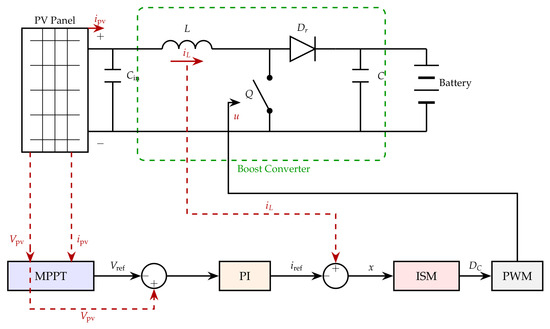
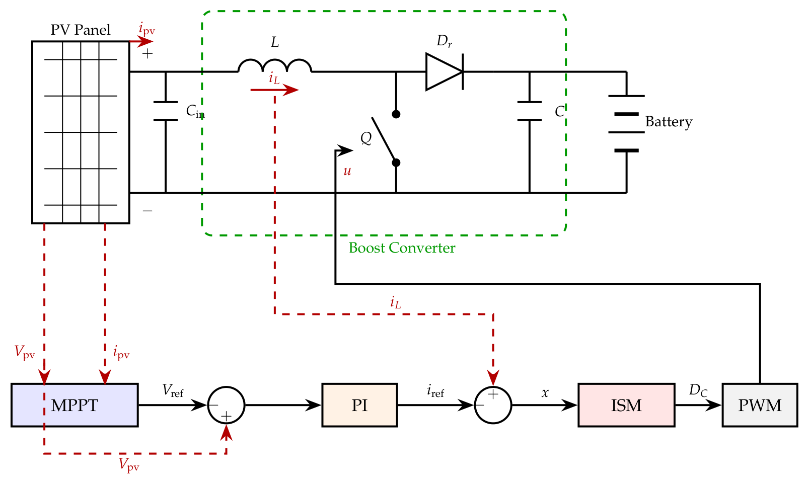
The system consists of a PV panel connected to a battery bank through a DC–DC boost converter, as shown in Figure 2. The control architecture comprises two hierarchical layers: an outer MPPT loop that determines the optimal operating voltage $V_{\mathrm{ref}}$ (converted to a current reference $i_{\mathrm{ref}}$ by a proportional-integral (PI) controller), and an inner current regulation loop that tracks this reference by adjusting $D_C$ at the switching frequency $f_{\mathrm{sw}}$.

Figure 2. Schematic of the proposed PV-fed boost converter with battery load and control system. The power stage consists of the PV panel, input filter capacitor $C_{\mathrm{in}}$, boost converter (L, Q, $D_r$, C), and battery. The control chain (bottom) comprises the adaptive P&O MPPT, PI voltage-to-current converter, and ISM controller with optimal reaching gain. Dashed red lines indicate sensor signals.

The system is designed to charge battery banks of 24, 48, and 72 V using a single PV panel. Table 1 and Table 2 summarize the PV panel and converter parameters, respectively.

Table 1. PV panel parameters (SUNERGY SYM 90).

Parameter	Symbol	Value
Rated power at MPP	$P_{\mathrm{mp}}$	90 W
Voltage at MPP	$V_{\mathrm{mp}}$	18.37 V
Current at MPP	$I_{\mathrm{mp}}$	4.90 A
Open-circuit voltage	$V_{\mathrm{oc}}$	22.05 V
Short-circuit current	$I_{\mathrm{sc}}$	5.29 A

Table 2. Boost converter parameters.

Parameter	Symbol	Value
Inductance	L	255.81 $\mathsf{\mu }$H
Parasitic resistance of the inductor	$R_L$	0.32 $\Omega$
Output capacitance	C	998 $\mathsf{\mu }$F
Parasitic resistance of the capacitor	$R_C$	0.041 $\Omega$
Switching frequency	$f_{\mathrm{sw}}$	400 kHz
Battery bank voltages	$V_{\mathrm{bat}}$	24, 48, 72 V

4.2. MPPT Algorithm

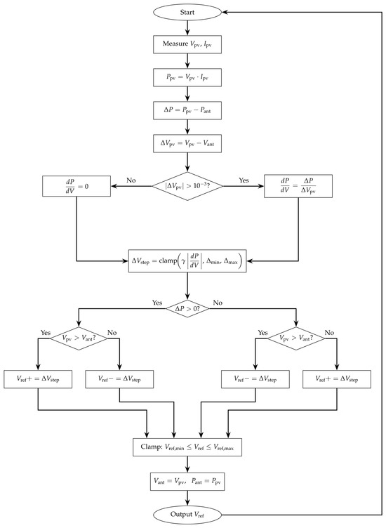
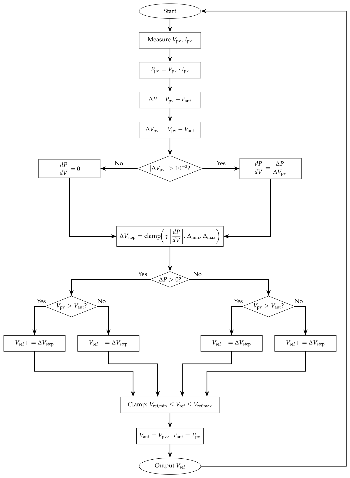
The MPPT is performed by an adaptive-step P&O algorithm [23,42]. The algorithm operates at a rate slower than the inner current loop (typically every $N_{\mathrm{mppt}}$ switching periods) and generates the voltage reference $V_{\mathrm{ref}}$ for the outer PI loop.

At each MPPT iteration, the PV power $P_{\mathrm{pv}}=V_{\mathrm{pv}}{I}_{\mathrm{pv}}$ is measured and compared with the previous value. The adaptive step size is computed as

$$\Delta V_{\mathrm{step}}=\mathrm{clamp}\left(\gamma \left|{\displaystyle \frac{dP}{dV}}\right|,{\Delta }_{\min },{\Delta }_{\max }\right),$$

(54)

where $\gamma >0$ is a scaling factor, ${\Delta }_{\min }$ and ${\Delta }_{\max }$ are the minimum and maximum perturbation sizes, and $\mathrm{clamp}(x,a,b)=\max (a,\min (b,x\left)\right)$. Near the MPP, $|dP/dV|\approx 0$ and the step reduces to ${\Delta }_{\min }$, suppressing steady-state oscillations. Far from the MPP, the large $|dP/dV|$ saturates the step at ${\Delta }_{\max }$, ensuring fast convergence. The perturbation direction (increase or decrease $V_{\mathrm{ref}}$) is determined by the standard P&O decision logic, as shown in the flowchart of Figure 3.

Figure 3. Flowchart of the adaptive-step P&O MPPT algorithm.

4.3. Controller Specialization for the Boost Converter

The general ISM controller (46) is now specialized to the boost converter current loop described in Section 2.6. The boost converter (12) is an instance of (17) with the identifications listed in Table 3.

Table 3. Identification of the boost converter with the general framework.

General	Boost Converter	Expression	Value
State x	$i_L$	—	Inductor current
Reference $x_d$	$i_{\mathrm{ref}}$	—	MPPT reference
Sliding surface S	$i_L-i_{\mathrm{ref}}$	—	Current error
Drift f	$a_n$	$(E_n-V_{C,n})/L_n$	$-\mathrm{90,690}$ s−1
Gain g	$b_n$	$V_{C,n}/L_n$	$\mathrm{162,505}$ s−1
Uncertainty $\Delta g$	$V_C{L}_n/\left(V_{C,n}L\right)$	—	$\in [1/\beta ,\beta ]$
Control u	$D_C$	—	Duty cycle $\in [0,1]$

4.3.1. Sliding Variable and ISM Initialization

The sliding variable is $S\left[k\right]=i_L\left[k\right]-i_{\mathrm{ref}}\left[k\right]$, with gradient $D=\partial S/\partial \tilde{x}=1$. The ISM auxiliary variable and integrator are

$$\begin{array}{cc}\hfill \sigma \left[k\right]& =S\left[k\right]+z\left[k\right],z\left[k_a\right]=-S\left[k_a\right],\hfill \end{array}$$

(55)

$$\begin{array}{cc}\hfill z[k+1]& =z\left[k\right]-T_s\left(a_n+b_n{u}_0\left[k\right]\right).\hfill \end{array}$$

(56)

The activation instant $k_a$ corresponds to the time at which the inductor current enters a neighborhood of the reference: $|i_L\left[k_a\right]-i_{\mathrm{ref}}|<x_{\mathrm{th}}$. Prior to activation, the converter operates with $D_n$ and the integrator is held at $z=-S$ to maintain $\sigma =0$.

4.3.2. Nominal Control

From (26), the nominal control law is given by

$$u_0\left[k\right]=\left(1-{\displaystyle \frac{E_n}{V_{C,n}}}\right)-{\displaystyle \frac{L_n{k}_0}{V_{C,n}}}S\left[k\right].$$

(57)

The first term corresponds to the feedforward duty cycle $D_n$, while the second term is a proportional correction that drives the current error to zero with rate $k_0$.

4.3.3. Robust Control with Optimal Reaching and Estimation

The robust control (38) specializes to

$$u_1\left[k\right]=-{\displaystyle \frac{{\theta }_k^{\star }\varphi }{T_s{b}_n}}\mathrm{sat}\left({\displaystyle \frac{\sigma \left[k\right]}{\varphi }}\right)-{\displaystyle \frac{{\alpha }_{\mathrm{est}}\widehat{P}[k-1]}{b_n}},$$

(58)

where ${\theta }_k^{\star }$ is given by (34) and the disturbance estimate is

$$\widehat{P}[k-1]={\displaystyle \frac{\sigma \left[k\right]-\sigma [k-1]}{T_s}}-b_n{u}_1[k-1],$$

(59)

with $\widehat{P}[k_a-1]=0$ at the first step after activation.

4.3.4. Complete Duty Cycle

The total $D_C$ applied to the converter is

$$D_C\left[k\right]={\mathrm{sat}}_{[0,1]}\left(u_0\left[k\right]+u_1\left[k\right]\right),$$

(60)

where ${\mathrm{sat}}_{[0,1]}$ enforces the physical duty-cycle constraint. The anti-windup mechanism (45) freezes the integrator z whenever $D_C$ saturates at 0 or 1.

4.4. Gain Uncertainty and Boundary Layer

4.4.1. Uncertainty Ratio

The multiplicative gain uncertainty (14) depends on the capacitor voltage $V_C$. To minimize the uncertainty ratio across all battery banks, the nominal capacitor voltage is selected as the geometric mean of the extreme battery voltages:

$$V_{C,n}=\sqrt{V_{C,\min }·V_{C,\max }},$$

(61)

which equalizes the uncertainty at both endpoints and yields

$$\beta =\sqrt{{\displaystyle \frac{V_{C,\max }}{V_{C,\min }}}}.$$

(62)

The corresponding optimal reaching parameters follow from Lemma 1:

$${\theta }^{\star }={\displaystyle \frac{2\beta }{{\beta }^2+1}},r^{\star }={\displaystyle \frac{{\beta }^2-1}{{\beta }^2+1}},{\alpha }_{\mathrm{est}}={\displaystyle \frac{1}{\beta }}.$$

(63)

4.4.2. Perturbation Bound

The aggregated perturbation in the $\sigma$-channel (25) for the boost converter is

$$P\left[k\right]=b_n(\Delta g-1)u_0\left[k\right]+P_S\left[k\right],$$

(64)

where $P_S$ accounts for the parasitic losses, inductance variation, and external disturbances. At steady state, $u_0\approx D_n$ and $|\Delta g-1|\le (\beta -1)$. Since $b_n{D}_n=\left|a_n\right|$, the gain-mismatch contribution simplifies to $|a_n|(\beta -1)$. The parasitic contribution is bounded by $P_{S,\max }\approx I_{\mathrm{sc}}{R}_{\mathrm{total}}/L$, where $R_{\mathrm{total}}=R_L+R_C+R_{\mathrm{DS},\mathrm{on}}+R_D\approx 1.0\Omega$ collects all conduction resistances in the power stage ($R_{\mathrm{DS},\mathrm{on}}$: MOSFET on-resistance, $R_D$: diode equivalent resistance), giving

$$P_{\max }\le \left|a_n\right|(\beta -1)+P_{S,\max }.$$

(65)

4.4.3. Boundary Layer

The boundary layer (44) with $\eta =P_{\max }$ and $\epsilon =0.2P_{\max }$ gives

$$\varphi ={\displaystyle \frac{T_s}{2}}\left((1+{\beta }^2)P_{\max }+2{\beta }^2·0.2P_{\max }\right)={\displaystyle \frac{T_s{P}_{\max }}{2}}\left(1+1.4{\beta }^2\right).$$

(66)

Remark 11 (Practical $\sigma$-band versus design $\varphi$).

The boundary layer (43) holds by construction: ϕ is computed offline from the known bounds $P_{\max }$, β, and $T_s$, all of which are determined at design time from the converter parameters and the operating range. No online verification is required. The layer is designed for the worst case ($\Delta g=\beta$, maximum parasitic perturbation). In practice, when the converter operates near the nominal voltage ($V_C\approx V_{C,n}$), $\Delta g\approx 1$ and the perturbation is dominated by the parasitic losses ($P\approx P_S\ll P_{\max }$). The actual σ-band is therefore much smaller than ϕ; simulations in Section 5 confirm that σ typically occupies less than 10% of the design boundary layer during near-nominal ($V_C\approx V_{C,n}$) operation; at the 24 V extreme, $|{\sigma }_{\mathrm{ss}}|$ reaches approximately 50% of ϕ by design.

4.5. Convergence Analysis for the Boost Converter

The following corollary specializes Theorem 1 to the boost converter.

Corollary 1 (Boost converter current regulation).

Consider the boost converter (12) with duty cycle (60), under the hypotheses of Theorem 1, activated at $k_a$ with $z\left[k_a\right]=-S\left[k_a\right]$. Suppose $V_C\in [V_{C,\min },V_{C,\max }]$. Then:

(i) 

The ISM variable σ starts at zero and remains in the band $\left|\sigma \right|\le \varphi$ for all $k\ge k_a$.

(ii) 

Inside the band, σ contracts with factor $r^{\star }\left(\beta \right)<1$ per step. At $\beta =\sqrt{3}$: $r^{\star }=0.5$.

(iii) 

The inductor current error converges geometrically:

$$|i_L\left[k\right]-i_{\mathrm{ref}}|\le {(1-T_s{k}_0)}^{k-k_a}|i_L\left[k_a\right]-i_{\mathrm{ref}}|+O\left(T_s\right).$$

(67)

with $k_0=5000$ s⁻¹ and $T_s=25\mu$s: ${\rho }_0=1-0.125=0.875$, giving a time constant $\tau =-T_s/\ln \left({\rho }_0\right)\approx 187\mu$s (approximately 7.5 sampling periods).

(iv) 

The σ-ultimate bound satisfies

$${\left|\sigma \right|}_{\mathrm{ss}}\le {\displaystyle \frac{T_s{P}_{\mathrm{eff},\max }({\beta }^2+1)}{2}}.$$

(68)

without estimation: ${\left|\sigma \right|}_{\mathrm{ss}}=O\left(T_s\right)$. With estimation and $\Delta g\approx 1$: ${\left|\sigma \right|}_{\mathrm{ss}}=O\left(T_s^2\right)$.

(v) 

The steady-state offset of σ is determined by the total perturbation at the operating point:

$${\sigma }_{\mathrm{ss}}\approx {\displaystyle \frac{T_s{P}_{\mathrm{ss}}}{{\theta }^{\star }\Delta g}},P_{\mathrm{ss}}=b_n(\Delta g-1)D_n-{\displaystyle \frac{i_{\mathrm{ref}}{R}_{\mathrm{total}}}{L}},$$

(69)

where the first term is the gain-mismatch contribution and the second collects the parasitic conduction losses. Near the nominal voltage ($\Delta g\approx 1$), the mismatch vanishes and ${\sigma }_{\mathrm{ss}}$ is dominated by the parasitic term; at the voltage extremes (e.g., $V_{\mathrm{bat}}=24$ V, $\Delta g=0.577$), the mismatch dominates and $|{\sigma }_{\mathrm{ss}}|$ reaches approximately 2.87 A. This offset is quasi-static, varying only when $i_{\mathrm{ref}}$ or $V_C$ change.

(vi) 

The steady-state bound on S combines the discretization residual and the switching ripple:

$${\left|S\right|}_{\mathrm{ss}}\le {\displaystyle \frac{T_s{\left|r_e\right|}_{\max }}{k_0}}+{\displaystyle \frac{E{D}_{\max }}{2L{f}_{\mathrm{sw}}}},$$

(70)

where $D_{\max }=1-E_n/V_{C,\max }$ is the highest duty cycle and $|r_e{|}_{\max }={|\sigma [k+1]-\sigma \left[k\right]|}_{\max }/T_s$. The first term is the one-step residual that the integrator z has not yet compensated; the second is the inductor current ripple due to PWM switching.

Proof. 

Properties (i)–(iv) follow directly from Theorem 1 with $f=a_n$, $g=b_n$, and $\Delta g=V_C{L}_n/\left(V_{C,n}L\right)$.

For (v), in steady state, the perturbation is $P_{\mathrm{ss}}=b_n(\Delta g-1)D_n-i_{\mathrm{ref}}{R}_{\mathrm{total}}/L$, which is approximately constant when $i_L\approx i_{\mathrm{ref}}$ and $V_C\approx V_{\mathrm{bat}}$. Inside the band, $\mathrm{sat}(\sigma /\varphi )=\sigma /\varphi$, and the $\sigma$-recursion (28) at the fixed point gives

$${\sigma }_{\mathrm{ss}}={\displaystyle \frac{T_s{P}_{\mathrm{ss}}}{{\theta }^{\star }\Delta g}}.$$

(71)

The integrator z absorbs this offset: $z_{\mathrm{ss}}\approx -{\sigma }_{\mathrm{ss}}$, so $S=\sigma -z\approx 0$.    □

Remark 12 (Comparison with direct application of Misawa’s controller).

Without ISM, the boundary layer must accommodate the full drift mismatch $T_s|a_n\left|\right|1-\Delta g|$. With $|a_n|$ = $\mathrm{90,690}$ and $|\Delta g-1|=0.732$ (worst case): the per-step perturbation exceeds $1.66$ A, requiring ${\varphi }_{\mathrm{direct}}>0.83$ A. Moreover, the fixed-gain design of [8] with ${\theta }_M=4/3$ yields a worst-case contraction factor of $J_M={\theta }_M\beta -1=1.309>1$ at $\beta =\sqrt{3}$, meaning the iteration diverges inside the boundary layer. In contrast, the optimal gain ${\theta }^{\star }=0.866$ yields $r^{\star }=0.500$, halving the sliding variable at each step. The ISM removes $a_n$ from the σ-channel, and the optimal reaching gain guarantees contraction for any finite β.

Remark 13 (Delayed activation).

The activation at $k_a$ avoids initializing the ISM while the current is far from the reference (e.g., during startup from $i_L=0$). During the pre-activation phase ($k<k_a$), the converter operates with $D_C=D_n$ and the integrator is held at $z=-S$ to maintain $\sigma =0$. Once $\left|S\right|<x_{\mathrm{th}}$, the ISM takes over and z begins to evolve according to (56).

5. Simulations and Results

The proposed ISM controller with optimal reaching gain and disturbance estimation is illustrated through an analytical comparison and switching-level simulations of the PV-fed boost converter described in Section 4. Section 5.1 compares the worst-case contraction factor of the proposed reaching gain against the fixed-gain design of [8]. The simulations are carried out in MATLAB/Simulink R2023a using the FixedStepDiscrete solver with a fixed step size of $5\times {10}^{-8}$ s. To ensure a highly accurate representation of the power stage, SPICE elements are utilized for the semiconductor devices. The representation in Simulink includes the parasitic resistances $R_L$ and $R_C$, and the switching ripple at $f_{\mathrm{sw}}=400$ kHz, while the controller updates at a sampling rate of $f_s=40$ kHz. Table 4 summarizes the controller and parameters. Three simulation scenarios are then considered: steady-state operation under constant irradiance (Section 5.2), transient response to irradiance step changes (Section 5.3) and a comparison with a discrete PI controller (Section 5.4).

Table 4. Controller parameters.

Parameter	Symbol	Value
Stabilization rate	$k_0$	5000 s−1
Nominal voltage	$V_{C,n}$	41.57 V
Nominal duty cycle	$D_n$	0.558
Nominal drift	$a_n$	$-\mathrm{90,690}$ s−1
Nominal gain	$b_n$	$\mathrm{162,505}$ s−1
Uncertainty ratio	$\beta$	$\sqrt{3}\approx 1.732$
Optimal reaching gain	${\theta }^{\star }$	0.866
Contraction factor	$r^{\star }$	0.500
Confidence factor	${\alpha }_{\mathrm{est}}$	0.577
Activation threshold	$x_{\mathrm{th}}$	0.3 A
Perturbation bound	$P_{\max }$	87,066 s−1
Boundary layer	$\varphi$	5.66 A

5.1. Analytical Comparison with the Fixed-Gain Design

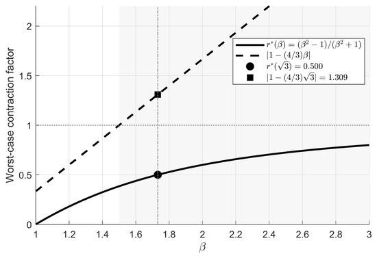
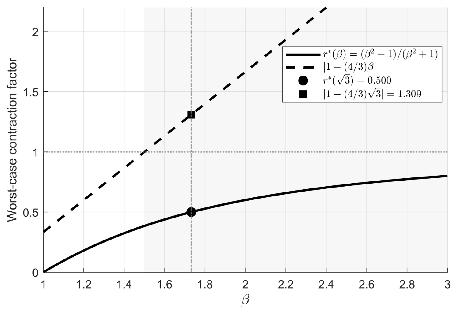
Figure 4 compares the worst-case contraction factors of the proposed reaching gain and the fixed-gain design of [8] as functions of the uncertainty ratio $\beta$. The proposed factor $r^{\star }\left(\beta \right)=({\beta }^2-1)/({\beta }^2+1)$ remains strictly below unity for every finite $\beta$, guaranteeing contraction inside the boundary layer regardless of the uncertainty level. In contrast, the fixed gain $\theta =4/3$ (corresponding to the typical choice $\eta =1$, $\epsilon =0.5$ in [8]) crosses the contraction boundary at $\beta =3/2$ and grows linearly thereafter. At the converter’s operating point $\beta =\sqrt{3}$, the fixed-gain factor reaches $|1-(4/3)\sqrt{3}|=1.309$, meaning the inside-layer iteration amplifies $\sigma$ by 31% per step, whereas the proposed gain yields $r^{\star }=0.500$, halving $\sigma$ at each step.

Figure 4. Worst-case one-step contraction factor versus uncertainty ratio $\beta$: proposed $r^{\star }\left(\beta \right)$ (solid) and fixed $|1-(4/3\left)\beta \right|$ (dashed). The horizontal line at 1 is the contraction boundary; the shaded region indicates $\beta \ge 3/2$, where the fixed gain does not contract. Markers indicate the converter’s operating point at $\beta =\sqrt{3}$.

5.2. System Response Under Constant Irradiance

In this scenario, the system operates under standard test conditions ($G=1000$ W/m², $T=25$ °C) and the MPPT algorithm converges to the MPP. Three battery bank voltages are tested: 24 V, 48 V, and 72 V.

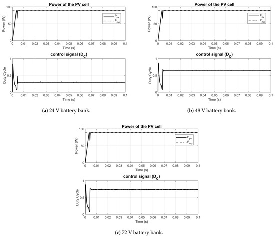
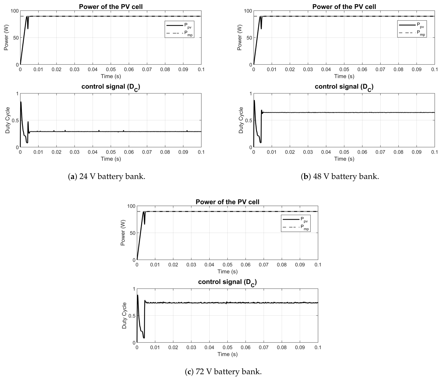
Figure 5 shows the PV panel power extraction and $D_C$ for each battery bank. In all three cases, the MPPT algorithm converges to the rated power $P_{\mathrm{mp}}\approx 90$ W, and $D_C$ settles to the corresponding steady-state operating value $D_C\approx 1-V_{\mathrm{pv}}/V_{\mathrm{bat}}$, where $V_{\mathrm{pv}}$ is the converged MPP voltage. The values differ slightly from the lossless formula due to conduction losses in the power stage.

Figure 5. Steady-state response under constant irradiance ($G=1000$ W/m²). Each subfigure contains two subplots: PV panel power $P_{\mathrm{pv}}$ (top) and $D_C$ (bottom). (a) 24 V battery bank. (b) 48 V battery bank. (c) 72 V battery bank.

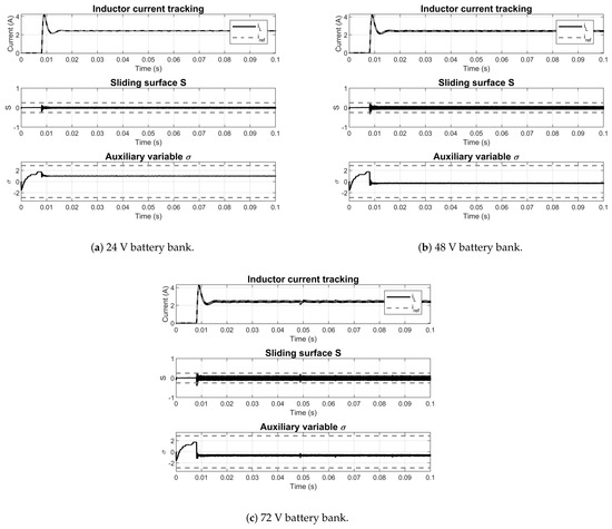
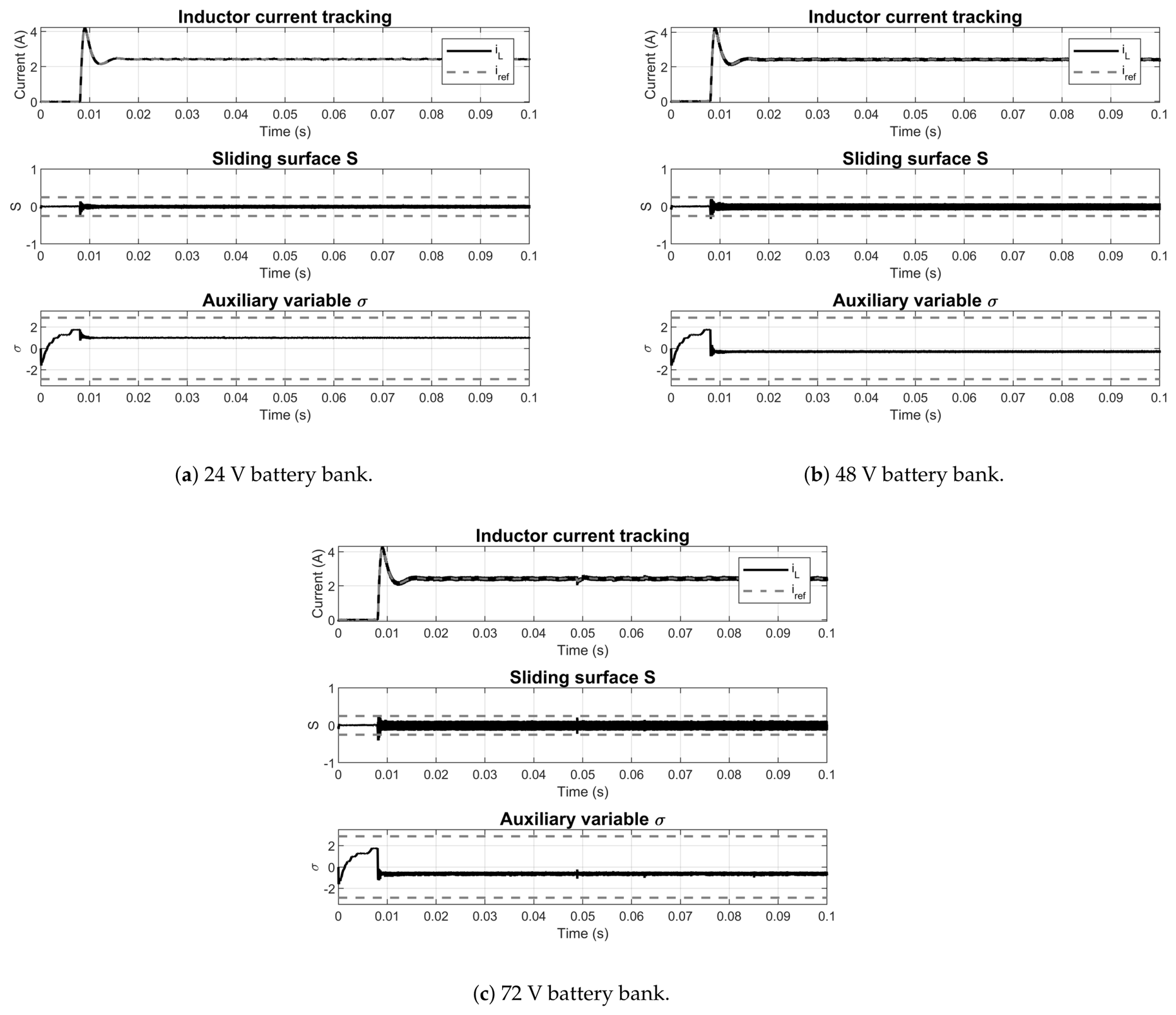
Figure 6 presents the inductor current tracking and the sliding surfaces S and $\sigma$ for each battery bank. The sliding variable $S=i_L-i_{\mathrm{ref}}$ converges to a neighborhood of zero due to the integral action of z, while the ISM variable $\sigma$ remains within the boundary layer $\varphi$. In each subplot, the dashed horizontal lines indicate the theoretical worst-case steady-state bounds: for S, the bound (70) gives ${\left|S\right|}_{\mathrm{ss}}\approx 0.163$ A (where $D_{\max }=1-E_n/V_{C,\max }$ is the highest steady-state duty cycle), accounting for both the one-step residual perturbation that the integrator z has not yet compensated and the inductor current ripple due to pulse-width modulation (PWM) switching; for $\sigma$, the bound ${\left|\sigma \right|}_{\mathrm{ss}}\le T_s\left|P_{\mathrm{ss}}\right|/({\theta }^{\star }\Delta g)\approx 2.87$ A corresponds to the worst-case operating point ($V_{\mathrm{bat}}=24$ V, $\Delta g=0.577$), where the gain mismatch and parasitic losses produce the largest steady-state offset. The offset of $\sigma$ varies with the operating point, scaling linearly with the reference current $i_{\mathrm{ref}}$ and inversely with $\Delta g$, consistent with the parasitic-loss-driven expression (69).

Figure 6. Steady-state current regulation under constant irradiance ($G=1000$ W/m²). Each subfigure contains three subplots: inductor current tracking $i_L$ vs. $i_{\mathrm{ref}}$ (top), sliding variable $S=i_L-i_{\mathrm{ref}}$ (middle), and auxiliary ISM variable $\sigma$ with boundary layer $\pm \varphi$ (bottom). (a) 24 V battery bank. (b) 48 V battery bank. (c) 72 V battery bank.

5.3. Irradiance Step Changes

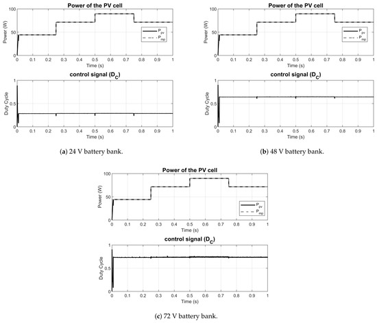
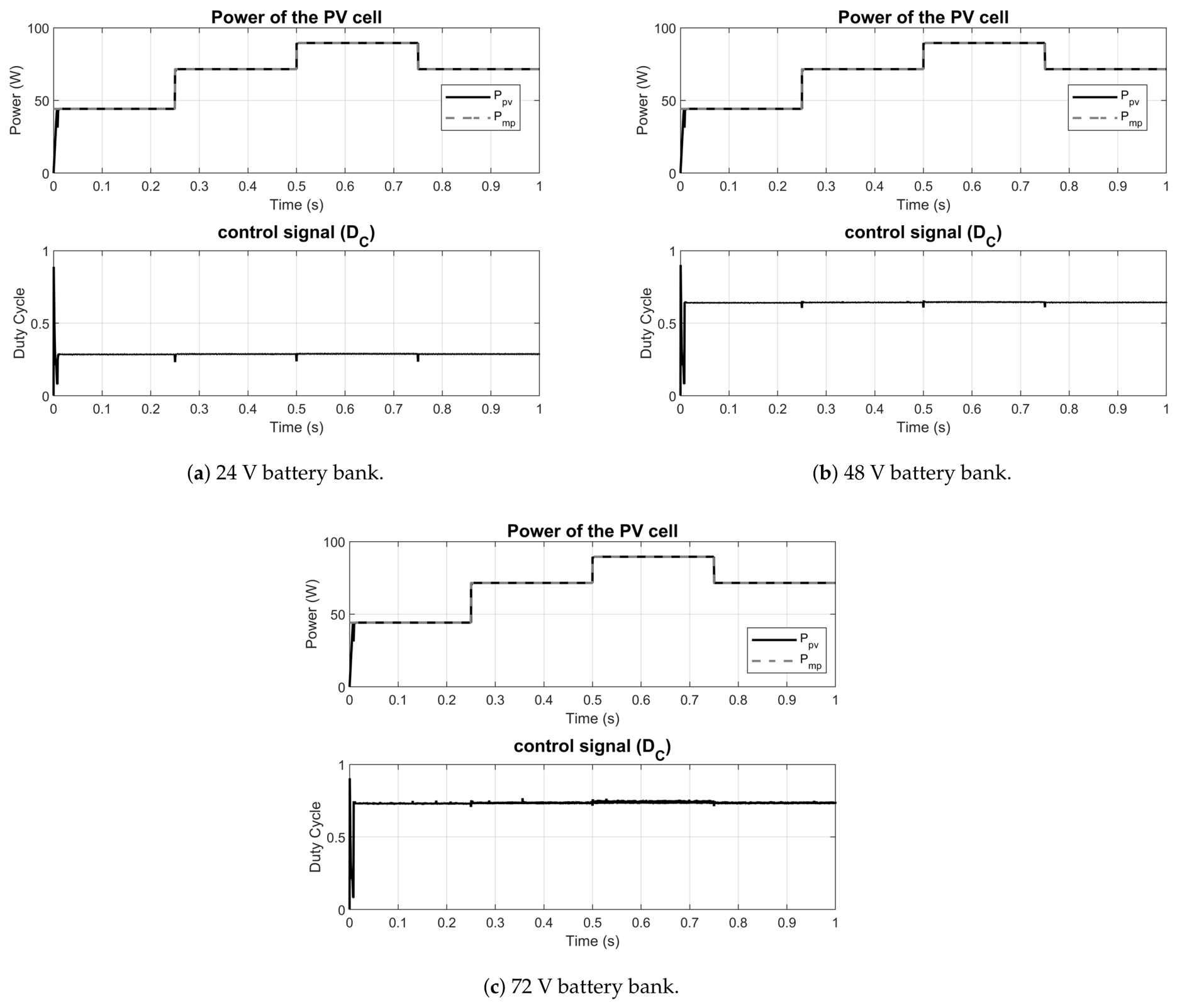
To evaluate the robustness of the controller under external disturbances, irradiance step changes are applied during operation. These steps modify the PV operating point, E, and the $i_{\mathrm{ref}}$ simultaneously, exercising the disturbance rejection capability of the controller. The irradiance profile follows the sequence $G=500\to 800\to 1000\to 800$ W/m², with step transitions at regular intervals of 250 ms. This test exercises both the MPPT tracking capability and the inner-loop disturbance rejection.

Figure 7 shows the PV power and $D_C$ response under irradiance steps for each battery bank. The MPPT algorithm tracks the changing power point, and $D_C$ adjusts accordingly. The controller maintains regulation during the transitions without exhibiting excessive overshoot or instability.

Figure 7. Response under irradiance step changes ($G=500\to 800\to 1000\to 800$ W/m²). Each subfigure contains two subplots: PV panel power $P_{\mathrm{pv}}$ (top) and $D_C$ (bottom). (a) 24 V battery bank. (b) 48 V battery bank. (c) 72 V battery bank.

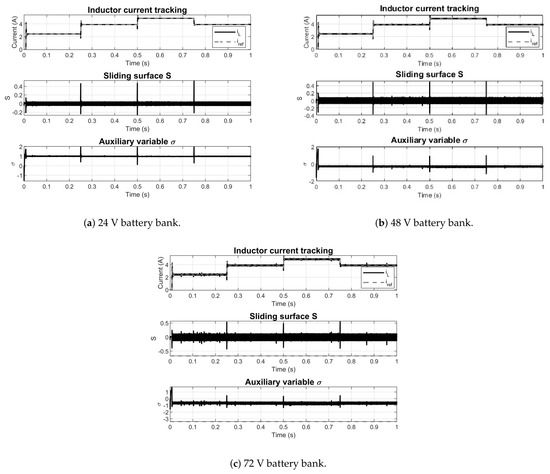
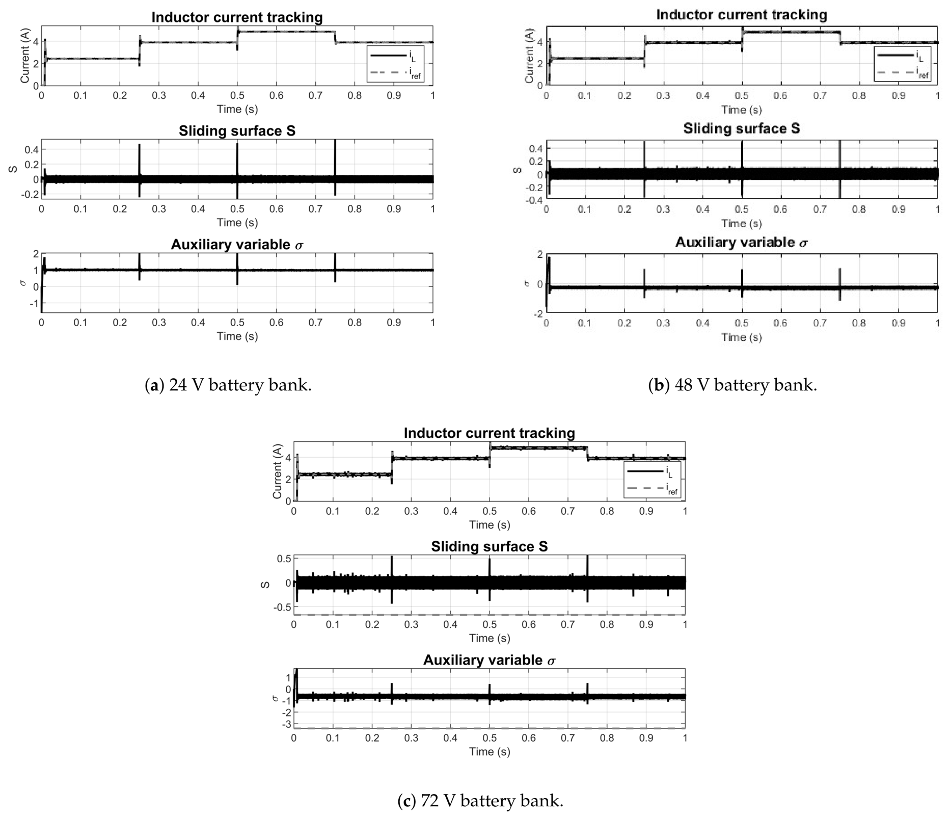
Figure 8 presents the current tracking and sliding surfaces under the same irradiance profile. At each irradiance step, the MPPT updates $i_{\mathrm{ref}}$ and the ISM controller tracks the new reference within a few switching periods. The sliding variable S returns to zero after each transient, and $\sigma$ remains within the boundary layer throughout the test, confirming the robustness guarantees of Theorem 1. The quasi-static offset of $\sigma$ adjusts to the new operating current, consistent with (69).

Figure 8. Current regulation under irradiance step changes ($G=500\to 800\to 1000\to 800$ W/m²). Each subfigure contains three subplots: inductor current tracking $i_L$ vs. $i_{\mathrm{ref}}$ (top), sliding variable $S=i_L-i_{\mathrm{ref}}$ (middle), and auxiliary ISM variable $\sigma$ with boundary layer $\pm \varphi$ (bottom). (a) 24 V battery bank. (b) 48 V battery bank. (c) 72 V battery bank.

5.4. Comparison with a Discrete PI Controller

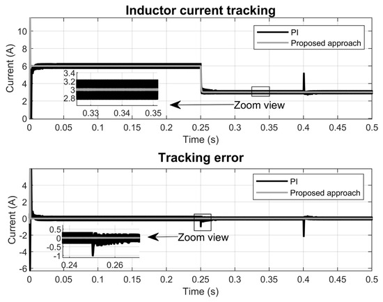
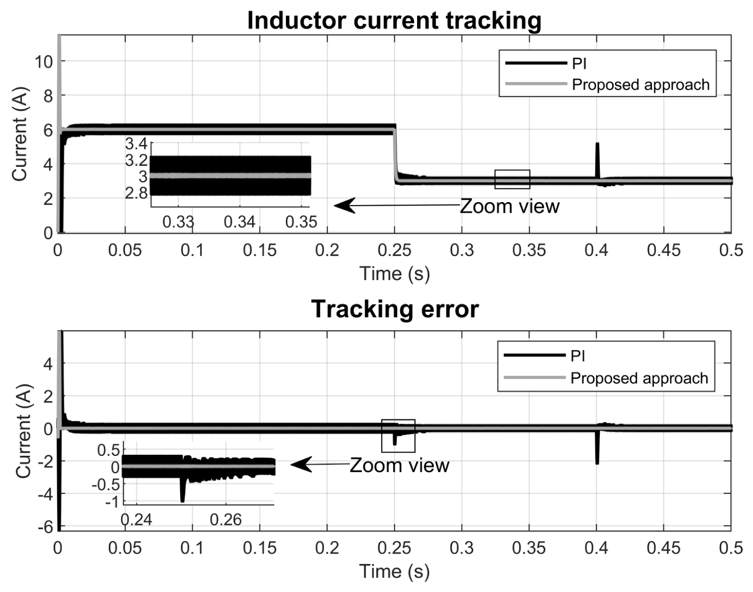
To isolate the effect of the robust compensation from the MPPT dynamics, the proposed ISM controller is compared against a discrete-time PI controller on a simplified test scenario: the PV panel is replaced by a DC voltage source ($E=12$ V) and the battery bank is replaced by a resistive load ($R=10\Omega$), so that the capacitor voltage $V_C$ varies freely with the operating conditions rather than being fixed by the battery. The PI control law is

$$D_C^{\mathrm{PI}}\left[k\right]={\mathrm{sat}}_{[0,1]}\left(D_n-K_{p}e\left[k\right]-K_i{T}_{s}w\left[k\right]\right),$$

(72)

where $e\left[k\right]=i_L\left[k\right]-i_{\mathrm{ref}}\left[k\right]$ is the current error, with integrator state $w\left[k\right]=w[k-1]+e[k-1]$, $w\left[0\right]=0$. The PI gains are selected to match the nominal closed-loop bandwidth of the proposed controller ($k_0=5000$ s⁻¹):

$$K_p={\displaystyle \frac{L_n{k}_0}{V_{C,n}}}\approx 0.0308,K_i={\displaystyle \frac{L_n{k}_0^2}{V_{C,n}}}\approx 153.9.$$

(73)

Both controllers are tested under the same scenario with two sequential disturbances: a reference step from $i_{\mathrm{ref}}=6$ A to 3 A at $t=0.25$ s, and an input voltage step from $E=12$ V to 18 V at $t=0.4$ s. Figure 9 shows the inductor current tracking and the tracking error for both controllers. Three differences are observed: (i) the proposed ISM controller exhibits a smaller inductor current ripple in steady state; (ii) the transient response after the reference step is faster for the ISM controller; and (iii) the ISM controller is less sensitive to the input voltage perturbation, recovering the reference with a smaller deviation and shorter settling time. These improvements are attributed to the robust compensation layer, which rejects the time-varying perturbation through the optimal reaching gain, while the PI relies solely on its finite integral bandwidth.

Figure 9. Comparison between the proposed ISM controller approach and the discrete PI controller with a resistive load ($R=10\Omega$). Top: inductor current $i_L$. Bottom: tracking error $e=i_L-i_{\mathrm{ref}}$. A reference step ($6\to 3$ A) is applied at $t=0.25$ s and an input voltage step ($12\to 18$ V) at $t=0.4$ s.

5.5. Analysis Results

To quantify the performance of the proposed controller, the following metrics are evaluated during the steady-state interval $[n_1,n_2]$ after the MPPT algorithm has converged.

The MPPT tracking efficiency measures the fraction of available PV energy that is effectively extracted:

$${\eta }_{\mathrm{MPPT}}={\displaystyle \frac{{\displaystyle {\displaystyle \sum _{k=n_1}^{n_2}}{P}_{\mathrm{pv}}\left[k\right]}}{{\displaystyle {\displaystyle \sum _{k=n_1}^{n_2}}{P}_{\mathrm{mpp}}\left[k\right]}}}\times 100\%,$$

(74)

where $P_{\mathrm{pv}}\left[k\right]=V_{\mathrm{pv}}\left[k\right]I_{\mathrm{pv}}\left[k\right]$ is the measured PV power and $P_{\mathrm{mpp}}\left[k\right]$ is the theoretical maximum power at the given irradiance and temperature.

The current tracking quality is assessed through the root-mean-square (RMS) value of the normalized current error:

$$e_{\mathrm{RMS}}=\sqrt{{\displaystyle \frac{1}{n_2-n_1+1}}\sum _{k=n_1}^{n_2}{\left({\displaystyle \frac{i_L\left[k\right]-i_{\mathrm{ref}}\left[k\right]}{i_{\mathrm{ref}}\left[k\right]}}\right)}^2}\times 100\%.$$

(75)

Table 5, Table 6 and Table 7 summarize the quantitative results for the three battery banks at irradiance levels of 1000, 800, and 500 W/m², respectively. In all cases, the battery state of charge is set to 50% and all metrics except the startup convergence time are computed after the P&O algorithm has reached the MPP.

Table 5. Performance metrics at $G=1000$ W/m², $T=25$ °C.

Metric	24 V	48 V	72 V
$D_C$	0.289	0.645	0.739
${\eta }_{\mathrm{MPPT}}$ (%)	99.9976	99.9977	99.9977
Startup convergence (ms)	6.312	6.315	6.316
Current error $e_{\mathrm{RMS}}$ (%)	2.0684	4.0113	5.0299

Table 6. Performance metrics at $G=800$ W/m², $T=25$ °C.

Metric	24 V	48 V	72 V
$D_C$	0.288	0.644	0.735
${\eta }_{\mathrm{MPPT}}$ (%)	99.9982	99.9981	99.9982
Startup convergence (ms)	7.121	7.124	7.126
Current error $e_{\mathrm{RMS}}$ (%)	2.0557	4.0318	5.0903

Table 7. Performance metrics at $G=500$ W/m², $T=25$ °C.

Metric	24 V	48 V	72 V
$D_C$	0.285	0.641	0.731
${\eta }_{\mathrm{MPPT}}$ (%)	99.9907	99.9905	99.9909
Startup convergence (ms)	9.435	9.439	9.445
Current error $e_{\mathrm{RMS}}$ (%)	2.0195	4.0401	5.1654

Table 8 compares the proposed ISM controller with the discrete PI controller (72) using the test scenario of Section 5.4 ($i_{\mathrm{ref}}=6$ A, $E=12$ V, $R=10\Omega$). Both controllers use the same nominal bandwidth ($k_0=5000$ s⁻¹).

Table 8. Quantitative comparison between the proposed ISM controller and the discrete PI controller under the test scenario of Section 5.4.

Metric	Proposed ISM Approach	Discrete PI
$e_{\mathrm{RMS}}$ (%)	1.5898	11.371
$\Delta i_L$ (A)	0.07	0.48
Startup time (ms)	2.618	6.521

Remark 14.

The results in Table 5, Table 6 and Table 7 show that the MPPT tracking efficiency remains above a high threshold across all tested conditions. While ${\eta }_{\mathrm{MPPT}}$ remains virtually constant across battery voltages, the normalized $e_{\mathrm{RMS}}$ grows modestly with $D_C$ (from approximately 2% at 24 V to 5% at 72 V), which is attributable to the larger inductor current ripple $\Delta i_L=E{D}_C/\left(L{f}_{\mathrm{sw}}\right)$ at higher duty cycles—an inherent characteristic of the power stage, not a degradation of the controller performance. The MPPT startup convergence time stays within a few milliseconds regardless of the battery voltage.

6. Conclusions

This study investigated the selection of reaching gain in discrete-time sliding mode control under multiplicative gain uncertainty. The main contribution is an optimal reaching-gain design that guarantees contraction within the boundary layer for all finite uncertainty ratios. The principal findings are summarized as follows.

The fixed reaching gain used in Misawa’s saturation-based controller was shown to lose contraction within the boundary layer for gain uncertainty ratios as low as 50%. An optimal reaching gain was derived by reformulating the inside-layer dynamics as a stationary relaxation iteration, yielding a worst-case contraction factor strictly less than 1 for all finite uncertainty ratios. This result establishes a unified framework that connects discrete-time sliding mode control with classical iterative methods from numerical linear algebra and convex optimization for reaching-gain design.

The optimal reaching law was incorporated into a discrete-time ISM structure that is specifically designed to eliminate the reaching phase. This approach advances the main contribution in the boost converter application in two key ways. At voltage extremes, where $\Delta g$ deviates significantly from unity, the direct fixed-gain design diverges within the boundary layer ($J_M>1$), while the proposed controller maintains contraction ($r^{\star }<1$). Near the nominal voltage ($\Delta g\approx 1$), ISM drift cancellation substantially reduces the effective perturbation compared to the uncompensated drift, thereby narrowing the operating $\sigma$-band well below the worst-case design $\varphi$. Furthermore, a past-step disturbance estimator, regulated by a confidence factor to prevent error amplification, was integrated. When the realized gain is close to the nominal value (${\alpha }_{\mathrm{est}}\Delta g\approx 1$), the estimator reduces the quasi-sliding band from $O\left(T_s\right)$ to $O\left(T_s^2\right)$. At the extremes of gain, the improvement diminishes, and the band remains at $O\left(T_s\right)$.

The proposed controller was implemented in a photovoltaic battery charging system using a DC–DC boost converter that serves three battery banks at 24, 48, and 72 V. Simulations with a switching-level model including parasitic elements demonstrated that the inductor current closely tracks the MPPT reference, and the sliding variable converges to a neighborhood of zero. The auxiliary ISM variable remains within the design boundary layer under both constant and time-varying irradiance conditions. Additionally, the steady-state offset of the auxiliary variable was found to scale linearly with the reference current and parasitic resistance, consistent with theoretical predictions. A comparison with a discrete PI controller of matched nominal bandwidth confirmed that the proposed ISM controller achieves smaller inductor current ripple, faster transient response, and reduced sensitivity to input voltage perturbations.

Future research directions include experimental validation of the proposed controller on embedded platforms, extension to multi-input topologies such as interleaved boost converters, and investigation of semi-iterative Chebyshev acceleration strategies for fixed but unknown gain uncertainty.

References

- Utkin, V.I. Variable structure systems with sliding modes. IEEE Trans. Autom. Control 1977, 22, 212–222. [Google Scholar] [CrossRef] [Scilit]
- Edwards, C.; Spurgeon, S.K. Sliding Mode Control: Theory and Applications; CRC Press: Boca Raton, FL, USA, 1998. [Google Scholar]
- Utkin, V.; Guldner, J.; Shi, J. Sliding Mode Control in Electro-Mechanical Systems, 2nd ed.; CRC Press: Boca Raton, FL, USA, 2017. [Google Scholar]
- Milosavljević, Č. General Conditions for the Existence of a Quasi-Sliding Mode on the Switching Hyperplane in Discrete Variable Structure Systems. Autom. Remote Control 1985, 46, 307–314. [Google Scholar]
- Gao, W.; Wang, Y.; Homaifa, A. Discrete-Time Variable Structure Control Systems. IEEE Trans. Ind. Electron. 1995, 42, 117–122. [Google Scholar] [CrossRef] [Scilit]
- Sarpturk, S.Z.; Istefanopulos, Y.; Kaynak, O. On the Stability of Discrete-Time Sliding Mode Control Systems. IEEE Trans. Autom. Control 1987, 32, 930–932. [Google Scholar] [CrossRef] [Scilit]
- Furuta, K. Sliding Mode Control of a Discrete System. Syst. Control Lett. 1990, 14, 145–152. [Google Scholar] [CrossRef] [Scilit]
- Misawa, E.A. Discrete-Time Sliding Mode Control for Nonlinear Systems with Unmatched Uncertainties and Uncertain Control Vector. Asme J. Dyn. Syst. Meas. Control 1997, 119, 503–512. [Google Scholar] [CrossRef] [Scilit]
- Bartoszewicz, A. Discrete-Time Quasi-Sliding-Mode Control Strategies. IEEE Trans. Ind. Electron. 1998, 45, 633–637. [Google Scholar] [CrossRef] [Scilit]
- Bandyopadhyay, B.; Janardhanan, S. Discrete-Time Sliding Mode Control: A Multirate Output Feedback Approach; Springer: Berlin/Heidelberg, Germany, 2006; Volume 323. [Google Scholar]
- Acary, V.; Brogliato, B. Implicit Euler Numerical Scheme and Chattering-Free Implementation of Sliding Mode Systems. Syst. Control Lett. 2010, 59, 284–293. [Google Scholar] [CrossRef] [Scilit]
- Brogliato, B.; Polyakov, A.; Efimov, D. The Implicit Discretization of the Supertwisting Sliding-Mode Control Algorithm. IEEE Trans. Autom. Control 2019, 65, 3707–3713. [Google Scholar] [CrossRef] [Scilit]
- Koch, S.; Reichhartinger, M. Discrete-Time Equivalents of the Super-Twisting Algorithm. Automatica 2019, 107, 190–199. [Google Scholar] [CrossRef] [Scilit]
- Fridman, L.; Moreno, J.; Iriarte, R. Sliding Modes After the First Decade of the 21st Century; Springer: Berlin/Heidelberg, Germany, 2012. [Google Scholar]
- Brogliato, B.; Polyakov, A. Digital Implementation of Sliding-Mode Control via the Implicit Method: A Tutorial. Int. J. Robust. Nonlinear Control 2021, 31, 3528–3586. [Google Scholar] [CrossRef] [Scilit]
- Latosiński, P.; Adamiak, K. Discrete-Time Sliding Mode Control Strategies—State of the Art. Energies 2024, 17, 4564. [Google Scholar] [CrossRef] [Scilit]
- Utkin, V.; Shi, J. Integral sliding mode in systems operating under uncertainty conditions. In Proceedings of the 35th IEEE Conference on Decision and Control, Kobe, Japan, 11–13 December 1996; pp. 4591–4596. [Google Scholar]
- Cao, W.J.; Xu, J.X. Nonlinear integral-type sliding surface for both matched and unmatched uncertain systems. IEEE Trans. Autom. Control 2004, 49, 1355–1360. [Google Scholar] [CrossRef] [Scilit]
- Rubagotti, M.; Estrada, A.; Castanos, F.; Ferrara, A.; Fridman, L. Integral sliding mode control for nonlinear systems with matched and unmatched perturbations. IEEE Trans. Autom. Control 2011, 56, 2699–2704. [Google Scholar] [CrossRef] [Scilit]
- Su, W.C.; Drakunov, S.V.; Özgüner, U. An O(T2) Boundary Layer in Sliding Mode for Sampled-Data Systems. IEEE Trans. Autom. Control 2000, 45, 482–485. [Google Scholar] [CrossRef] [Scilit]
- Drakunov, S.V.; Utkin, V.I. Sliding Mode Control in Dynamic Systems. In Proceedings of the 32nd IEEE Conference on Decision and Control, San Antonio, TX, USA, 15–17 December 1993; pp. 2446–2451. [Google Scholar]
- Bianconi, E.; Calvente, J.; Giral, R.; Mamarelis, E.; Petrone, G.; Ramos, P.C.; Spagnuolo, G.; Vitelli, M. Perturb and observe MPPT algorithm with a current controller based on the sliding mode. Int. J. Electr. Power Energy Syst. 2013, 44, 346–356. [Google Scholar] [CrossRef] [Scilit]
- Montoya, D.G.; Ramos-Paja, C.A.; Giral, R. Improved Design of Sliding-Mode Controllers Based on the Requirements of MPPT Techniques. IEEE Trans. Power Electron. 2016, 31, 235–247. [Google Scholar] [CrossRef] [Scilit]
- Chinnappan, R.; Logamani, P.; Ramasubbu, R. Fixed frequency integral sliding-mode current-controlled MPPT boost converter for two-stage PV generation system. IET Circuits Devices Syst. 2019, 13, 793–805. [Google Scholar] [CrossRef] [Scilit]
- Fekik, A.; Hamida, M.L.; Azar, A.T.; Ghanes, M.; Hakim, A.; Denoun, H.; Hameed, I.A. Robust power control for PV and battery systems: Integrating sliding mode MPPT with dual buck converters. Front. Energy Res. 2024, 12, 1380387. [Google Scholar] [CrossRef] [Scilit]
- Djanssou, D.M.; Dadjé, A.; Tom, A.; Djongyang, N. Improvement of the dynamic response of robust sliding mode MPPT controller-based PSO algorithm for PV systems under fast-changing atmospheric conditions. Int. J. Photoenergy 2021, 2021, 6671133. [Google Scholar] [CrossRef] [Scilit]
- Levant, A. Sliding order and sliding accuracy in sliding mode control. Int. J. Control 1993, 58, 1247–1263. [Google Scholar] [CrossRef] [Scilit]
- Dunna, V.K.; Chandra, K.P.B.; Rout, P.K.; Sahu, B.K.; Manoharan, P.; Alsoud, A.R.; Derebew, B. Super-twisting MPPT control for grid-connected PV/battery system using higher order sliding mode observer. Sci. Rep. 2024, 14, 16597. [Google Scholar] [CrossRef] [Scilit] [PubMed]
- Cucuzzella, M.; Incremona, G.P.; Ferrara, A. Design of Robust Higher Order Sliding Mode Control for Microgrids. IEEE J. Emerg. Sel. Top. Circuits Syst. 2015, 5, 393–401. [Google Scholar] [CrossRef] [Scilit]
- Inomoto, R.S.; de Almeida Monteiro, J.R.B.; Sguarezi Filho, A.J. Boost Converter Control of PV System Using Sliding Mode Control with Integrative Sliding Surface. IEEE J. Emerg. Sel. Top. Power Electron. 2022, 10, 5522–5530. [Google Scholar] [CrossRef] [Scilit]
- Gursoy, M.; Zhuo, G.; Lozowski, A.G.; Wang, X. Photovoltaic Energy Conversion Systems with Sliding Mode Control. Energies 2021, 14, 6071. [Google Scholar] [CrossRef] [Scilit]
- Sabzehgar, R.; Ghali, R.; Fajri, P. A Novel Combined Control Strategy for a Two-Stage Parallel Full-Wave ZCS Quasi Resonant Boost Converter for PV-Based Battery Charging Systems with Maximum Power Point Tracking. Electricity 2022, 3, 145–161. [Google Scholar] [CrossRef] [Scilit]
- González-Castro, J.A.; Rubio-Astorga, G.J.; Alarcón-Carbajal, M.A.; Sánchez-Torres, J.D.; Medina-Melendrez, M.; Cabanillas-Noris, J.C.; Castro-Palazuelos, D.E. Low-Cost Platform Implementation of Discrete Controllers for DC-DC Boost Converter. Energies 2024, 17, 4097. [Google Scholar] [CrossRef] [Scilit]
- González-Castro, J.A.; Rubio-Astorga, G.J.; Castro-Rubio, J.R.; Alarcón-Carbajal, M.A.; Picos-Ponce, J.C.; Sánchez-Torres, J.D.; Castro-Palazuelos, D.E. Integrated Sliding Mode Control and Adaptive-Step P&O MPPT Strategy for DC–DC Boost–Buck Converter in Photovoltaic Systems. Energies 2026, 19, 1123. [Google Scholar] [CrossRef] [Scilit]
- Varga, R.S. Matrix Iterative Analysis; Prentice-Hall: Englewood Cliffs, NJ, USA, 1962. [Google Scholar]
- Nesterov, Y. Lectures on Convex Optimization, 2nd ed.; Springer: Berlin/Heidelberg, Germany, 2018. [Google Scholar]
- Erickson, R.W.; Maksimović, D. Fundamentals of Power Electronics, 3rd ed.; Springer: Berlin/Heidelberg, Germany, 2020. [Google Scholar]
- Mohan, N.; Undeland, T.M.; Robbins, W.P. Power Electronics: Converters, Applications, and Design, 3rd ed.; John Wiley & Sons: Hoboken, NJ, USA, 2003. [Google Scholar]
- Bacha, S.; Munteanu, I.; Bratcu, A.I. Power Electronic Converters Modeling and Control; Springer: Berlin/Heidelberg, Germany, 2014. [Google Scholar]
- Villalva, M.G.; Gazoli, J.R.; Filho, E.R. Comprehensive Approach to Modeling and Simulation of Photovoltaic Arrays. IEEE Trans. Power Electron. 2009, 24, 1198–1208. [Google Scholar] [CrossRef] [Scilit]
- Richardson, L.F. The Approximate Arithmetical Solution by Finite Differences of Physical Problems Involving Differential Equations, with an Application to the Stresses in a Masonry Dam. Philos. Trans. R. Soc. London. Ser. A 1911, 210, 307–357. [Google Scholar] [CrossRef] [Scilit]
- Femia, N.; Petrone, G.; Spagnuolo, G.; Vitelli, M. Optimization of Perturb and Observe Maximum Power Point Tracking Method. IEEE Trans. Power Electron. 2005, 20, 963–973. [Google Scholar] [CrossRef] [Scilit]
Disclaimer/Publisher’s Note: The statements, opinions and data contained in all publications are solely those of the individual author(s) and contributor(s) and not of MDPI and/or the editor(s). MDPI and/or the editor(s) disclaim responsibility for any injury to people or property resulting from any ideas, methods, instructions or products referred to in the content. |
© 2026 by the authors. Licensee MDPI, Basel, Switzerland. This article is an open access article distributed under the terms and conditions of the Creative Commons Attribution (CC BY) license.