


Abstract
This paper presents an experimental investigation of dynamic line rating (DLR) applied to aluminium conductor steel-reinforced (ACSR) overhead line conductors, with a specific focus on wind speed conditions up to 5 m/s. An experimental system was designed and implemented to provide controlled and repeatable cross-flow air conditions along a tested ACSR conductor, enabling direct measurement of wind speed in the immediate vicinity of the conductor surface. Conductor temperature, electrical current, voltage drop per unit length, the phase angle between them, and relevant meteorological parameters were continuously measured under controlled experimental conditions. Based on the measured data, the conductor heat balance was evaluated and the allowable current-carrying capacity was determined. The experimentally obtained conductor temperatures and ampacity values were compared with results calculated using thermal models and correlations recommended by IEEE, CIGRÉ, and IEC standards. The comparison demonstrates that, under low and moderate wind speed conditions, differences between standard-based predictions and experimental results can be significant, leading to deviations in the estimation of allowable current-carrying capacity. The results confirm the high sensitivity of DLR calculations to wind-related assumptions and provide an experimentally validated basis for assessing the applicability and limitations of existing standard thermal models for ACSR conductors under realistic operating conditions.
1. Introduction
The continuous growth of global electricity consumption, accelerated by the intensive integration of renewable energy sources (RESs) and the increasing electrification of various sectors, has led to a substantial increase in the loading of existing transmission networks [1]. At the same time, the construction of new overhead transmission lines (OHTLs) represents a technically complex, capital-intensive process that is often constrained by spatial, regulatory, and environmental factors [2]. Under such conditions, enhancing the utilization of existing transmission infrastructure has become one of the key strategic objectives of modern power systems.
One of the most effective approaches to achieving this objective is the application of Dynamic Line Rating (DLR) for overhead transmission lines. In contrast to traditional Static Line Rating (SLR) methods, which are based on conservative assumptions and worst-case meteorological conditions, DLR enables the determination of the allowable current based on actual or forecasted environmental conditions [3,4,5]. Previous studies [5,6,7,8] have demonstrated that the application of DLR can increase the transmission capacity of existing lines by 10–30% without any infrastructure interventions. Similar conclusions regarding the benefits of DLR and the comparison between theoretical thermal models and experimental measurements were also reported in recent studies focusing on advanced overhead conductors and real operating conditions [9].
DLR calculations are fundamentally based on the conductor heat balance equation, in which the conductor temperature is determined by the equilibrium between internal heat generation and heat dissipation mechanisms to the surrounding environment [3,4,10]. Although Joule heating losses dominate under most operating conditions, meteorological parameters, particularly wind speed and wind direction, play a decisive role in convective cooling and, consequently, in the assessment of allowable current-carrying capacity (also known as “ampacity”) [2,5,11]. Due to its pronounced spatial and temporal variability, wind has been identified as the most critical and, at the same time, the most uncertain input parameter in DLR calculations [5,6,11]. Meteorological parameters such as wind speed, ambient temperature, and solar radiation represent the most influential factors affecting conductor thermal balance and DLR calculations [12,13].
A particularly sensitive operating regime corresponds to low wind speeds, typically below 5 m/s. In this range, convective heat transfer exhibits strongly nonlinear behavior, such that even minor deviations in assumptions regarding wind speed or flow direction can result in significant differences in the calculated conductor temperature and ampacity. Experimental studies indicate that, under low-wind-speed conditions, discrepancies between different standardized thermal models are most pronounced, and substantial deviations between model predictions and experimentally measured values may occur [5,6]. A comprehensive overview of DLR technology, including monitoring systems and thermal rating models, has been presented in recent review studies [12].
The most commonly used models for calculating the ampacity of OHTLs are defined in the IEEE [3], CIGRÉ [4], and IEC [10] standards. Although these standards are based on the same physical foundation, namely the heat balance equation, they employ different empirical correlations for modeling natural and forced convection, as well as different assumptions regarding conductor surface temperature and airflow regimes. Comparative analyses have shown that these differences can lead to significant deviations in the estimated ampacity [5,6,7,8].
Despite the fact that a number of studies addressing the modeling and application of DLR have been published in recent years [14,15,16,17,18], systematic experimental verification of standard-recommended thermal models under controlled conditions and at low wind speeds remains limited [5,6,7,9,19]. Most available studies rely on field measurements, which are inherently affected by substantial uncertainties related to the spatial homogeneity of wind, local turbulence effects, and the accuracy of meteorological data [6,7]. Consequently, direct comparison of standardized thermal models with experimentally measured conductor temperatures and current-carrying capacities under strictly controlled conditions remains an open and insufficiently investigated research problem.
In addition to uncertainties associated with convective heat transfer, the emissivity of OHTL conductors represents another critical parameter affecting the accuracy of thermal rating calculations. In existing standards and much of the published literature, the emissivity of ACSR conductors is commonly assumed to be an approximately known and constant value, typically selected based on generalized surface condition categories. However, growing experimental evidence indicates that emissivity is not a fixed material constant, but a surface-dependent parameter that varies significantly with conductor aging, oxidation, contamination, and environmental exposure [20]. Such variations directly influence radiative heat dissipation and can lead to non-negligible deviations in calculated conductor temperature and ampacity, particularly under low wind speed conditions where radiative and convective heat losses become comparable. Consequently, the use of fixed tabulated emissivity values may introduce additional uncertainty into DLR assessments, highlighting the need for experimental identification of emissivity under controlled and well-defined conditions.
In addition to uncertainties related to convective heat transfer and surface emissivity, the accurate determination of the AC electrical resistance of ACSR conductors represents another critical factor influencing the reliability of DLR-based thermal models. In standard calculation procedures, the AC resistance is commonly treated as a function of conductor temperature only, with current-dependent effects implicitly neglected or incorporated through simplified correction factors. However, for ACSR conductors, numerous experimental and analytical studies have demonstrated that the AC resistance may exhibit a pronounced dependence on current magnitude due to magnetic losses in the steel core, non-uniform current distribution in helically stranded aluminum layers, and the so-called transformer effect [3,4,21,22,23,24]. These phenomena are particularly significant for conductors with an odd number of aluminum layers, where the axial magnetic flux is closed through the ferromagnetic core, leading to resistance increases that may reach 25% relative to low-current values. Neglecting the current dependence of AC resistance directly affects the estimation of Joule losses and conductor temperature, thereby introducing an additional source of error into DLR calculations, especially under operating conditions where thermal margins are limited. Experimental studies on single-layer ACSR conductors have also been conducted to investigate their electromagnetic and thermal behaviour under different operating conditions, including the influence of eddy currents and hysteresis losses in the steel core [25]. Although single-layer ACSR conductors are less frequently used in modern transmission-level DLR applications due to their relatively smaller cross-section and current-carrying capability, their simpler structure makes them a useful reference configuration for analysing the influence of conductor topology on AC resistance and thermal behaviour.
It should be emphasized that reliable experimental verification of DLR thermal models requires the simultaneous and accurate determination of several mutually coupled parameters. In particular, conductor emissivity, wind speed, and AC electrical resistance directly govern radiative heat losses, convective cooling intensity, and Joule heating, respectively. In many previously published studies, these quantities were either assumed, indirectly estimated, or treated using simplified or tabulated values, which limits the reliability of the resulting thermal assessments [3,4,7,10,16,17]. In contrast, the present work performs a systematic comparison of standard-recommended thermal models using experimentally identified conductor emissivity, precisely measured and spatially homogeneous wind speed, and AC resistance determined directly from electrical measurements, including its dependence on operating current. By jointly accounting for these three critical parameters under controlled laboratory conditions, the proposed approach significantly reduces modeling uncertainty and enables a more physically consistent and accurate evaluation of DLR thermal models, particularly in low wind speed regimes.
To the best of the authors’ knowledge, one of the most significant experimental contributions to the analysis of heat losses under low wind speed conditions was provided by J. R. Riba, who conducted a comprehensive experimental investigation of overhead conductor behavior in weak airflow regimes using controlled laboratory conditions, with particular emphasis on the influence of low wind speeds on convective cooling [7]. However, this investigation was limited to a single representative ACSR conductor (i.e., 550-AL1/71-ST1A) and a relatively narrow range of wind speeds (0–3 m/s), without a systematic assessment of the behavior of different ACSR conductors with varying structural configurations.
Furthermore, the available literature lacks experimental studies that consistently and comparatively examine multiple ACSR conductors over a broader range of low wind speeds, including very low wind speed regimes, while simultaneously ensuring stable and spatially homogeneous cross-flow conditions along the entire active conductor section. In the present work, these limitations are addressed through the application of a specially designed diffuser capable of generating controlled, stable, and spatially homogeneous cross-flow airflow, which has not been systematically reported in previous experimental DLR investigations.
Based on the above considerations, the objective of this paper is the experimental verification of thermal models recommended by the IEEE, CIGRÉ, and IEC standards for the calculation of DLR of ACSR overhead line conductors, with a particular focus on low and moderate wind speed conditions. An experimental system was developed to provide controlled and repeatable cross-flow airflow, as well as direct measurement of conductor and ambient temperatures, local wind speed, and relevant electrical parameters. The experimentally obtained results are directly compared with calculations based on IEEE, CIGRÉ, and IEC models, enabling a critical assessment of their accuracy, applicability, and limitations under realistic operating conditions.
2. Materials and Methods
2.1. Thermal Balance Equations for Line Rating Calculations
The calculation of the ampacity of OHTL conductors is based on the energy (thermal) balance equation, in which equilibrium is established between heat generation mechanisms and heat dissipation mechanisms. Differences in the calculated ampacity values obtained using various standards arise both from differences in the formulation of the thermal balance equation itself and from variations in the empirical correlations used to determine heat transfer coefficients for natural convection, forced convection, and radiation.
The procedures recommended by the IEEE, CIGRÉ, and IEC standards are based on the following steady-state thermal balance equations:
- CIGRÉ method [4]:
- IEEE [3] and IEC [10] methods:where PJ is the Joule heating, PS is the solar heating, PM is the magnetic heating, Pi is the corona heating, Pc is the convective cooling, Pr is the radiative cooling and Pw is the evaporative cooling; all quantities are given per unit conductor length in W/m.
In the CIGRE procedure [4], it is commonly assumed that the thermal contributions from the corona heating (Pi) and evaporative cooling (Pw) are disregarded. Consequently, the line ratings obtained through these procedures will inherently differ because the IEEE [3] and IEC [10] assume that magnetic heating (PM) is neglected.
In the present study, the experimental investigation was carried out under controlled indoor laboratory conditions. Since the tests were performed without exposure to solar radiation, the solar heating term does not contribute to the thermal balance and was therefore set to zero, PS = 0. This assumption is consistent with laboratory-based DLR studies reported in the literature and enables an isolated analysis of convective and radiative heat transfer mechanisms [5].
In practice, operating and environmental conditions change, whereas ampacity calculations are conducted at specific intervals. In such scenarios, a non-steady-state heat balance equation can be employed, as follows [3]:
where m is the mass per unit length of the conductor in kg/m, c is the specific heat capacity of the conductor in J/(kg·K), Tc is the conductor temperature in K, and t is the time in s.
The IEEE, CIGRE, and IEC methods employ nearly identical formulas for determining the Joule heating, solar heating, and radiative cooling of OHTL conductors. These terms are based on the same physical principles and differ only marginally in the definition of auxiliary parameters or reference conditions. Consequently, discrepancies in calculated ampacity among the standards originate predominantly from the treatment of convective cooling, while the remaining heat balance components can be considered equivalent.
2.1.1. Joule Heating
Joule heating represents the internally generated thermal power resulting from the flow of electrical current through the conductor and is expressed as:
where I is the RMS conductor current in A, and Rac(Tc) is the AC electrical resistance of the conductor at temperature Tc in Ω/m.
This formulation is identical in the IEEE, CIGRÉ, and IEC standards, as all three approaches model Joule losses as proportional to the square of the current and the temperature-dependent AC resistance of the conductor. Consequently, differences in the calculated Joule heating do not originate from the mathematical form of the equation itself, but rather from the method used to determine the AC resistance.
In standard-based implementations, particularly in IEEE Std 738 [3], the AC electrical resistance of the conductor is most commonly treated as a function of temperature only. The resistance at an arbitrary average conductor temperature Tavg is typically obtained either directly from tabulated values provided by the standard or by applying linear interpolation between two reference temperatures Tlow and Thigh, according to:
Alternatively, the temperature dependence of AC resistance may be expressed using a linear temperature coefficient:
where Rac,0 is the AC electrical resistance of the conductor at the reference temperature T0 (typically 20 °C), and αac is the temperature coefficient of AC resistance in 1/°C.
Both formulations implicitly assume that the AC resistance depends solely on temperature and is independent of the operating current. While this assumption is generally acceptable for homogeneous stranded conductors, it may lead to significant inaccuracies when applied to ACSR conductors, where magnetic effects in the steel core and non-uniform current distribution introduce a pronounced current dependence of Rac [26,27].
Although, for any fixed current level, the AC resistance of an ACSR conductor can be accurately described by a linear function of temperature, this relationship is not universal across different current levels. With increasing current, the reference AC resistance increases due to magnetic losses in the steel core and non-uniform current distribution, while the temperature coefficient remains approximately constant, being governed primarily by the resistivity of aluminum. Accordingly, the AC resistance can be expressed as follows [26]:
where Rac,0(I) is the current-dependent reference AC resistance at the reference temperature T0, while the temperature coefficient of AC resistance remains nearly invariant with respect to current. As a result, the Rac(T) characteristics corresponding to different current levels are shifted almost in parallel, confirming that a single global temperature-dependent resistance model is not applicable to ACSR conductors. Since the AC resistance of ACSR conductors may exhibit a pronounced dependence on current magnitude, the resistance used in the present study was determined experimentally, as described in Section 2.2.
2.1.2. Solar Heat Gain
Under outdoor operating conditions, the solar heat gain of an overhead conductor is commonly expressed as:
where αs is the solar absorptivity, D is the outer conductor diameter in m, and IT is the global solar radiation intensity in W/m2. However, since all experiments in this study were conducted indoors under controlled laboratory conditions without solar exposure, the solar heat gain term was neglected (PS = 0). This assumption is consistent with previous experimental DLR studies performed under laboratory conditions [5].
2.1.3. Radiative Cooling
Radiative cooling represents the heat loss from the conductor surface due to thermal radiation emitted toward the surrounding environment. In all three standards, IEEE 738 [3], CIGRÉ 601 [4], and IEC 61597 [10], radiative heat transfer is described using the Stefan–Boltzmann law and is formulated as a function of conductor emissivity, conductor diameter, and the temperature difference between the conductor surface and ambient air.
The radiative heat loss per unit length of the conductor is given by:
where ε is the emissivity of the conductor surface, σSB is the Stefan–Boltzmann constant, and Ta is the ambient air temperature in K. The same formulation is employed in all three standards, with differences limited to unit conventions and numerical constants, while the underlying physical model remains identical.
2.1.4. Convective Cooling
Convective cooling represents the dominant heat dissipation mechanism for overhead transmission line conductors under most operating conditions, particularly at low and moderate wind speeds. The magnitude of convective heat loss depends strongly on wind speed, airflow regime, conductor geometry, and the temperature difference between the conductor surface and the surrounding air. Consequently, the treatment of convective cooling constitutes the primary source of discrepancy among the IEEE, CIGRÉ, and IEC thermal rating standards. In all three standards, the convective heat loss per unit length of the conductor can be expressed in the general form:
where hc is the convective heat transfer coefficient in W/(m2∙K).
Under forced convection conditions, the heat transfer coefficient is obtained via the Nusselt number (Nu) according to
where kf is the thermal conductivity of air evaluated at the film temperature in W/(m∙K).
The Nusselt number is defined through empirical correlations that depend on the assumed convection regime and relevant dimensionless numbers. The fundamental differences among the standards arise from the selection of these correlations and the treatment of different convection regimes.
IEEE Std 738
In this standard, convective cooling is treated by distinguishing between forced and natural convection regimes, with heat transfer evaluated using empirical correlations originally proposed by McAdams for cross-flow over circular cylinders. Forced convection is expressed primarily as a function of the Reynolds number, while natural convection is considered under still-air or near-zero wind conditions. At low wind speeds, IEEE recommends calculating both forced and natural convection components and adopting the larger of the two values, resulting in a conservative estimate of convective cooling.
For forced convection, the convective heat loss per unit length is given by [3]
or alternatively
where Kangle is the wind-angle correction factor (equal to 1 for perpendicular flow). IEEE recommends calculating both expressions and selecting the larger value of Pc,f.
In the IEEE formulation, the convective heat transfer coefficient hc is implicitly defined through the McAdams correlations, such that Equations (12) and (13) represent specific realizations of the general convective heat loss expression given in Equation (10). The Reynolds number (Re) is defined as a function of the wind speed in the following manner:
where ρf is the air density in kg/m3, v is the wind speed in m/s, and μf is the dynamic viscosity of the air in kg/(m∙s).
Under zero or near-zero wind speed conditions, natural convection is expressed as
where all air properties are evaluated at the film temperature.
CIGRÉ TB 601
In the CIGRÉ methodology, convective cooling is treated within a unified framework that explicitly accounts for natural, forced, and mixed convection regimes. Unlike the IEEE approach, which evaluates natural and forced convection separately and adopts the larger value, the CIGRÉ method determines the dominant heat transfer mechanism based on dimensionless similarity criteria and applies the corresponding empirical correlation.
Under forced convection conditions the Nusselt number is expressed as [4]
where B and n are empirical coefficients recommended for forced convection under steady cross-flow conditions. The coefficients depend on the Reynolds number range and the effective surface roughness of the conductor, with distinct values specified for smooth and stranded conductors [4].
In still-air or very low wind speed conditions, the convective cooling is governed by natural convection. The corresponding Nusselt number is expressed as
where A and m are empirical coefficients determined as functions of the product Gr⋅Pr, with Gr denoting the Grashof number and Pr the Prandtl number. The applicable values of A and m are selected according to the corresponding Gr⋅Pr range, as specified in [4].
IEC 61597
According to IEC 61597, the convective cooling of overhead conductors is evaluated exclusively under forced convection conditions. Natural convection effects are not explicitly modelled; instead, the heat transfer process is described assuming steady cross-flow of air perpendicular to the conductor axis.
The Nusselt number is calculated using the empirical correlation [10]
which is valid for forced convection over a cylindrical conductor under cross-flow conditions. The convective heat loss per unit length is subsequently obtained using Equations (10) and (11), with the Nusselt number defined by Equation (18).
The Reynolds number is defined as
Unlike IEEE Std 738 and CIGRÉ TB 601, the IEC 61597 methodology considers only forced convection heat transfer and does not provide a separate formulation for natural convection. Consequently, it does not distinguish between natural, forced, or mixed convection regimes. As a result, the IEC approach offers a simplified and computationally efficient formulation, but may exhibit reduced accuracy under low wind speed conditions where buoyancy-driven heat transfer becomes significant.
In the present experimental investigation, the airflow was maintained perpendicular to the conductor axis (β = 90°), which is fully consistent with the assumptions underlying the IEC forced-convection model.
2.2. Determination of AC Resistance
The AC electrical resistance of the investigated ACSR conductors was determined experimentally under controlled laboratory conditions. Unlike standard-based approaches, where the AC resistance is commonly assumed to be a known function of conductor temperature only, the present study relies on direct electrical measurements in order to capture the combined influence of temperature and current magnitude on the resistance behavior. All measurements were performed under sinusoidal excitation at the power frequency of 50 Hz. During each test, the conductor was energized with a controlled alternating current, while the RMS current I, the voltage drop per unit length ΔU, and the phase angle φ between them were continuously measured.
The measurements were conducted under quasi-steady-state thermal conditions, for which the temporal variation in the conductor temperature was negligible during each measurement interval. Following the recommendations of CIGRÉ TB 345, the AC resistance per unit length was calculated from the measured quantities as:
This method enables accurate extraction of the resistive component of the impedance and reliable determination of AC resistance, even in the presence of inductive and magnetic phenomena characteristic of ACSR conductors. To allow comparison of resistance values obtained under different thermal conditions, the measured AC resistance was referred to a chosen reference temperature using the linear temperature correction given in (6). By determining the AC resistance directly from measurements, including its dependence on both conductor temperature and current magnitude, the uncertainty associated with Joule heating calculations is significantly reduced. Accordingly, the experimentally determined AC resistance values were used directly in the calculation of Joule heating in the thermal balance equations presented in Section 2.1, providing a physically consistent and reliable basis for subsequent thermal balance analysis and DLR calculations.
2.3. Determination of Conductor Emissivity
In existing literature and commonly used standards for OHTL thermal rating, the emissivity of ACSR conductors is typically assumed to be an approximately known and constant parameter, selected according to generalized surface condition categories. However, experimental evidence indicates that emissivity is not a universal material constant, but a surface-dependent parameter that varies significantly with conductor aging, oxidation, contamination, and operating conditions [20]. Since such variations directly affect radiative heat dissipation and, consequently, the accuracy of thermal balance and DLR calculations, the emissivity of the investigated ACSR conductors was determined experimentally rather than assumed a priori.
The emissivity was identified using an inverse, measurement-based procedure relying on directly measured electrical and thermal quantities and the conductor heat balance. The analysis was restricted to indoor laboratory conditions, for which solar heating was absent, and to quasi-steady-state thermal conditions characterized by negligible temporal variation in the measured conductor temperature. All quantities required for the thermal balance were measured per unit conductor length as described in the previous sections. Under these conditions, the emissivity of the conductor surface was obtained by solving the heat balance equation with respect to the radiative term, yielding:
This inverse approach enables direct identification of the conductor surface emissivity from experimental data without relying on tabulated or assumed values and ensures consistency between electrical, thermal, and environmental measurements. The obtained emissivity values are therefore representative of the actual surface condition of the investigated ACSR conductor and were subsequently used in the thermal balance and DLR calculations presented in this study.
2.4. Experimental Setup and Measurement Procedure
In order to provide an experimental basis for the verification of IEEE, CIGRÉ, and IEC thermal models used in DLR of overhead lines, a dedicated measurement campaign was conducted on ACSR conductors with different structural characteristics. The investigated conductors were selected to represent typical ACSR designs with varying numbers of helically stranded aluminum layers, including single-layer, two-layer, and three-layer configurations. Within this framework, three commercially available ACSR conductors manufactured by MILIĆ d.o.o. (Paraćin, Serbia) were examined, namely 48-AL1/8-ST1A, 149-AL1/24-ST1A, and 490-AL1/64-ST1A. These conductors were selected to represent ACSR configurations with one, two, and three aluminum layers around the steel core. The cross-sectional geometries of the analyzed conductors are presented in Figure 1.
Figure 1.
Cross-sectional configurations of the investigated ACSR conductors: (a) 48-AL1/8-ST1A; (b) 149-AL1/24-ST1A; and (c) 490-AL1/64-ST1A.
Experimental measurements were conducted on representative sections of all three investigated ACSR conductors, with sample lengths of 8 m (48-AL1/8-ST1A), 6 m (149-AL1/24-ST1A), and 7 m (490-AL1/64-ST1A). The measurements were performed using a dedicated high-current laboratory setup designed for low-resistance conductor testing, based on the measurement concept previously validated in [28]. The test current was supplied by a combination of a laboratory autotransformer (0–230 V, 10 kVA) and a low-voltage, high-current transformer (230/5 V/V, 10 kVA), which enabled the generation of currents up to 2 kA within the closed conductor loop.
The conductor current was measured using a flexible Rogowski-type current probe (Fluke i430-Flexi-TF-II, Fluke Corporation, Everett, WA, USA; measurement range 0–6 kA, accuracy ±0.5%, sensitivity 85 mV at 1000 A). The probe output was connected to an analog input of the NI-9215 data acquisition module (four analog channels, 16-bit resolution, maximum sampling rate 100 kS/s per channel), integrated into an NI-cDAQ-9133 measurement system (National Instruments, Austin, TX, USA).
The voltage drop along a 1 m conductor section was measured using a differential connection to a separate channel of the NI-9215 module, allowing accurate determination of the RMS voltage per unit length. The RMS values of current and voltage, as well as the phase angle between them, were computed in real time using spectral analysis routines implemented in LabVIEW 2024 Q1 (National Instruments, Austin, TX, USA). These routines extracted the fundamental frequency component of the measured signals and calculated the corresponding electrical quantities required for AC resistance evaluation.
The conductor surface temperature and ambient air temperature were measured using PT100 resistance temperature sensors (class A, accuracy ± (0.15 + 0.002|t|) °C, three-wire configuration). Surface temperature sensors were mounted directly on the aluminum strands with the aid of thermal paste in order to minimize thermal contact resistance. To ensure stable electrical conditions and to avoid additional contact resistance effects, the conductor ends were fitted with appropriate cable lugs.
Temperature signals were acquired using a high-precision NI-9217 module (four analog channels, 24-bit resolution, maximum sampling rate 400 S/s, operating range −200 °C to 850 °C), enabling continuous monitoring of the conductor thermal state throughout each test. All electrical and thermal measurement channels were synchronized and recorded simultaneously, allowing reliable analysis of the instantaneous parameters and accurate post-processing of the AC resistance.
In addition to electrical and thermal measurements, controlled airflow conditions were established in order to enable reliable verification of standardized thermal models under low and moderate wind speed regimes.
The applied airflow generation system was based on a centrifugal fan equipped with four blades and a rotor diameter of 50 cm. The fan provides a maximum volumetric flow rate of up to 4670 m3/h and operates within a static pressure range of 1275–2138 Pa, which enables the establishment of stable and spatially uniform cross-flow conditions along the 1 m active conductor section. Fan speed was regulated using an autotransformer, providing a simple and reliable means of adjusting the airflow intensity. Since the effective wind speed acting on the conductor was determined directly by anemometric measurements in the immediate vicinity of the conductor surface, the use of more complex electronic speed controllers was not required.
Compared to experimental arrangements based on axial fans with free discharge [5], the applied centrifugal-fan-based system provides a significantly higher static pressure, resulting in improved control of cooling conditions, reduced sensitivity to local turbulence, and enhanced repeatability of measurements. During the experiments, the wind speed was adjusted to predefined values and verified by measurements performed at multiple locations near the conductor surface. Wind velocity was measured at five positions distributed along the active conductor length, confirming that the actual aerodynamic conditions correspond to the reference values used in subsequent thermal analyses.
To further improve the uniformity of the velocity profile and to suppress local flow disturbances, dedicated airflow conditioning elements were installed downstream of the fan outlet. A honeycomb flow straightener composed of PVC tubes with a diameter of 0.8 cm and a length of 6 cm was used to align the flow and effectively reduce transverse velocity components. Additional flow stabilization was achieved by installing fine metal meshes with circular openings of 2 mm diameter downstream of the honeycomb structure. The meshes were arranged in two planes with a mutual spacing of approximately 3 cm, allowing gradual attenuation of residual vortical structures without introducing significant pressure losses.
Further shaping and homogenization of the airflow were accomplished using a diffuser with a gradual transition from a circular to a rectangular cross-section. The diffuser had a total length of 1.5 m and a rectangular outlet with dimensions of 1 × 0.25 m, enabling uniform distribution of airflow along the entire active conductor length. The diffuser expansion half-angle was limited to approximately 10° (≈9.5° in the width direction and ≈4.8° in the height direction), in accordance with classical diffuser design guidelines for turbulent flow [29], which recommend acceptable expansion angles in the range of 8–10° to avoid flow separation.
The diffuser was fabricated from pressboard paper with a factory-formed thin and continuous surface layer, providing a smooth internal finish suitable for stable airflow conditions. A wall thickness of 1 mm ensured sufficient mechanical stability while preserving a smooth transition geometry. As a result, stable and spatially homogeneous aerodynamic conditions were achieved in the measurement region, leading to improved repeatability of the experimental results and reduced influence of local aerodynamic non-uniformities.
Wind speed in the measurement region was determined by direct experimental measurement in the immediate vicinity of the conductor surface. During the experiments, the airflow velocity was monitored using a vane-type thermo-anemometer HD300 with mechanical blades, which was selected as the primary wind speed sensor due to its robustness, simplicity, and reliable performance at low wind speeds. The applied anemometer operates over a velocity range of 0.4–30 m/s, with a measurement accuracy of ±3% of reading, and provides real-time air velocity data suitable for laboratory airflow characterization. For validation purposes, wind speed measurements were additionally compared with readings obtained from an ultrasonic digital wind sensor (QYCG-09), capable of simultaneously measuring wind speed and wind direction without moving parts. The ultrasonic sensor covers wind speeds from 0 to 30 m/s and wind directions from 0° to 360°, with an accuracy of ±0.2 m/s and ±1°, respectively, and features an RS-485 communication interface using the Modbus-RTU protocol.
Comparative measurements performed under identical experimental conditions showed very close agreement between the two sensors, confirming the reliability of the measured airflow velocities. Based on this comparison and considering the localized nature of the airflow near the conductor surface, the HD300 vane-type anemometer was ultimately selected for the experimental campaign. Its compact probe geometry allowed precise positioning close to the conductor without disturbing the flow field, while its direct velocity measurement principle ensured stable and repeatable readings in the low wind speed regime relevant for DLR analysis. Wind speed was measured at multiple locations distributed along the 1 m active conductor section, and the obtained values confirmed that the applied airflow was spatially uniform and representative of the reference wind speed used in the subsequent thermal model verification. The investigated wind speed interval in this study (0–5 m/s) was selected considering both the technical limitations of the laboratory wind generation system and the practical relevance for DLR applications. Previous studies have shown that the largest variations in conductor temperature occur at low wind speeds, while the incremental cooling effect becomes significantly smaller as wind speed increases. For this reason, particular attention is often devoted to the low wind speed regime (typically below about 3–3.5 m/s) when analyzing conductor thermal behaviour and validating DLR models [5].
A schematic representation of the laboratory measurement system, including the conductor current loop, high-current transformer, wind generation and conditioning system, and data acquisition components, is shown in Figure 2, while the physical realization of the experimental setup is presented in Figure 3.
Figure 2.
Schematic diagram of the laboratory measurement system for electrical, thermal, and airflow characterization of ACSR conductors.
Figure 3.
Photograph of the laboratory measurement system for electrical, thermal, and airflow characterization of ACSR conductors.
3. Results and Discussion
3.1. Experimental Measured AC Resistance Characteristics
For each selected current level, the AC resistance of the investigated conductors was evaluated during controlled heating, starting from ambient temperature and progressing toward the thermal condition imposed by the applied excitation. Resistance data were extracted continuously as the conductor temperature increased, while the cooling phase was intentionally excluded from the analysis in order to avoid transient effects. For the 48-AL1/8-ST1A conductor, measurements covered a wide current range from approximately 40 A to 460 A, exceeding its nominal current rating of 220 A. At higher current levels, the conductor temperature approached the maximum allowable operating limit of 80 °C before steady-state conditions were reached. In these cases, the power supply was disconnected once this temperature was approached, and the recorded data were used for further processing.
For the 149-AL1/24-ST1A and 490-AL1/64-ST1A conductors, three representative operating conditions were selected, corresponding approximately to one-third, two-thirds, and the rated current. Measurements were conducted within a safe temperature range and exclusively during the heating phase. For each current level, a separate Rac(T) relationship was obtained and fitted using linear regression to determine the corresponding Rac,0 and αac values. The fitting was performed over the operational temperature range to ensure consistent parameter estimation. The results, presented in Figure 4, Figure 5 and Figure 6, show a pronounced current dependence of AC resistance only for the 48-AL1/8-ST1A conductor (Figure 4), whereas the 149-AL1/24-ST1A and 490-AL1/64-ST1A conductors exhibit nearly identical linear Rac(T) characteristics for all investigated current levels (Figure 5 and Figure 6). The key geometrical characteristics and experimentally determined AC resistance parameters of the investigated ACSR conductors are summarized in Table 1. The behaviour observed for the single-layer ACSR conductor in the present experiments is consistent with previously reported electromagnetic and thermal characteristics described in the literature [20,21,22,23,24,25]. In this study, the single-layer conductor is primarily used as a reference configuration for comparison with conductors having two and three aluminium layers.
Figure 4.
Experimentally measured AC resistance of the single-layer ACSR conductor as a function of temperature for different current levels.
Figure 5.
Experimentally measured AC resistance of the two-layer ACSR conductor as a function of temperature for different current levels.
Figure 6.
Experimentally measured AC resistance of the three-layer ACSR conductor as a function of temperature for different current levels.
Table 1.
Geometrical, material, and experimentally determined AC resistance parameters of the investigated ACSR conductors.
To further quantify the observed current dependence for the single-layer conductor, the AC resistance values obtained from the linear Rac(T) fits were referred to the reference temperature of 20 °C for each investigated current level. The resulting Rac,20°C values for the 48-AL1/8-ST1A conductor, derived from the temperature-dependent characteristics shown in Figure 4, are presented in Figure 7. The results reveal a clear non-monotonic dependence of AC resistance on current. At low current levels (≈40 A), Rac,20°C is approximately 577 μΩ/m. With increasing current, the resistance rises significantly and reaches a maximum of about 660 μΩ/m in the intermediate current range of approximately 210–250 A. At higher current levels, a slight reduction in resistance is observed, with Rac,20°C decreasing to around 643 μΩ/m at the highest investigated currents (≈460 A). This characteristic behavior reflects the combined influence of current redistribution effects and progressive magnetic saturation of the steel core, which are most pronounced in single-layer ACSR conductors due to the absence of interlayer cancellation of the axial magnetic flux. As a result, the single-layer conductor exhibits a markedly stronger current dependence of AC resistance compared to two-layer and three-layer ACSR conductors, for which such effects remain significantly less pronounced.
Figure 7.
Experimentally determined AC resistance at 20 °C versus current for the single-layer ACSR conductor 48-AL1/8-ST1A.
These findings have important implications for thermal modeling and DLR calculations. For single-layer ACSR conductors, the common assumption that AC resistance is a function of temperature only, as adopted in standard-based approaches, may lead to non-negligible errors in the estimation of Joule losses. Since Joule heating scales with Rac·I2, even moderate current-induced variations in AC resistance can contribute to discrepancies between experimentally observed conductor temperatures and those predicted by standardized thermal models. Consequently, for ACSR conductors with a single aluminum layer, AC resistance should not be treated as a fixed or solely temperature-dependent parameter, but rather as a current-dependent quantity that must be determined experimentally or appropriately modeled.
3.2. Experimental Determination of Conductor Emissivity
The emissivity of the investigated ACSR conductors was determined experimentally using an inverse steady-state heat balance approach, as defined in Section 2.3. For the single-layer ACSR conductor, the emissivity analysis was performed at the same current levels as those used for the experimental determination of AC resistance, with the current range restricted to values not exceeding the rated ampacity. Higher current levels were excluded, as the conductor temperature approached the maximum allowable operating limit of 80 °C before steady-state conditions could be established. For the two-layer and three-layer ACSR conductors, emissivity was evaluated at three representative current levels corresponding approximately to one-third, two-thirds, and the rated ampacity.
All emissivity identification experiments were conducted under indoor laboratory conditions in still air. Consequently, convective heat dissipation was governed exclusively by buoyancy-driven natural convection. Under quasi-steady-state thermal conditions, the electrical Joule losses were balanced by the combined heat dissipation through natural convection and thermal radiation. Radiative heat loss was evaluated using the Stefan–Boltzmann formulation given in Equation (9), while convective heat loss was evaluated using standardized natural-convection correlations (10) and (15).
To assess the sensitivity of the inverse emissivity identification to the adopted convection model, natural-convection formulations recommended in both the IEEE and CIGRÉ standards were applied. In the IEEE-based analysis, the natural convection heat loss was evaluated using Equation (15), whereas in the CIGRÉ-based analysis the Nusselt number formulation given in Equation (17) was employed, with air properties evaluated at the film temperature. The emissivity was subsequently identified from the steady-state heat balance by attributing the difference between the measured Joule heating and the modeled convective losses to thermal radiation.
For the single-layer ACSR conductor, the emissivity values obtained using the CIGRÉ-based formulation clustered around a mean value of ε ≈ 0.47, with a standard deviation of approximately 0.04, while the IEEE-based formulation yielded a slightly higher mean value of ε ≈ 0.54, with a standard deviation of approximately 0.05. The observed difference between the two estimates reflects the inherent sensitivity of inverse emissivity identification to the adopted standardized natural-convection correlation, rather than variations in the actual surface condition of the conductor. Based on these results, a representative emissivity value of ε = 0.51 was adopted for the single-layer ACSR conductor.
For the two-layer ACSR conductor, the emissivity values obtained using the CIGRÉ-based formulation were centered around a mean value of ε ≈ 0.44, while the IEEE-based formulation yielded a closely comparable mean value of ε ≈ 0.42. The agreement between the two standardized approaches indicates a consistent estimation of the conductor surface emissivity. Accordingly, a representative emissivity value of ε = 0.43 was adopted for the two-layer ACSR conductor.
For the three-layer ACSR conductor, the emissivity values derived using the CIGRÉ- and IEEE-based approaches yielded closely matching mean values of ε ≈ 0.57 and ε ≈ 0.55, respectively. The limited variation observed among the investigated operating points indicates a stable emissivity estimate. Accordingly, a representative emissivity value of ε = 0.56 was adopted for the three-layer ACSR conductor. The adopted emissivity values were subsequently used in all thermal balance calculations and DLR analyses presented in this study. The obtained emissivity values are consistent with those reported in the literature for oxidized ACSR conductors and provide a reliable basis for subsequent thermal modeling.
3.3. Comparison of Standard-Based Thermal Models with Experimental Results
In this section, a comparison is performed between experimentally measured conductor temperatures and allowable current ratings and the corresponding values calculated using the thermal models recommended in the IEEE, CIGRÉ, and IEC standards. The analysis focuses on still-air, low and moderate wind speed conditions, which in practice represent the most critical and uncertain operating regime in the application of DLR methodology. All experiments were conducted under controlled laboratory conditions with artificially generated cross-flow airflow perpendicular to the conductor axis (β = 90°). Since the tests were carried out indoors, solar radiation effects were negligible throughout the experiments. The conductors were initially operated under approximately constant current conditions. After steady-state thermal conditions were reached, crosswind was applied perpendicular to the conductor axis. Wind speed was varied stepwise within the range of approximately 1 m/s to 5 m/s, with increments of 1 m/s. To ensure stable and spatially uniform aerodynamic conditions along the 1 m active test section, a specially designed diffuser equipped with a flow-conditioning system was employed. Wind speed was measured directly in the immediate vicinity of the conductor surface, and the measured values were used as input parameters in the standard-based thermal calculations.
For each investigated ACSR conductor and each wind speed level, conductor temperatures were experimentally determined under quasi-steady conditions at predefined current levels. Subsequently, for identical electrical and meteorological boundary conditions, the corresponding allowable currents were calculated using the IEEE, CIGRÉ, and IEC thermal models. Experimentally determined values of AC resistance and emissivity, described in Section 3.1 and Section 3.2, were used as input parameters. In this way, uncertainties related to electrical and radiative parameters were minimized, so that the comparison primarily reflects differences in the modeling of convective heat transfer. During each experiment, wind speed and conductor current were continuously monitored to ensure accurate characterization of the imposed operating conditions. Representative time records of measured wind speed for the analyzed scenarios and for the 48-AL1/8-ST1A conductor are shown in Figure 8.
Figure 8.
Time history of measured airflow velocity with stepwise wind speed levels (≈1–5 m/s) for the single-layer conductor, including mean values and standard deviations.
Wind speed was varied in discrete steps, with each level maintained for a sufficiently long period to establish quasi-steady thermal conditions. The small standard deviations of the measured values, typically below 0.1 m/s, confirm the stability and repeatability of the airflow achieved by the diffuser system. The same procedure was applied to the other two conductors. Wind speed was measured at multiple locations along the active conductor section, in close proximity to its surface. The recorded values exhibited negligible spatial variation, confirming the uniformity of the airflow along the tested section.
The corresponding time records of conductor current are presented in Figure 9. Due to the pronounced thermo-electrical coupling inherent to overhead conductors, variations in wind speed directly affect conductor temperature and, consequently, its electrical resistance. When supplied from an approximately constant-voltage source, an increase in wind speed enhances convective cooling, leading to a reduction in conductor temperature and resistance, and thus to a spontaneous increase in current. This behavior was intentionally preserved, as it faithfully reproduces realistic operating conditions encountered in practical DLR applications.
Figure 9.
Time history of measured conductor current under stepwise operating conditions for the single-layer conductor, including mean values and standard deviations.
For each wind speed level, the allowable current was defined as the stabilized current corresponding to the selected conductor temperature limit of approximately 80 °C. Overhead conductors typically operate within two thermal regimes: continuous (normal operation) and emergency (15 min to 24 h). For conventional conductors, the temperature limit is commonly set to 80 °C for continuous operation and up to 100 °C for emergency operation [31]. To accurately determine the operating points, a step-and-wait procedure was implemented. The current was increased in small increments, and after each increment, sufficient time was allowed for the conductor temperature to stabilize. If the measured temperature exceeded the predefined allowable limit, the current was reduced to restore operation within the permissible thermal range.
Conductor temperature was monitored at three locations along the same section, revealing a quasi-uniform temperature distribution. Therefore, mean values of conductor temperature were used in subsequent analyses as representative parameters for each operating regime. The temporal evolution of conductor temperature for representative scenarios and for the 48-AL1/8-ST1A conductor is shown in Figure 10, where clear stabilization prior to the determination of allowable current can be observed. The initial temperature drop observed after an increase in wind speed results from enhanced convective cooling; subsequently, the current was increased using the autotransformer to restore the conductor temperature to approximately 80 °C, which explains the characteristic decreasing–increasing temperature profile.
Figure 10.
Conductor temperature as a function of wind speed for the single-layer conductor.
During preliminary testing, elevated temperatures were observed in conductor segments located outside the primary airflow region, particularly near bent and weakly cooled sections. To prevent axial heat conduction from these regions toward the active test section, two auxiliary side fans were installed to provide additional cooling of adjacent conductor segments. This measure ensured that the measured temperatures reflected exclusively the local cooling conditions within the active zone, eliminating undesirable thermal interference from non-representative regions.
Based on the experimentally determined values of wind speed, current, voltage drop, phase angle between voltage and current, and conductor temperature, the allowable currents for each investigated operating regime were compared with the values calculated using the IEEE, CIGRÉ, and IEC thermal models under identical boundary conditions, as summarized in Table 2. Since experimentally determined AC resistance and emissivity values were used in all calculations, the observed discrepancies between measured and calculated results can primarily be attributed to differences in the treatment of convective heat transfer within the respective standards.
Table 2.
Experimental and calculated ampacity and conductor temperatures of ACSR conductors under different wind speed scenarios.
To facilitate a clearer comparison, the results are also presented graphically in Figure 11, where the experimentally obtained ampacity values are plotted together with the currents calculated according to the IEEE, CIGRÉ, and IEC thermal models as a function of wind speed for the investigated conductors. As expected, the allowable current increases with wind speed due to enhanced convective cooling, while the differences between the experimental and calculated values reflect the different empirical correlations used for modeling convective heat transfer in the respective standards.
Figure 11.
Comparison between experimentally measured ampacity and values calculated using the IEEE, CIGRÉ, and IEC thermal models as a function of wind speed for the investigated ACSR conductors: (a) 48-AL1/8-ST1A, (b) 149-AL1/24-ST1A, and (c) 490-AL1/64-ST1A.
For the single-layer ACSR conductor 48-AL1/8-ST1A, the experimentally determined allowable current increases from approximately 201 A under still-air conditions to about 514 A at a wind speed of approximately 5 m/s, while the conductor temperature remains close to the prescribed limit of 80 °C. Under natural convection, the CIGRÉ and IEEE models show very good agreement with the experimentally measured current, with deviations below 1% and 3%, respectively, whereas the IEC model is not applicable in this regime, as it does not account for natural convection. At low but non-zero wind speeds (1–2 m/s), all three standards yield mutually similar allowable current values. At approximately 2 m/s, the IEC model exhibits the smallest relative deviation from the experimentally determined allowable current (≈−4%), while the IEEE and CIGRÉ models show larger deviations of approximately −7% and −6%, respectively. With further increase in wind speed (v ≥ 3 m/s), all three standard-based models systematically underestimate the experimentally determined allowable currents. Although the IEC model remains closest to the experimental values, the absolute deviations increase with wind speed, while the IEEE and CIGRÉ approaches retain a more conservative character.
Figure 12 presents the natural convection heat losses as a function of conductor temperature. The IEEE and CIGRÉ models exhibit practically identical linear behavior over the entire considered temperature range, with negligible differences between them. This confirms that, under still-air conditions, the convective heat transfer predictions of these two standards may be regarded as equivalent, in agreement with findings reported in the literature [5], and explains the good agreement between calculated and experimentally determined allowable currents in the natural convection regime.
Figure 12.
Natural convection heat loss as a function of conductor temperature for the single-layer conductor.
Figure 13 shows the forced convection heat losses as a function of wind speed for the single-layer ACSR conductor at a fixed conductor temperature of 80 °C. All three standards predict a monotonic increase in convective heat loss with increasing wind speed; however, systematic differences in absolute values are evident. In the very low wind speed region (v < 1.5 m/s), the results of all three models are nearly coincident, indicating that differences in the empirical Nusselt number correlations are relatively small in this regime. As wind speed increases, the discrepancies between models become more pronounced. The IEC formulation predicts the highest convective heat losses for wind speeds above approximately 1 m/s, while the IEEE and CIGRÉ models remain very close to each other, with IEEE generally yielding slightly higher values than CIGRÉ over most of the investigated range. The relatively small difference between IEEE and CIGRÉ contrasts with the systematically higher Pc,f values predicted by IEC, which directly translate into higher calculated allowable currents under identical thermal conditions.
Figure 13.
Forced convection heat loss as a function of wind speed for the single-layer conductor.
Representative time records of wind speed, conductor current, and conductor temperature for the two-layer 149-AL1/24-ST1A conductor are shown in Figure 14, Figure 15 and Figure 16, respectively. Figure 14 presents the stepwise variation in wind speed from approximately 1 m/s to 5 m/s. For each imposed level, the mean value remains stable with very small standard deviation (typically < 0.1 m/s), confirming both temporal stability and spatial uniformity of the imposed airflow. The corresponding conductor current evolution is shown in Figure 15. A clear monotonic increase in stabilized current with wind speed is observed, ranging from approximately 480 A under natural convection to about 1081 A at the highest investigated wind speed. The relatively small current fluctuations within each plateau confirm stable electrical operating conditions during the evaluation of allowable current. Figure 16 illustrates the transient and stabilization behaviour of conductor temperature. Each increase in wind speed results in a temperature drop due to enhanced convective cooling. After the temperature stabilizes at a lower level, the current is increased in order to bring the conductor temperature back close to the imposed limit of 80 °C. This behavior confirms that the operating points were determined under quasi-steady thermal conditions and that the reported ampacity values correspond to true thermal balance states at each individual wind speed.
Figure 14.
Time history of measured airflow velocity with stepwise wind speed levels (≈1–5 m/s) for the two-layer conductor, including mean values and standard deviations.
Figure 15.
Time history of measured conductor current under stepwise operating conditions for the two-layer conductor, including mean values and standard deviations.
Figure 16.
Conductor temperature as a function of wind speed for the two-layer conductor.
As can be seen from Table 2, for the 149-AL1/24-ST1A conductor, a similar increasing trend of allowable current with wind speed is observed, but at significantly higher absolute current levels compared to the single-layer conductor. This behavior results from its larger cross-sectional area and lower reference AC resistance (185 μΩ/m). The experimentally determined allowable current increases from approximately 481 A under still-air conditions to about 1081 A at a wind speed of ≈5 m/s, while the conductor temperature remains within the imposed limit of approximately 80 °C. Unlike the single-layer conductor, this two-layer ACSR configuration does not exhibit a pronounced current dependence of AC resistance, which is consistent with the theory of partial cancellation of the axial magnetic field component between adjacent layers. Consequently, the differences between experimentally obtained and calculated current values are predominantly governed by the modeling of convective heat transfer. Under natural convection conditions, the IEEE and CIGRÉ models slightly underestimate the allowable current (≈−4%), indicating a moderately conservative character of both approaches. This is consistent with the nearly overlapping natural convection curves shown in Figure 17, where both models yield practically identical convective heat loss values over the entire investigated temperature range.
Figure 17.
Natural convection heat loss as a function of conductor temperature for two-layer conductor.
At a wind speed of approximately 1 m/s, the IEEE model shows the best agreement with the experimentally determined allowable current (deviation less than 0.1%), followed by the CIGRÉ model (≈0.5%), while the IEC model overestimates the allowable current by about 3%. In the range of 2–3 m/s, the differences between the standards become slightly more pronounced: the IEC model predicts higher allowable currents than the IEEE and CIGRÉ models, which is a direct consequence of the higher heat transfer coefficients predicted by the IEC formulation in this regime, as shown in Figure 18.
Figure 18.
Forced convection heat loss as a function of wind speed for the two-layer conductor.
In the higher wind speed range (3–5 m/s), the same trend persists—the IEC model consistently predicts the highest convective heat losses, which consequently results in slightly higher calculated allowable currents compared to the IEEE and CIGRÉ models. The difference between the IEEE and CIGRÉ models remains relatively small and stable, indicating a close structural similarity of their empirical forced convection correlations within the considered range of Reynolds numbers.
For the largest conductor, 490-AL1/64-ST1A, the experimental procedure differed slightly from that applied to the previous two conductors due to laboratory equipment limitations. Because of the large cross-section of this conductor, the current required to reach comparable thermal conditions exceeded the available current of the laboratory power supply. The maximum current was approximately 1400 A, limited by the 230 V supply of the variable autotransformer and the electrical impedance of the test sample. Consequently, instead of increasing the current for each wind speed level, the current was maintained at an approximately constant value of about 1380–1400 A during the forced convection tests, while wind speed was varied stepwise, as shown in Figure 19 and Figure 20.
Figure 19.
Time history of measured airflow velocity with stepwise wind speed levels (≈1–5 m/s) for the three-layer conductor, including mean values and standard deviations.
Figure 20.
Time history of the measured conductor current at two operating levels for the three-layer conductor, including mean values and standard deviations.
The conductor was initially heated under near-nominal current conditions until the temperature approached the targeted thermal regime. Crosswind was then applied, resulting in an immediate temperature reduction due to enhanced convective cooling. After this initial stabilization phase, the current was increased to approximately 1380 A and kept essentially constant for the remainder of the experiment. Subsequent operating points were established exclusively by varying wind speed. Each imposed wind speed level was maintained until quasi-steady thermal equilibrium was achieved before proceeding to the next step, as illustrated by the temperature evolution shown in Figure 21.
Figure 21.
Conductor temperature as a function of wind speed for the three-layer conductor.
Under this configuration, the influence of forced convection is directly reflected in the reduction in conductor temperature at constant electrical loading, rather than in an increase in allowable current as in the previous cases. This behavior is clearly observable in Figure 21, where successive increases in wind speed lead to distinct temperature drops followed by stabilization at new equilibrium levels. Such an approach enables a direct and physically transparent evaluation of the convective heat transfer models, since the electrical input power remains effectively constant and the observed thermal response is governed predominantly by aerodynamic cooling effects.
Maintaining constant current does not reduce the validity of the comparison; rather, it provides additional insight into the isolated effect of forced convection. Therefore, the obtained results provide a robust basis for assessing the relative behavior of the IEEE, CIGRÉ, and IEC forced convection formulations under controlled boundary conditions.
As can be seen from Table 2, for the 490-AL1/64-ST1A conductor, under still-air conditions, the experimentally determined operating point corresponds to a current close to 980 A at a conductor temperature approaching the imposed thermal limit. The IEEE and CIGRÉ models show good agreement with the experimentally determined value in this regime, with only minor deviations. This behavior is consistent with the natural-convection heat loss characteristics presented in Figure 22, where both standards yield nearly identical predictions over the investigated temperature range. As in the previous cases, the similarity between IEEE and CIGRÉ confirms that, under natural convection conditions, the differences between the two formulations are negligible and do not materially affect the calculated allowable current.
Figure 22.
Natural convection heat loss as a function of conductor temperature for three-layer conductor.
In contrast, once crosswind is applied, the influence of forced convection becomes dominant. Since the current was maintained approximately constant at 1400 A, the observed temperature decrease with increasing wind speed reflects solely the enhancement of convective heat dissipation. As summarized in Table 2, the deviations between experimental and calculated values depend strongly on wind speed and do not follow a uniform pattern across the standards.
At 1 m/s, the IEEE and CIGRÉ models show very good agreement with the experimental value, with deviations below 15 A. In contrast, the IEC formulation overestimates the allowable current by approximately 50 A. As wind speed increases further, the divergence between the models becomes more pronounced. At 2 m/s, both IEEE and CIGRÉ remain relatively close to the experimental value, with deviations within approximately ±10 A, whereas the IEC formulation continues to predict higher allowable current. However, beginning from 3 m/s, a clear trend emerges in the IEEE model, which progressively underestimates the allowable current. The deviation increases from approximately −36 A at 3 m/s to nearly −114 A at 5 m/s. In contrast, the CIGRÉ model exhibits a non-monotonic behavior. After a slight underestimation at 1 m/s, it overestimates the allowable current in the intermediate wind speed range (2–4 m/s), reaching a maximum deviation of about +34 A, before approaching closer agreement again at the highest investigated wind speed. The IEC formulation also shows a change in deviation sign: while it significantly overestimates the allowable current at low wind speeds, the deviation gradually decreases with increasing wind speed and eventually becomes negative at higher velocities.
These trends are consistent with the relative differences in forced-convection heat loss presented in Figure 23, where the models predict different magnitudes of convective heat dissipation as a function of wind speed. Since the electrical resistance of the three-layer conductor remains well defined and practically invariant in the investigated current range, the observed wind-speed-dependent deviations can be attributed primarily to differences in the empirical forced-convection correlations adopted by the respective standards.
Figure 23.
Forced convection heat loss as a function of wind speed for the three-layer conductor.
These results indicate that the discrepancies among the standards in the forced-convection regime are strongly wind-speed dependent. The IEEE model becomes increasingly conservative at higher wind speeds, whereas the IEC model tends to predict stronger cooling at low to moderate velocities. The CIGRÉ approach remains comparatively stable across the investigated range, with moderate deviations that do not exhibit a strictly monotonic trend.
A comparison of the three conductors indicates that the relative differences between the standards become more pronounced with increasing conductor diameter and current level, particularly under forced-convection conditions. While the IEEE and CIGRÉ models remain closely aligned in the natural convection regime for all conductors, their divergence from IEC becomes increasingly evident as both wind speed and conductor size increase. This observation highlights the growing influence of empirical forced-convection correlations in determining ampacity for high-capacity ACSR conductors operating under low to moderate wind speeds.
4. Conclusions and Future Work
This study experimentally investigated the thermal behavior of stranded overhead ACSR conductors under controlled laboratory conditions within the practically relevant wind speed range of 0–5 m/s. Three conductor types with different cross-sectional areas and geometrical configurations were analyzed: 48-AL1/8-ST1A, 149-AL1/24-ST1A, and 490-AL1/64-ST1A. A dedicated experimental setup was developed, including a custom-designed airflow diffuser to ensure uniform wind distribution along the active 1 m test section. The diffuser significantly reduced spatial velocity gradients and minimized temperature non-uniformity effects. Measurements performed at three locations along the conductor confirmed quasi-uniform airflow and temperature distribution throughout the controlled wind range. Electrical resistance and surface emissivity were experimentally determined and verified in accordance with standard procedures, ensuring reliable input parameters for the thermal analysis. This enabled an objective and unbiased evaluation of existing thermal rating methodologies (IEEE, CIGRÉ, and IEC), free from uncertainties associated with uncontrolled parameters.
The experimentally observed ampacity increases between approximately 1 m/s and 5 m/s exceeded 60% across all tested conductors, clearly demonstrating the strong nonlinear amplification of forced convection effects within the 0–5 m/s regime. The results confirm that convective heat transfer represents the dominant cooling mechanism under moderate wind conditions and high-current operation. Even moderate increases in wind speed lead to substantial improvements in allowable current capacity. While natural convection formulations yield nearly identical predictions, forced convection correlations introduce systematic discrepancies in calculated heat transfer coefficients and ampacity values. These differences originate from empirical Nusselt number formulations and propagate directly into conductor temperature estimation. The transitional regime between natural and forced convection remains insufficiently captured by current standard formulations, representing the primary source of uncertainty in DLR-based ampacity determination. Given that the 0–5 m/s wind speed interval corresponds to the most frequently encountered operational conditions in overhead transmission systems and is also the most critical, since conductor ampacity increases significantly at higher wind speeds, the presented findings have direct practical relevance. Accurate modeling of convective heat losses is essential not only for improving ampacity prediction accuracy, but also for enhancing operational security and enabling economically optimized utilization of existing transmission infrastructure.
Future research will focus on developing an improved convective heat transfer model for stranded ACSR conductors operating within the 0–5 m/s wind speed range. The model will be grounded in experimentally validated data and aimed at achieving more accurate estimation of convective heat losses under realistic operating conditions. Model parameters will be determined using optimization procedures based on minimizing deviations between measured and calculated conductor temperatures. The ultimate objective is to reduce uncertainty in convective cooling assessment and improve ampacity prediction accuracy beyond the variability currently observed in existing IEEE, CIGRÉ, and IEC formulations.
Author Contributions
Conceptualization, M.M.; methodology, M.M.; software, M.M.; validation, M.M., A.J. and M.B.; formal analysis, M.M.; investigation, M.M., I.V. and J.V.; resources, B.G. and A.Ž.; data curation, M.M. and A.J.; writing—original draft preparation, M.M.; writing—review and editing, A.J., M.B. and B.P.; visualization, M.M.; supervision, B.P.; project administration, M.M.; funding acquisition, M.M. and B.P. All authors have read and agreed to the published version of the manuscript.
Funding
This research was funded by the Ministry of Science, Technological Development and Innovation of the Republic of Serbia, Contract No. 451-03-34/2026-03/200155.
Institutional Review Board Statement
Not applicable.
Informed Consent Statement
Not applicable.
Data Availability Statement
The experimental data generated and analyzed during the current study are available from the corresponding author on reasonable request.
Acknowledgments
During the preparation of this manuscript, the authors used ChatGPT (OpenAI, San Francisco, CA, USA, version GPT-5.3) for language editing and proofreading. The authors have reviewed and edited the output and take full responsibility for the content of this publication.
Conflicts of Interest
The authors declare no conflicts of interest. The funders had no role in the design of the study; in the collection, analyses, or interpretation of data; in the writing of the manuscript; or in the decision to publish the results.
Abbreviations
The following abbreviations are used in this manuscript:
| DLR | Dynamic line rating |
| ACSR | Aluminium conductor steel-reinforced |
| RES | Renewable energy source |
| OHTL | Overhead transmission line |
| SLR | Static line rating |
References
- Statista. World Power Consumption. Available online: https://www.statista.com/statistics/280704/world-power-consumption/ (accessed on 1 February 2026).
- Abas, N.H.; Ab Kadir, M.Z.A.; Azis, N.; Jasni, J.; Ab Aziz, N.F.; Khurshid, Z.M. Optimizing Grid with Dynamic Line Rating of Conductors: A Comprehensive Review. IEEE Access 2024, 12, 9738–9756. [Google Scholar] [CrossRef] [Scilit]
- IEEE Power & Energy Society. IEEE Standard for Calculating the Current–Temperature Relationship of Bare Overhead Conductors; IEEE Std 738™-2023 (Revision of IEEE Std 738™-2012); IEEE: Washington, DC, USA, 2023. [Google Scholar]
- CIGRÉ Working Group B2.43. Guide for Thermal Rating Calculations of Overhead Lines; Technical Brochure 601; CIGRÉ: Paris, France, 2014. [Google Scholar]
- Riba, J.-R. Low Wind Speed Heat Loss Analysis for DLR Applications. IEEE Access 2025, 13, 175781–175790. [Google Scholar] [CrossRef] [Scilit]
- Szabó, D.; Németh, B. A Novel Approach to Dynamic Line Rating Calculation. Energies 2024, 17, 1137. [Google Scholar] [CrossRef] [Scilit]
- Arroyo, A.; Castro, P.; Martinez, R.; Manana, M.; Madrazo, A.; Lecuna, R.; Gonzalez, A. Comparison between IEEE and CIGRE Thermal Behaviour Standards and Measured Temperature on a 132-kV Overhead Power Line. Energies 2015, 8, 13660–13671. [Google Scholar] [CrossRef] [Scilit]
- Michiorri, A.; Nguyen, H.-M.; Alessandrini, S.; Bremnes, J.B.; Dierer, S.; Ferrero, E.; Nygaard, B.-E.; Pinson, P.; Thomaidis, N.; Uski, S. Forecasting for Dynamic Line Rating. Renew. Sustain. Energy Rev. 2015, 52, 1713–1730. [Google Scholar] [CrossRef] [Scilit]
- Vejo, L.; Castro, P.; Manana, M.; Laso, A.; Lecuna, R.; Bustamante, S.; Sainz, E. Experimental Study of Dynamic Line Rating Applied to High-Temperature Low-Sag Conductors. Energies 2025, 18, 929. [Google Scholar] [CrossRef] [Scilit]
- International Electrotechnical Commission (IEC). Overhead Electrical Conductors—Calculation Methods for Stranded Bare Conductors; IEC/TR 61597:2021; IEC: Geneva, Switzerland, 2021. [Google Scholar]
- Karimi, S.; Musilek, P.; Knight, A.M. Dynamic Thermal Rating of Transmission Lines: A Review. Renew. Sustain. Energy Rev. 2018, 91, 600–612. [Google Scholar] [CrossRef] [Scilit]
- Peña, R.; Colmenar-Santos, A.; Rosales-Asensio, E. Dynamic Line Rating: Technology and Future Perspectives. Electronics 2025, 14, 2828. [Google Scholar] [CrossRef] [Scilit]
- Steckiewicz, A.; Zajkowski, M.; Jovanovic, A. Potential Properties and Applications of Wires with Helical Structure in High-Voltage Overhead Power Lines and PV Systems. Energies 2025, 18, 6008. [Google Scholar] [CrossRef] [Scilit]
- Mohd Zainuddin, N.; Kadir, M.Z.A.A.; Ali, N.H.N.; Ali, Z.; Osman, M.; Mansor, M.; Ariffin, A.M.; Rahman, M.S.A.; Nor, S.F.M.; Nasir, N.A.F.M. Review of Thermal Stress and Condition Monitoring Technologies for Overhead Transmission Lines: Issues and Challenges. IEEE Access 2020, 8, 120053–120081. [Google Scholar] [CrossRef] [Scilit]
- Teh, J.; Lai, C.-M. Risk-Based Management of Transmission Lines Enhanced with the Dynamic Thermal Rating System. IEEE Access 2019, 7, 76562–76572. [Google Scholar] [CrossRef] [Scilit]
- Pavlinić, A.; Komen, V. Calculation and Analysis of the Steady-State Line Ampacity Weather Sensitivity Coefficients. Electr. Power Syst. Res. 2020, 181, 106181. [Google Scholar] [CrossRef] [Scilit]
- Heidari, H.; Tarafdar Hagh, M.; Salehpoor, P. A Comparative Study of Different Dynamic Line Rating Standards Considering Transient Heat Balance. Sustain. Energy Grids Netw. 2023, 35, 101115. [Google Scholar] [CrossRef] [Scilit]
- Minguez, R.; Martinez, R.; Manana, M.; Cuasante, D.; Garañeda, R. Application of Digital Elevation Models to Wind Estimation for Dynamic Line Rating. Int. J. Electr. Power Energy Syst. 2022, 134, 107338. [Google Scholar] [CrossRef] [Scilit]
- Sugihara, H.; Sawano, M. Thermal FEM Model of ACSR/AS Overhead Transmission Lines: Experimental Validation in Wind Tunnel Tests. In Proceedings of the 2025 IEEE Industry Applications Society Annual Meeting (IAS), Taipei, Taiwan, 15–20 June 2025; pp. 1–5. [Google Scholar]
- Riba, J.-R.; Liu, Y.; Moreno-Eguilaz, M. Analyzing the role of emissivity in stranded conductors for overhead power lines. Int. J. Electr. Power Energy Syst. 2024, 159, 110027. [Google Scholar] [CrossRef] [Scilit]
- Meyberg, R.A.; Salas, F.M.A.; Domingues, L.A.M.C.; Sens, M.A.; de Barros, M.T.C.; Lima, A.C.S. Magnetic properties of an ACSR conductor steel core at temperatures up to 230 °C and their impact on the transformer effect. IET Sci. Meas. Technol. 2021, 15, 143–153. [Google Scholar] [CrossRef] [Scilit]
- Riba, J.-R. The role of AC resistance of bare stranded conductors for developing dynamic line rating approaches. Appl. Sci. 2024, 14, 8982. [Google Scholar] [CrossRef] [Scilit]
- Matsch, L.W.; Lewis, W.A. The Magnetic Properties of ACSR Core Wire. Trans. Am. Inst. Electr. Engineers. Part III Power Appar. Syst. 1958, 77, 1178–1189. [Google Scholar] [CrossRef] [Scilit]
- Lago, J.; Kováč, J.; Pavlov, L. Magnetic Losses in UHV and EHV Overhead Lines with ACSR Conductors. In Proceedings of the 6th International Scientific Symposium on Electrical Power Engineering (ELEKTROENERGETIKA 2011), Stará Lesná, Slovakia, 21–23 September 2011; pp. 43–47. [Google Scholar]
- Findlay, R.; Liu, F. Experiments on Single Layer ACSR Conductors. In Proceedings of the 12th Biennial IEEE Conference on Electromagnetic Field Computation (CEFC 2006), Miami, FL, USA, 7–10 May 2006; p. 306. [Google Scholar]
- Riba, J.-R.; Liu, Y.; Moreno-Eguilaz, M.; Sanllehí, J. On-Line Core Losses Determination in ACSR Conductors for DLR Applications. Materials 2022, 15, 6143. [Google Scholar] [CrossRef] [Scilit] [PubMed]
- Xie, D.; Qin, Z.; Xie, S.; Jiang, J.; Bai, F.; Li, J.; He, G. Research on the Measurement of AC Resistance of Overhead Transmission Lines Considering Actual Operating Conditions. Energies 2024, 17, 6336. [Google Scholar] [CrossRef] [Scilit]
- Milovanović, M.J.; Perović, B.D.; Radosavljević, J.N. Development of a LabVIEW-Based Experimental System for Measuring Electrical and Thermal Characteristics of ACSR Conductors. In Proceedings of the 14th Mediterranean Conference on Embedded Computing (MECO), Budva, Montenegro, 10–14 June 2025; pp. 1–6. [Google Scholar]
- Idelchik, I.E. Handbook of Hydraulic Resistance, 4th ed.; Begell House: New York, NY, USA, 2007. [Google Scholar]
- BS EN 50182:2001; Conductors for Overhead Lines—Round Wire Concentric Lay Stranded Conductors. British Standards Institution (BSI): London, UK, 2001.
- CIGRÉ. Overhead Lines; CIGRÉ Green Books; CIGRÉ: Malters, Switzerland, 2017. [Google Scholar]
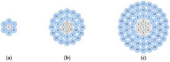
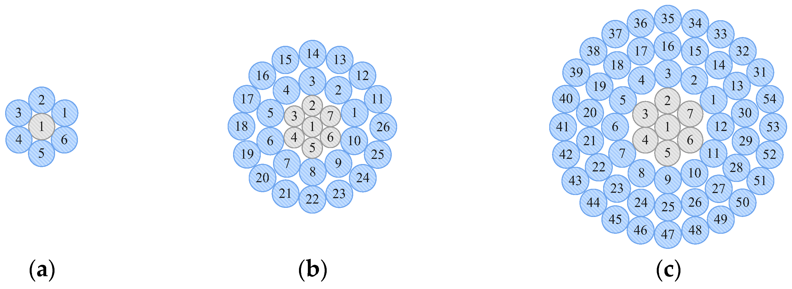
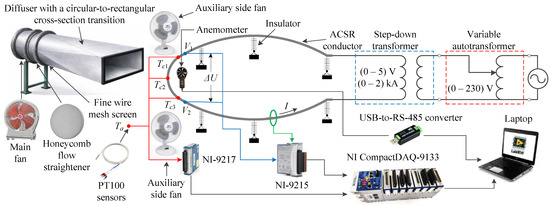
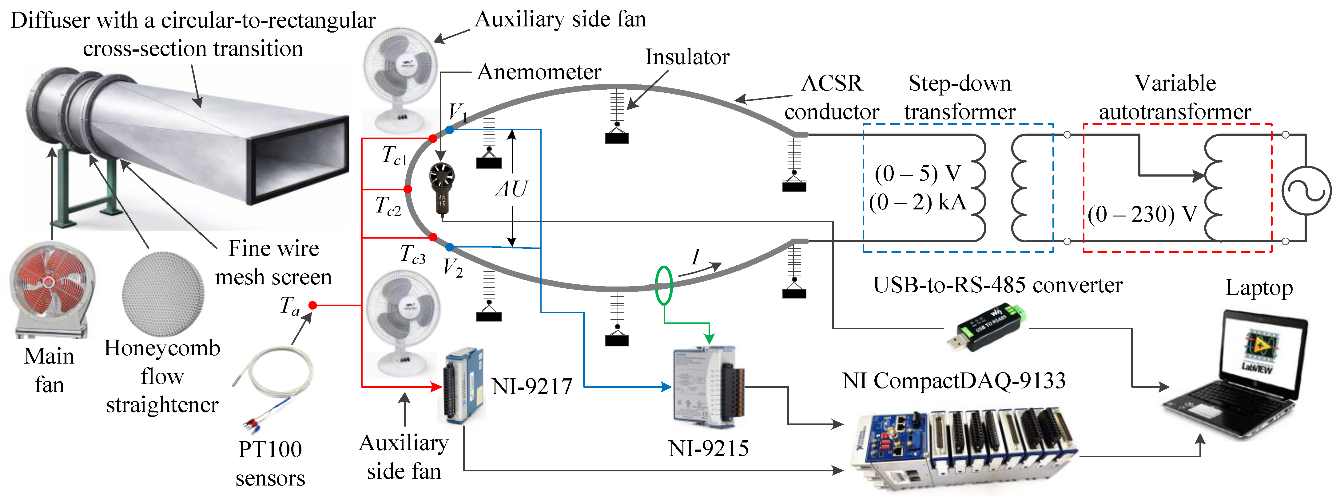
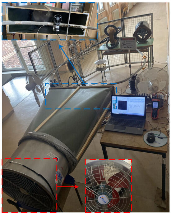
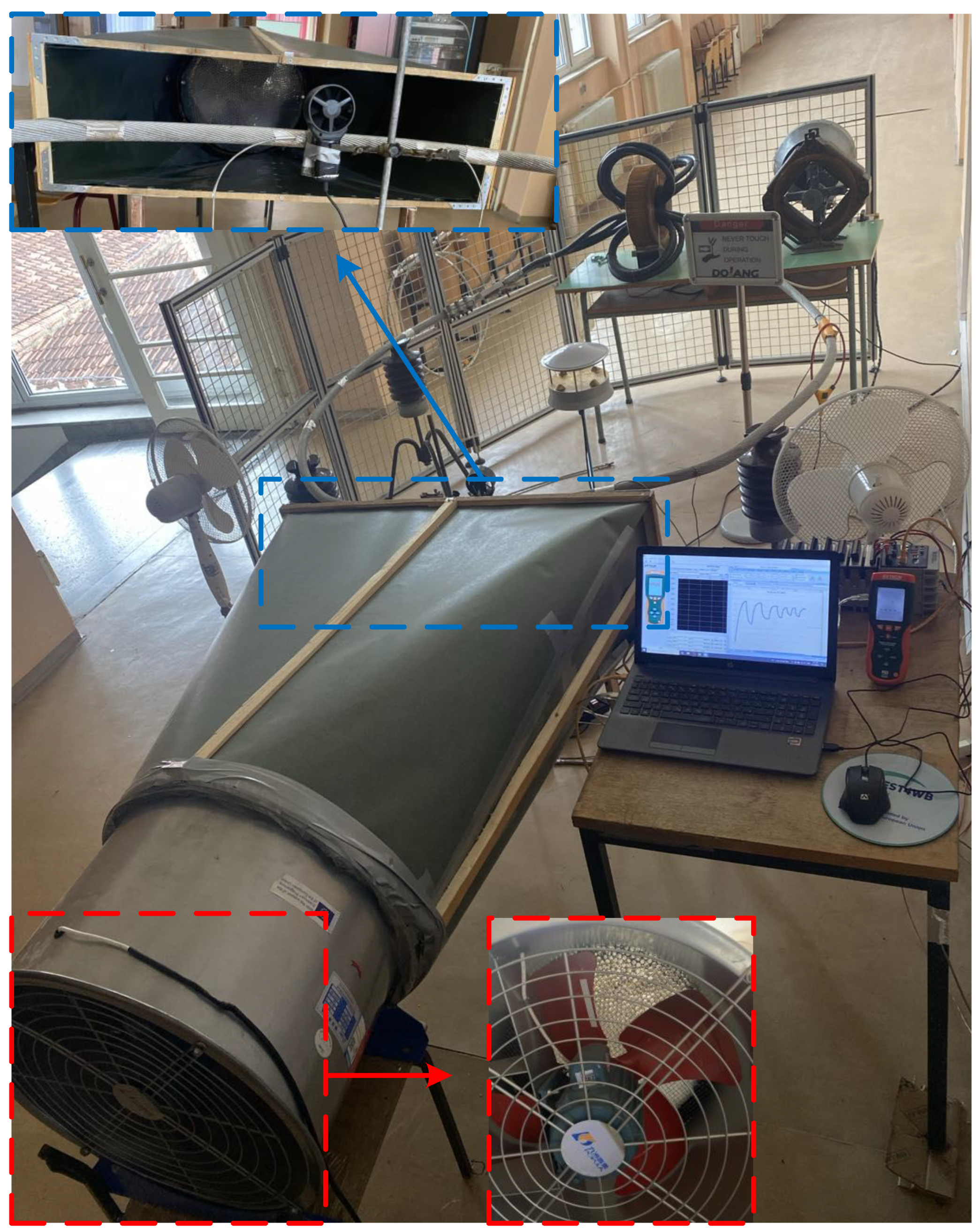
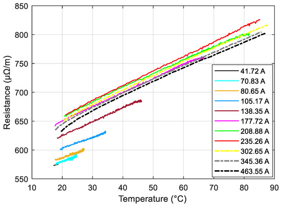
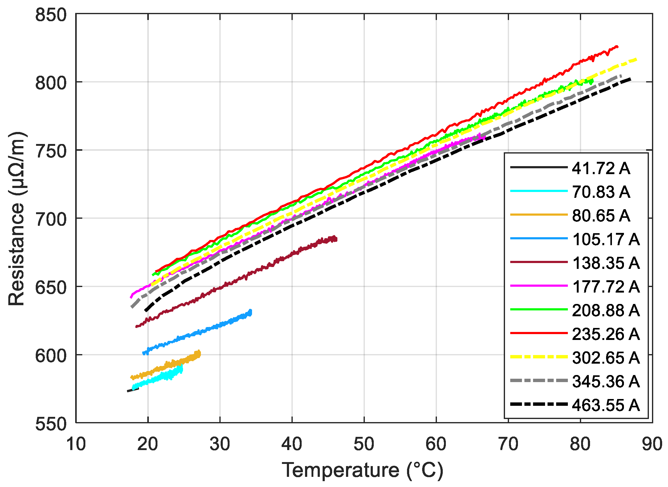
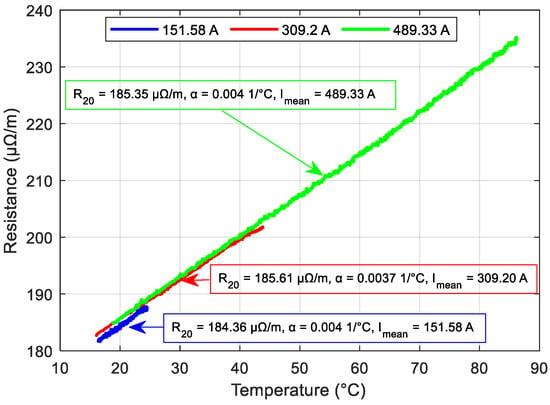
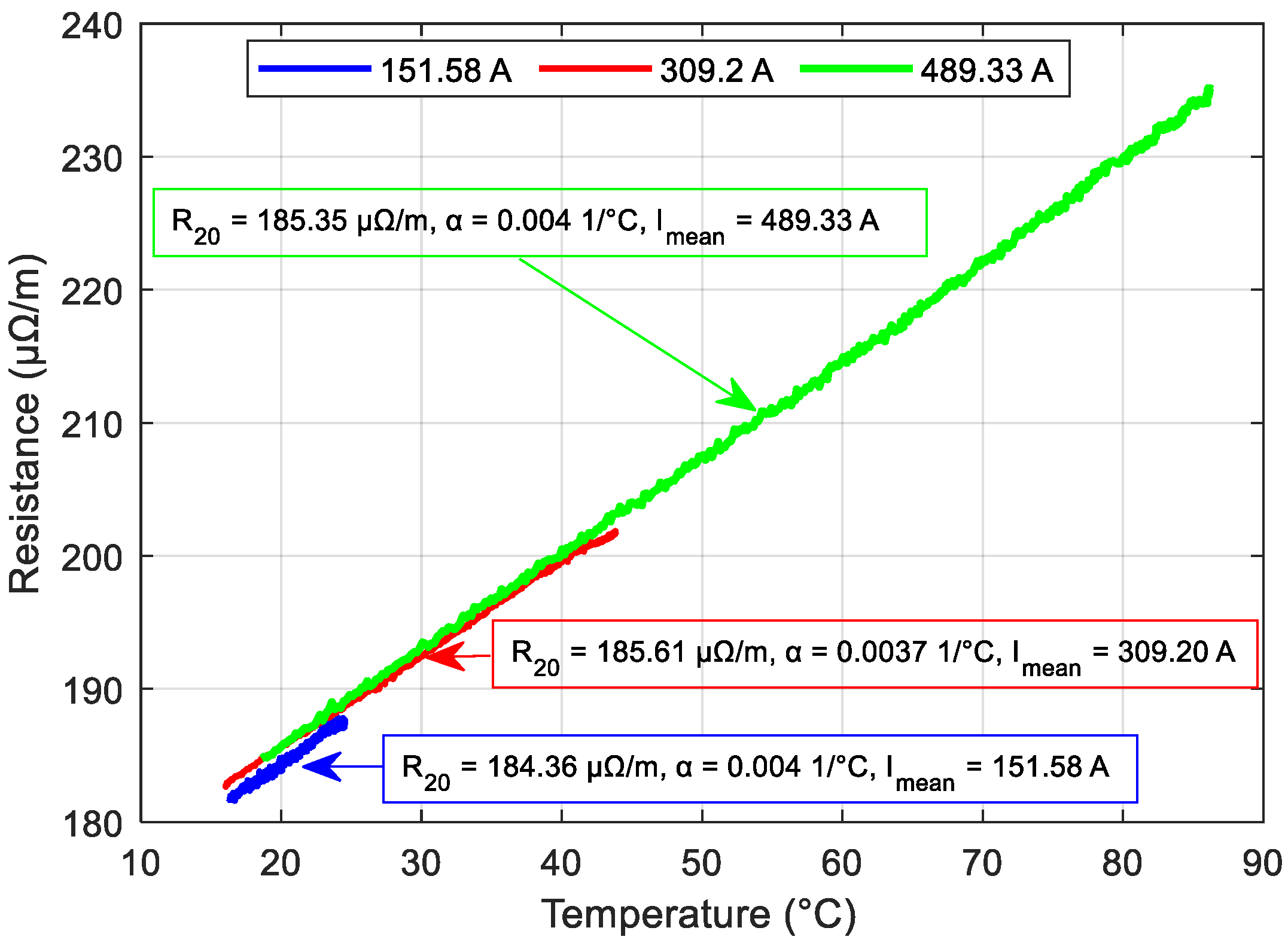
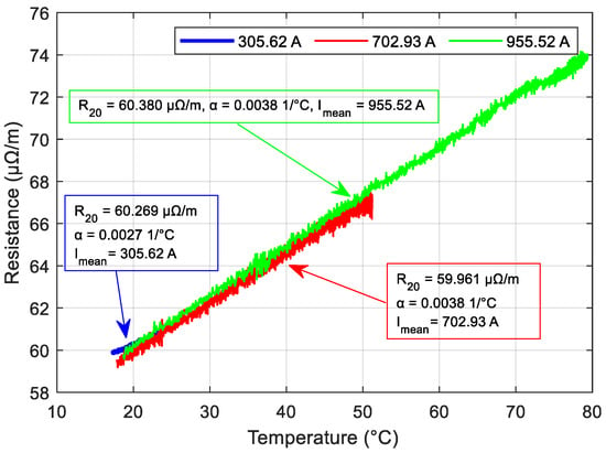
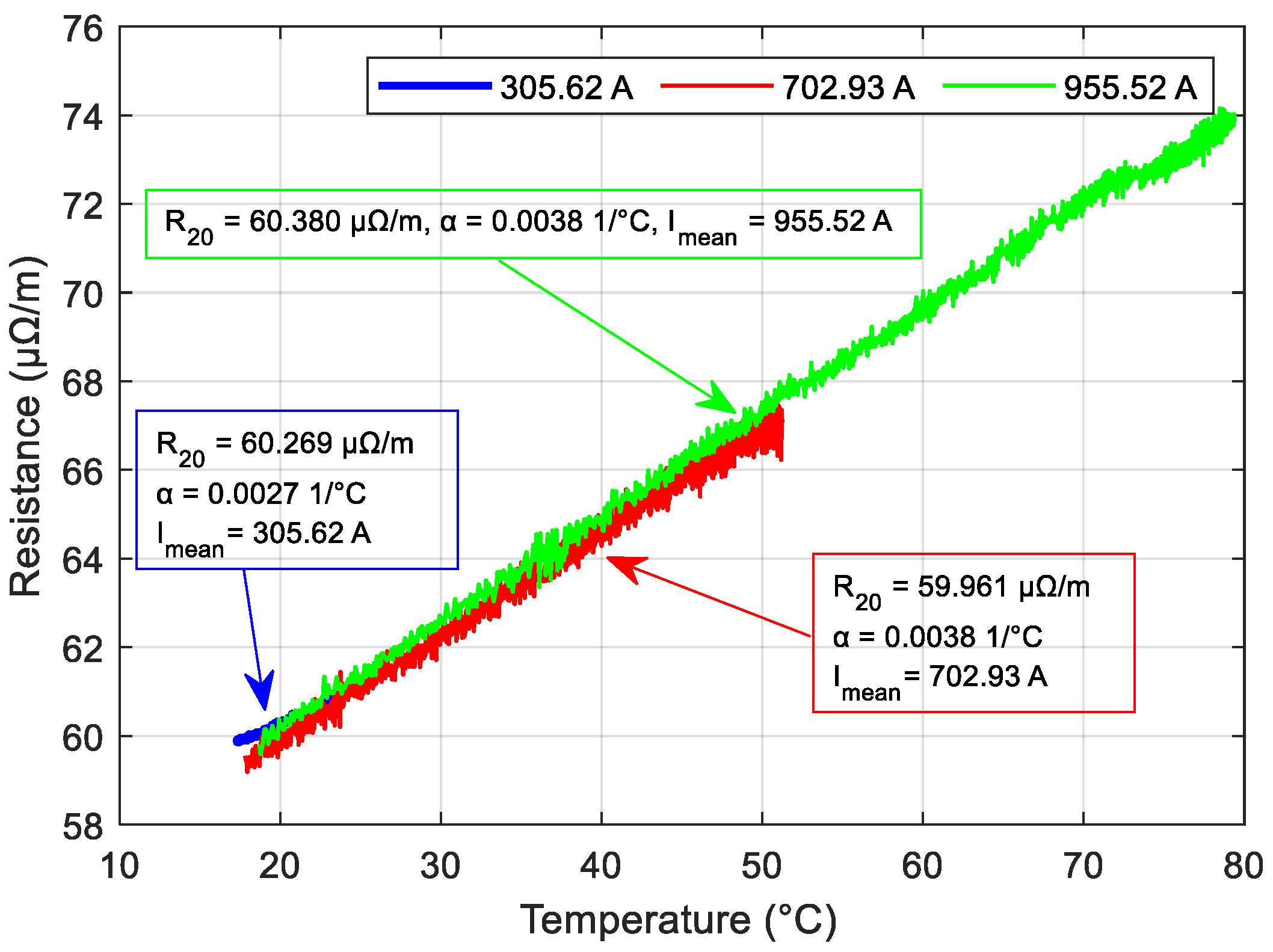
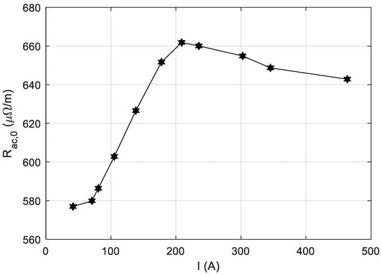
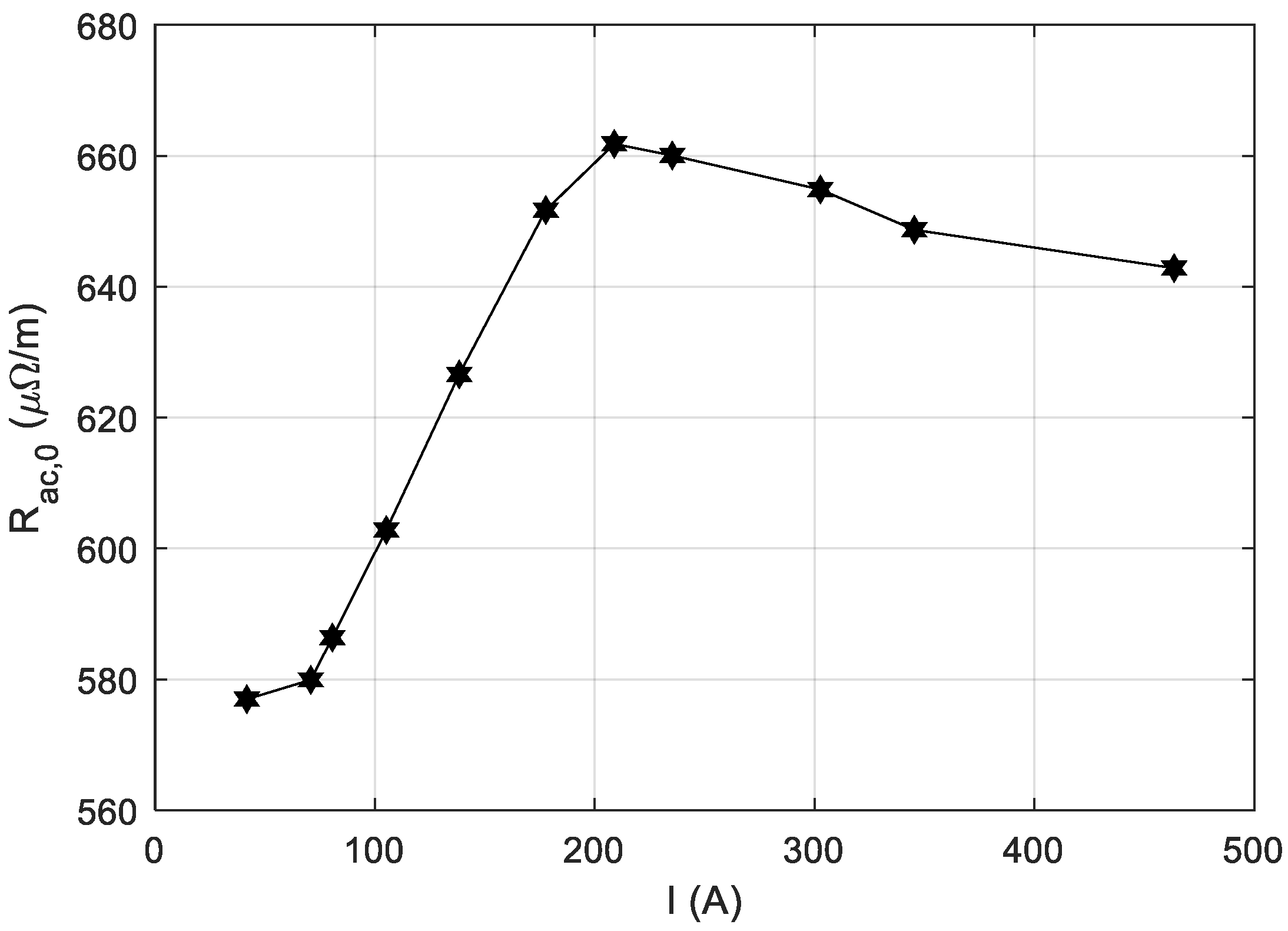
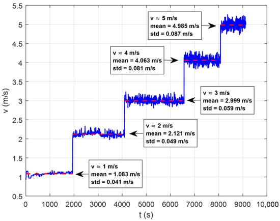
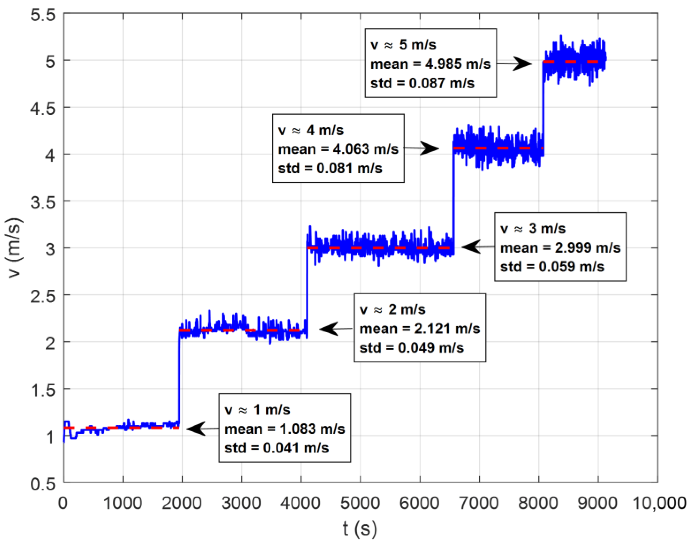
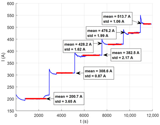
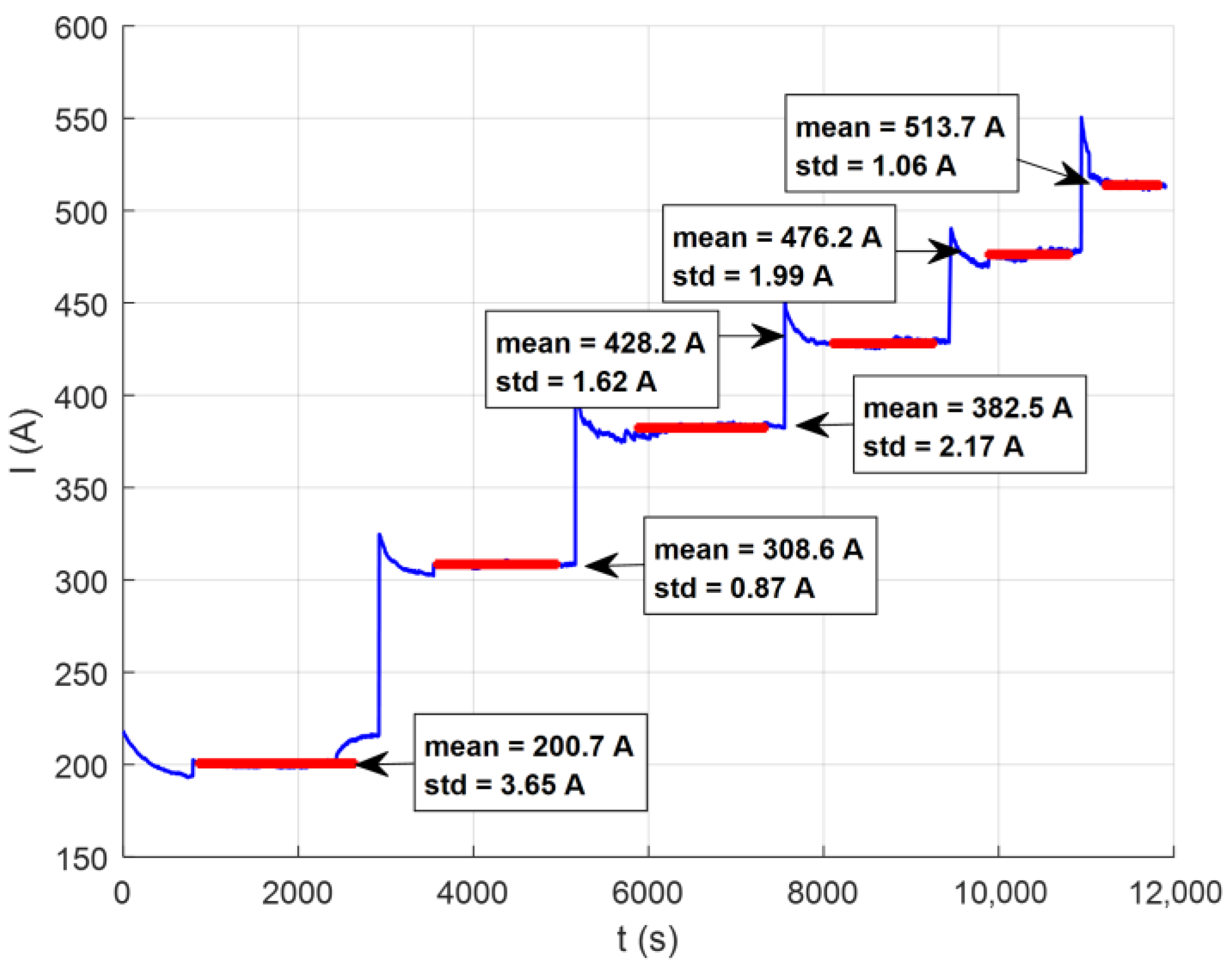
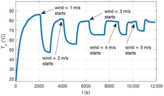
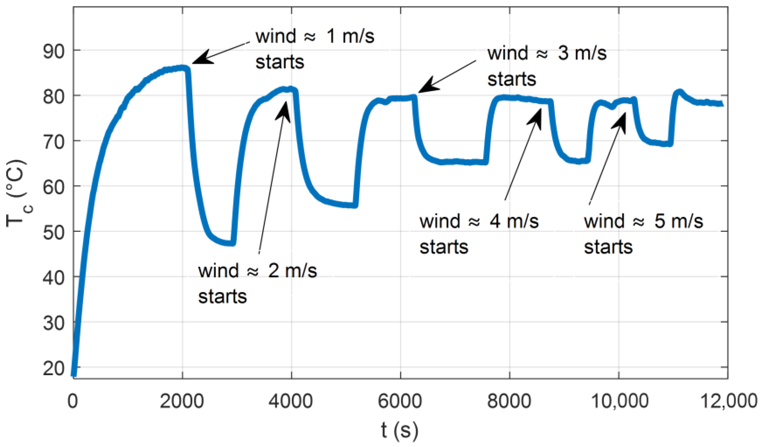
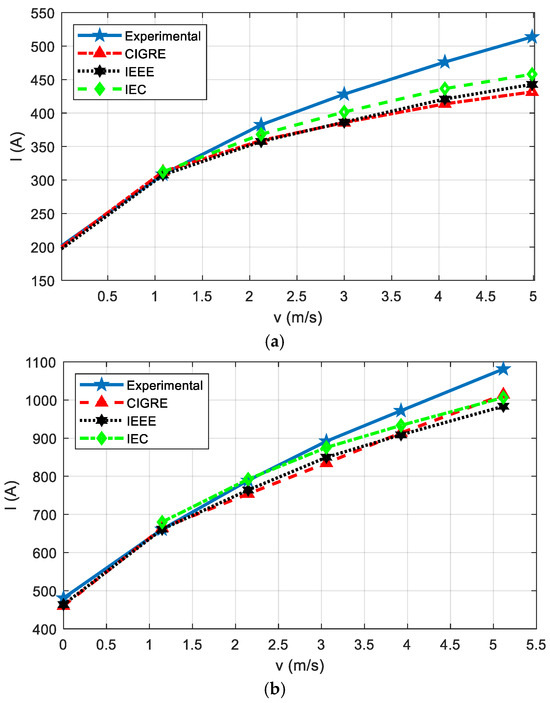
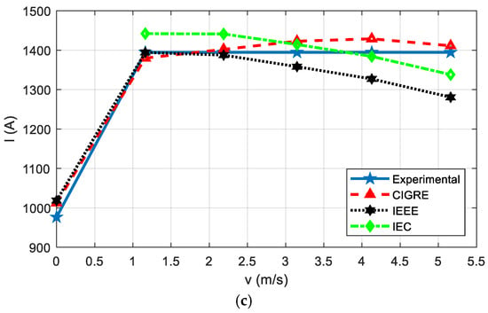
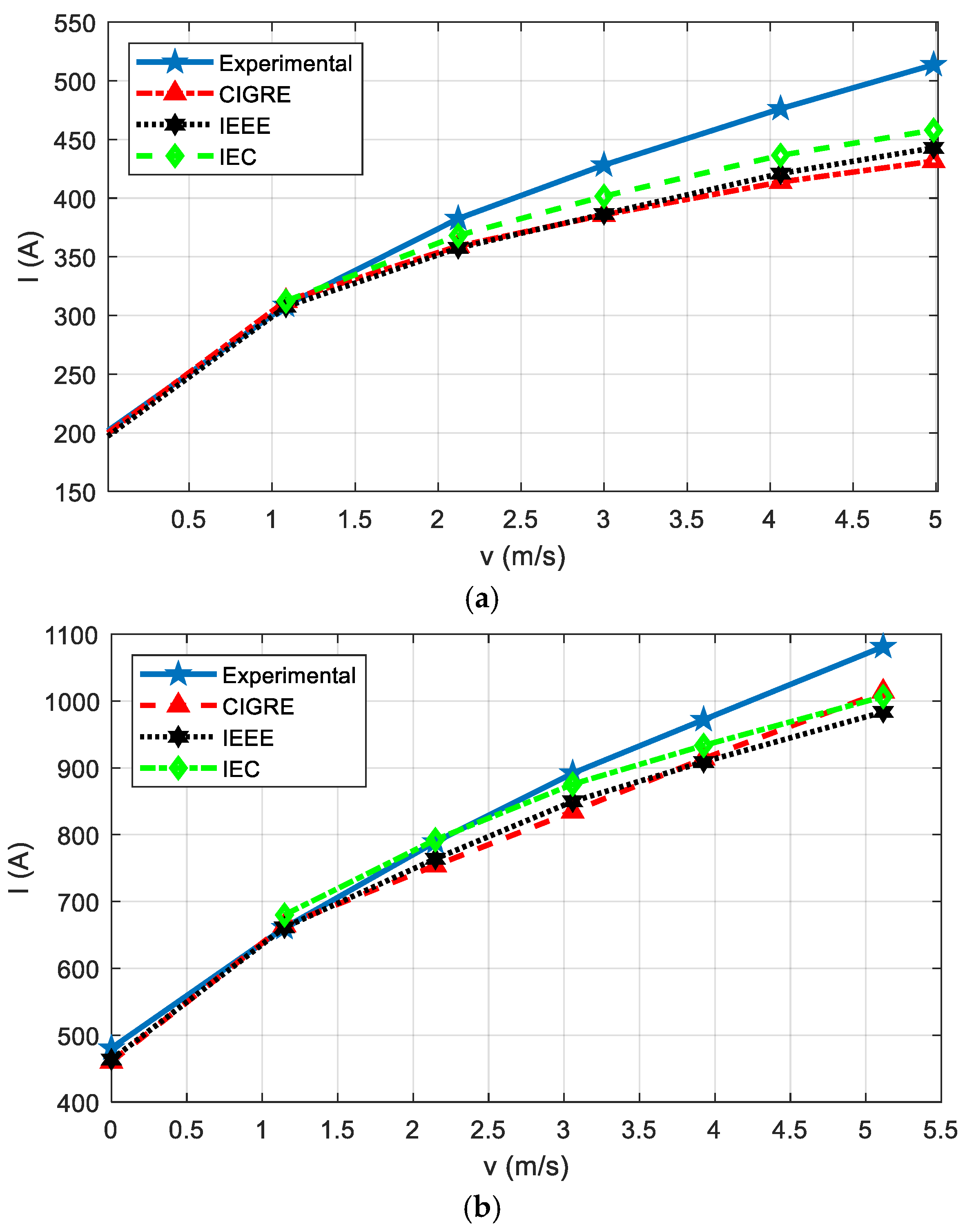
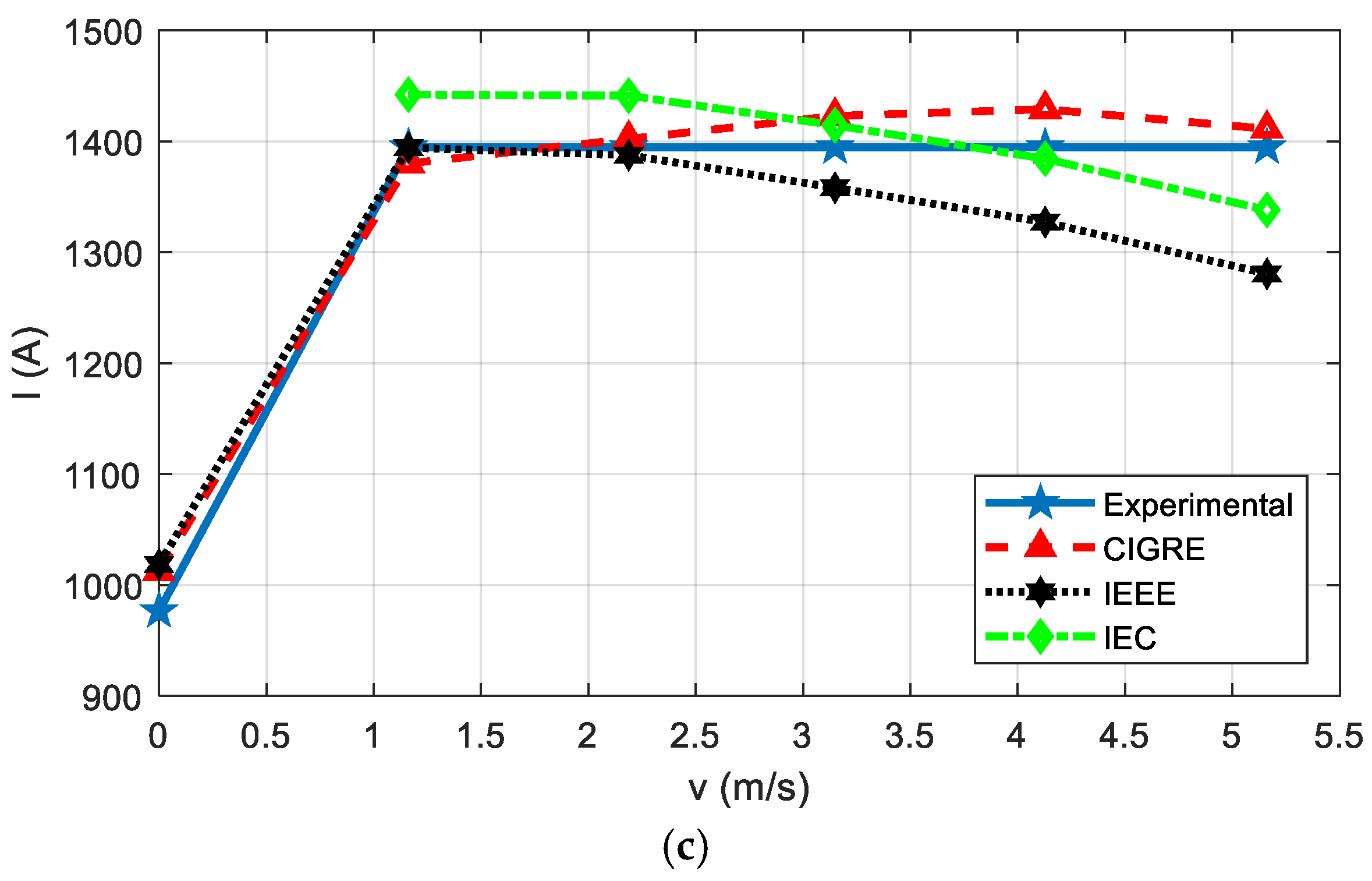
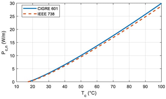
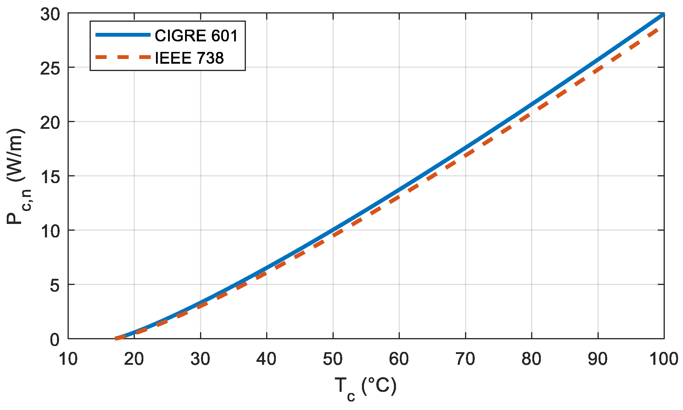
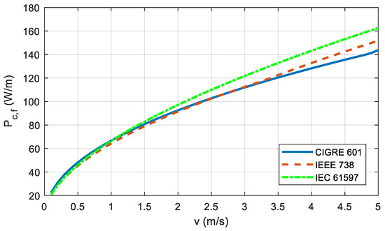
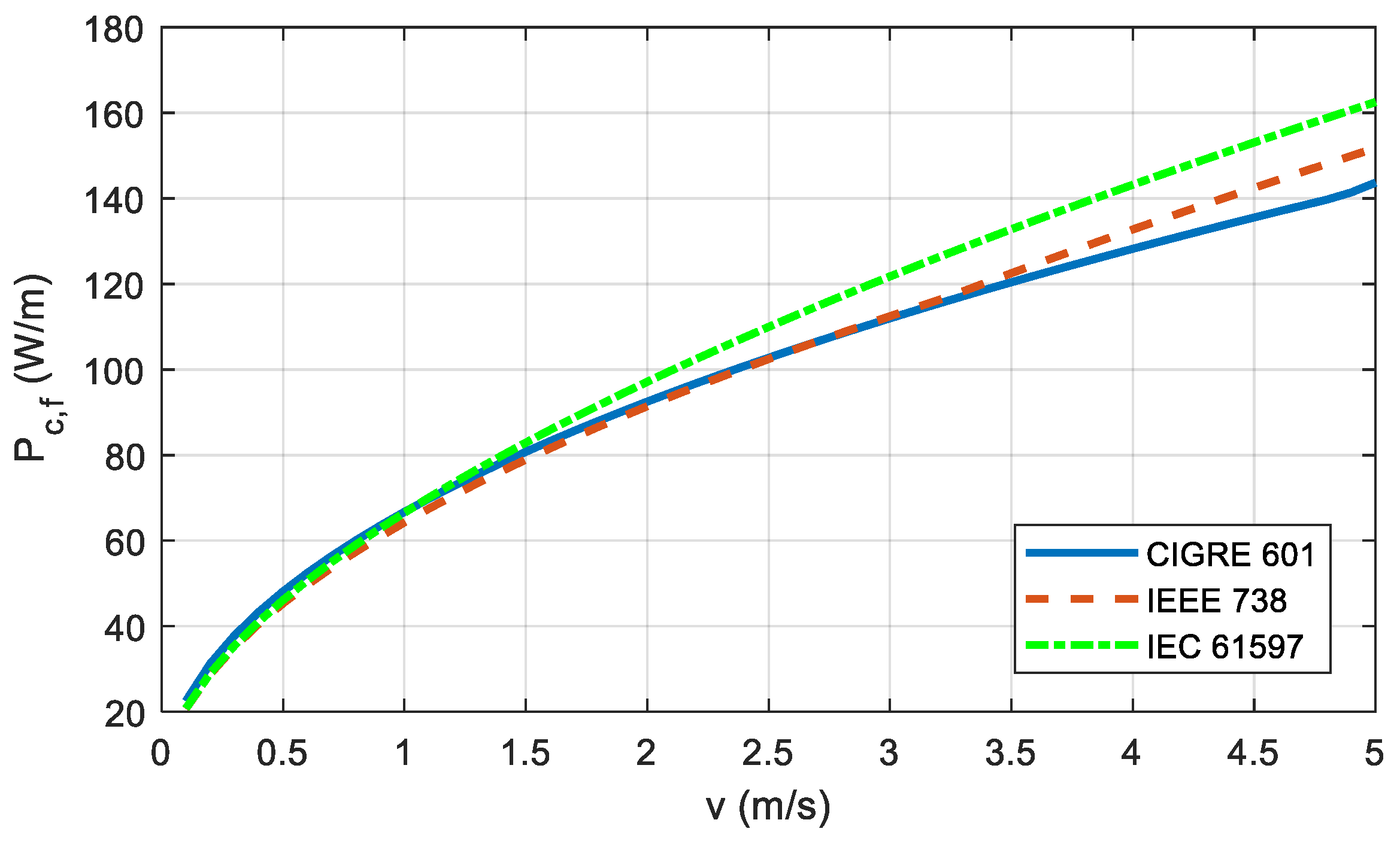
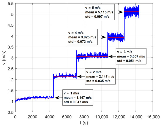
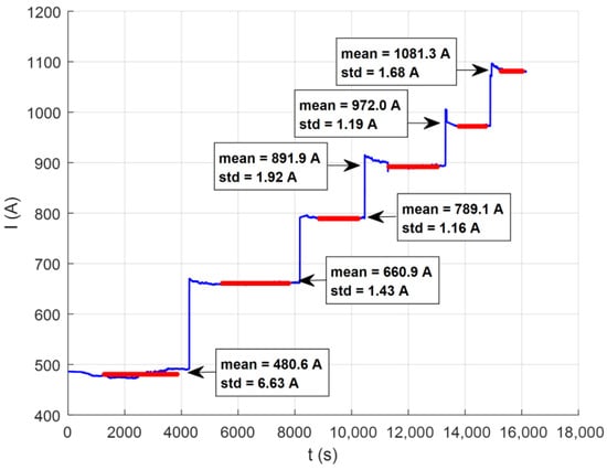
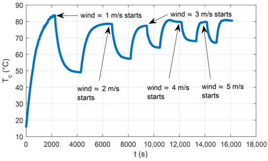
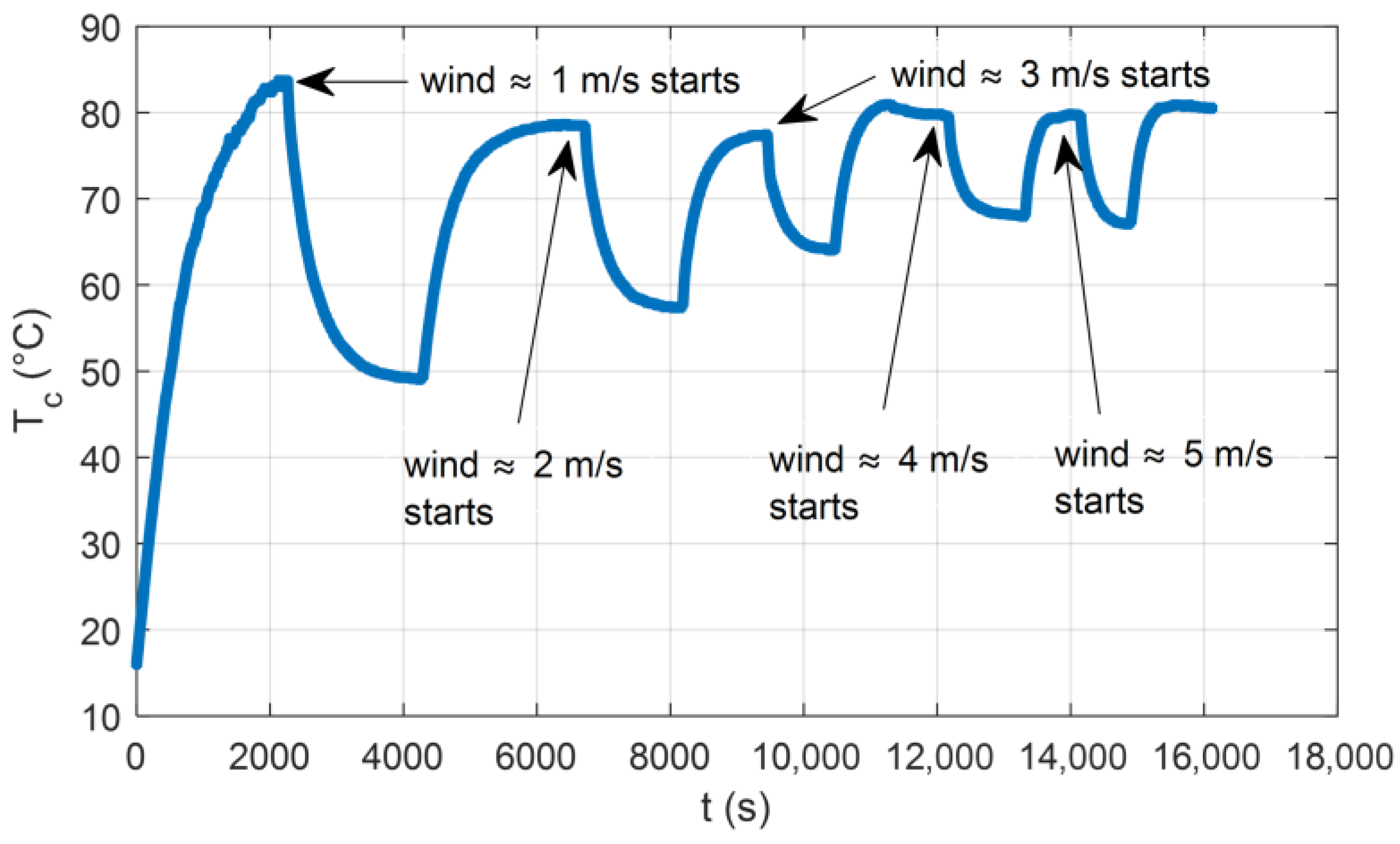
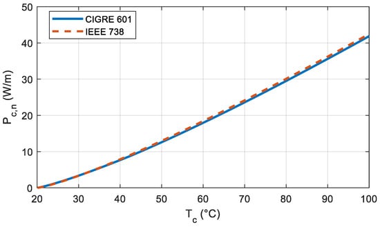
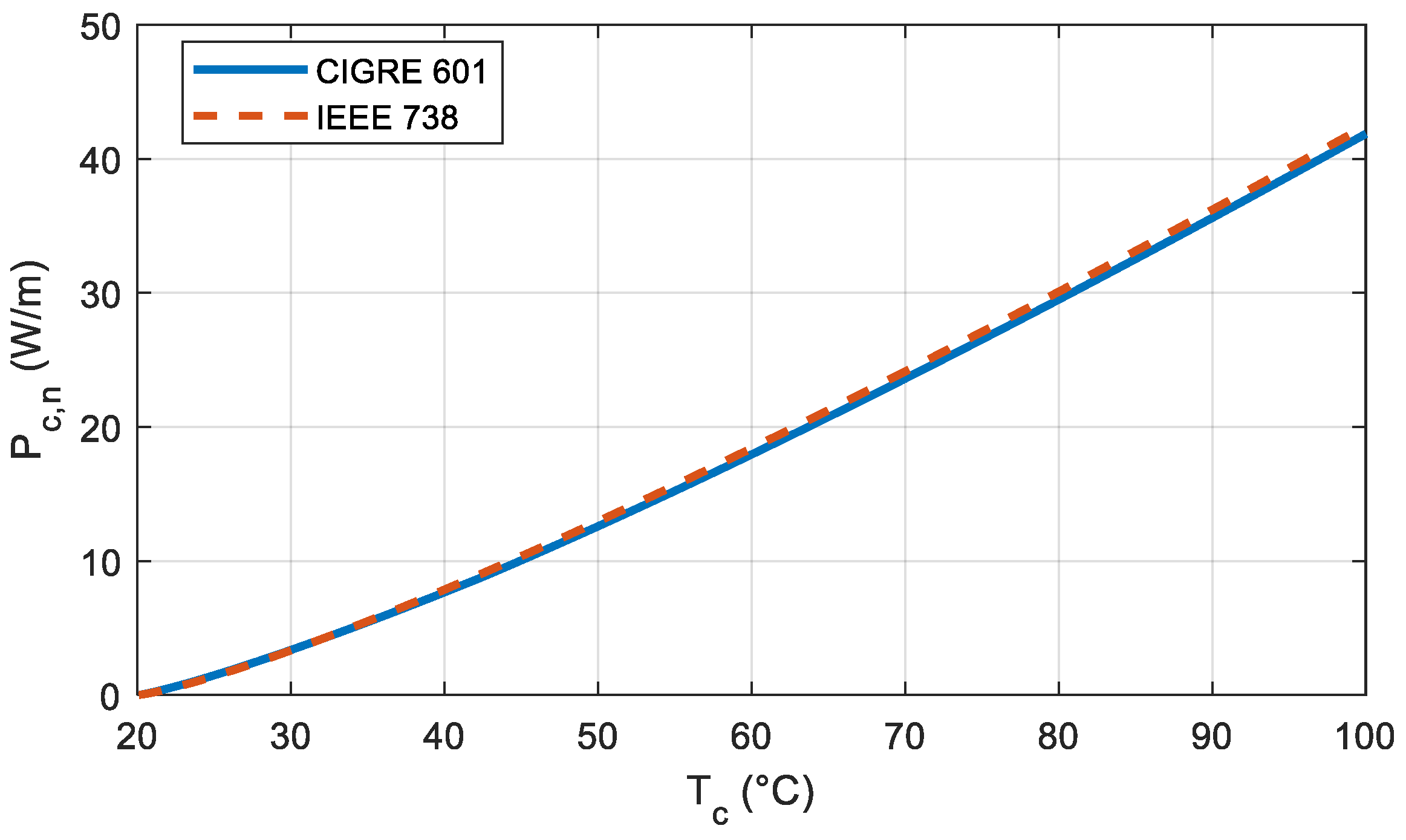
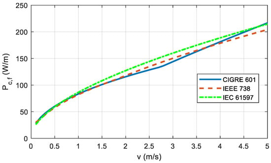
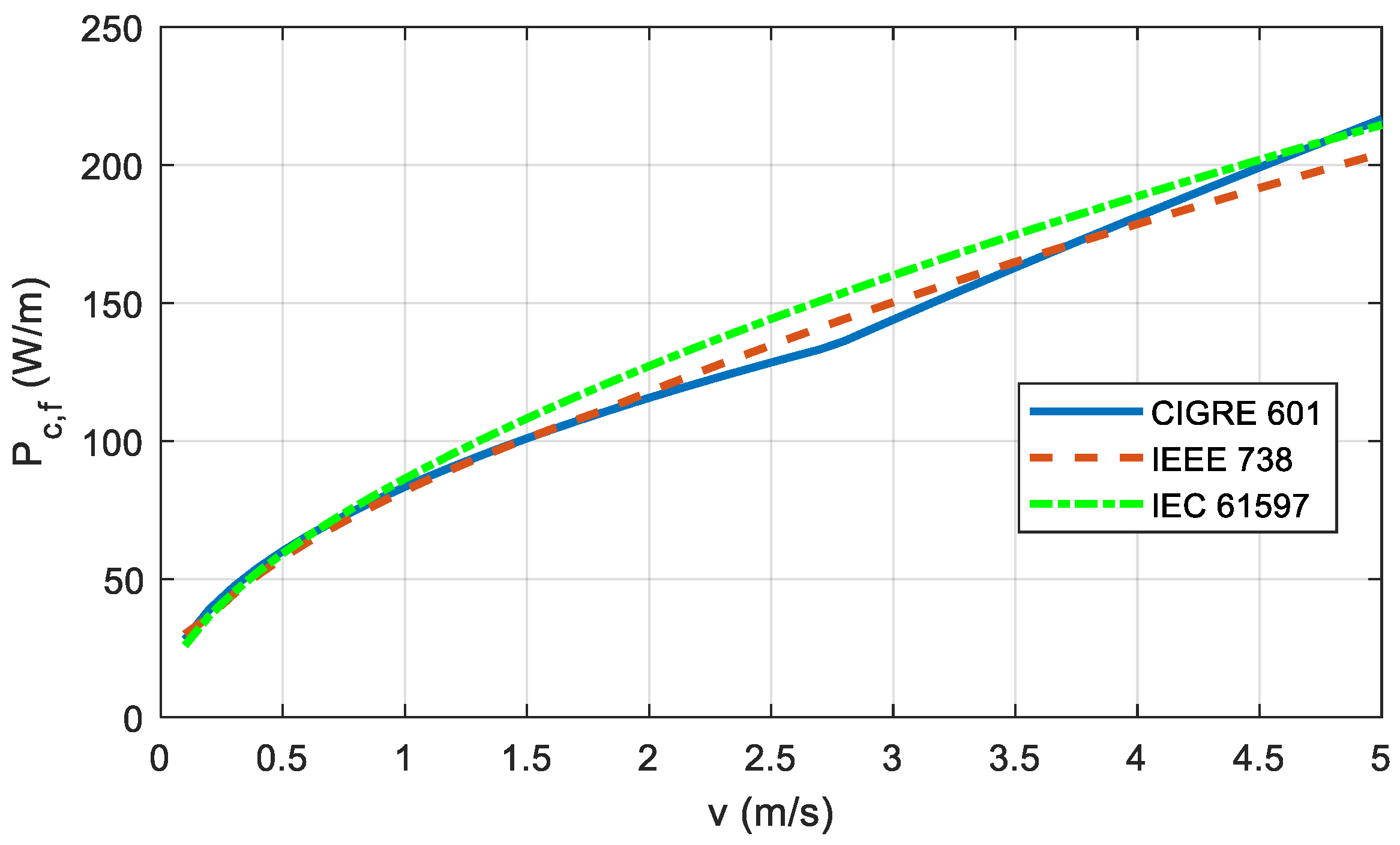
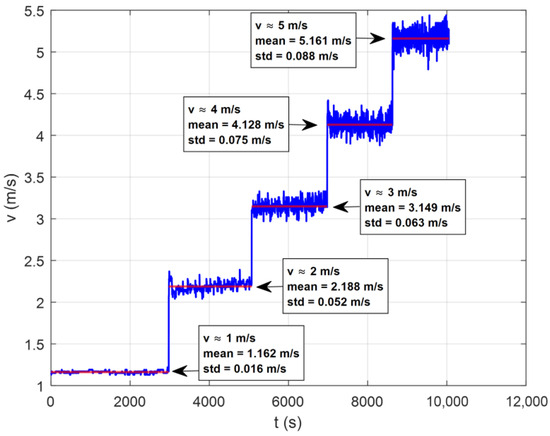
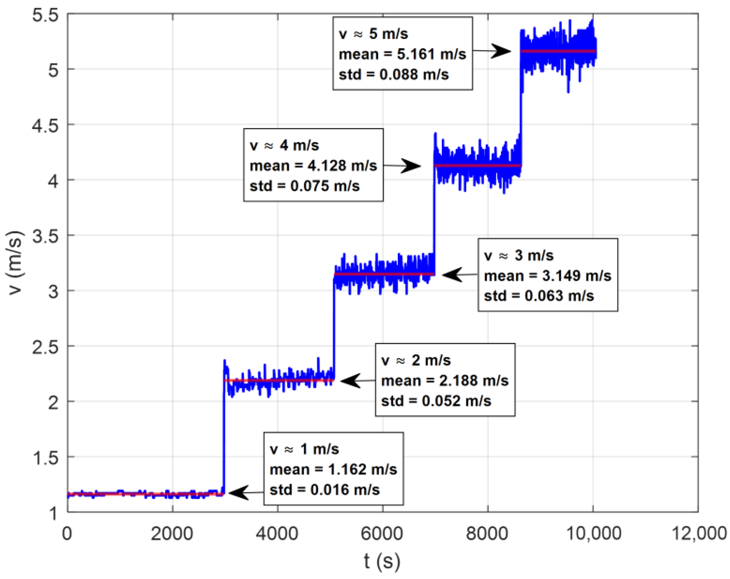
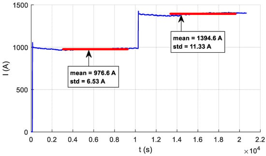
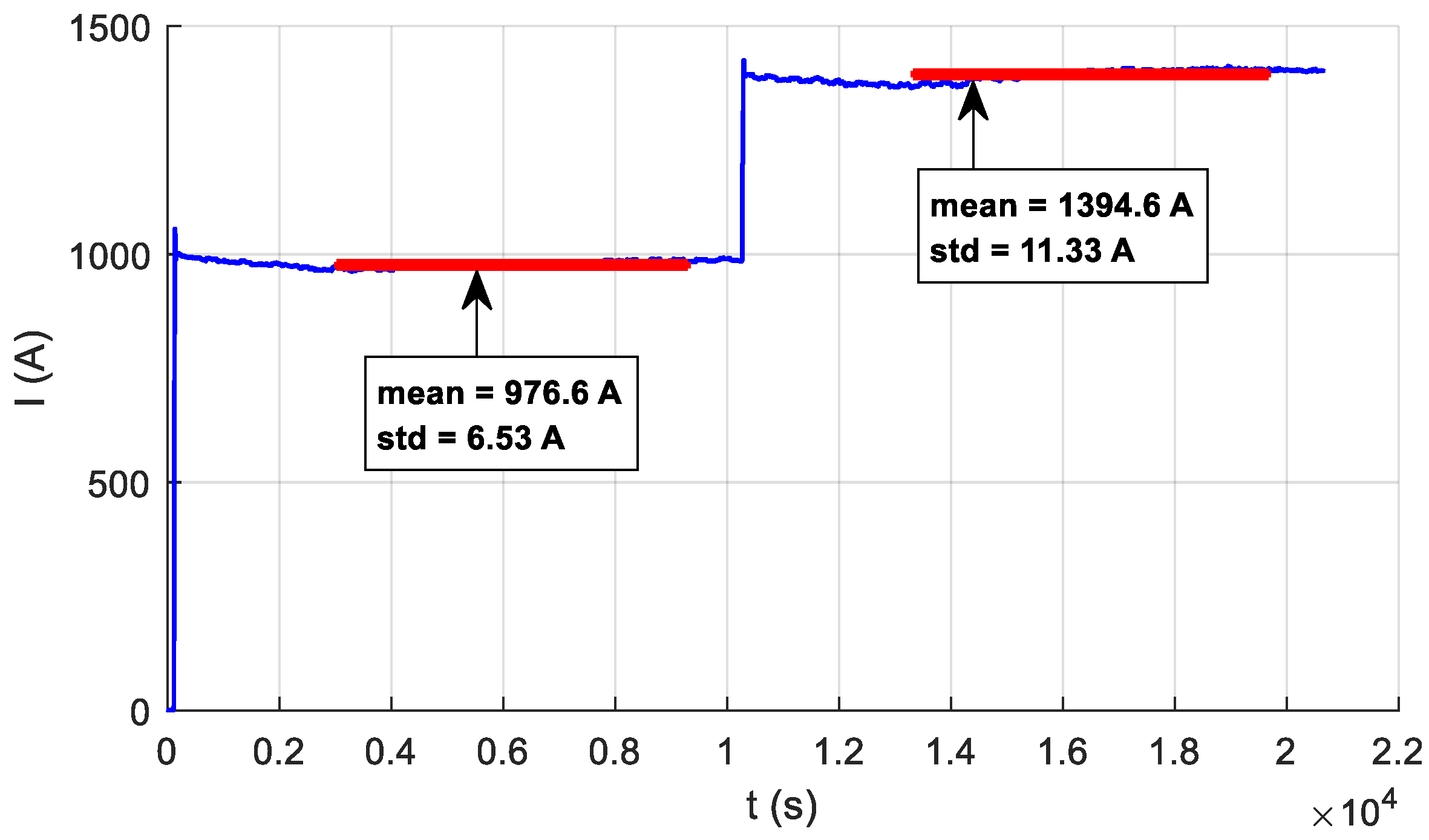
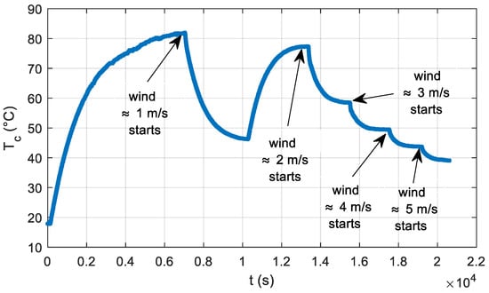
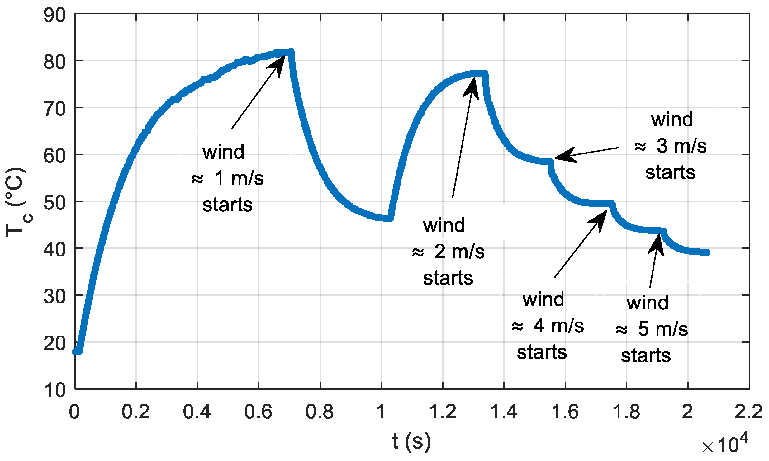
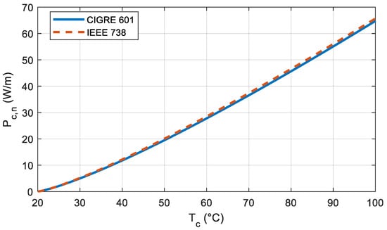
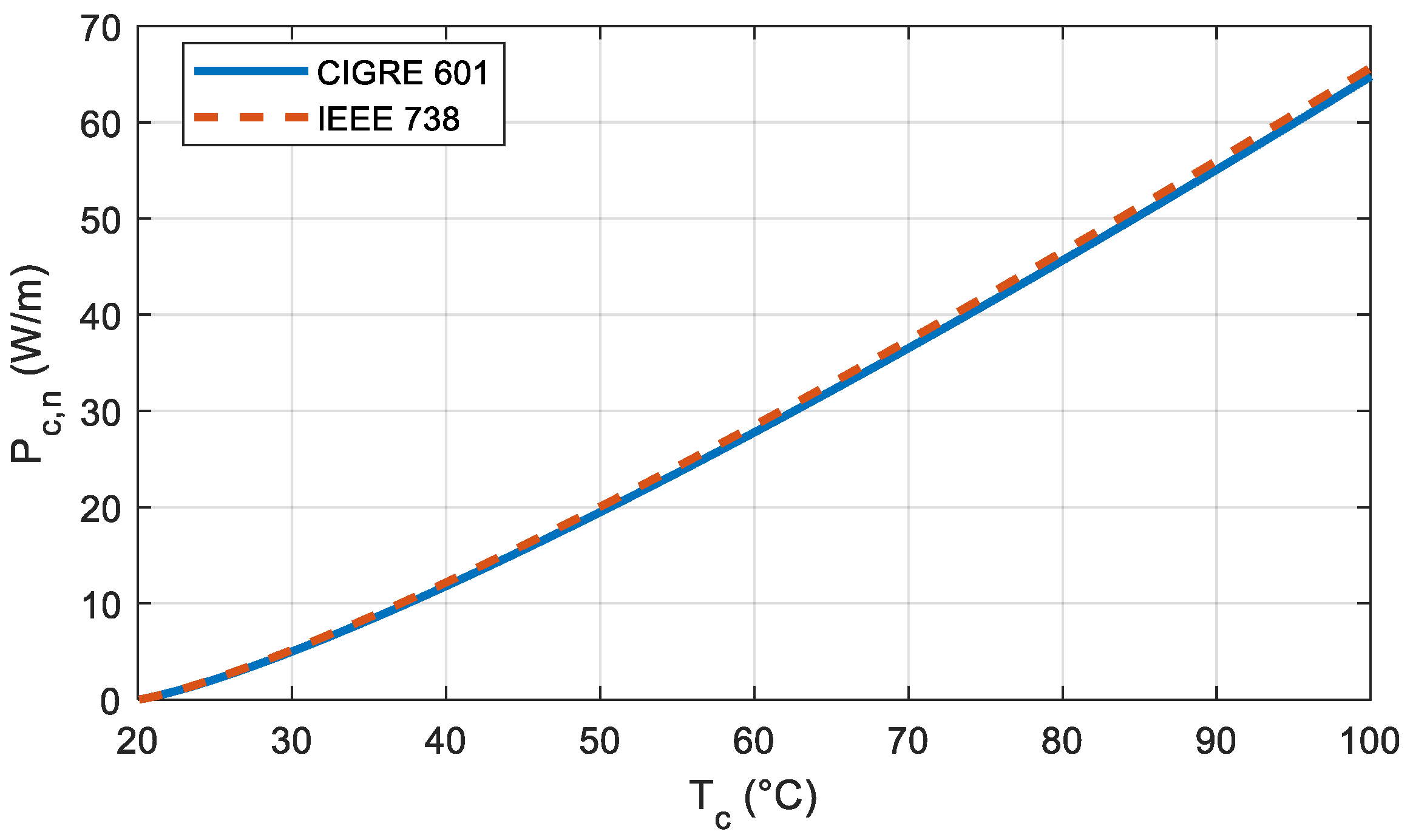
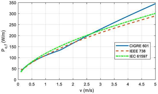
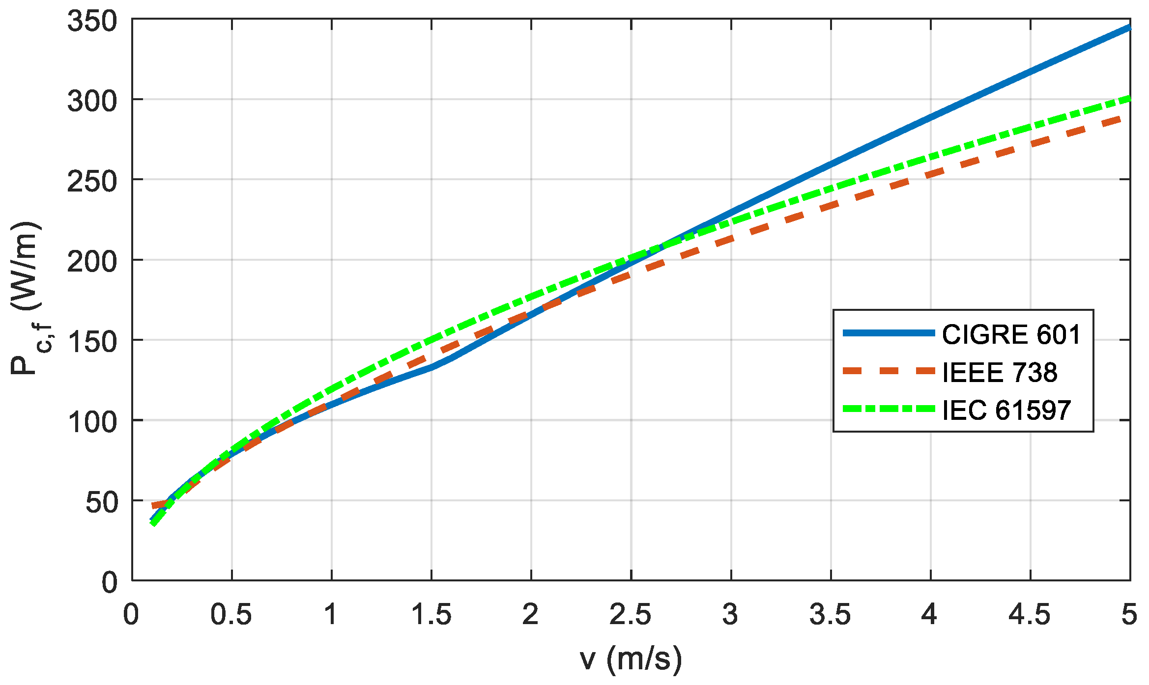

Disclaimer/Publisher’s Note: The statements, opinions and data contained in all publications are solely those of the individual author(s) and contributor(s) and not of MDPI and/or the editor(s). MDPI and/or the editor(s) disclaim responsibility for any injury to people or property resulting from any ideas, methods, instructions or products referred to in the content. |
© 2026 by the authors. Licensee MDPI, Basel, Switzerland. This article is an open access article distributed under the terms and conditions of the Creative Commons Attribution (CC BY) license.