


Abstract
Non-intrusive load monitoring (NILM) can provide actionable feedback for demand response (DR) when direct measurements of device states are unavailable. We propose a reproducible, engineering-oriented pipeline for detecting ON/OFF states of end-use load groups from an aggregated active power time series. The method uses robust hysteresis-based labeling with adaptive thresholds derived from the median and median absolute deviation, followed by compact feature engineering restricted to global active power (GAP). After removing collinear features (|r| > 0.98), permutation importance is used to retain informative predictors. Probabilistic binary classifiers (LGBM, Histogram-based Gradient Boosting, XGBoost, and CatBoost) are trained for each target load, and the decision threshold is optimized via Fβ to balance missed events and false alarms. A post-processing stage stabilizes predictions by smoothing probabilities and suppressing spurious triggers. Model quality is assessed with both sample-wise metrics and event-based metrics that credit the correct detection of switching intervals within a time tolerance. Experiments on the open “Individual Household Electric Power Consumption” dataset (1-min resolution, 2007–2010) demonstrate that lightweight gradient boosting models, particularly LGBM, deliver reliable and interpretable state estimates suitable for practical DR integration and edge deployment.
1. Introduction
One of the ways to improve energy efficiency in power supply systems with low capital expenditure, provided that sufficient load flexibility is available, is demand response (DR) [1]. Demand response, taking into account the classification of electrical loads developed in the authors’ previous studies, enables the application of load-control algorithms depending on the load class; however, stable operation requires feedback on the state of the end-use device and on the load response to the demand-response control signal [2,3].
Such feedback can be provided by integrating the information streams of the SCADA system with the control system of the power supply system [4,5]. However, when this information is not available, recent machine learning and data-processing studies suggest that the state of an end-use device can be inferred using NILM models [6,7].
From a DR perspective, NILM is not only an energy disaggregation task but also a practical mechanism to infer device/group-level operating states when direct device telemetry is unavailable or costly. In such settings, the key requirement is often reliable ON/OFF state (event) detection from aggregated measurements, because actionable DR feedback depends on timely identification of switching events and stable state tracking under noise, multi-device overlap, and measurement constraints [8]. This motivates engineering-oriented pipelines that emphasize reproducibility, limited sensing requirements (e.g., GAP-only), and evaluation protocols that reflect event timing tolerance in addition to sample-wise accuracy.
Numerous studies address non-intrusive load monitoring (NILM) and related load monitoring methods. For example, [9] provides a review of state-of-the-art methods for online NILM in load monitoring applications based on aggregated data. Nevertheless, existing reviews do not sufficiently formalize the requirements for feature causality and for a reproducible protocol for feature engineering workflows.
Recent AI/ML research in NILM has increasingly explored deep sequence models (e.g., CNN/RNN/attention-based architectures), representation learning, and methods aimed at robustness, uncertainty awareness, and generalization under non-stationarity. A complementary line of work emphasizes “trustworthy” energy disaggregation—covering reliability, interpretability, privacy, and robustness considerations—highlighting that deployment constraints and real-world data drift remain major bottlenecks beyond pure predictive performance. In this respect, reference [10] provides a comprehensive review of challenges and perspectives toward trustworthy energy disaggregation and discusses why reproducible baselines and transparent decision logic remain valuable. At the broader smart-grid level, recent surveys summarize how AI/ML methods are used for grid monitoring, stability, and energy-management applications, reinforcing the need to balance model complexity with operational constraints in real deployments [11].
In line with these AI/ML trends, studies [12,13,14] explicitly report the high effectiveness of large language models and multi-task probabilistic network models. However, they also highlight extremely high computational complexity, which constrains implementation on devices with limited computational resources—an important requirement for target industrial and commercial deployments with resource-constrained edge computing [15]. Moreover, in the context of binary classification, the models discussed in those studies are likely to be unnecessarily complex [16].
Therefore, for DR feedback loops that require reproducible behavior and predictable runtime on resource-constrained edge/enterprise platforms, lightweight models paired with transparent feature pipelines remain practically attractive—especially when the goal is binary state/event detection rather than full-scale disaggregation.
Study [14] shows that NILM can effectively analyze energy consumption processes in industrial settings, yielding satisfactory results even with limited datasets. In turn, augmenting NILM with auxiliary methods for dimensionality reduction and clustering has achieved high accuracy (ACC = 95%) in identifying load types, which is required for effective demand response [17]. However, the considered studies do not provide an in-depth analysis of the results using event-based model quality metrics. Primarily, this is because the works do not address the binary classification problem; nevertheless, it should be noted that the direct use of accuracy (ACC) in NILM tasks is not always appropriate.
In [18,19], a reasonable boundary is drawn between the achieved gains in energy efficiency and the energy and computational costs of the developed algorithms. The results can be interpreted as motivation to offload computations associated with heavy machine learning models to remote servers. The classical machine learning models considered in this work (HGB, XGB, LGBM, and CAT) are not resource-intensive for online deployment on an enterprise server, although they may require substantial resources for training [20,21].
This work advances NILM research by proposing a reproducible, engineering-oriented algorithm for inferring end-use device states based on binary classification of an aggregated electricity consumption time series. Unlike most studies focused on pointwise metrics, we introduce and employ event-oriented quality assessment, which is more consistent with demand-response tasks and with monitoring the load reaction to control actions. We show that machine learning methods, with appropriate post-processing and threshold selection, provide stable and interpretable results suitable for practical integration into DR systems.
The study aims to detect the states of individual loads (ON/OFF) from an aggregated electricity consumption signal as a component of the feedback loop in demand-response systems. The aggregate time series is used as the source of features, and the modeling procedure includes data preparation, labeling, feature construction, and training of binary classifiers for each target load.
It should be noted that experimental validation in this work is performed using an open residential electricity consumption dataset. This dataset was selected due to its representativeness, its time resolution relevant to demand response, and the availability of labeled end-use load groups, enabling reproducible comparison of load state-detection methods.
2. Materials and Methods
2.1. Dataset Description
This study uses the open dataset “Individual Household Electric Power Consumption” [22]. The dataset is provided as a CSV file containing 2,075,259 measurements collected in a private house located in a suburb in France over the period 2007–2010. The sampling interval is 1 min. The overall fraction of missing values is 1.25%.
The raw data comprise four main time series synchronized in time: the household-wide electricity consumption series, and three electricity consumption series corresponding to individual end-use load groups.
The first end-use load group (Sub_metering_1) exhibits no clear periodicity and occasional low-magnitude consumption spikes. The Sub_metering_1 measurements were obtained on the feeder supplying selected kitchen appliances.
The second end-use load group (Sub_metering_2) is characterized by periodic switching and relatively small magnitude compared with the household total (peak power of about 2 kW versus a peak aggregated household demand of about 32.5 kW). The Sub_metering_2 time series represents loads located in the laundry room.
The third end-use load group (Sub_metering_3) demonstrates stable periodicity and a high amplitude relative to the household total. This subgroup corresponds to the boiler room and includes several large consumers, such as a water heater and an air-conditioning system.
Notably, the metering system does not cover all consumers. According to summary statistics, the coverage ratio is CR = 48.8%. In this study, this limitation is beneficial because it introduces an additional unmetered component that better approximates real-world conditions. The coverage ratio was calculated as:
where —is the total energy recorded by the n-th sub-meter over the period considered (kWh), and —is the total household electricity consumption over the same period (kWh).
2.2. Algorithm Description
Solving the binary classification problem using machine learning (ML) methods in the context of equipment-state monitoring can be reduced to the following five stages:
- Data loading and basic transformations (Step 1);
- State labeling and dataset construction (Step 2–5);
- Model training (Step 6);
- Threshold selection and repeated validation (Step 7–8);
- Final visualization and export of results (Step 9).
The methods used at each step are described below, starting from Step 1. At the first stage, the data are loaded and the time series corresponding to total household electricity consumption and to candidate predictors are identified. Basic transformations include harmonizing the scale of the electricity consumption data: sampling interval of 1 min and energy units initially expressed as , which were converted to the conventional form for subsequent calculations. During preprocessing, missing values in the time series are imputed using time interpolation combined with limited value propagation, which provides a more physically meaningful signal reconstruction than linear interpolation or mean imputation.
After preprocessing, Step 2 forms additional predictors and, in particular, generates state labels for electrical loads. State labeling is based on the hysteresis principle. The hysteresis labeling method converts a power time series into a binary state sequence using hysteresis with adaptive thresholds computed from the median and the median absolute deviation (MAD), with filtering of short-duration false triggers. Hysteresis labeling built on robust statistics represents a hybrid of physical and statistical approaches and, in essence, constitutes an adaptive time series segmentation using non-linear thresholds. It does not rely on a priori device characteristics; instead, it exploits properties of the signal itself.
Let denote the target sub-metering power time series used to construct proxy ON/OFF labels. We compute robust location and scale estimates on the calibration window as:
where prevents division-by-zero. The adaptive hysteresis thresholds are then defined as:
with . The state is updated causally: the label switches from OFF to ON when and switches from ON to OFF when .
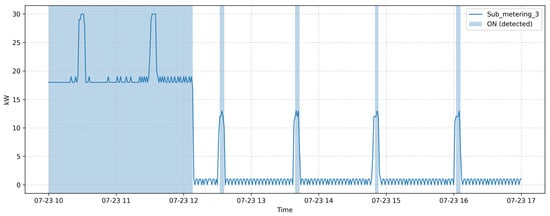
The results of hysteresis labeling for a data segment are shown in Figure 1.
Figure 1.
Original electricity consumption time series and hysteresis labeling results.
Figure 1 shows that low-amplitude signal components (standby electricity consumption) are not marked as an “ON” state of the load. At the same time, the “ON” label is assigned throughout the entire operating cycle of the load, regardless of whether electricity consumption is constant or varies over time.
To suppress short-duration false triggers, we apply two causal duration rules. First, an OFF to ON transition is accepted only if the condition holds for at least consecutive samples (minutes), where is target-specific. Second, after probability thresholding, we apply a morphological post-processing to the predicted binary mask: ON segments shorter than are removed (set to OFF), and OFF gaps between two ON segments are filled if the OFF gap length is .
At Step 3, after labeling, the original dataset is enriched with a set of statistical features. At this stage, a set of features suitable for machine learning is extracted from the DateTime time stamps. The purpose of this step is to transform the raw data into a feature space in which the difference between the “ON” and “OFF” states becomes linearly or quasi-linearly separable.
In the proposed algorithm, feature construction is centered on a single aggregated parameter—global active power (GAP). The derived predictors are referred to as GAP features according to their origin. The measured active power P(t) reflects the total electricity demand of all devices. Temporal, amplitude-based, and derivative characteristics are extracted from P(t) to describe load dynamics. The algorithm constructs three groups of features:
- Instantaneous statistical characteristics: power values, their logarithms, normalized deviations from the median, and local variance. These features characterize the current state of the system.
- Temporal characteristics: moving averages, exponential smoothing, differences between adjacent samples, and the ratio of the current value to a windowed mean. These features capture the rate of change and the transition patterns between states.
- Context features: time of day, day of week, and public holidays. These variables represent the cyclicity of household processes, improving model generalization.
A key feature of this study is the deliberate reduction of the feature space dimensionality. Features are not constructed from the full set of physical parameters available in the raw dataset (voltage, current, etc.) but exclusively from active power. This design choice is motivated by the hypothesis that, for state-detection tasks (as opposed to identification of specific appliances), excessive feature dimensionality does not improve classification performance but increases the risk of overfitting. The resulting feature vectors are augmented with the binary label vector that represents the load state and was obtained at the previous step.
After obtaining the complete feature table, Step 4 performs the removal of collinear features, i.e., predictors that exhibit strong linear dependence on each other. Collinearity implies that a subset of features effectively duplicates information already contained in other predictors [23]. This increases model instability (small perturbations in collinear features can lead to substantial changes in feature weights) and may reduce interpretability, because the model distributes importance across correlated variables in an arbitrary manner. In the proposed algorithm, collinearity is mitigated by computing the correlation matrix for all features and removing redundant predictors with high pairwise correlation (|r| > 0.98). Sensitivity at threshold |r| will be tested further in Section 2.4. From each strongly correlated group, one feature is retained, eliminating duplicated information and reducing dimensionality without sacrificing predictive power.
Unlike the dimensionality reduction performed at the previous stage, Step 5 selects features based on their predictive value. Feature importance is computed using repeated training of a Histogram-based Gradient Boosting (HGB) model, followed by permutation of each feature and evaluation of the performance drop measured by average precision (AP). This further reduction in feature dimensionality decreases the probability of overfitting, which is particularly important under class imbalance (e.g., Sub_metering_2 contributes far less than Sub_metering_3).
All experiments use strictly chronological (time-ordered) splits with no shuffling. For a given training duration and validation duration , the training window is defined as , and the validation window is the immediately following contiguous segment . Feature selection, model fitting, probability calibration, threshold optimization, and all hyperparameter choices are performed using training data only (and, when applicable, a calibration sub-window carved from the end of the training period). Reported validation metrics are computed exclusively on the subsequent validation window.
Unless explicitly stated otherwise, the primary benchmark results (Table 1, Table 2 and Table 3, ROC/PR curves) use days and days. The varying validation horizons (3/5/7 days up to one year) and the longer validation horizons (30/60/90 days up to three years) are used only in the training horizon sensitivity study shown in Section 3.2; all these splits remain strictly chronological and anchored at the same starting time .
Table 1.
Differences between metrics.
Table 2.
Differences between metrics in different threshold.
Table 3.
Sensitivity to the permutation importance procedure.
At Step 6, the resulting feature table after primary filtering is used to train the classifier. The key objective of this stage is to build a statistical model capable of predicting, from the feature representation of the current power-network state, whether the device in a given load group (Sub_metering_1–3) is on. The problem is formulated as a binary classification with probabilistic output. Specifically, each candidate model receives a feature vector and produces an estimate of the probability that the device is on,
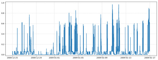
An example output at this step is shown in Figure 2, which presents the predicted probability of the “on” state for the target load within Sub_metering_1 obtained using only the selected GAP features.
Figure 2.
Probability of the “on” state for Sub_metering_1.
At Step 7, a binarization threshold is selected in relative units (or percent). The binarization threshold, denoted , is required to convert probabilities to binary outputs (ON/OFF):
Threshold selection is performed using precision–recall analysis, as shown later in the metrics subsection. To determine a rational threshold, the score is computed. Clarity, precision, and recall are defined as:
which quantifies the fraction of predicted positive instances that are truly positive, and
which quantifies the fraction of true positive instances that are detected by the algorithm. TP, FP, FN, and TN denote the standard confusion-matrix counts. Let P and R denote precision and recall, respectively. The general form of the score is
where controls the relative weight of recall versus precision. For recall is prioritized (missing events are penalized more strongly, at the cost of more false positives), whereas for precision is prioritized (a more conservative model that may miss true ON intervals).
To mitigate class imbalance (especially for the laundry group), all classifiers are trained using class-balanced sample weights computed on the training window. In addition, the decision threshold is optimized using a target-specific ; for the most imbalanced target (laundry) we use to penalize false positives more strongly under rare-event conditions
The score is a weighted harmonic mean of precision and recall; values closer to 1 indicate better performance. The threshold is selected to maximize for the considered values [24].
Next, Step 8 performs post-processing of the resulting binary masks for each load group. A binary mask is a discrete indicator function of the load state obtained by thresholding the probabilistic model output , where corresponds to the ON state and to the OFF state.
Post-processing suppresses spurious triggers caused by sudden probability spikes and eliminates short OFF gaps within the probability time series. Here, is the calibrated ON probability, is the decision threshold, and W is the smoothing window length (min). This stage also includes temporal stabilization of the probabilistic output. Probability calibration is performed using isotonic regression fitted on a dedicated calibration sub-window carved from the end of the training period (chronological split; no shuffling), and the resulting calibrated probabilities are then smoothed using a moving average window W prior to thresholding and post-processing. Specifically, a moving average with window width W minutes is applied to the calibrated probabilities (in the baseline case, W = 5 min). The smoothed probability series reduces the impact of noisy spikes and isolated false triggers, which are particularly typical for weak and short-duration loads.
The impact of the smoothing window length W on the trade-off between false alarms and missed events is quantified in Section 2.4.2 (Table 4). Since smoothing is implemented as a causal moving average, the added response latency is bounded by min, which we report together with event-based FP/FN counts.
Table 4.
Sensitivity of event-based performance to the post-processing smoothing window W.
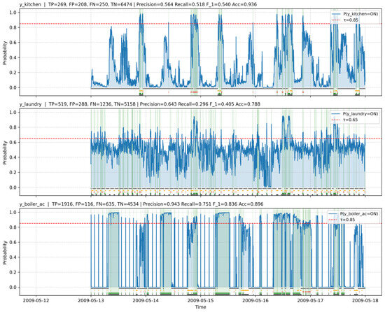
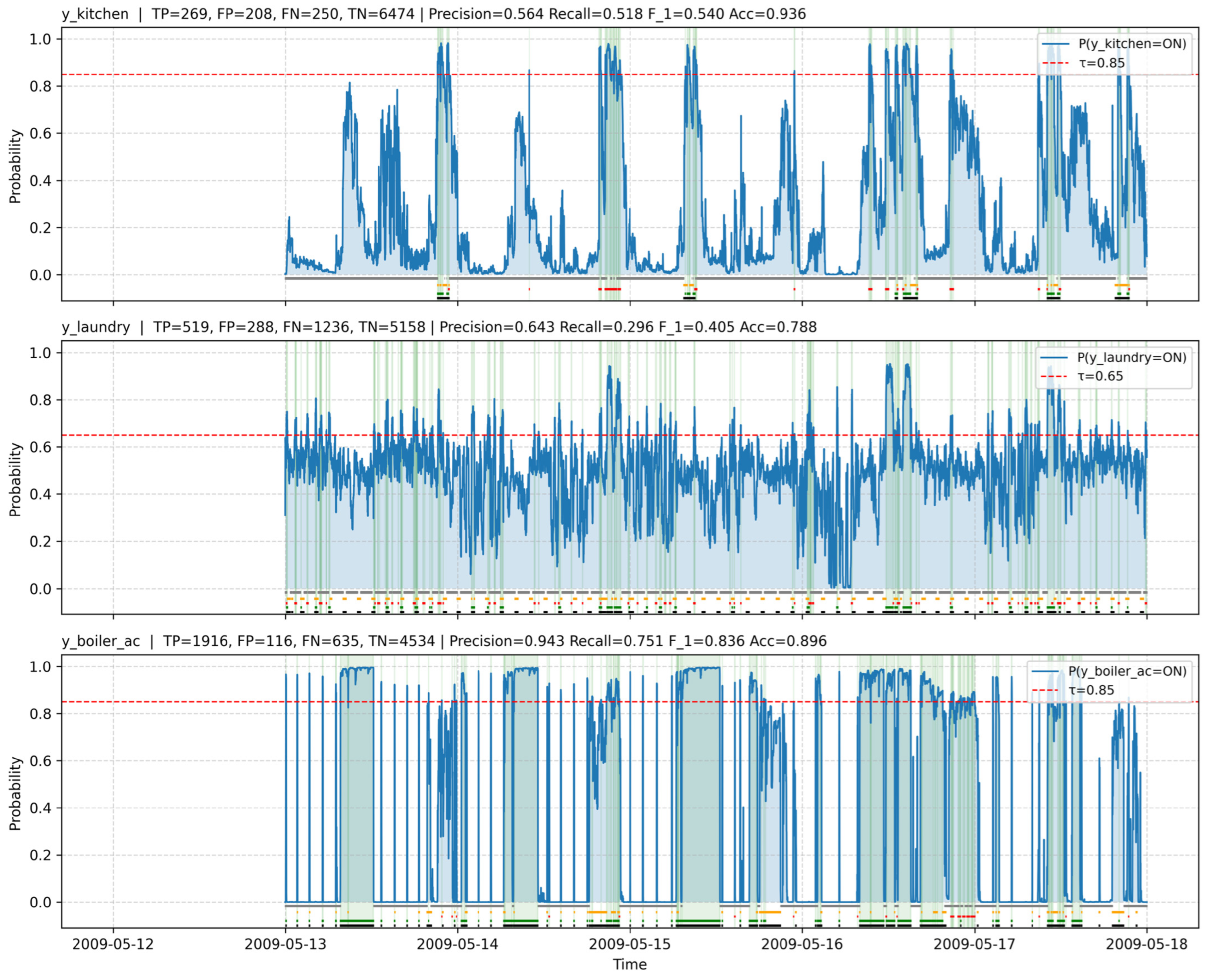
Finally, Step 9 performs a strict evaluation of model quality (Figure 3). Two groups of metrics are computed:
Figure 3.
Output of the HGB model for three load groups.
- Classical (sample-wise) metrics: precision (P), recall (R), , accuracy (ACC), and integral probabilistic measures—area under the precision–recall curve (AP) and area under the receiver operating characteristic curve (ROC-AUC). These metrics assess the model’s ability to assign the correct class at each minute of observation.
- Event-based metrics: a true positive event is counted if the start or end of a predicted “on” interval falls within a tolerance of relative to the true interval. Event-based precision (P), recall (R), and are computed, along with counts of missed events and false alarms. This evaluation aligns with operational requirements, where the correct detection of complete ON/OFF episodes is more important than minute-level labels.
In Figure 3, the dotted line indicates the threshold, and the horizontal lines below (green, yellow, red, and black) refer to the results as TP, FP, TN, and FN, respectively.
Overall, the proposed algorithm enables the automatic extraction of operating states of individual end-use devices from an aggregated electricity consumption signal using machine learning methods based exclusively on active power data. By combining hysteresis-based labeling with GAP feature engineering and probabilistic classification, followed by calibration and binarization-threshold optimization, high state-detection accuracy is achieved without direct metering of each load. As a result, the method provides a foundation for intelligent power supply system control in which load states can be assessed in near real time with a controllable balance between sensitivity and recognition reliability.
2.3. Evaluation Metrics
During model development, a set of dedicated metrics was used to demonstrate the correctness and adequacy of the binary classifier. In total, 11 metrics were employed, grouped into three categories: (1) sample-wise; (2) probabilistic; and (3) event-based.
Each metric serves a specific purpose. Sample-wise metrics, partially introduced in Section 2.2, quantify classification quality at each time step (each minute is treated as an individual sample). This group includes the standard metrics ACC, precision, recall, and .
The probabilistic-metric group includes ROC-AUC (area under the receiver operating characteristic curve) and AP (average precision). These measures do not assess the final binary decisions directly; instead, they evaluate the quality of the model output as a probability function .
ROC-AUC is the area under the ROC curve, which describes the relationship between the true positive rate (TPR) and the false positive rate (FPR). The closer ROC-AUC is to 1, the better the model separates classes irrespective of the chosen threshold.
To construct the ROC curve, the threshold is varied iteratively from 0 to 1 and, at each iteration, the following quantities are computed:
Thus, the ROC curve is the locus of points in the (FPR, TPR) plane obtained for all possible . ROC-AUC is then computed as:
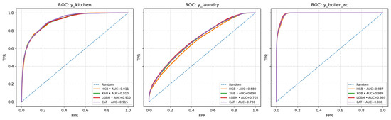
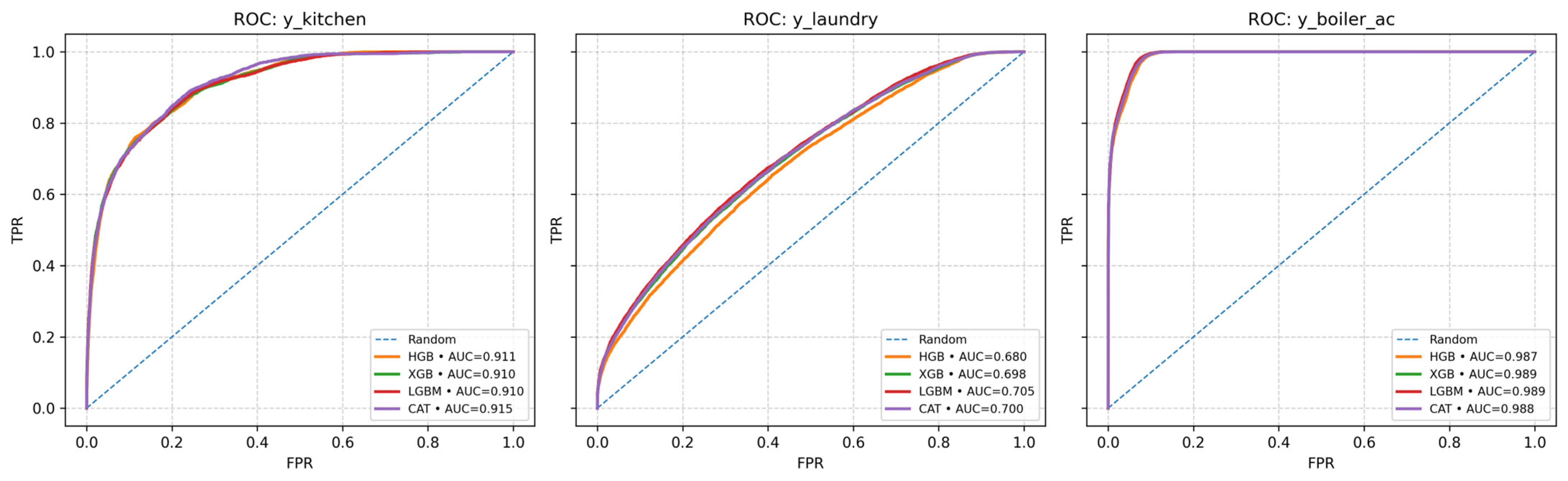
Therefore, ROC-AUC (Figure 4) is invariant with respect to the selected threshold and reflects the model’s ability to discriminate between device states.
Figure 4.
ROC curves for different models. The dash–dot line corresponds to a random classifier.
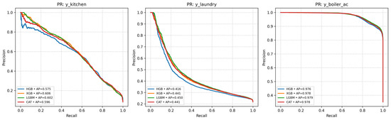
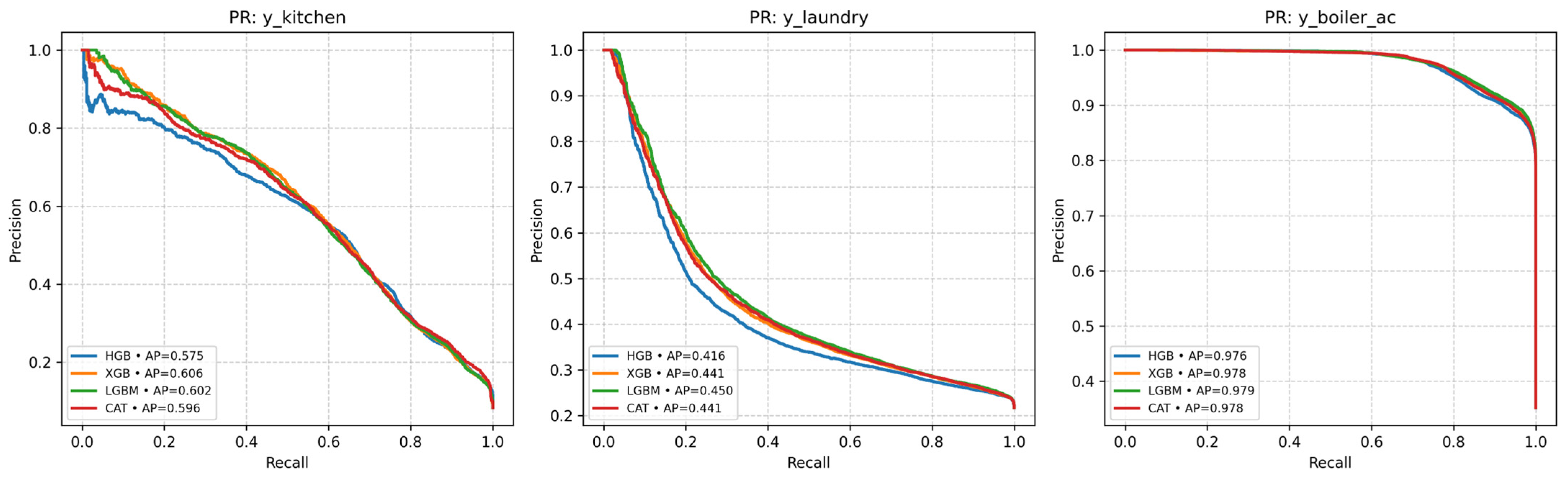
The AP metric corresponds to the area under the precision–recall (PR) curve and focuses on the model’s performance in predicting the positive class. PR curves were mentioned earlier; here, we provide the computation method and visualization in Figure 5. In general form, AP is defined as the integral:
Figure 5.
Precision–recall curves (AP) for different models.
Event-based metrics, unlike the previous two groups, evaluate model performance not at the level of individual time steps (i.e., treating each minute as a separate object and counting TP/FP/FN/TN), but at the level of switching intervals—on and off episodes of the end-use device. This metric group better reflects the requirement for stable operation and is closer to human perception of “events”.
The event-based group includes: Precisionevent, Recallevent, F1event. The base counts TP/FP/FN/TN are computed using the rule that an event is considered correctly detected if the start or end of the predicted “ON” interval falls within a tolerance of minutes relative to the ground-truth interval.
As an example, for the GAP-only model, both sets of metrics (sample-wise and event-based) were computed. The results are summarized in Table 1.
As shown in Table 1, the TP/FP/FN/TN counts become substantially smaller when moving from sample-wise to event-based evaluation. The metric values also decrease for loads that are weakly distinguishable. These results (Table 1 and the associated ROC/PR curves) were obtained using the primary chronological split with 336 training days followed by 21 validation days.
2.4. Sensitivity Analysis
2.4.1. Feature Selection Sensitivity
To assess the robustness of the proposed two-stage feature selection procedure (collinearity removal followed by permutation importance ranking), we conducted a sensitivity analysis along two dimensions. First, we varied the correlation threshold used to remove highly collinear predictors from the GAP-derived feature set, testing . Second, we evaluated whether the permutation importance ranking depends on the choice of the estimator by computing permutation importance using the baseline estimator (HGB) and the final selected model (LGBM). In all cases, the feature selection steps were fitted strictly on the training window (chronological split), while model quality was evaluated on the fixed chronological validation window, consistent with the main experiment.
Table 2 summarizes the results. When varying the correlation threshold, the number of retained features changed only slightly (14 features for |r| > 0.98 vs. 12 features for |r| > 0.95/0.90).
The resulting performance variations were limited: the largest absolute deviations across targets were and .
When switching the permutation importance estimator from HGB to LGBM (with |r|>0.98), AP remained effectively unchanged ( across targets), while event-based F1 changed modestly (). Overall, these results indicate that the feature selection stage is not brittle with respect to reasonable variations of the collinearity threshold and the choice of the permutation importance estimator.
Table 3 shows the results of calculating sensitivity to model selection when calculating permutation importance in the question of feature selection.
All feature selection steps were performed using training data only (chronological split); the reported metrics are computed on the fixed chronological validation window.
2.4.2. Sensitivity Analysis for the Post-Processing Window Length
To justify the post-processing window length W used in Step 8, we performed a sensitivity analysis of the causal moving average smoothing applied to calibrated probabilities. We evaluated minutes using the same strictly chronological split and the same calibration protocol described in Section 2.2.
For each W, the decision threshold was re-optimized on the validation window using the target-specific objective (with as defined in Section 2.2), and both sample-wise and event-based metrics were computed. In addition, we report the worst-case additional latency induced by causal smoothing as min.
Table 4 shows that increasing W consistently reduces the number of false-alarm events () but increases missed events (), i.e., a classical precision–recall trade-off. For example, when moving from to , decreases from 120 to 94 for the boiler/AC group, from 139 to 118 for the kitchen group, and from 310 to 272 for the laundry group, while increases accordingly.
Although yields the highest event-based F1 for some targets, we retain as the baseline because it provides a more conservative operating point with fewer spurious triggers (false alarms) while keeping the causal smoothing latency within 4 min at sampling, which is acceptable for the targeted DR feedback loop.
3. Results
3.1. Computational Performance
Training the baseline machine learning models yielded the following observations. Depending on the model, training and validation times differed, which directly affects the suitability of specific approaches for online deployment and for integration into demand-response control systems.
LGBM demonstrated the best performance in terms of both training and inference speed. This can be attributed to implementation characteristics: the histogram-based algorithm and efficient parallelization enable high throughput while maintaining classification quality. HistGradientBoosting, despite relying on a similar principle, is somewhat slower, which can be explained by implementation constraints in the scikit-learn Python library (version 1.4.2, Python version—3.11.6).
XGBoost provides stable performance and strong predictive quality; however, under comparable training settings, it is slower than LGBM, particularly on CPU. This is related to less aggressive optimizations in memory handling and parallel execution.
CatBoost, in contrast, is particularly effective when categorical features are present; nevertheless, its computational performance is the lowest among the models considered. This can be attributed to additional computational overhead for handling categorical variables, as well as a more complex, multi-stage optimization procedure.
Overall, based on the computational-performance analysis, the models can be ranked in descending order of speed as follows: LGBM → HGB → XGB → CAT.
More complex neural network models—specifically LSTM-based architectures reported in [25,26] and neural networks of various configurations described in [27,28]—are not suitable for implementation on low-power computing hardware in online mode. Recent NILM studies in IEEE Transactions on Industrial Informatics demonstrate that deep-learning approaches can reach high disaggregation accuracy, including CNN-based trajectory and multi-feature representations and efficient architectures with local feature extraction. However, these methods typically assume richer measurement modalities and/or substantially higher computational budgets compared with the GAP-only, edge-oriented setting considered in this paper. Therefore, we focus on lightweight gradient boosting baselines and explicitly quantify the accuracy–latency trade-offs under strict deployability constraints [29,30]. This limitation becomes a practical barrier to deploying the demand-response programs considered in this paper when load state monitoring is included as part of the control loop, even when using relatively lightweight machine learning approaches.
At the same time, it should be noted that recent edge-oriented neural approaches attempt to mitigate the above limitation via model-compression techniques, including pruning, quantization, and knowledge distillation. These methods reduce the memory footprint and inference cost of deep models, potentially enabling deployment on constrained hardware. However, they address a different design point compared with the present work: compressed neural networks still require a dedicated neural runtime, and their effective latency and energy consumption may remain hardware-dependent, while calibration and decision-thresholding for event-level objectives can introduce additional complexity. In contrast, the proposed pipeline is lightweight by construction and provides predictable computational requirements without specialized neural network stacks. For the binary state-detection task considered here, this design choice yields an efficient baseline suitable for online DR feedback; nevertheless, compressed neural models remain a promising extension for hybrid schemes, in which a lightweight detector triggers a selectively invoked neural module to resolve ambiguous events under strong load overlap.
3.2. Accuracy
In addition to computational performance, model accuracy (according to the metrics described above) was evaluated as a function of the number of days used for training/validation. This analysis supports deployment-oriented assessment, including indicative timelines for data acquisition, commissioning, and routine operation.
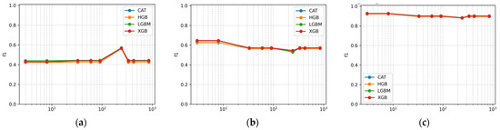
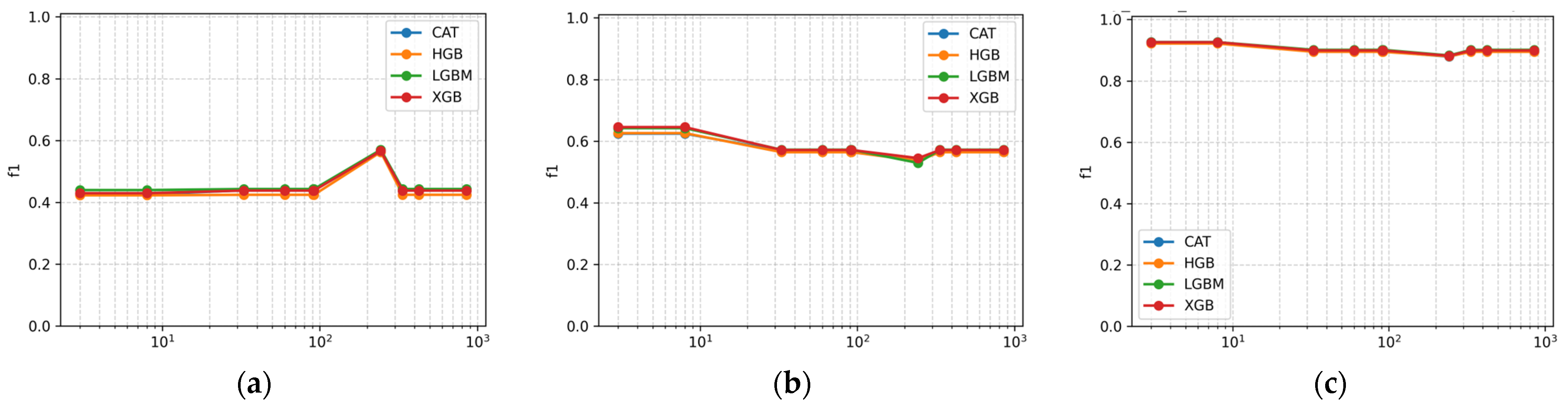
Figure 6 presents the score for each model as a function of the number of training days. Note that, for each training set size, the validation interval was selected using physically and logically justified durations: 3/5/7 days when the training set size was up to one year, and 30/60/90 days when the training set size was up to three years. This approach allows validation of the resulting model on time intervals that capture relevant operating periodicities of equipment, shift patterns, and both working and non-working days (including holidays).
Figure 6.
score as a function of training set size for different targets.
Based on Figure 6, it can be concluded that the dataset size does not affect model accuracy in any consistent manner. Figure 6 reports a sensitivity study where the training horizon is varied; the corresponding validation horizon is also varied to maintain a realistic evaluation period, while preserving the strictly chronological split defined in Section 2.2.
For load (b), represented as an aggregated load group associated with the kitchen, contrary to expectations, increasing the training set size had a negative impact on the final metrics.
For load (a), represented as an aggregated load group labeled “laundry”, a spike in model accuracy is observed, which may be interpreted as a data outlier without an interpretable physical meaning.
3.3. Cross-Seasonal Validation
Household load patterns are known to vary seasonally, especially for HVAC/boiler-related end-use consumption. To evaluate robustness under seasonal shifts, we performed an additional cross-seasonal experiment using strictly chronological, non-overlapping windows. In both cases, the baseline LGBM model was trained on a contiguous historical window, probability calibration (isotonic regression) was fitted only on a dedicated calibration sub-window taken from the end of the training period immediately preceding the validation window, and the final evaluation was conducted on a 21-day validation window from a different season (no information leakage).
We considered two representative season shifts: winter/spring→summer (validation 1 July 2007 to 21 July 2007) and summer/fall→winter (validation 10 January 2008 to 30 January 2008). Table 5 reports AP and event-based performance (±3 min tolerance) for the three targets at the baseline post-processing settings min and target-specific . For the boiler/AC group, performance remains high in the winter/spring→summer case (, , ) but degrades under the summer/fall→winter shift (, ), mainly due to an increase in false-alarm events () despite high recall (). For kitchen and laundry, event-based scores remain low in both season shifts ( for kitchen; for laundry), indicating that these weaker/overlapping load groups are intrinsically harder to identify from GAP-only features and are more sensitive to behavioral variability.
Table 5.
Cross-seasonal validation results for the baseline LGBM model.
3.4. Brief Error Analysis
While the score provides a compact summary, it does not explain the dominant failure modes of GAP-only state inference. Visual inspection of validation windows indicates three typical scenarios.
- Load overlap and correlated switching: false positives appear when a non-target device produces a power step similar in magnitude and duration to the target group, particularly during periods of high household activity (evening hours), where multiple appliances switch in close succession.
- Short and weak events: false negatives are more frequent for short-duration operating intervals and low-power patterns (notably for the kitchen and laundry groups), where the ON interval is comparable to the smoothing window W and can be suppressed by post-processing rules designed to remove spurious spikes.
- Boundary/transition artefacts: errors cluster near state transitions when the probability trajectory crosses the decision threshold slowly due to gradual ramps or mixed operation; this produces fragmented events (FP/FN pairs) which pointwise metrics penalize more strongly than event-based metrics with time tolerance.
These observations reinforce the design trade-off of Step 8: increasing W reduces spike-driven false alarms but may miss short events and increases detection latency. Consequently, we report event-based metrics alongside sample-wise measures and include sensitivity results to guide parameter selection under different DR cost asymmetries.
3.5. Application of the Algorithm to Demand Response
Based on the comparative analysis of several machine learning models, we conclude that, as a first approximation, they exhibit similar accuracy in the binary classification setting. Therefore, a rational model choice is to prioritize computational performance, as indicated by the runtime analysis [31].
Given the deployment requirements for a subsystem that monitors load response to demand-response control signals, LGBM was selected as the baseline model. This choice is motivated by the combination of predictive performance and computational efficiency identified in the conducted evaluation. This conclusion is consistent with findings from related applied domains, where LGBM demonstrates a comparable advantage under the “accuracy–speed” trade-off criterion [32,33].
4. Discussion
From a scalability perspective, the results of this study should be evaluated on a broader electricity consumption database. The present work reports results for only three load groups, which also differ in their operational characteristics (as described in Section 2). One direction for further improvement is to expand the pool of end-use devices (or load groups) to be identified within the aggregated consumption profile.
The proposed emphasis on computationally efficient models, rather than heavier and potentially more accurate approaches, may raise questions regarding the sufficiency of the resulting load-activation probability estimates. However, confirming the validity of these models under field conditions requires additional investigation, including the formulation and evaluation of a cost-sensitive error function, as performed in [34].
Importantly, moving from sample-wise metrics (ACC, Precision, Recall, F1) to event-based metrics leads to an expected decrease in scores and reveals the most vulnerable load classes—primarily low-power and short-duration loads. This finding supports the use of event-based evaluation specifically for NILM in demand response, because the operational value lies less in “minute-by-minute correctness” and more in the correct detection of ON/OFF episodes.
4.1. Areas for Future Research
In addition, a promising research direction is to integrate the proposed system architecture into a hierarchical two-level condition-monitoring framework for electromechanical equipment [35,36]. The current NILM implementation, operating at a low sampling rate, effectively addresses the first level: status identification. For preventing fault conditions, the second level is critical—technical condition diagnosis based on high-frequency electrical-parameter signals [37].
Within a two-level framework, NILM acts as an intelligent trigger to initiate computationally expensive diagnostic procedures, which involve deep spectral analysis of current signals required for defect detection in induction motor drives [38,39,40]. Consequently, continuous execution of such diagnostic computations on edge devices is inefficient or even infeasible [41]. An event-based model can substantially reduce computational and communication requirements, because the diagnostic algorithm is activated only when a stable operating regime of the motor is identified [42].
Active power, analyzed at the first level, can serve as an adaptive parameter for the second level, since the sensitivity of current-based diagnostic algorithms depends directly on the motor loading factor [43]. Information from the NILM module enables dynamic adjustment of diagnostic features, facilitating adaptive algorithms with high reliability across the full range of operating loads [37]. Taken together, these considerations justify the integration of demand-response control and technical diagnostics within a unified system.
This work demonstrates the practical feasibility of monitoring the states of individual end-use devices from an aggregated electricity consumption signal without installing additional measurement channels. The proposed algorithm combines hysteresis-based labeling, construction of a restricted set of GAP features, selection of informative predictors, and subsequent training of classical gradient boosting models. This approach yields operationally usable probabilistic estimates of the “ON/OFF” states even under partial metering coverage and in the presence of a noise component that approximates real-world networks.
4.2. Feature Importance
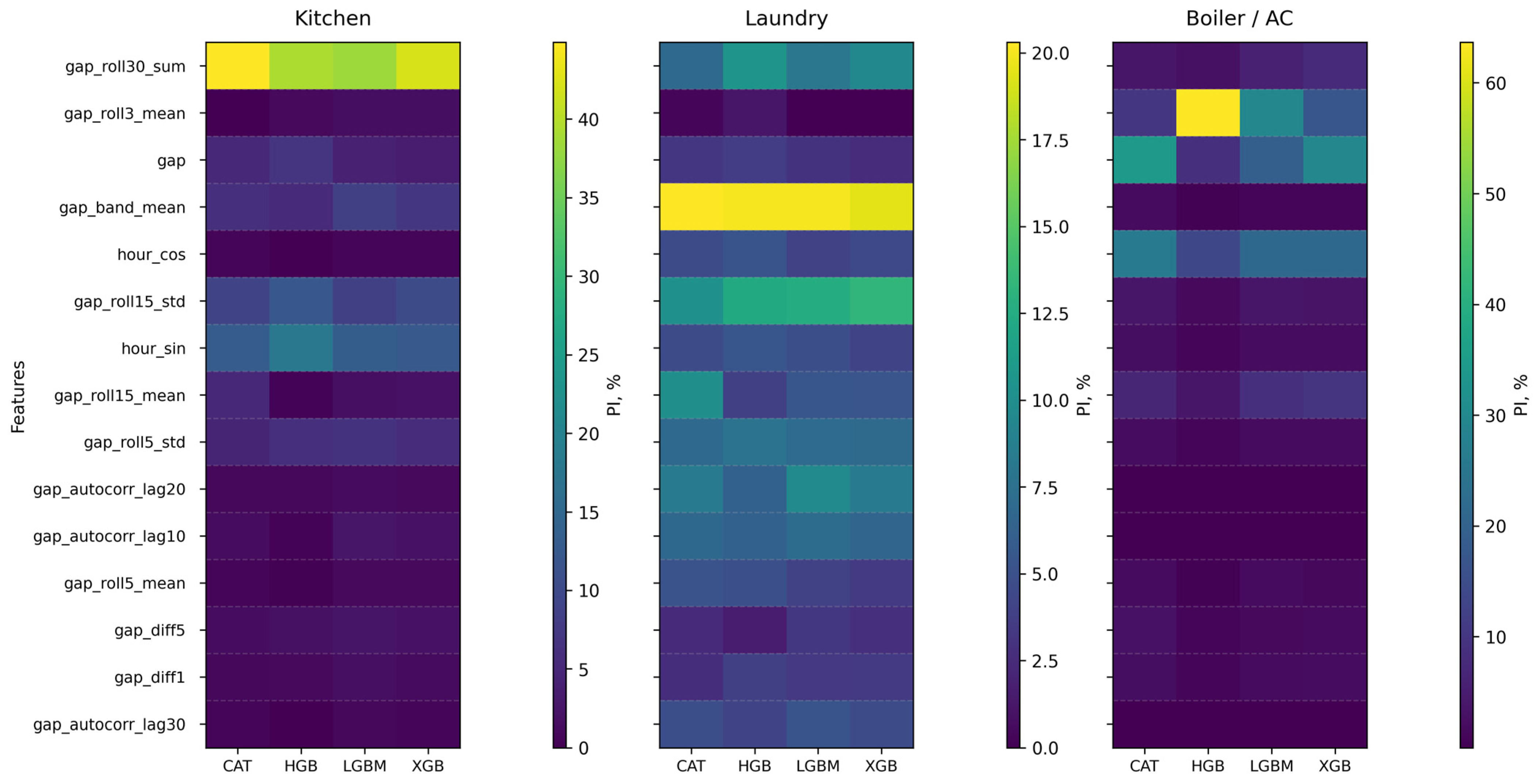
Feature importance was also assessed. Figure 7 shows a heatmap of the most informative features derived from the aggregated electricity consumption time series P(t). Each feature represents either local signal statistics within a moving window, signal derivatives (dynamics), or temporal periodicity. The features used are defined as follows:
Figure 7.
Importance of GAP features for each model and each load group.
- 1.
- gap—the raw aggregated signal value P(t) at the current time; a baseline informative feature representing the consumption level.
- 2.
- gap_roll3_mean—moving mean over a 3-min window; smooths high-frequency noise and captures short-term trends.
- 3.
- gap_roll5_std—moving standard deviation over a 5-min window; characterizes local variability and the presence of impulsive changes.
- 4.
- gap_roll15_mean—moving mean over a 15-min window; describes a more inertial load component and stable consumption regimes.
- 5.
- gap_roll15_std—moving standard deviation over a 15-min window; reflects medium-term instability/volatility of the signal on the order of a quarter-hour.
- 6.
- gap_roll30_sum—moving sum over a 30-min window; interpretable as integrated (accumulated) energy over a half-hour horizon and associated with the duration/intensity of activations.
- 7.
- gap_band_mean—a band-pass feature defined as the difference between two moving means of different lengths: It highlights variations on the scale of several minutes while suppressing slow drift and very fast noise.
- 8.
- gap_autocorr_lag20—local autocorrelation of P(t) at a 20-min lag, computed within a moving window (20 points in the implementation); describes pattern repetitiveness over a min horizon and is suitable for detecting quasi-periodic operating regimes.
- 9.
- hour_sin—sinusoidal cyclic encoding of the hour-of-day. Computes as follows: , where is the hour-of-day extracted from the timestamp; it provides a continuous representation of daily periodicity without an artificial discontinuity between 23:00 and 00:00.
- 10.
- hour_cos—cosine cyclic encoding of the hour-of-day. The pair ( jointly represents the phase of the daily cycle and allows the model to capture regular diurnal dependencies in device activation probability.
4.3. Cybersecurity Aspect
The proposed NILM-based feedback pipeline assumes a trustworthy metering and communication layer. Targeted adversarial manipulation of aggregate measurements (e.g., false-data injection or load-masking attacks) may distort the inferred device states and is not explicitly addressed by the present work. Developing dedicated detection/mitigation mechanisms for such cyber–physical threats is beyond the scope of this paper; interested readers are referred to recent work on smart-grid attacks and defenses [44,45].
4.4. Transferability to Higher Resolution Measurements
The experimental validation in this work is intentionally restricted to a public residential dataset to ensure reproducibility and to match common DR feedback settings in which only low-rate smart-meter GAP streams are available. Therefore, the reported numerical results should be interpreted as a benchmark under a low-information regime rather than as universal performance bounds.
From an identifiability perspective, increasing the sampling rate is expected to improve detection of short-duration and weak loads by preserving transient switch-on/off edges, reducing temporal aliasing, and enabling more informative causal features. In practice, higher resolution can reduce missed events for brief operating intervals and may allow smaller smoothing windows W while maintaining robustness, thereby improving event-based metrics and decreasing latency. At the same time, higher resolution does not eliminate ambiguity under multi-device overlap; in such cases, additional modalities may still be required.
Transfer to industrial and commercial settings is non-trivial because load composition, schedules, and process-driven variability differ from households. The proposed pipeline remains applicable as a generic, lightweight baseline, but deployment in I&C power supply systems would require target-specific re-tuning of , W, and adaptive thresholds, and validation on representative non-residential datasets. Extending the feature vector with process- and power-quality-related predictors appears particularly promising for I&C scenarios.
5. Conclusions
Comparison of multiple machine learning models indicates that, given similar sample-wise and event-based metrics, computational performance becomes the decisive factor for industrial use. On the Household Power Consumption dataset (1-min resolution) using a strictly chronological split (336 training days followed by 21 validation days), the proposed GAP-only pipeline with LGBM achieves high threshold-free performance and competitive event detection quality across the three load groups. In terms of average precision (AP), the best-performing configuration reaches approximately 0.98 for the boiler/AC group, about 0.60 for the kitchen group, and about 0.44 for the laundry group. Under the event-based evaluation with a ±3-minu tolerance, the corresponding event-based F1 scores are approximately 0.77 (boiler/AC), 0.23 (kitchen), and 0.28 (laundry). These values summarize the main operating region of the method and highlight that the strongest performance is achieved for loads with clearer aggregate signatures, while the weakest/imbalanced group (laundry) remains the most challenging case. Based on the results, LGBM is the most suitable baseline model, providing the shortest training and validation times while maintaining the required accuracy. HistGradientBoosting, XGBoost, and CatBoost also demonstrate satisfactory performance; however, their use under the considered constraints is less justified.
The obtained results can be viewed as a first step toward deploying sensorless monitoring within a demand-response control loop: the algorithm can be deployed on edge devices without requiring a dedicated compute cluster and without imposing stringent bandwidth requirements on communication channels.
Further work should include: (a) expanding the set and number of monitored loads, including weakly distinguishable loads and devices with highly variable consumption patterns; (b) evaluating robustness on datasets with different consumption profiles (shift schedules, seasonality, process shutdowns); (c) investigating hybrid schemes in which classical gradient boosting models serve as a lightweight online detector, while heavier neural network models are used to improve event-based metrics and resolve ambiguous cases; (d) assessing robustness to potential drift in feature importance driven by consumption trends. In addition, it appears promising to augment the training feature vectors with process-related features, as in [46], and with features specific to industrial power supply systems, for example, a power-quality feature vector.
Author Contributions
Conceptualization, Y.Z. and P.S.; methodology, P.S.; software, P.S.; validation, P.S. and D.R.; formal analysis, D.R.; investigation, P.S. and D.R.; data curation, D.R.; writing—original draft preparation, P.S.; writing—review and editing, Y.Z.; visualization, P.S.; supervision, Y.Z.; project administration, Y.Z.; funding acquisition, Y.Z. All authors have read and agreed to the published version of the manuscript.
Funding
This research has no funding.
Data Availability Statement
The “Individual Household Electric Power Consumption” dataset analyzed in this study is publicly available as described in Ref. [22]. The code and processed data required to reproduce the results are available from the corresponding author upon reasonable request.
Acknowledgments
ChatGPT-5.2 was used exclusively for language editing (grammar correction) in limited sections of the manuscript. The authors reviewed and validated all revisions to confirm that the meaning and technical content were preserved. The authors assume full responsibility for the final manuscript and its contents.
Conflicts of Interest
The authors declare no conflicts of interest.
Abbreviations
The following abbreviations are used in this manuscript:
| DR | Demand response |
| NILM | Non-intrusive load monitoring |
| GAP | Global active power |
| SCADA | Supervisory Control and Data Acquisition |
| ACC | Accuracy |
| HGB | Histogram-based Gradient Boosting |
| XGB | Extreme Gradient Boosting |
| LGBM | Light Gradient Boosting Machine |
| CAT | Categorical Gradient Boost algorithm |
| ML | Machine learning |
| MAD | Median absolute deviation |
| AP | Average precision |
| LSTM | Long Short-Term Memory |
| TP | True positive |
| FP | False positive |
| TN | True negative |
| FN | False negative |
| ROC | Receiver operating characteristic |
| AUC | Area under ROC curve |
References
- Zhukovsky, Y.L.; Suslikov, P.K. Identification and classification of electrical loads in mining enterprises based on signal decomposition methods. J. Min. Inst. 2025, 275, 5–17. [Google Scholar]
- Rodríguez-Gómez, F.; del Campo-Ávila, J.; Mora-López, L. A novel clustering based method for characterizing household electricity consumption profiles. Eng. Appl. Artif. Intell. 2024, 129, 107653. [Google Scholar] [CrossRef] [Scilit]
- Stotzer, M.; Gronstedt, P.; Styczynski, Z.; Buchholz, B.M. Demand side integration—A potential analysis for the German power system. In Proceedings of the 2012 IEEE Power and Energy Society General Meeting, San Diego, CA, USA, 22–26 July 2012; IEEE: Piscataway, NJ, USA, 2012; pp. 1–8. [Google Scholar]
- Belskiy, A.A.; Emelyanov, E.A. Evaluation of indicators of autonomous electrical system with diesel and wind power plants. Gorn. Zhurnal 2025, 9, 37–44. [Google Scholar] [CrossRef] [Scilit]
- Serikov, V.A.; Sychev, Y.A.; Kostin, V.N.; Samet, H. Influence of active inductor–capacitor filter on amplitude–frequency characteristic of resonant mode power supply in industry. Min. Informational Anal. Bull. 2025, 7, 170–183. [Google Scholar] [CrossRef] [Scilit]
- Islam Bhuian, M.T.; Islam, M.S.; Uddin, M.F. Shared Encoder with Attention for Non-Intrusive Appliance Load Monitoring. In Proceedings of the 2023 10th IEEE International Conference on Power Systems (ICPS), Cox’s Bazar, Bangladesh, 13–15 December 2023; IEEE: Piscataway, NJ, USA, 2023; pp. 1–6. [Google Scholar]
- Jiao, R.; Li, C.; Xun, G.; Zhang, T.; Gupta, B.B.; Yan, G. A Context-Aware Multi-Event Identification Method for Nonintrusive Load Monitoring. IEEE Trans. Consum. Electron. 2023, 69, 194–204. [Google Scholar] [CrossRef] [Scilit]
- Voropai, N.; Ukolova, E.; Gerasimov, D.; Suslov, K.; Lombardi, P.; Komarnicki, P. A Study on Cost-Effectiveness of Energy Supply Based on the Energy Hub Concept. In Proceedings of the 2019 IEEE PES Innovative Smart Grid Technologies Europe (ISGT-Europe), Bucharest, Romania, 29 September–2 October 2019; IEEE: Piscataway, NJ, USA, 2019; pp. 1–4. [Google Scholar]
- Cruz-Rangel, D.; Ocampo-Martinez, C.; Diaz-Rozo, J. Online non-intrusive load monitoring: A review. Energy Nexus 2025, 17, 100348. [Google Scholar] [CrossRef] [Scilit]
- Kaselimi, M.; Protopapadakis, E.; Voulodimos, A.; Doulamis, N.; Doulamis, A. Towards Trustworthy Energy Disaggregation: A Review of Challenges, Methods, and Perspectives for Non-Intrusive Load Monitoring. Sensors 2022, 22, 5872. [Google Scholar] [CrossRef] [Scilit]
- Fathollahi, A. Machine Learning and Artificial Intelligence Techniques in Smart Grids Stability Analysis: A Review. Energies 2025, 18, 3431. [Google Scholar] [CrossRef] [Scilit]
- Dash, S.; Sahoo, N.C. Attention-Based Multitask Probabilistic Network for Nonintrusive Appliance Load Monitoring. IEEE Trans. Instrum. Meas. 2023, 72, 1–12. [Google Scholar] [CrossRef] [Scilit]
- Dash, S.; Sahoo, N.C. A Multi-Task Deep Learning Approach for Non-Intrusive Load Monitoring of Multiple Appliances. IEEE Trans. Smart Grid 2024, 15, 3337–3340. [Google Scholar] [CrossRef] [Scilit]
- Adewole, K.S.; Torra, V. Energy disaggregation risk resilience through microaggregation and discrete Fourier transform. Inf. Sci. 2024, 662, 120211. [Google Scholar] [CrossRef] [Scilit]
- Fedorova, E.; Morgunov, V.; Lobko, K.; Pupysheva, E. Review: Axial Motion of Material in Rotary Kilns. Eng 2025, 6, 106. [Google Scholar] [CrossRef] [Scilit]
- Belsky, A.A.; Ngyen, V.T.; Sheikhi, M.H.; Starshaia, V.V. Analysis of specifications of bifacial photovoltaic panels. Renew. Sustain. Energy Rev. 2025, 224, 116092. [Google Scholar] [CrossRef] [Scilit]
- Zhang, X.; Zhou, J.; Lu, C.; Song, L.; Meng, F.; Wang, X. Non-Intrusive Load Monitoring Based on Dimensionality Reduction and Adapted Spatial Clustering. Energies 2024, 17, 4303. [Google Scholar] [CrossRef] [Scilit]
- Asres, M.W.; Ardito, L.; Patti, E. Computational Cost Analysis and Data-Driven Predictive Modeling of Cloud-Based Online-NILM Algorithm. IEEE Trans. Cloud Comput. 2022, 10, 2409–2423. [Google Scholar] [CrossRef] [Scilit]
- Nos, O.V.; Pudkova, T.V.; Nos, N.I. The sliding-mode observer for PMSM field-oriented sensorless control with adaptive filter and PLL. Sci. Tech. J. Inf. Technol. Mech. Opt. 2024, 24, 415–423. [Google Scholar] [CrossRef] [Scilit]
- Shklyarskiy, Y.; Andreeva, I.; Sutikno, T.; Jopri, M.H. Energy management in hybrid complexes based on wind generation and hydrogen storage. Bull. Electr. Eng. Inform. 2024, 13, 1483–1494. [Google Scholar] [CrossRef] [Scilit]
- Hamani, K.; Kuchar, M.; Kubatko, M.; Kirschner, S. Advancements in Induction Motor Fault Diagnosis and Condition Monitoring: A Comprehensive Review. Sensors 2025, 25, 5942. [Google Scholar] [CrossRef] [Scilit]
- Hebrail, G.; Berard, A. Individual Household Electric Power Consumption [Dataset]. UCI Mach. Learn. Repos. 2006. [CrossRef]
- Klyuev, R.; Bosikov, I.; Gavrina, O.; Madaeva, M.; Sokolov, A. Improving the energy efficiency of technological equipment at mining enterprises. In International Scientific Conference Energy Management of Municipal Facilities and Sustainable Energy Technologies EMMFT 2019; Advances in Intelligent Systems and Computing; Springer: Berlin/Heidelberg, Germany, 2021; Volume 1258, pp. 262–271. [Google Scholar] [CrossRef] [Scilit]
- Bulatov, Y.; Kryukov, A.; Kizhin, V.; Suslov, K.; Iliev, I.; Beloev, H.; Beloev, I. Modeling an Energy Router with an Energy Storage Device for Connecting Electric Vehicle Charging Stations and Sustainable Development of Power Supply Systems. Sustainability 2025, 17, 11041. [Google Scholar] [CrossRef] [Scilit]
- Azad, M.I.; Rajabi, R.; Estebsari, A. Non-Intrusive Load Monitoring (NILM) using Deep Neural Networks: A Review. In 2023 IEEE International Conference on Environment and Electrical Engineering and 2023 IEEE Industrial and Commercial Power Systems Europe (EEEIC/I&CPS Europe); IEEE: Piscataway, NJ, USA, 2023; pp. 1–6. [Google Scholar]
- Holmegaard, E.; Baun Kjaergaard, M. NILM in an Industrial Setting: A Load Characterization and Algorithm Evaluation. In Proceedings of the 2016 IEEE International Conference on Smart Computing (SMARTCOMP), St. Louis, MI, USA, 18–20 May 2016; IEEE: Piscataway, NJ, USA, 2016; pp. 1–8. [Google Scholar]
- Liu, G.; Liang, G.; Zhao, H.; Zhao, J.; Liu, J.; Wu, Z. A Temporal Convolutional Neural Network with Attention Mechanism for Industrial Non-Intrusive Load Monitoring. In Proceedings of the 2021 IEEE 5th Conference on Energy Internet and Energy System Integration (EI2), Taiyuan, China, 22–24 October 2021; IEEE: Piscataway, NJ, USA, 2021; pp. 3279–3284. [Google Scholar]
- Akbar, M.K.; Amayri, M.; Bouguila, N.; Wurtz, F.; Delinchant, B. Assessing the Effectiveness of Supervised and Semi-supervised NILM Approaches in an Industrial Context. In Proceedings of the 2023 6th International Conference on Computational Intelligence and Intelligent Systems, Tokyo, Japan, 25–27 November 2023; ACM: New York, NY, USA, 2023; pp. 7–13. [Google Scholar]
- Yang, L.; Li, X.; Sun, M.; Sun, C. Hybrid Policy-Based Reinforcement Learning of Adaptive Energy Management for the Energy Transmission-Constrained Island Group. IEEE Trans. Ind. Inform. 2023, 19, 10751–10762. [Google Scholar] [CrossRef] [Scilit]
- Zhang, N.; Yan, J.; Hu, C.; Sun, Q.; Yang, L.; Gao, D.W.; Guerrero, J.M.; Li, Y. Price-Matching-Based Regional Energy Market With Hierarchical Reinforcement Learning Algorithm. IEEE Trans. Ind. Inform. 2024, 20, 11103–11114. [Google Scholar] [CrossRef] [Scilit]
- Alwaz, N.; Bashir, M.M.; Rehman, A.U.; Ullah, I.; Galea, M. Sustainable Optimization of Residential Electricity Consumption Using Predictive Modeling and Non-Intrusive Load Monitoring. Sustainability 2025, 17, 11193. [Google Scholar] [CrossRef] [Scilit]
- Boldini, D.; Grisoni, F.; Kuhn, D.; Friedrich, L.; Sieber, S.A. Practical guidelines for the use of gradient boosting for molecular property prediction. J. Cheminform. 2023, 15, 73. [Google Scholar] [CrossRef] [Scilit] [PubMed]
- Ahn, J.M.; Kim, J.; Kim, K. Ensemble Machine Learning of Gradient Boosting (XGBoost, LightGBM, CatBoost) and Attention-Based CNN-LSTM for Harmful Algal Blooms Forecasting. Toxins 2023, 15, 608. [Google Scholar] [CrossRef] [Scilit] [PubMed]
- Ghyasuddin Hashmi, S.; Balaji, V.; Ahamed Ayoobkhan, M.U.; Shabbir Alam, M.; Anilkuamr, R.; Nishant, N.; Prasad Patra, J.; Rajaram, A. Machine Learning-Based Renewable Energy Systems Fault Mitigation and Economic Assessment. Electr. Power Compon. Syst. 2024, 1–24. [Google Scholar] [CrossRef] [Scilit]
- Saleem, M.H.; Taha, M.; Rehmani, M.A.A.; Tito, S.R.; Soltic, S.; Nieuwoudt, P.; Pandey, N.; Ahmed, M.D. A comprehensive review of machine learning and deep learning models for non-intrusive load monitoring: Performance, analyses, practical insights, and emerging trends. Appl. Intell. 2025, 55, 1020. [Google Scholar] [CrossRef] [Scilit]
- Nazarychev, A.; Iliev, I.; Manukian, D.; Beloev, H.; Suslov, K.; Beloev, I. Review of Operating Conditions, Diagnostic Methods, and Technical Condition Assessment to Improve Reliability and Develop a Maintenance Strategy for Electrical Equipment. Energies 2025, 18, 5832. [Google Scholar] [CrossRef] [Scilit]
- Tanoni, G.; Principi, E.; Squartini, S. Non-Intrusive Load Monitoring in industrial settings: A systematic review. Renew. Sustain. Energy Rev. 2024, 202, 114703. [Google Scholar] [CrossRef] [Scilit]
- Gultekin, M.A.; Bazzi, A. Review of Fault Detection and Diagnosis Techniques for AC Motor Drives. Energies 2023, 16, 5602. [Google Scholar] [CrossRef] [Scilit]
- Koteleva, N.; Korolev, N.; Kovalchuk, M. Industrial Metaverse and Technical Diagnosis of Electric Drive Systems. Appl. Sci. 2025, 15, 12699. [Google Scholar] [CrossRef] [Scilit]
- Skamyin, A.; Shklyarskiy, Y.; Lobko, K.; Dobush, V.; Sutikno, T.; Hatta Jopri, M. Impedance analysis of squirrel-cage induction motor at high harmonics condition. Indones. J. Electr. Eng. Comput. Sci. 2024, 33, 31. [Google Scholar] [CrossRef] [Scilit]
- Zhao, S.; Li, S.; Gao, P.; Ge, S.; Zhang, Z.; Shu, L. Data Model Compression Method Based on Iterative Pruning and Distillation for Edge Non-Intrusive Load Monitoring. J. Electr. Eng. Technol. 2025, 20, 3709–3722. [Google Scholar] [CrossRef] [Scilit]
- Melnikova, O.; Nazarychev, A.; Iliev, I.; Beloev, I.; Suslov, K. Diagnostic statistical characteristics of dielectric strength of power transformer oil insulation. Energy 2025, 340, 139169. [Google Scholar] [CrossRef] [Scilit]
- Qu, Y.; Wang, X.; Zhang, X.; Huang, S. An Adaptive Method for Multifault Diagnosis of Induction Motor Under Sharp Changing Speed and Load Condition. IEEE Trans. Ind. Inform. 2024, 20, 3275–3284. [Google Scholar] [CrossRef] [Scilit]
- Naderi, E.; Asrari, A. Cybersecurity Challenges in Power-to-X Integration. In Power-to-X in Regional Energy Systems; CRC Press: Boca Raton, FL, USA, 2025; pp. 284–298. [Google Scholar]
- Naderi, E. Securing the future: Integrating quantum computing and digital twin technologies into modern power & transportation systems for resilient smart cities against false data injection cyberattacks. Int. J. Crit. Infrastruct. Prot. 2025, 51, 100807. [Google Scholar] [CrossRef] [Scilit]
- Ilyushin, P.; Gaisin, B.; Shahmaev, I.; Suslov, K. An Algorithm for Identifying the Possibilities of Cascading Failure Processes and Their Development Trajectories in Electric Power Systems. Algorithms 2025, 18, 183. [Google Scholar] [CrossRef] [Scilit]

Disclaimer/Publisher’s Note: The statements, opinions and data contained in all publications are solely those of the individual author(s) and contributor(s) and not of MDPI and/or the editor(s). MDPI and/or the editor(s) disclaim responsibility for any injury to people or property resulting from any ideas, methods, instructions or products referred to in the content. |
© 2026 by the authors. Licensee MDPI, Basel, Switzerland. This article is an open access article distributed under the terms and conditions of the Creative Commons Attribution (CC BY) license.