The Influence of a Blade Leading-Edge Configuration with a Variable Lean and Inverse Arrow Shape Modification in an Annular Turbine Cascade on the Pressure Loss Coefficient ^†

Abstract

This publication presents results of a numerical study of a controlled flow nozzle blade with a modification added at the leading edge of an annular cascade. The presented three-dimensional shape is compared with one having a constant lean at the leading edge, which is currently used in power plants. The study compares the annular row loss coefficient for a relatively large blade length and for a blade length reduced by half. Calculations are performed for compressible and incompressible flows. Additionally, the blade rows are investigated with different boundary conditions at the inlet and outlet, divided into several groups, in order to evaluate their effectiveness at different secondary-flow intensities. In numerical simulations, a variable velocity distribution, total temperature, and total pressure are set at the inlet, and a mass flow rate or variable static pressure is set at the outlet. For the developed variants, a loss coefficient is calculated, and a comparison is made between the two proposed bladed rows: the first with a straight-line trailing edge and a constant circumferential lean at the leading edge, and the second with a variable lean in the circumferential direction and a reverse sweep at the leading edge.

1. Introduction

In conventional turbine cascades, the interblade channel is bounded by four surfaces: a profile surface on the back of the blade (SS—suction side), a concave profile surface on the adjacent blade (PS—pressure side), an outer limiting surface (shroud), and an inner limiting surface (hub). The viscous working-fluid flow surrounds the blade, forming a boundary layer along the profiles. Its thickness does not exceed 1–3 mm, but internal friction mainly occurs in the boundary layer. In the region sufficiently distant from the channel contours, the flow can, in some cases, be considered two-dimensional and inviscid; that is, the flow consists of a boundary layer and a core. A significant portion of the kinetic energy loss is concentrated in the boundary layer. The energy losses resulting from the interaction of the flow with the blade are called profile losses $\xi$_pr, and the losses caused by the interaction of the flow with the side walls of the channel and the blade edges are called endwall losses $\xi$_end. The present report investigates the total loss coefficient $\xi$ in a stationary blade row. It is the sum of the profile losses $\xi$_pr and the endwall losses $\xi$_end and is determined by numerical calculations or by experiments.

According to a study by GE [1,2], the profile and endwall losses in the nozzle and rotating rows, as well as the losses due to flow leakage through the gaps, account for approximately 90% of the total losses in the turbine stage. This means that in order to increase efficiency, measures must be taken to reduce profile and endwall losses. According to information from the same source, 15% of these losses are due to secondary flows and vortex formation at the boundary walls at the root and periphery in the stationary cascade. This means that any efforts undertaken during the design process to reduce these effects are justified and can lead to an increase in the turbine-stage efficiency. The internal efficiency nowadays for a single high-pressure steam turbine stage is around η_i ≈ 88–91%.

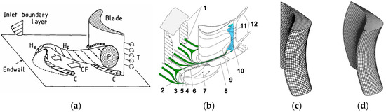
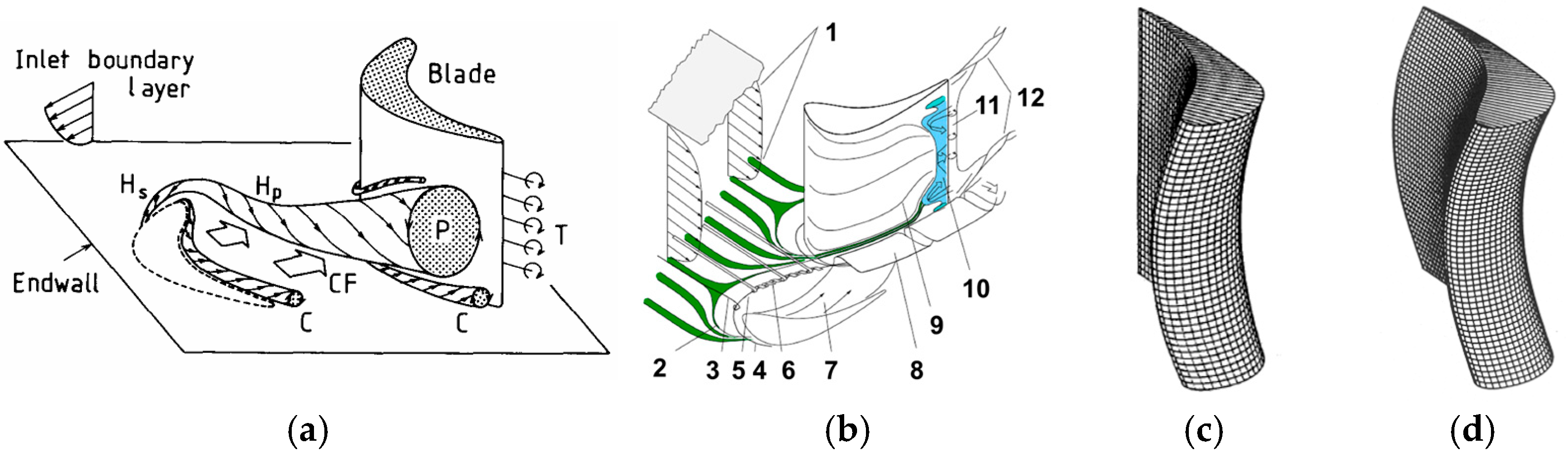
With short blades that strongly rotate the flow (ℓ/b = 4.45), a double vortex is formed in the channel. In this area, local losses reach 60–80% of the total flow energy losses. The shorter the blades, the larger the portion of the main flow occupied by the three-dimensional effects of the root and periphery. At a certain ratio (ℓ/b =ℓ_kr), the interaction of the two vortices from the end zones begins, which leads to a sharp increase in losses in the middle section of the channel (Figure 1a).

Figure 1. Formation of the secondary flows in an interblade channel in a cascade with cylindrical blades (a) [3], (b) [4], nozzle-type Control Flow Nozzle CFN (c) and Compound Lean Nozzle CLN (d) reprinted with permission from Ref. [5].

The secondary flows and the pair of vortices rotating in opposite directions consume part of the flow energy, increase the entropy of the fluid, and are associated with a decrease in the flow kinetic energy. They depend on numerous geometric and thermogas-dynamic parameters described in the specialized literature.

Figure 1a presents a model of vortex structures near the channel wall of a stationary cascade, proposed by Kawai [3]. Abbreviations are as follows: H_s—suction-side leg of horseshoe vortex; H_p—pressure-side leg of horseshoe vortex; C—vortices at corner between blade and endwall; CF—endwall crossflow; T—trailing vortex; P—passage vortex. The boundary layer at the inlet of the cascade interacts with the blade leading edges to generate the horseshoe vortices. The interblade pressure gradient drives the CF. The vortex H_p entrains the CF to create the passage vortex, P. Further towards the exit, the passage vortex, P, begins to grow as the pressure decreases. The C vortices are generated in the corners between the blades and the boundary wall, and the T vortices are observed after the trailing edge.

Figure 1b shows the secondary-flow generation according to another model proposed by Vogt [4]. The abbreviations are as follows: 1—velocity distribution at inlet; 2—inlet boundary layer separation; 3—horseshoe vortex core at inlet; 4—suction-side horseshoe vortex; 5—pressure-side horseshoe vortex; 6—inlet boundary layer rolling up; 7—passage crossflow; 8—passage vortex; 9—boundary layer movement on blade suction side; 10—separation with backflow; 11—wake eddies; 12—trailing-edge vortices. The Vogt and Zippel model is more detailed than Kawai’s, but they are essentially the same and represent the complex processes of energy transformation in the interblade channels of a modern turbine cascade.

In improving the flow path of a modern turbine, one way to reduce the intensity of secondary flows is by changing the three-dimensional shape of the turbine blades. In practice, blades of various shapes are used: arrow-shaped and lean-shaped. Some of the major companies produce the following blades: Siemens—3DV, 3DS [2]; GE—Controlled vortex, Advanced vortex [1]; Alstom—CFN, Controlled Flow 2-type (CF2) [6]; and many others. Three-dimensional blades with a variable lean at the leading edge (Control Flow Nozzle—CFN; Figure 1c) appeared in the nineties of the last century and were applied in the modernization of the 660 MW steam turbine unit, carried out by Alstom. The shape of the nozzle blade is obtained by rotating the profile at the midsection about a line passing through the straight trailing edge. This blade is applied in impulse-type turbine stages. Tests conducted in an experimental turbine show an increase in isentropic efficiency of 1.2%. This is also confirmed by computational fluid dynamics (CFD) modeling. New developments (CF2) proposed by Haller show that this blade design can be modified and used in reaction-type steam turbines and improve performance. The three-dimensional blade Compound Lean Nozzle (CLN) (Figure 1d) was created in the sixties by a team of scientists led by Prof. Deich from the Moscow Power Engineering Institute [6]. Its shape is obtained by moving the profile from the mid-cross-section in a circumferential direction. This leads to a circumferential variable lean of both the leading edge and the trailing edge. The CLN modification was tested in a two-stage experimental turbine at the Alstom laboratory. The data show that the efficiency of the stage with a CLN blade increases by about 0.5% compared to a turbine stage with a standard shape.

2. Geometrical Data on Blade Cascade

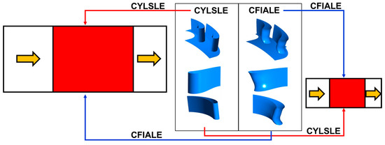
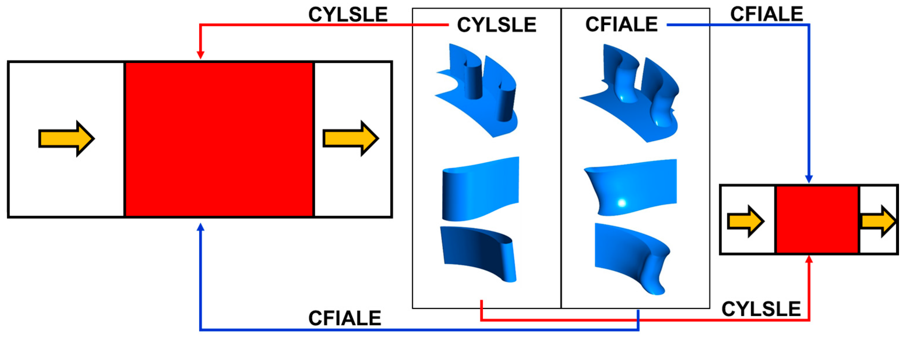
In this study, two models of cascades with turbine blade heights of 150 mm and 64 mm were developed. The profiles for both variants are the same but scaled. For clarity, the dimensions and details of the compared cascades are presented in Table 1. The first variant is a straight blade with a constant lean in the circumferential direction (CYL LEAN STRAIGHT LE, with the abbreviation CYLSLE). In the second variant, the leading edge of the blade has a constant inverse lean in the axial direction and a variable lean in the circumferential direction (CFN INVERSE ARROW LE, with the abbreviation CFIALE). These three-dimensional forms are shown in Figure 2. Unlike the Alstom CFN blade described above (Figure 1c), in this project a blade with a leading edge that is leaned in the axial direction opposite to the direction of fluid movement has been developed. In addition, the leading edge has a variable lean in the circumferential direction in the lower quarter of the blade’s length. From the middle section to the periphery, the blade has a straight shape. The trailing edge is straight. The abbreviation BC before the test number means boundary conditions. The first test group, simulation BC Test 1, is modeled with air as the working fluid and with long blades; the second group, BC Tests 2.1, 2.2, and 2.3, is modeled with superheated steam and short blades.

Table 1. Description of the main geometrical dimensions of the compared blade cascades.

Cascade Description	Long Blade BC Test 1	Short Blade BC Test 2.1, 2.2, 2.3
Length ℓ, mm	150	64
Row axial width B, mm	190	80
Chord c, mm	334	142
Stagger angle, deg	55.8°	55.8°
Inlet metal angle, deg	11–14°	11–14°
Outlet metal angle, deg	−78°	−78°
Pitch at hub, mm	200	85
Pitch at shroud, mm	230	98
LE axial lean, deg	74	74

Figure 2. Work plane scheme with 3D blades and meridional plane view. Arrows show flow direction.

In this work, annular cascades are modeled to account for the influence of the difference in pitch size at the root and at the periphery between the blades. This difference affects the secondary-flow intensity in these endwall zones. The small root pitch leads to increased velocity and bending of the flow towards the periphery, where the cross-section increases. This distortion of the streamlines leads to increased losses, and to reduce them, the leading edge is given a constant lean in the shape of a reverse arrow. The circumferential bending at the root affects the horseshoe vortex generation zone at the leading edge, as the wall presses the flow towards the midsection.

3. CFD Modeling Procedure

The ANSYS software product ver.18 was used in the present study. It is well known in industry and in research institutes that design turbomachines. Three-dimensional models and simulations were developed in Workbench using different modules in the following order:

• Modules to create a three-dimensional geometric shape: BladeModeler and DesignModeler;
• Mesh generation modules: Mesh and Turbogrid;
• CFX software modules for setting physical parameters in the boundary conditions: CFX-Pre; for calculation: CFX-Solver; and for analysis of the obtained results: CFD-Results.

The prototype of the described short-blade cascade with a length of 64 mm is a nozzle row of a real high-pressure steam turbine stage operating in the K-210-130 LMZ unit in different countries.

The academic version of ANSYS was used in the present work. Fluid calculations were performed entirely in the fluid module CFX, which uses the Finite Volume Method as its core numerical technique to solve fluid flow problems, specifically using a specialized element-based finite volume formulation. The parameters of a three-dimensional turbulent flow were calculated with domain discretization into control volumes, ensuring strict conservation of mass, momentum, and energy. The problems defined in the project were solved using steady-state Reynolds-Averaged Navier–Stokes equations. The basic equations are shown below and are described in the specialized literature [7], and to close the system of equations, an Shear Stress Transport (SST) turbulence model is used [8,9]. The main governing equations are as follows.

Continuity equation:

$${\displaystyle \frac{\partial \rho }{\partial t}}+{\displaystyle \frac{\partial }{\partial x_j}}\left(\partial U_j\right)=0$$

(1)

Conservation of momentum:

$${\displaystyle \frac{\partial }{\partial t}}\left(\partial U_i\right)+{\displaystyle \frac{\partial }{\partial x_j}}\left(\rho U_j{U}_i\right)=-{\displaystyle \frac{\partial P}{\partial x_i}}+{\displaystyle \frac{\partial }{\partial x_j}}\left({\mu }_{eff}\left({\displaystyle \frac{\partial U_i}{\partial x_j}}+{\displaystyle \frac{\partial U_j}{\partial x_i}}\right)\right)$$

(2)

General scalar transport equation:

$${\displaystyle \frac{\partial }{\partial t}}\left(\rho \varphi \right)+{\displaystyle \frac{\partial }{\partial x_j}}\left(\rho U_j\varphi \right)={\displaystyle \frac{\partial }{\partial x_j}}\left({\Gamma }_{eff}\left({\displaystyle \frac{\partial \varphi }{\partial x_j}}\right)\right)+S_{\varphi }$$

(3)

Effective viscosity ${\mu }_{eff}$ is the sum of molecular viscosity $\mu$ and turbulent viscosity ${\mu }_t$. Variables are: $\rho$—density; $U$—velocity; $\varphi$—variable scalar (enthalpy/temperature or turbulent kinetic energy); ${\Gamma }_{eff}$—effective diffusion coefficient; $x$—coordinate axis; $S_{\varphi }$—source term.

The CFX Equation (3) models the convection and diffusion of a scalar quantity ($\varphi$) within a fluid flow, including a transient effect and source term. Equation (3) describes the conservation of a scalar quantity $\varphi$. On the left side are the transient term and convection term. On the right site, the third term is the diffusion term and the last is the source term.

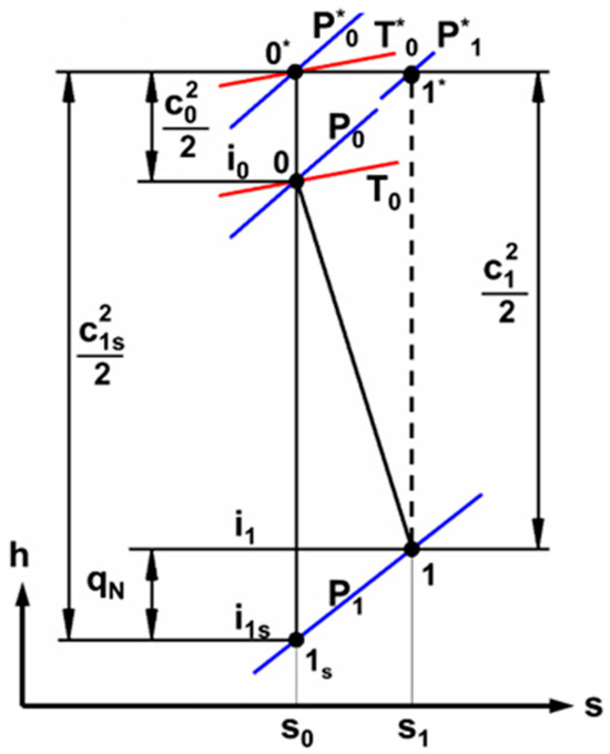
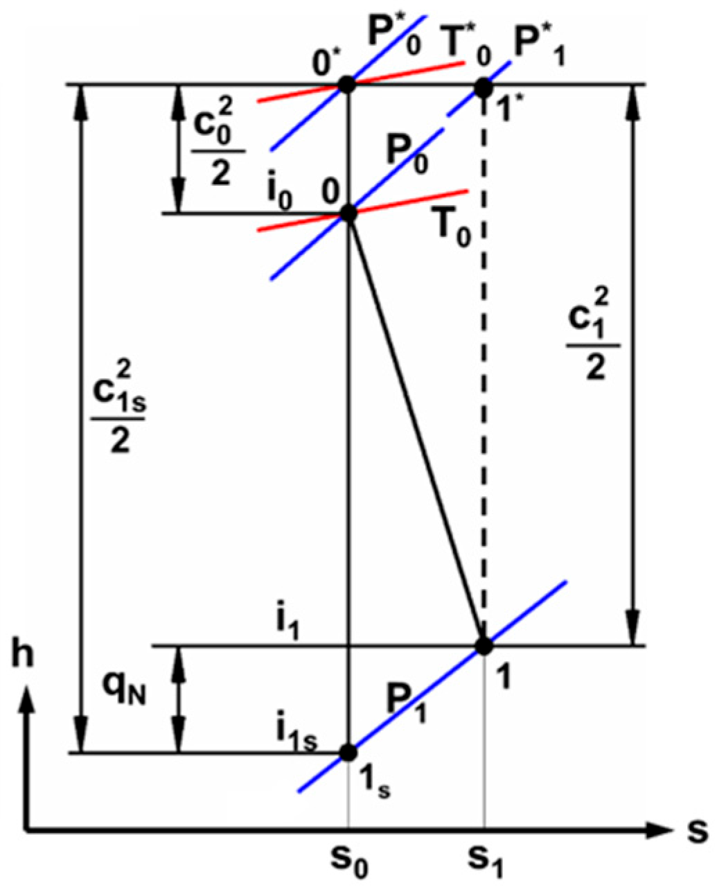
Figure 3 shows the process of expansion in the annular cascade for the midsection. According to the theory of turbomachines, the flow parameters with their symbols and subscripts are as follows:

Figure 3. Entropy growth in an expansion process in a stationary cascade in an h-s diagram.

• Subscripts: “0”—nozzle row inlet; “1”—nozzle row outlet; “s”—isentropic; “*”—total flow parameters;
• Symbols: C—velocity, m/s; P—pressure, Pa; T—temperature, K; i—static enthalpy, kJ/kg; h—total enthalpy, kJ/kg; s—entropy, kJ/(kg × K).

A commonly used indicator of energy conversion efficiency in a stator nozzle row is the total pressure loss coefficient $\xi$. According to Denton [10], accounting for losses in an adiabatic machine can be done by evaluating the entropy change. Expansion in a cascade is an irreversible process and is accompanied by an increase in entropy (Figure 3). The problem is that entropy cannot be measured directly, but the change can be estimated using two other parameters used in thermodynamics—pressure and temperature. The latter can be measured at specific points in the turbomachine flow path. Again, according to Denton, for adiabatic flow through a nozzle cascade, the entropy change Δs depends on the pressures measured at the inlet and outlet of the cascade (Figure 3).

For the nozzle row, the total pressure loss coefficient $\xi$ can be calculated [11]:

$$\xi ={\displaystyle \frac{P_0^{*}-P_1^{*}}{P_1^{*}-P_1}}$$

(4)

The total pressure loss coefficient $\xi$ is used by Beer [11] and Wingelhofer [5] to estimate the cascade entropy rise.

Before starting to calculate the variants, the quality of the mesh should be checked. It must have a high enough resolution near the walls of the annular cascade to solve the development of vortex structures in the interblade channels and subsequently make a qualitative comparative analysis. In addition to checking the dimensionless distance from the wall to the first grid cell center (Yplus) indicator, a mesh is generated in which the number of elements does not influence the values of the obtained results for the pressure loss coefficient $\xi$. Of course, generating a mesh with too many elements would increase the computation time. In Table 2, it can be seen that, beyond 1.8 million elements, it makes no sense to create a finer mesh. The mesh sensitivity results were obtained in the Mesh module for an unstructured mesh. A similar kind of comparison was performed for a structured grid in the Turbogrid module.

Table 2. The influence of the number of mesh elements on the value of the loss coefficient.

Variant No.	1	2	3	4	5
Node number	249,316	384,752	481,671	1,180,530	2,762,807
Element number	599,022	1,380,147	1,778,165	4,762,801	12,178,960
Loss coefficient  $\mathit{\xi }$, -	0.15	0.18	0.17	0.17	0.17

Modeling was done according to the rules for working with the ANSYS CFX software [12]. In the modeling process, two channels with two nozzle blades are created in order to be able to analyze the development of the secondary flows in the cascade flow path. The inlet, outlet, periodic boundary conditions, root wall, periphery wall and blade walls are defined. All calculations are performed with the turbulent SST model, using air (incompressible fluid) as the working fluid for BC Test 1 and superheated steam (IAPWS—IF97 [7]) as the working fluid for test group 2. In simulations of this type for a compressible fluid with high velocity (200 m/s), a subsonic outflow with M_max ≈ 0.5 is observed at the exit of the cascade. With similar gas parameters in the interblade channels, the Total Energy option is used, which is recommended for the considered working fluid [12]. This means that heat transfer and the work of viscous forces inside the working fluid are taken into account.

The boundary conditions of the first group (BC Test 1) refer to the variant with long blades (150 mm) and are taken from the work in [11]. In that study, the author, Dr. Beer, conducted experiments in a wind tunnel at TU-Wien, Austria, with a developed inlet boundary layer at the cascade inlet. With the help of precision measuring equipment, the turbulent intensity Tu at the inlet of the nozzle row was measured. For the simulation, a velocity $C$ distribution, turbulence intensity of 5% at the inlet, and atmospheric pressure at the outlet $P_0=0 \mathrm{P}\mathrm{a}$ were applied.

The second group of boundary conditions (BC Test 2.1, BC Test 2.2, BC Test 2.3) is for the comparative calculation variants targeting the short blades. Different operating scenarios with varying boundary conditions are applied to the cascade with a blade height of 64 mm. This group of boundary conditions was determined by the application of methodologies described in the specialized literature and is not considered in this report. To obtain the data for this group of boundary conditions, the one-dimensional design theory is used in combination with the application of the S1–S2 quasi-three-dimensional calculation methodology known from turbomachine theory [13,14].

Calculations with BC Test 1 boundary conditions show that the loss coefficient $\xi$ is lower for the CFIALE blade compared to CYLSLE. Therefore, it makes sense to examine the more efficient CFIALE blade in more detail. After that, an object in which to apply this blade is selected, and this is a steam turbine stage of a unit that is currently in operation in the power industry. For comparison, the same calculations are performed for the CYLSLE blade. The changes in the physical parameters at the input and the output are presented in Table 3 and visualized as contours in Figure 4.

Table 3. Summary table of boundary condition types and calculated loss coefficients.

			CYLSLE	CFIALE
	Inlet	Outlet	Loss Coefficient
Test 2.1	$P_0^{*}$ = var	$P_1$ = var	0.119	0.091
	$T_0^{*}$ = var
Test 2.2	$P_0^{*}$ = var	Gout = 10.8 kg/s	0.132	0.113
	$T_0^{*}$ = var
Test 2.3	$c_0$ = var	$P_1$ = var	0.113	0.088
	$T_0^{*}$ = var

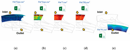
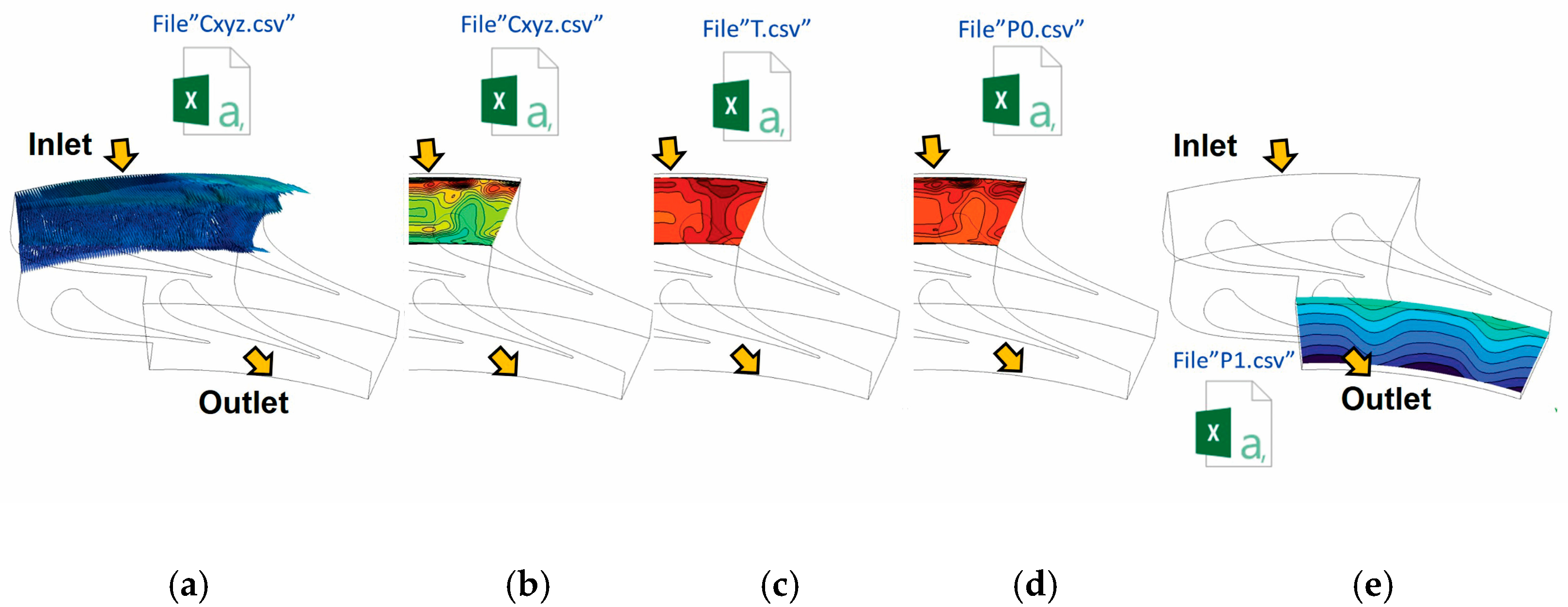
Figure 4. Boundary conditions set for cascade calculations: (a,b)—variable velocity field at inlet; (c)—variable total temperature at inlet; (d)—variable total pressure at inlet; and (e)—variable static pressure at cascade outlet. Arrows show flow direction.

The cascades were chosen to be tested under severe inlet vortex flow conditions, so variable pressure and temperature are applied, either separately with an inhomogeneous inlet velocity field or with variable outlet pressure, or a combination of these. Figure 4 shows the variation in these flow parameters, visualized with contours. The data for these boundary conditions are arranged in data CSV files (Comma-Separated Values files). They contain coordinates, as well as values of physical parameters ($P_0^{*}$, $T_0^{*}$, $c_0$, $P_1$), units, and names, presented according to the specifics of the syntax inherent to the CFD code in the CFX software [12].

Convergence of the equations must be monitored during the calculation process in the CFX-Solver module; variants without convergence are not analyzed further.

4. Results and Analysis

To facilitate the analysis, Table 3 presents the calculated data for the loss coefficient $\xi$ and the name of the test. In all calculations, lower loss coefficient values are observed for the CFIALE variant compared to CYLSLE. In BC Test 2.1, it is 24% lower; in BC Test 2.2, 17% lower; and in BC Test 2.3, 22% lower. In Table 3, G_out represents the superheated steam mass flow rate at the cascade outlet.

The next step is to find the reason for these lower loss coefficient values. Therefore, this report continues with an analysis of the results, which are divided into two groups: qualitative results and quantitative ones.

Given the large amount of generated data, the question arises as to how to compare the two cascades and how to assess their aerodynamic efficiency. One of the well-known ways these days is through the visualization of the vortex structures that are observed in the interblade channels. For this purpose, isosurfaces of vortex structures are used, which are calculated in the CFD-Post module. They are introduced to assess the development of secondary vortices. The Q-criterion is used to detect vortex structures. This method was applied in the research by Gao [15]. The symbols defined below are S_ij—magnitude of strain-rate tensor; Ω_ij—magnitude of vorticity tensor [15].

$$Q={\displaystyle \frac{1}{2}}\left({\mathsf{\Omega }}^2-{\mathrm{S}}^2\right)$$

(5)

$$S=\sqrt{2S_{ij}{S}_{ij}}, S_{ij}={\displaystyle \frac{1}{2}}\left({\displaystyle \frac{\partial U_i}{\partial x_j}}+{\displaystyle \frac{\partial U_j}{\partial x_i}}\right)$$

(6)

$$\mathsf{\Omega }=\sqrt{2{\mathsf{\Omega }}_{ij}{\mathsf{\Omega }}_{ij}}, {\mathsf{\Omega }}_{ij}={\displaystyle \frac{1}{2}}\left({\displaystyle \frac{\partial U_i}{\partial x_j}}-{\displaystyle \frac{\partial U_j}{\partial x_i}}\right)$$

(7)

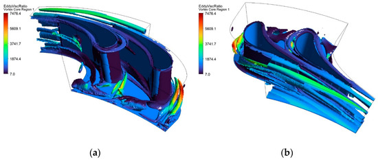
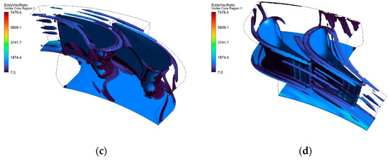
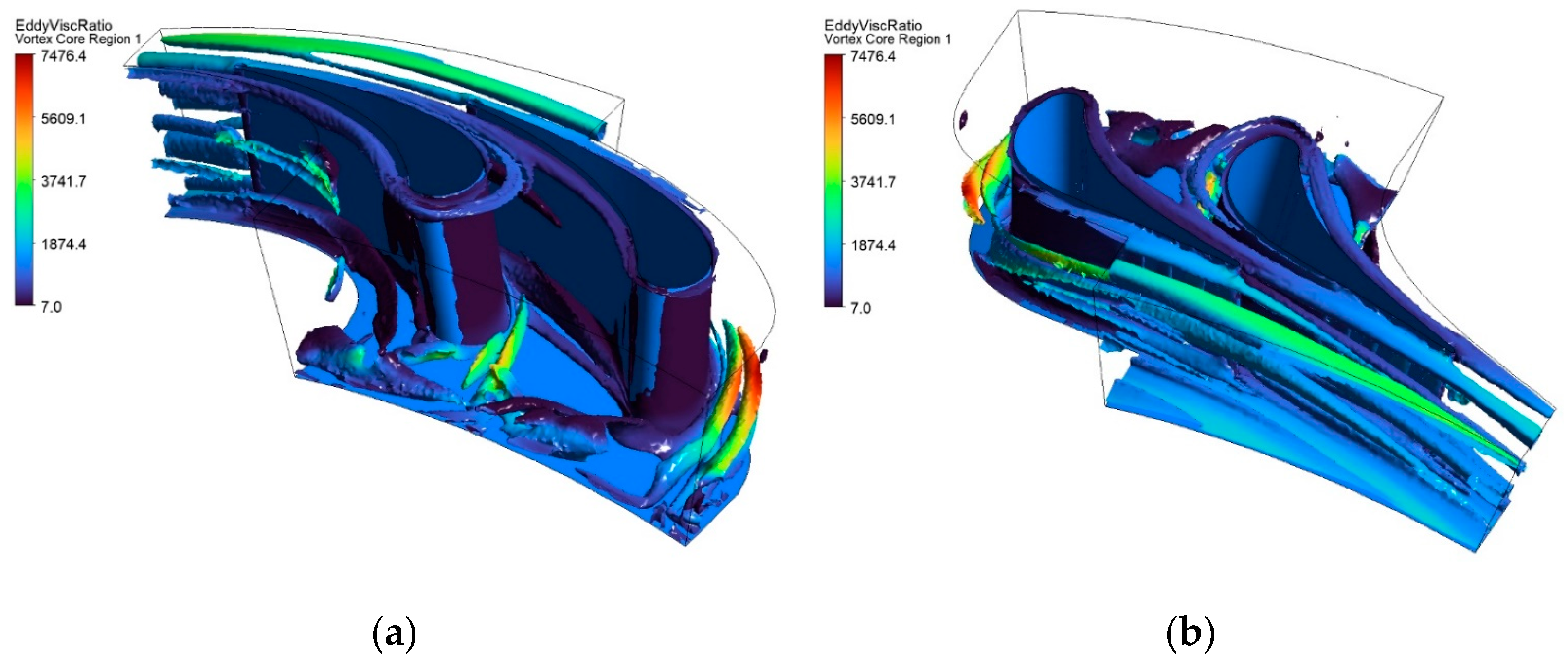
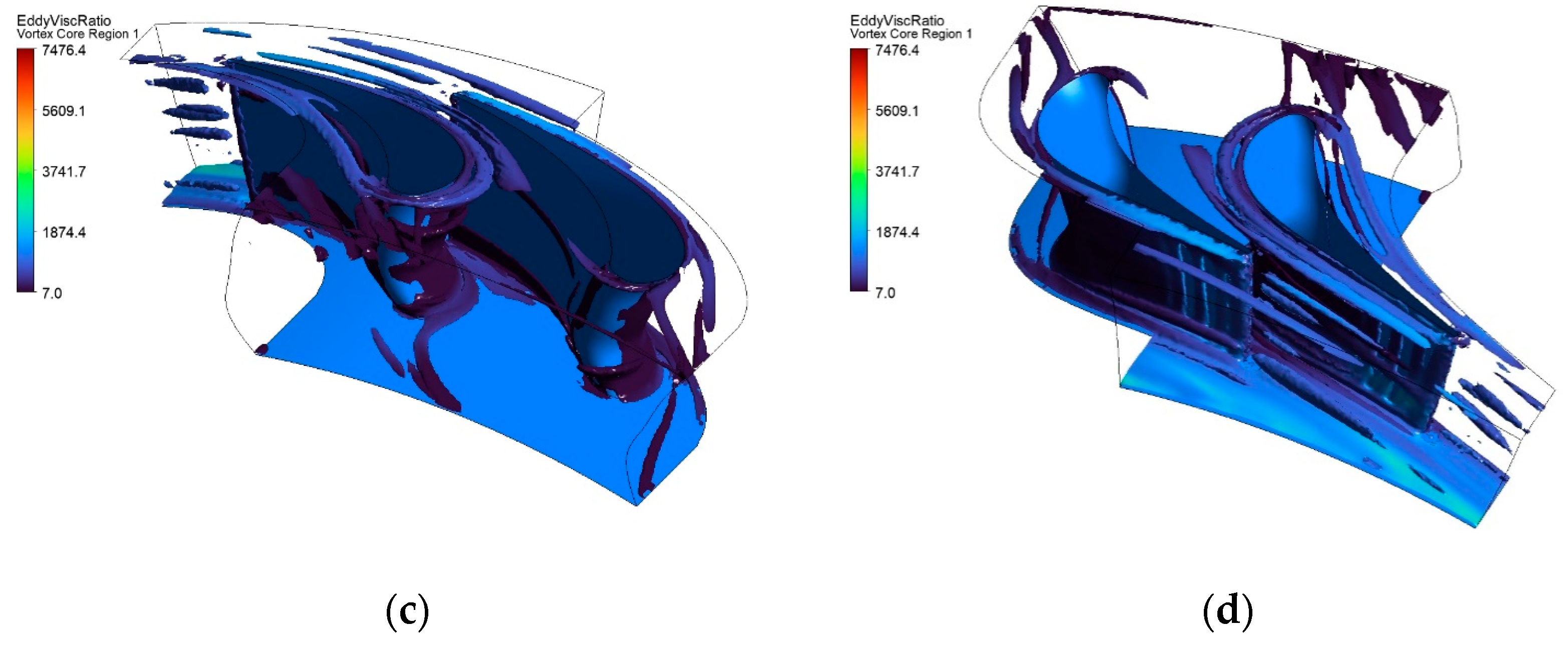
Vortices can also be visualized using the ratio of eddy viscosity to dynamic viscosity. This is also an applicable approach for the analysis of vortex structures in cascades [8] and is presented in Figure 5. This figure shows the development of the secondary flows for the CYLSLE blade cascade with $\xi$ = 0.119, Test 2.1, with inlet (Figure 5a) and outlet views (Figure 5b). A comparison can be made with the CFIALE variant, where the loss coefficient is $\xi$ = 0.088, Test 2.3, with inlet (Figure 5c) and outlet views (Figure 5d).

Figure 5. Vortex formation with eddy viscosity ratio visualization. (a,b) CYLSLE variant $\xi$ = 0.119 (Test 2.1); (c,d) CFIALE variant $\xi$ = 0.088 (Test 2.3).

The techniques described above make it possible to assess where the intensity of secondary vortices is low and to explain the reasons for the high efficiency of the CFIALE blade cascade. In the case of the cascade with CYLSLE blades, more intense vortex formation is observed at the root than at the peripheral wall (Figure 5a). The vortices rise up and continue to the cascade outlet (Figure 5b).

In the CFIALE variant, the passage vortex is generally weakened. The reason is the influence of the leading-edge shape on the region of origin of the horseshoe vortex at the root. In the lower half of the cascade, one leg, H_p, of the horseshoe vortex is missing (Figure 5c), which explains the low values of the pressure loss coefficient. At the periphery, the horseshoe vortex has been generated, but its magnitude is much smaller than that for the CYLSLE variant (Figure 5b,d).

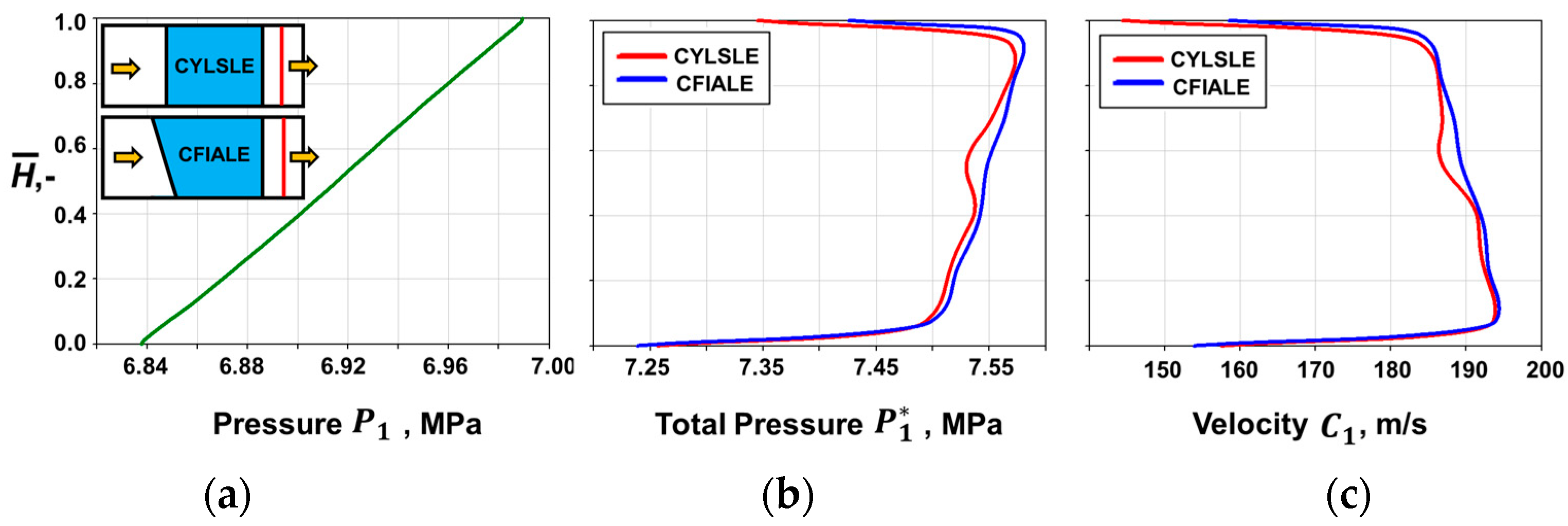
In order to analyze the quantitative results, a plane is defined in the cascade output at streamwise = 0.9 (the red line in Figure 6a). In this section, the calculated data for pressure $P_1$, total pressure $P_1^{*}$, and velocity $C_1$ are averaged. The outlet section is chosen to evaluate the effect of the three-dimensional changes of the blade on the flow. The flow input and output parameters are shown above in Figure 4. In the analysis, the relative height of the cascade $\overline{H}$ is defined, which represents the ratio of the height h of the blade at a certain radius to the maximum height, ℓ = 64 mm.

Figure 6. Comparison for the two blade variants in the outlet section, streamwise = 0.9, of the annular cascade by height: (a) static pressure $P_1$, (b) total pressure $P_1^{*}$ and (c) velocity $C_1$. Arrows show flow direction.

Figure 6a shows the variation in static pressure along the relative height $\overline{H}$ of the cascade at the outlet of the modeled fluid domain. There is an overlap between the pressure curves for the two cascade variants with CYLSLE and CFIALE blades because the same distribution of $P_1$ is set at the outlet (file “P1.csv” for Test 2.1 and Test 2.3). The pressure $P_1$ increases with relative height $\overline{H}$ because the flow entering the blade cascade in the root region encounters resistance due to the smaller pitch there, which causes the steam to be directed upwards. In the variant with the CFIALE blade, this is not observed due to the lean of the front edge in the axial and circumferential directions. At the sections in the periphery, the velocity is low (about 180 m/s), because the pitch is large, while at the base the velocity is higher (about 190 m/s). According to Table 1, the hub pitch is 85 mm, and the shroud pitch is 98 mm. Low velocity results in higher peripheral pressure. These are some of the physical relationships by which the velocity distribution over height is formed.

The quantitative comparative analysis from Figure 6b shows that, as a tendency, the output total pressure $P_1^{*}$ increases along the blade cascade height, but when comparing the two cascades with the CYLSLE and CFIALE blades in the section at $\overline{H}$ = 0.5, the following difference is observed: $∆P_1^{*}$ = 0.4%. In this section the total pressure is lower for the CYLSLE variant. The reason is vortex shedding, which is more intense in the CYLSLE variant compared to the CFIALE variant.

In Figure 6c, the velocity along the wall is equal to zero, but for better visibility, the range of $C_1$ for both variants is reduced from 0–200 m/s to 140–200 m/s. As can be seen from the same figure, the developed numerical models manage to capture the velocity gradient near the walls, the reason being the increased density of the mesh at the walls at the root ($\overline{H}$ = 0) and at the periphery ($\overline{H}$ = 1), which allows the boundary layer to be described correctly. The velocity profile of the exit velocity for the CYLSLE and CFIALE blade cascades presents a decreasing trend with increasing height $\overline{H}$. The velocity distribution is more uniform in the CFIALE variant compared to the CYLSLE variant. In the middle, $\overline{H}$ = 0.50, the velocity at the CYLSLE outlet cascade shows a drop due to the influence of the developed vortices (see Figure 5a on the blade right side, the vortex structure with the brightest red, yellow and green colors). In comparison with the CFIALE variant, a velocity difference of ${∆C}_1$ = 1.3% was found.

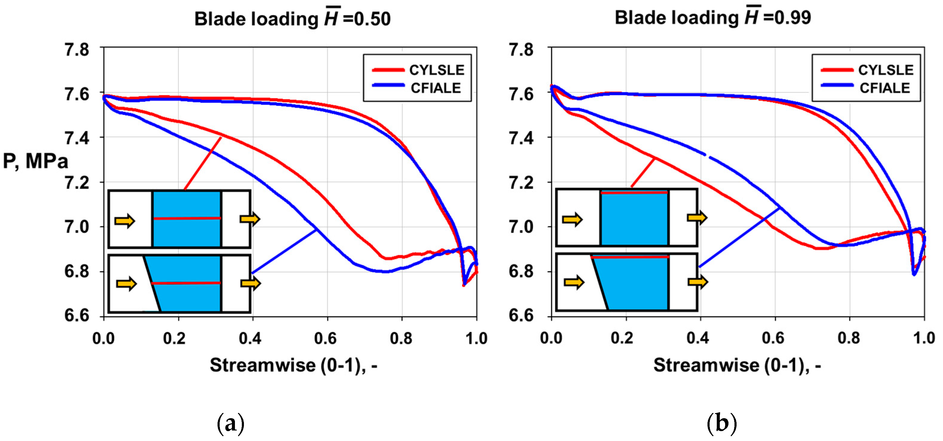
The quantitative analysis continues with the study of the influence of the blade’s three-dimensional shape modification on blade loading at two different cross-sections along the height of the annular cascade. Figure 7 shows the calculated static pressure distributions along the suction side (SS) and pressure side (PS) for BC Test 2.1 in two different sections: in the middle ($\overline{H}$ = 0.50) (a) and at the periphery ($\overline{H}$ = 0.99) of cascade (b).

Figure 7. The blade loading for the two blade variants for sections in the middle and at the periphery. Arrows show flow direction.

Near the leading edge, at a distance of 5% of the cascade width at the periphery ($\overline{H}$ = 0.99), the static pressure difference between the SS and the PS is calculated as ${∆P}_{CYLSLE}=P_{PS}-P_{SS}$, and the following differences are observed:

• For CYLSLE—${\overline{∆P}}_{CYLSLE}=1.2\mathrm{\%}$;

• For CFIALE—${\overline{∆P}}_{CFIALE}=0.6\mathrm{\%}$.

The calculations show that, at the periphery ($\overline{H}$ = 0.99), for the CFIALE variant, the difference $∆P$ after the leading edge is reduced by half, which is the location of development of the horseshoe vortex in the interblade channel. This causes a weakening of the secondary flows in the channel and a reduction in endwall losses.

A different picture is observed near the leading edge at a distance of 5% of the cascade width in the middle of the cascade ($\overline{H}$ = 0.50):

• For CYLSLE—${\overline{∆P}}_{CYLSLE}=0.8\mathrm{\%}$;

• For CFIALE—${\overline{∆P}}_{CFIALE}=1.2\mathrm{\%}$.

The calculations show that, in the middle, the differences in SS and PS at the airfoil leading edge are almost two times lower for both variants, maintaining the tendency for lower $∆P$ for CFIALE blades.

The midsection of the blades is equidistant from the boundary surfaces, and this results in less influence of the endwall, but vortices are present due to the inlet boundary condition, namely, the non-uniform velocity field, temperature, and pressure. This test serves to show how the two blade designs perform under these severe flow conditions. The test shows that the CFIALE blade shape is better than the CYLSLE blade design because of the smaller pressure differences, $∆P$, near the leading edge.

This concludes the quantitative evaluation of some of the phenomena occurring in the endwall zones of the blades.

5. Conclusions

In all considered operating scenarios, the calculated loss coefficient, $\xi$, is lower for the CFN INVERSE ARROW LE nozzle cascade modification compared to the CYL STRAIGHT LEAN LE cascade under the same conditions. The results are summarized in Table 4.

Table 4. Result summary of developed CFD models with three-dimensional blade designs.

	Incompressible Flow (Long Blade, ℓ = 150 mm)	Compressible Flow (Short Blade, ℓ = 64 mm)
	BC Test 1	BC Test 2.1	BC Test 2.2	BC Test 2.3
Loss coefficient $\xi$, - CYL STRAIGHT LEAN LE	0.1644	0.119	0.132	0.1128
Loss coefficient $\xi$, - CFN INV ARROW LE	0.1232	0.091	0.113	0.088

The loss coefficient is lowest ($\xi$ = 0.088) in the BC Test 2.3 boundary condition simulation with the CFN INVERSE ARROW LE blade with a length of 64 mm. This indicator of cascade efficiency is highest ($\xi$ = 0.1644) in BC Test 1 with the CYL STRAIGHT LEAN LE blade of 150 mm length.

The loss coefficient $\xi$ is calculated with formula (4), and the percent change can be calculated using the formula

$$\overline{\xi }={\displaystyle \frac{{\xi }_{CFIALE}-{\xi }_{CYLSLE}}{{\xi }_{CFIALE}}}\times 100,\%$$

(8)

After analyzing the data obtained and comparing them, the following conclusions can be drawn. The difference shows a decrease in the loss coefficient for the CFN INVERSE ARROW LE blade design as follows:

• In the first group of boundary conditions, BC Test 1 $\overline{\xi }$ = −25%;
• In BC Test 2.1, $\overline{\xi }$ = −31%; in BC Test 2.2, $\overline{\xi }$ = −17%; and in BC Test 2.3, $\overline{\xi }$ = −29%.

As an additional advantage, it can be pointed out that, with the CFN INVERSE ARROW LE blade, there is an equal and monotonous increase in the total pressure at the cascade outlet, while there is a monotonically decreasing exit velocity with no drop in distribution after the trailing straight edge. This can be useful in future research into turbine-stage operation because the outlet velocity profile of the stationary cascade is the inlet to the next cascade that rotates.

The differences in static pressure are two times smaller for the CFN INVERSE ARROW LE variant compared to the CYL STRAIGHT LEAN LE variant near the leading edge in the peripheral zones. This means that end losses are reduced but not eliminated.

In conclusion, it should not be forgotten that, despite the successes achieved so far in the field of CFD modeling, numerical simulations cannot completely replace physical experiments. In the future, the team plans to perform calculations with the addition of a rotating fluid domain to the model to determine the efficiency of the turbine stage and a multi-stage flow section. The use of other turbulence models and LES simulation could further clarify the efficiency enhancement mechanisms in the CFN INVERSE ARROW LE blade row. The present study may help prepare a model for an experimental study in a wind channel and direct attention to more efficient blade shape designs.

References

- Cofer, J.I. Advances in Steam Path Technology. J. Eng. Gas Turbines Power. 1996, 118, 337–352. [Google Scholar] [CrossRef] [Scilit][Green Version]
- Leyzerovich, A. Steam Turbines for Modern Fossil-Fuel Power Plants, 1st ed.; River Publishers: Gistrup, Denmark, 2007; 350p. [Google Scholar] [CrossRef] [Scilit]
- Kawai, T. Effect of Combined Boundary Layer Fences on Turbine Secondary Flow and Losses. JSME Int. J. Ser. B 1994, 37, 377–384. [Google Scholar] [CrossRef] [Scilit]
- Vogt, H.; Zippel, M. Sekundärströmungen in Turbinengittern mit geraden und gekrümmten Schaufeln; Visualisierung im ebenen Wasserkanal. Forsch. Ingenieurwesen 1996, 62, 247–253. [Google Scholar] [CrossRef] [Scilit]
- Wingelhofer, F. Neue Kriterien zur Auslegung dreidimensionaler Beschaufelungen von Axialturbinen. Dissertation. 2003. Available online: https://repositum.tuwien.at/handle/20.500.12708/12130?mode=full (accessed on 1 September 2026).
- Haller, B.; D’Ovidio, A.; Henson, J. Development of improved reaction technology blading (RTB LAR) for large steam turbines. In Proceedings of the ASME 2019 Power Conference, Salt Lake City, UT, USA, 15–18 July 2019; V001T08A001; ASME: New York, NY, USA, 2019. [Google Scholar] [CrossRef] [Scilit]
- ANSYS. ANSYS CFX-Solver Theory Guide; ANSYS Release 2025R1; ANSYS: Canonsburg, PA, USA, 2025. [Google Scholar]
- Menter, F.R. Turbulence Modelling for Technical Flows. NAFEMS Int. J. CFD Case Stud. 2006, 5, 41–49. [Google Scholar] [CrossRef] [Scilit]
- Menter, F. Improved Two-Equation k-ω Turbulence Models for Aerodynamic Flows. NASA Technical Memorandum 103975. October 1992. Available online: https://arc.aiaa.org/doi/10.2514/6.1993-2906 (accessed on 1 September 2026).
- Denton, J. Loss Mechanisms in Turbomachines. In Proceedings of the ASME 1993 International Gas Turbine and Aeroengine Congress and Exposition, Cincinnati, OH, USA, 24–27 May 1993; V002T14A001; ASME: New York, NY, USA, 1993. [Google Scholar] [CrossRef] [Scilit]
- Beer, W. Optimisation of a Compound Lean Turbine Blade in a Linear Cascade. Doctoral Dissertation, TU Wien, Wien, Austria, 2008. Available online: https://repositum.tuwien.at/handle/20.500.12708/11188 (accessed on 1 September 2026).
- ANSYS. ANSYS CFX-Pre User’s Guide; ANSYS Release 2025R1; ANSYS: Canonsburg, PA, USA, 2025. [Google Scholar]
- Wu, C. General Theory of Three-Dimensional Flow in Subsonic and Supersonic Turbomachines of Axial-, Radial-, and Mixed-Flow Types. 1952. Available online: https://asmedigitalcollection.asme.org/fluidsengineering/article-abstract/74/8/1363/1144712/A-General-Theory-of-Three-Dimensional-Flow-in?redirectedFrom=fulltext (accessed on 1 September 2026).
- Terziev, A.; Potashev, A.; Potasheva, E.; Khisameev, I.; Valeeva, Y.; Beloev, H.; Iliev, I. Quasi-three-dimensional modeling as an effective tool for studying flows in turbomachines. IOP Conf. Ser. Earth Environ. Sci. 2024, 1380, 012020. [Google Scholar] [CrossRef] [Scilit]
- Gao, Y.; Liu, Y. A flow model for tip leakage flow in turbomachinery using a square duct with a longitudinal slit. Aerosp. Sci. Technol. 2019, 95, 105460. [Google Scholar] [CrossRef] [Scilit]
Disclaimer/Publisher’s Note: The statements, opinions and data contained in all publications are solely those of the individual author(s) and contributor(s) and not of MDPI and/or the editor(s). MDPI and/or the editor(s) disclaim responsibility for any injury to people or property resulting from any ideas, methods, instructions or products referred to in the content. |
© 2026 by the authors. Licensee MDPI, Basel, Switzerland. This article is an open access article distributed under the terms and conditions of the Creative Commons Attribution (CC BY) license.