Analysis of Z-Wave RSSI: Simulation-Based Modeling and Real-World Data ^†

Abstract

This paper investigates the behavior of the Received Signal Strength Indicator (RSSI) in Z-Wave networks through a comparison between simulation-generated and experimentally measured data. A prototype star-topology Z-Wave network was implemented and RSSI values were measured at distances from 1 m to 5 m with a gradually increasing number of active end devices in a laboratory environment. In parallel, a software simulation environment was used to reproduce the same topology and generate RSSI values under different propagation assumptions. In order to compare the results obtained from real and simulated environments, the average deviation between the range of measured values for RSSI was calculated. The experimental results show that the RSSI values from the simulation product follow the trend of deteriorating values with increasing distance between the central and end devices. The calculated average deviation between the range of RSSI values in real and simulated environments shows that the simulated results are closest to the real ones at an exponential coefficient n ≈ 2, and the calculated deviation is from 2 dBm to 2.3 dBm. The results obtained support the evaluation of the simulation model and show its potential for studying signal behavior and aiding the design of reliable Z-Wave-based Internet of Things environments.

1. Introduction

Z-Wave devices are engineered for low power consumption, which is crucial for battery-operated devices such as sensors, as it extends operational lifespans and reduces maintenance costs. The versatility of Z-Wave technology enables its application across various sectors, including remote water metering systems, grid load management, gas leak detection, predictive maintenance, and smart energy management systems. These applications facilitate real-time energy consumption tracking, resulting in a 20% reduction in energy loss and enhanced network stability [1]. Furthermore, Z-Wave is utilized in industrial control systems designed for process automation and control, highlighting its adaptability within Internet of Things (IoT) ecosystems where energy efficiency and reliable communication are paramount. This technology not only supports efficient resource management but also contributes to the mitigation of environmental impacts associated with energy consumption [2,3,4].

Received Signal Strength Indicator (RSSI) values in Z Wave can be used to investigate the connection status and potential causes of communication interruptions. This is a key indicator of the available sources of interference and objects that cause the signal to fade. This indicator can be used for optimal placement of nodes in the network to achieve complete and stable wireless signal coverage. This parameter is also useful for detecting intentional generation of malicious jamming signals. Other uses of RSSI include determining the reliability of a mesh Z-Wave network, optimizing the battery life of nodes, and preventing asymmetric connections [5].

This paper compares the RSSI values obtained from end sensor nodes in a simulated Z-Wave network with those from a real Z-Wave sensor network. The objective is to assess the accuracy of the simulation results by comparing them with real-world measurements. Through data analysis and comparison, this study aims to provide insights into the performance of Z-Wave networks, which can contribute to the optimization of future IoT system design and deployment. These findings are particularly relevant to the field of electrical engineering, as they can aid in the development of more efficient wireless communication systems, enhance network reliability, and support the advancement of smart grid and automation technologies.

2. Related Works

A few studies have explored the use of RSSI in wireless and IoT environments. For instance, in [6] analyzes different digital filters—such as simple moving average, alpha trimmed mean, and Kalman filters—to process RSSI data, aiming to reduce noise and improve data proximity, thereby facilitating more dependable signal strength assessments in IoT applications.

In [7] a prototype development is presented for studying the quality of the wireless connection with the study of the measured RSSI values based on the IEEE 802.11 standard in an IoT environment. The study in [8] presents the development of an experimental prototype based on a wireless IoT network with total dissolved solids for monitoring the quality of estuarine waters in support of the fisheries sector. The calibration of the system in terms of the transmitting and receiving signal is carried out based on the measured values for RSSI.

Additionally, in [9] machine learning-based models are proposed to predict RSSI in urban mesh networks, highlighting the influence of factors like distance and obstructions on signal strength, which is crucial for optimizing network design and deployment.

One of the applications of RSSI is performing localization of mobile indoor nodes, as this process can be influenced by various factors such as the behavior of radio waves, the nature of the experimental environment, or the available infrastructure. In [10], an experimental localization of indoor nodes in a wireless sensor network for IoT using RSSI with a multilateration technique is presented. Factors that influence the determination of the preliminary required operating power for better localization are presented. An increasingly popular method for accurately locating indoor nodes is RSSI fingerprinting, as described in [11,12], which incorporates artificial intelligence methods, as demonstrated in [13].

The calculation of RSSI values can also be used to detect jamming attacks against wireless IoT systems as presented in [14], where a threshold value for signal strength is used as a guideline for indicating an attack. The values of the measured RSSI levels can be used as a reference when choosing the most suitable IoT standard for implementation during design depending on the characteristics of the building in which the network will be implemented as presented in [15].

Most of the research considered focuses on applications different from the direct comparison between simulated and experimentally measured RSSI values in a Z-Wave prototype network, which is the focus of this research.

3. Received Signal Strength Indicator

The RSSI is a crucial metric in wireless communication systems, including Z-Wave networks, as it quantifies the power level of a received signal, typically expressed in decibels relative to one milliwatt (dBm). Accurate RSSI measurements are essential for assessing signal quality, optimizing network performance, and ensuring reliable connectivity in IoT and smart home applications. Various studies have explored methods to enhance the accuracy and reliability of RSSI readings.

In [6], filtering methods such as the simple moving average, alpha trimmed mean, and Kalman filter are examined to improve the stability of RSSI-based observations. In [7], RSSI is used in an experimental IoT prototype as an indicator of communication behavior in a practical deployment. In [8], machine learning techniques are applied for RSSI prediction, showing that signal strength can also be modeled computationally under varying conditions.

Other studies use RSSI in localization, fingerprinting, and security-related scenarios. In [9], RSSI is considered in the context of indoor localization, while [11,12] investigate RSSI-based fingerprinting approaches for spatial identification and positioning. In [10], signal-related indicators are employed for detecting jamming behavior. Additional works such as [13,14,15] further confirm that RSSI is strongly influenced by environmental conditions and remains an important parameter for wireless performance assessment.

Although these studies demonstrate the broad applicability of RSSI in wireless research, they do not focus specifically on validating simulation-generated RSSI values against real measurements in a controlled Z-Wave topology. In contrast, the present work compares RSSI values obtained from a developed Z-Wave simulation environment with measurements collected from a real prototype network under comparable topological and distance conditions.

The large range of areas in which measured RSSI values are used show that it is an important metric to study. The RSSI is measured in decibels per milliwatt (dBm) using Equation (1):

RSSI (dBm) = Pt (dBm) – 10·n·log10(d) + Loss,

(1)

• RSSI (dBm)—the signal level in decibels relative to one milliwatt (dBm);
• Pt (dBm)—the power of the transmitted signal in decibels relative to one milliwatt;
• d is the distance between the transmitter and receiver (in meters);
• n is the exponential coefficient that depends on the environment: n ≈ 2 for open space; n ≈ 3 for moderately built-up areas; n ≥ 4 for densely populated or enclosed spaces.
• Loss is the additional loss that may be due to specific conditions, such as walls, concrete barriers, and other obstacles.

Equation (1) is implemented within the simulation environment to compute RSSI for end devices in a simulated Z-Wave network topology.

4. Topology Configuration in Simulation and Real Environment

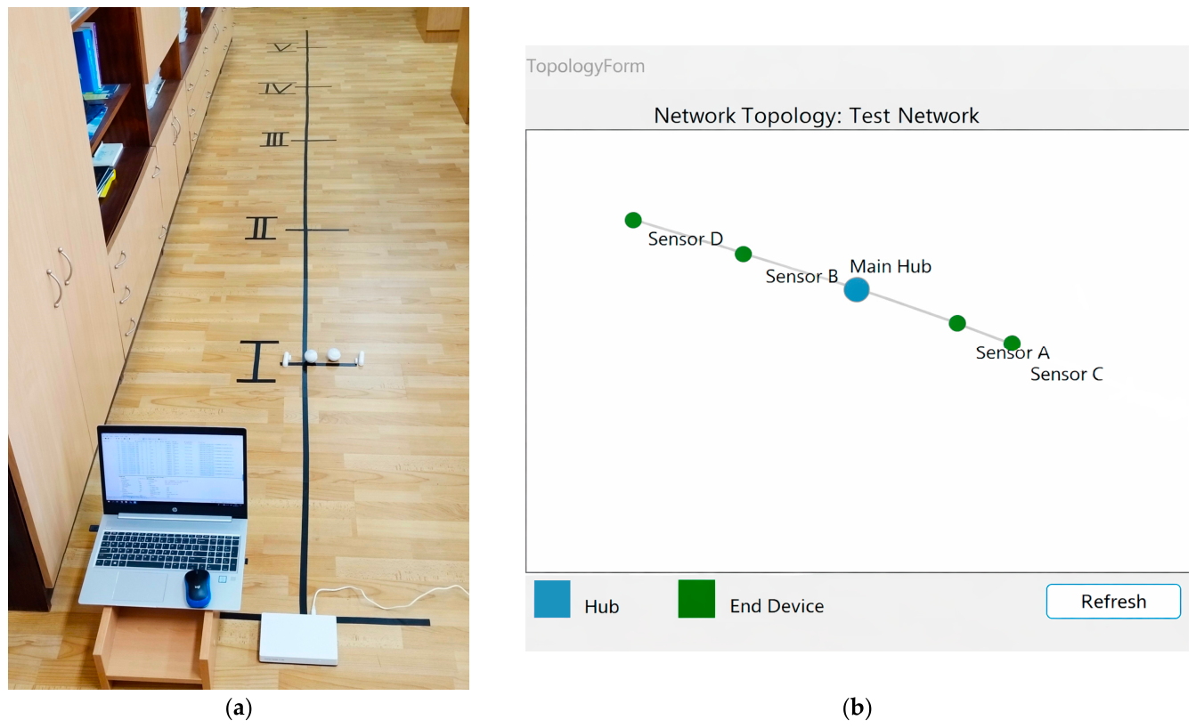
For the purposes of the experimental study set out in the current paper, a prototype Z-Wave network has been realized in which the devices are connected in a star topology. The device that implements the main hub functionalities is Home Center 3 Lite model HC3L-001, to which two Door/Window Sensors 2 model FGDW-002 and two Motion Sensors model FGMS-001 are sequentially connected. All of the used hardware for realizing real Z-Wave network are manufactured by Fibaro, Wysogotowo in Poland. The network has been set up in a laboratory environment at the Technical University—Varna. The connection topology is presented in Figure 1. The RSSI values have been measured using the Z-Wave sniffer ZME_UZB1 manufactured by Z-Wave.Me and the Z-Wave Zniffer software version 4.60.173. The RSSI values have been measured sequentially over 1 m to 5 m between the sensors and the central device. A sample of 10 RSSI values has been taken at each distance of the end nodes, and the arithmetic mean of these measurements is presented for a more accurate reflection of the values. The selected sample consists of 10 measurements because it covers all possible changes in the measured RSSI values for the respective distance. For all distances, experiments were performed with a gradual increase in the number of simultaneously connected devices in the Z-Wave network, adding end devices from 1 to 4.

After establishing the real prototype topology and its simulated counterpart, the next step is to use the software analysis module to generate the RSSI-based simulation results.

The developed at Technical University—Varna simulator is not limited to the generation of topology and signal graphs alone but represents a structured software environment in which the Z-Wave network is first configured and only afterwards analyzed. Before the RSSI analysis stage is reached, the user passes through several preparatory steps related to the creation of the simulated network. These include defining the network itself, configuring the central hub, and adding the corresponding nodes and end devices. In this way, the logical structure of the network is constructed so that it reflects the intended experimental scenario.

To ensure comparability between the results of the measured RSSI values in a real environment and simulation, it is necessary to implement experiments under the same conditions. In this case, a Z-Wave network is implemented in the simulation environment in which one main hub is configured, to which up to 4 end sensor nodes are connected (Figure 1). To implement experiments comparable to those in a real environment, end sensor nodes are added sequentially to the network from 1 to 4. For each experiment, a simulation was performed to calculate the RSSI values for each end node, considering the distance between the central and end devices from 1 to 5 m. The implemented simulation experiments reflect the RSSI values at three different values of the exponential coefficient that depends on the environment, n, presented in Equation (1).

The simulation experiments were carried out on a computer running Microsoft Windows 11 Pro. The system was equipped with an 11th Gen Intel Core i5-11300H processor operating at 3.10 GHz, 8 GB of RAM, and Intel Iris Xe Graphics. This hardware platform was used for the execution of the developed Z-Wave simulation environment and for generating the graphical and tabular outputs employed in the analysis.

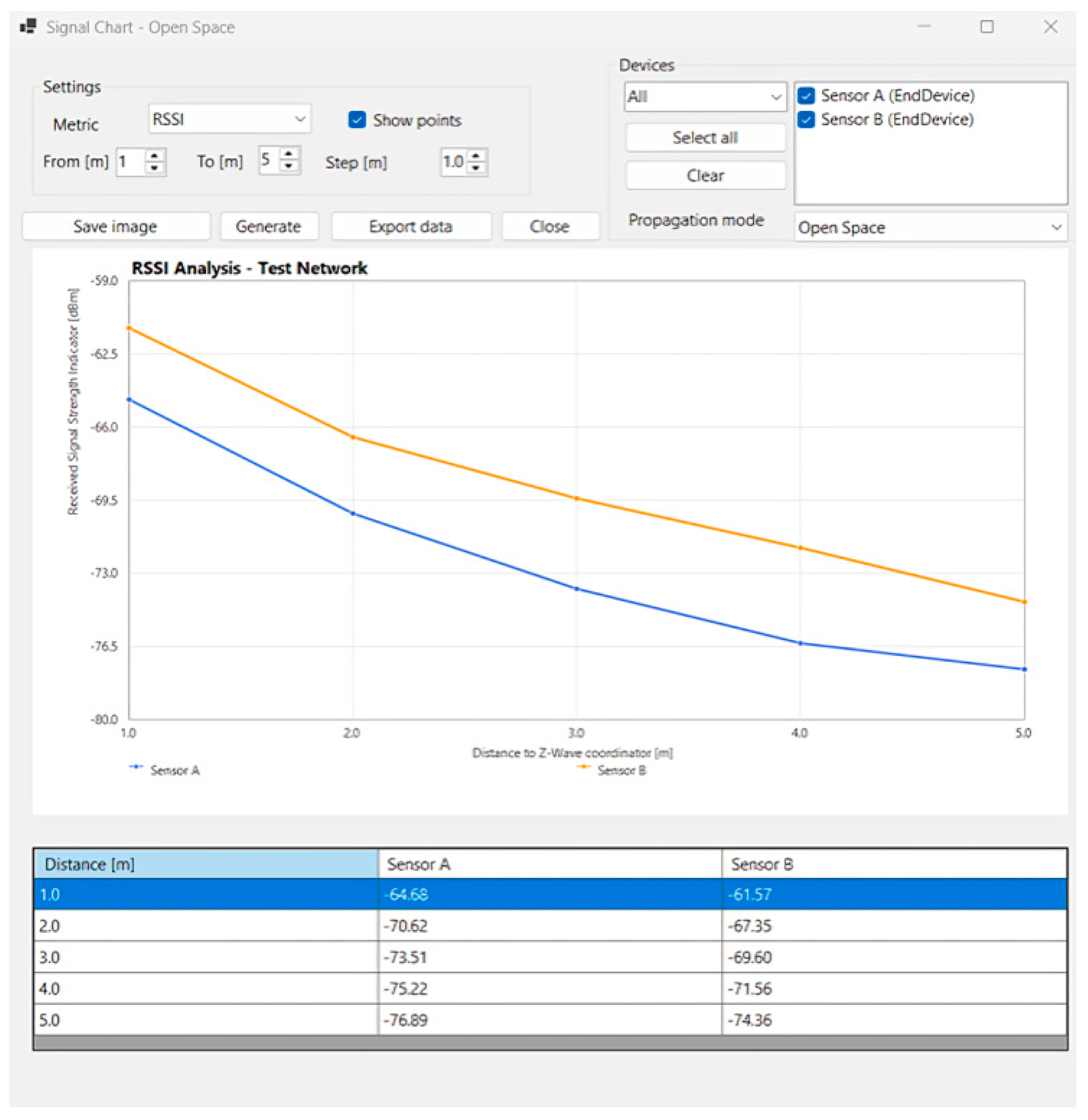
After the network has been created, the simulator proceeds to the analysis stage, where the configured topology is used as the basis for generating signal-related results. The RSSI analysis module shown in Figure 2 represents the main working environment for this part of the study. Through this module, the user can select the signal metric to be examined, define the distance range and simulation step, choose the participating devices, and apply the corresponding propagation mode. This makes it possible to examine the signal behavior under different assumptions while preserving the same network structure.

A practical advantage of this module is that it combines configuration, visualization, and data representation within a single screen. The simulator generates RSSI-versus-distance curves for the selected devices and, at the same time, presents the corresponding numerical values in tabular form below the graph. This makes the analysis easier to follow and supports subsequent processing of the obtained results. In addition, the interface includes options for saving the generated image and exporting the numerical data, which further supports the use of the simulator as an experimental and analytical tool rather than only a demonstrational environment.

The possibility to switch between different propagation modes is particularly important for the purposes of the present study. In the developed simulator, three propagation modes are considered: open space, moderate indoors, and dense indoors. These modes correspond to different values of the path-loss exponent $n$, with values around $n\approx 2$ for open space, $n\approx 3$ for moderate indoor conditions, and $n\ge 4$ for dense indoor environments. This is especially relevant when comparing the simulation output with the measurements obtained from the real Z-Wave prototype network, since such a comparison requires not only a fixed topology, but also an appropriate signal propagation model.

5. Experimental Results and Discussion

To compare the RSSI values measured in real and simulated environments, four groups of experimental studies were performed, considering the number of available physical end-sensor nodes.

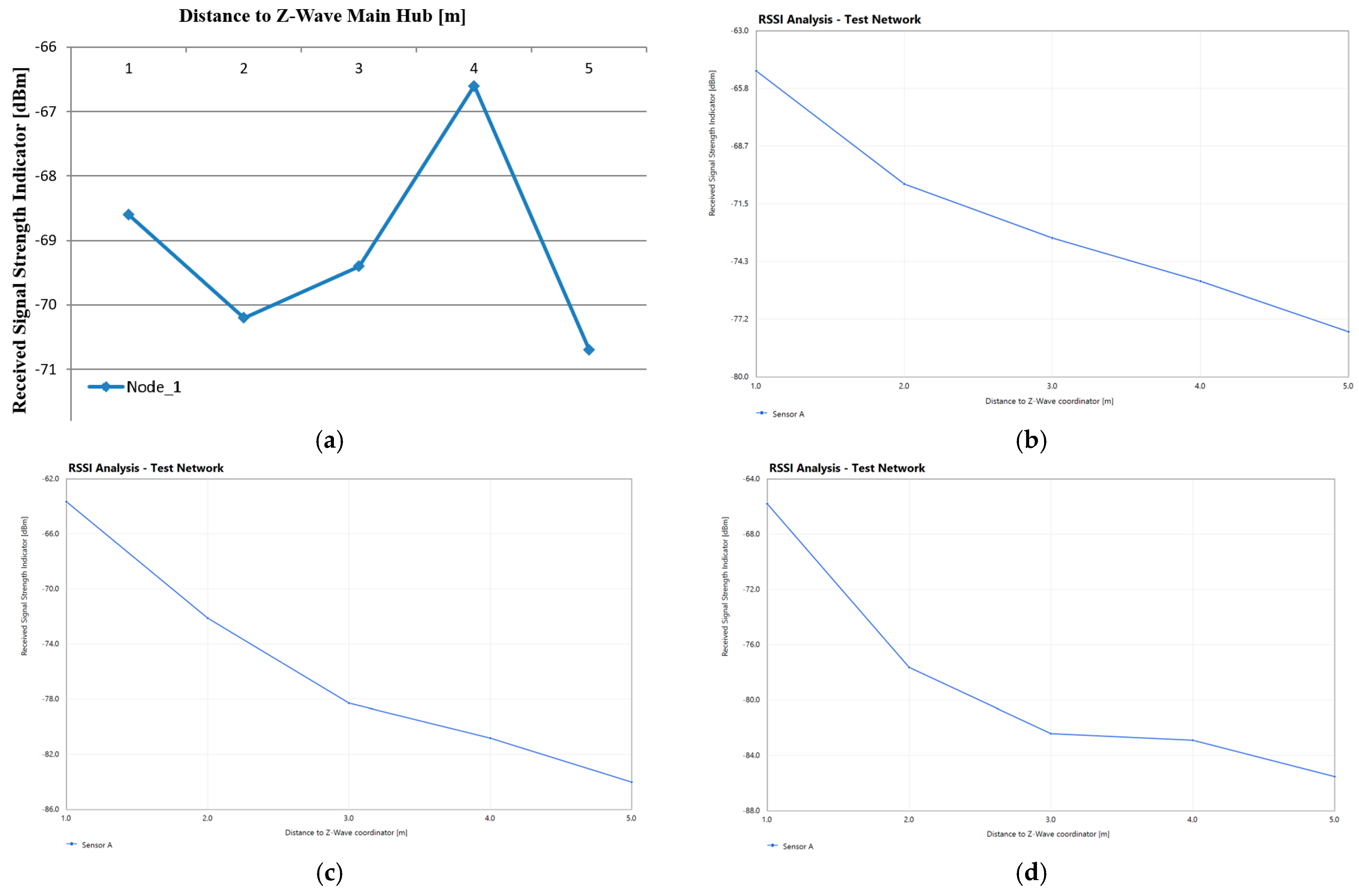
In the first group of experiments, the RSSI values with one connected end device in a real and simulated network are presented (Figure 3). The simulator presents 3 experimental results, each with a different value of “n” (exponential coefficient). A larger value of “n” simulates the presence of more objects in the environment in which the signal is propagated, which degrades its quality. From the presented results, the trend of changing RSSI values in real and simulated environments with increasing distance between the central and end device remains the same. This trend shows that the signal quality deteriorates with increasing distance between the central and end device. With one end device connected to the network in the real environment, the RSSI values change in the range from −66 dBm to −71 dBm. In a simulation environment, RSSI values at n ≈ 2 change in the range from −65 dBm to −78 dBm, at n ≈ 3 change in the range from −64 dBm to −84 dBm, at n ≥ 4 change in the range from −67 dBm to −86 dBm.

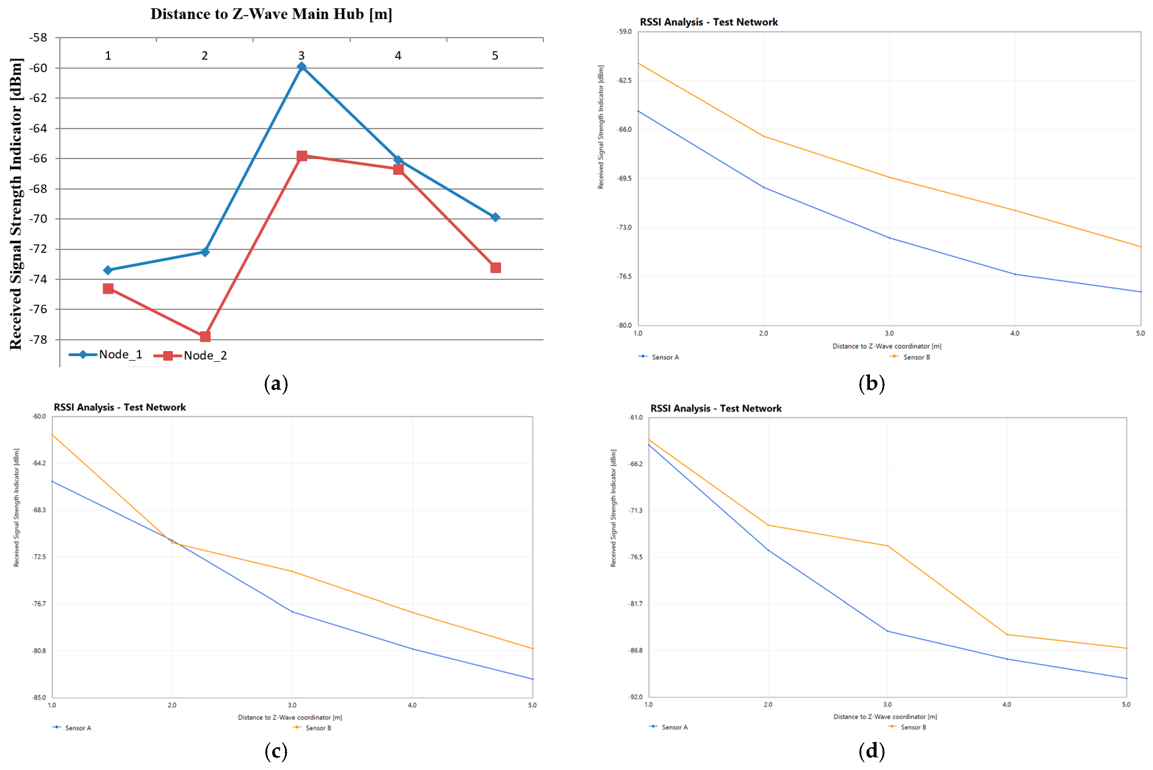
In the second group of experiments, the RSSI values with two simultaneously connected end devices in a real and simulated network are presented (Figure 4). Experimental results are presented through the simulator for each of the values of “n”. The presented results show that in a real environment, the RSSI values remain close without major differences for the two devices with increasing distance between the central and the end device. This is because at this stage of the experiments, two identical sensor nodes with identical hardware parameters and transmission gain of the antenna are connected to the network in a laboratory environment. For Node_1, the RSSI values change in the range from −60 dBm to −75 dBm, and for Node_2 in the range from −66 dBm to −79 dBm. According to the results from the simulation environment, with increasing distance between the central and end devices, the RSSI values deteriorate for different values of “n”. In the simulation environment, the RSSI values at n ≈ 2 for Sensor A change in the range from −65 dBm to −77 dBm, and for Sensor B in the range from −60 dBm to −74 dBm. At n ≈ 3 for Sensor A the values change in the range from −65 dBm to −83 dBm, and for Sensor B in the range from −62 dBm to −80 dBm. At n ≥ 4 for Sensor A the values change in the range from −64 dBm to −89 dBm, and for Sensor B in the range from −63 dBm to −86 dBm.

In the third group of experiments, the RSSI values with three simultaneously connected end devices in a real and simulated network are presented (Figure 5). The presented results show that in a real environment, there are no large differences in the measured RSSI values for the three devices with increasing distance between the central and the end devices. This is because the devices are in a laboratory environment without a large load on the network. For Node_1, the RSSI values change in the range from −60 dBm to −71 dBm, for Node_2 in the range from −61 dBm to −71 dBm, and for Node_3 in the range from −61 dBm to −66 dBm. The results from the simulation environment show that the trend of deterioration of RSSI values with increasing distance between the central and end devices, for different values of “n”, is maintained. In a simulation environment, the RSSI values at n ≈ 2 for Sensor A change in the range from −65 dBm to −77 dBm, for Sensor B in the range from −61 dBm to −73 dBm, and for Sensor C in the range from −64 dBm to −76 dBm. At n ≈ 3 for Sensor A the values change in the range from −65 dBm to −83 dBm, for Sensor B in the range from −62 dBm to −79 dBm, and for Sensor C in the range from −66 dBm to −85 dBm. At n ≥ 4 for Sensor A the values change in the range from −62 dBm to −87 dBm, for Sensor B in the range from −58 dBm to −90 dBm, and for Sensor C in the range from −65 dBm to −86 dBm.

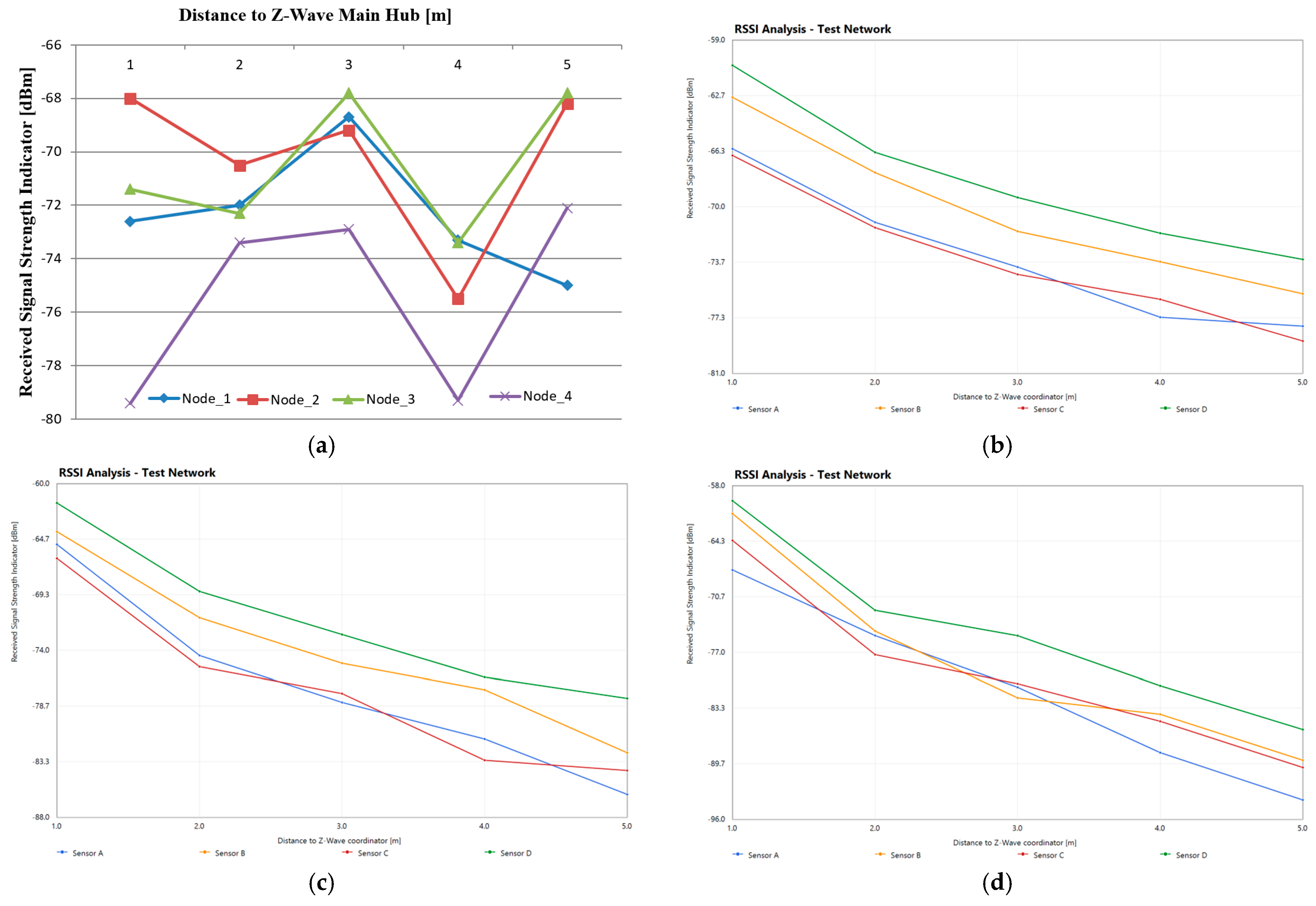
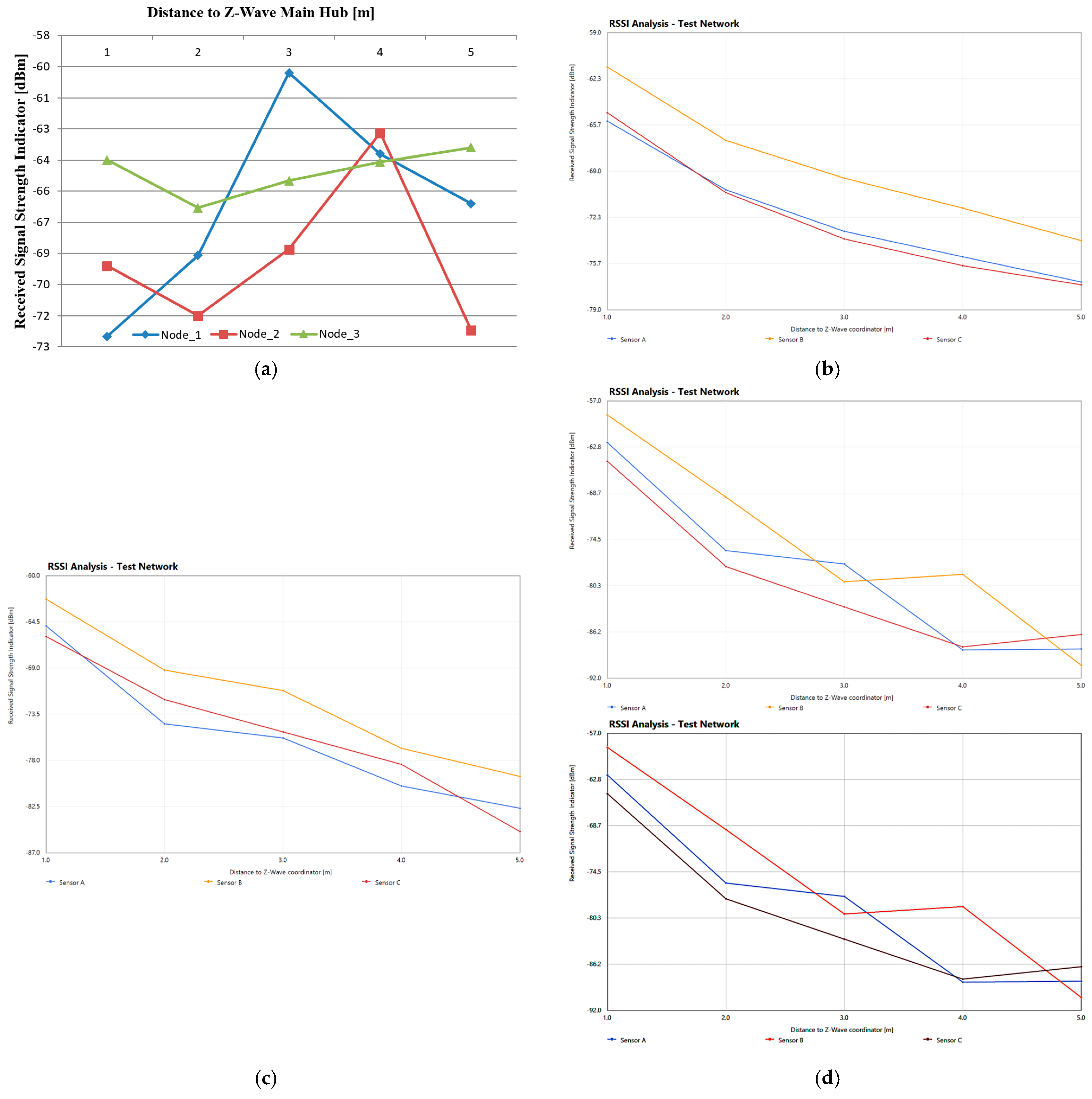
The fourth group of experiments presents the RSSI values with four simultaneously connected end devices in a real and simulated network (Figure 6). The results in a real environment show that the RSSI values for some of the devices increase by increasing distance between the central and end devices, while for another part they remain almost constant. This is due to the load on the communication medium and the transmission gain of the sensor nodes antennas. For Node_1, the RSSI values change in the range from −69 dBm to −75 dBm, for Node_2 in the range from −68 dBm to −76 dBm, for Node_3 in the range from −68 dBm to −73 dBm, and for Node_4 in the range from −72 dBm to −79 dBm.

The results from a simulation environment confirm that the trend of deterioration of RSSI values with increasing distance between the central and end devices, for different values of “n”, is maintained. In a simulation environment, the RSSI values at n ≈ 2 for Sensor A change in the range from −66 dBm to −77 dBm, for Sensor B in the range from −63 dBm to −76 dBm, for Sensor C in the range from −67 dBm to −78 dBm, and for Sensor D in the range from −61 dBm to −74 dBm. At n ≈ 3 for Sensor A the values change in the range from −65 dBm to −85 dBm, for Sensor B in the range from −64 dBm to −82 dBm, for Sensor C in the range from −66 dBm to −84 dBm, and for Sensor D in the range from −62 dBm to −78 dBm. At n ≥ 4 for Sensor A the values change in the range from −67 dBm to −94 dBm, for Sensor B in the range from −60 dBm to −89 dBm, for Sensor C in the range from −64 dBm to −90 dBm, and for Sensor D in the range from −59 dBm to −85 dBm.

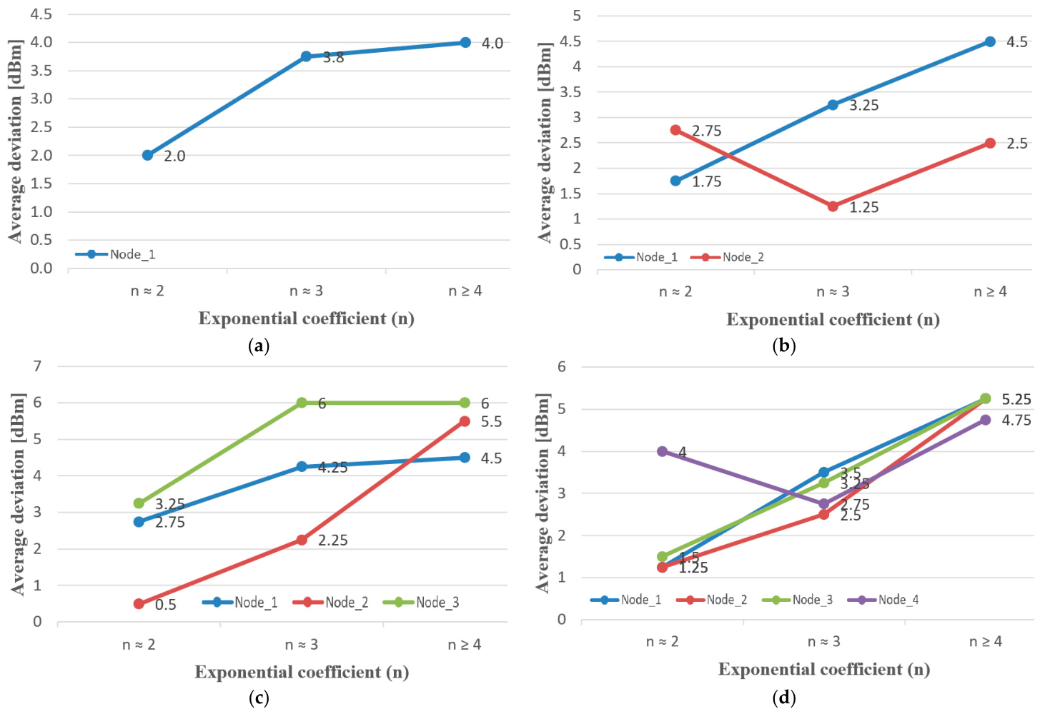
Based on the experiments conducted in real and simulated environments, the average deviation between the range of obtained RSSI values in real and simulated environments was calculated using Excel. The average deviation between the range of the obtained results with the different network configurations with end devices from 1 to 4 is reflected. The average deviation between the range of the simulated RSSI results with different values of “n” and those measured in real environments is presented (Figure 7). They show that with an increase in the number of simultaneously connected devices in the network, the deviation of the simulated results from the real ones increases. This is also noticeable when the values for “n” increase, with high values for the deviation between the results from the real and simulated Z-Wave network tending to remain at n ≈ 3 and n ≥ 4.

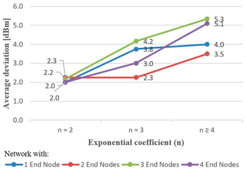
Figure 8 presents the average values of the calculated deviation between the range of the real and simulated RSSI values in a network with 1, 2, 3 and 4 end devices for different values of “n”. From the presented results, it can be concluded that the smallest deviation between the range of the real and simulated RSSI values is observed when the simulated network is configured to work with an exponential coefficient n ≈ 2. This is because this value of “n” simulates the presence of the least noise impacts in the air caused by the presence of obstacles and other sources of signals that can make the air noisy. This in turn shows that the developed simulation product is relatively reliable and suitable for studying RSSI in a Z-Wave network, as it provides an average deviation from the real results in the range of 2 dBm to 2.3 dBm. Also, the simulator results obtained at n ≈ 3 and n ≥ 4 show that the developed simulator would provide an appropriate simulation even when simulating an environment saturated with noise impacts.

6. Conclusions

This study investigates the RSSI values derived from a simulation environment in conjunction with measurements taken from an actual Z-Wave sensor network.

The experimental studies conducted show that the simulator presents results that follow the trend of deterioration of RSSI values with increasing distance between the central hub and the end devices. Experiments in a real environment confirm this trend but also show that in some cases the RSSI values remain constant regardless of the distance between the central device and the end devices. The presented average deviation with a value in the range of 2 dBm to 2.3 dBm between the results simulated with n ≈ 2 shows that the simulator presents results very close to the measured ones in the real environment. This shows that the developed simulator is suitable for studying RSSI values in a Z-Wave network. These results highlight the efficacy of the developed RSSI analysis module in modeling Z-Wave networks. For future implementation, experimental studies can be performed to prove the correctness of the simulator when examining RSSI values in a Z-Wave network saturated with interference sources.