A Machine-Learning-Based Energy Management Tool for Real-Time Integration of Distributed Energy Resources and Flexible Port Operations ^†

Abstract

Port decarbonisation requires integrated energy solutions capable of reducing fossil-fuel dependence while maintaining safety, reliability, and operational continuity. This paper presents a machine-learning-based energy management tool designed to aggregate and disaggregate energy loads according to port operational activities. The tool—modular and designed for phased deployment—integrates onshore power supply (OPS), photovoltaics (PV), vertical-axis wind turbines (VAWTs) and battery energy storage (BESS), and forecasts energy demand under different cargo-handling scenarios. It is applied to the Port of Klaipėda (Lithuania) through four capacity configurations, from a 2024 baseline (S0) to a 2035 low-carbon configuration (S3), each calibrated with real port data and evaluated under a common 2025 operational year so that the technology portfolio is isolated from inter-annual variability. Relative to the baseline, the 2035 configuration raises the renewable fraction from 0.6% to 19.4%, drops annual energy cost by 22.2% (from €8441k to €6571k) and CO₂ emissions by 18.4% (from 9679 to 7899 tCO₂/yr), and increases OPS utilisation from 0.4% to 10.6%. Random Forest demand forecasting achieves an MAE of 600.6 kW (MAPE 8.1%), improving on a persistence baseline by 25.7%, although its low R² keeps the forecasting layer to planning support rather than validated real-time control. The results establish the tool’s viability as a strategic platform for port energy transition, providing integration criteria and a scalable roadmap towards net-zero operations.

1. Introduction

Ports are critical nodes of global trade and, at the same time, significant sources of greenhouse gas emissions. The International Maritime Organization (IMO) estimates that shipping accounts for 2.89% of global CO₂ emissions [1], and a significant fraction is generated during port stays when vessels run auxiliary engines and boilers to meet on-board electrical and thermal demand. Regulation AFIR (EU) 2023/1804, which sets binding EU-wide targets for the deployment of alternative fuels infrastructure to support zero-emission mobility across all transport modes, and the FuelEU Maritime Regulation [2] impose progressively required onshore power supply (OPS) horizons to reduce these port-side emissions. In this context, port energy management systems (EMS) gain special relevance as planning and optimisation tools [3]. However, the literature shows gaps in: i. demand models traceable to published scientific sources, ii. simultaneous integration of multiple energy vectors, and iii. quantitative validation of synthetic data against real port statistics [4,5].

Existing approaches to port energy management fall into three broad families. The first includes port-scale energy audits and strategic assessment methodologies, which quantify aggregated consumption and emissions and support investment screening, but do not resolve operations at hourly or event level [3,5]. The second covers optimisation-based microgrid dispatch, typically formulated as linear or mixed-integer programmes solved over a rolling horizon and supported on generic microgrids rather than on port-specific load structures [6,7,8]. The third contains digital-twin and discrete-event simulation platforms for terminal operations, which reproduce cargo-handling logistics in detail but usually handle electricity as an exogenous cost rather than as a dispatchable resource [4]. Each family therefore settles one layer well and abstracts the other two. The present work instead couples the three layers in a single framework: a synthetic traffic generator feeds a load-disaggregation model in which every demand coefficient is traceable to a published source, and the resulting hourly series is both dispatched by a multi-criteria linear programme and used to compare machine learning forecasters. This should be read as a trade-off between early-stage applicability and operational fidelity, aimed at ports where granular AIS and terminal data are not yet available.

This paper proposes a machine-learning (ML)-based energy management tool for the integration of distributed energy resources (DER) in port operations. It is applied to the Port of Klaipėda (Lithuania) through four target infrastructure configurations: the baseline S0, associated with the 2024 starting point; the intermediate S1 and S2 configurations, associated with the 2027 and 2030 planning milestones; and the low-carbon S3 configuration, associated with 2035 (Table 1). The year attached to each scenario is a planning label for its capacity configuration, not an independent simulation year: to isolate the effect of the technology portfolio from inter-annual variability, all four configurations are evaluated over the same 2025 operational year.

Table 1. Capacity and market parameters of the four target configurations.

Parameter	S0 (2024)	S1 (2027)	S2 (2030)	S3 (2035)
PV installed [kWp]	500	2000	8000	15,000
BESS capacity [kWh]	0	2000	6000	15,000
VAWT [units × kW]	-	-	1 × 500	3 × 500
OPS berths	1	5	10	15
Grid price [€/MWh]	115	108	98	82
Emission factor [tCO2/MWh]	0.160	0.140	0.115	0.070
CO2 price [€/tCO2]	65	75	90	120

2. Materials and Methods

2.1. Tool Architecture

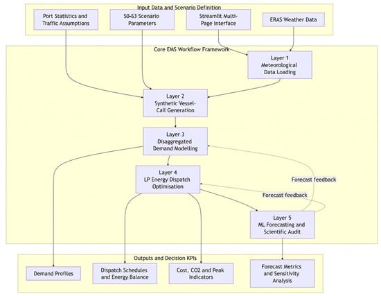
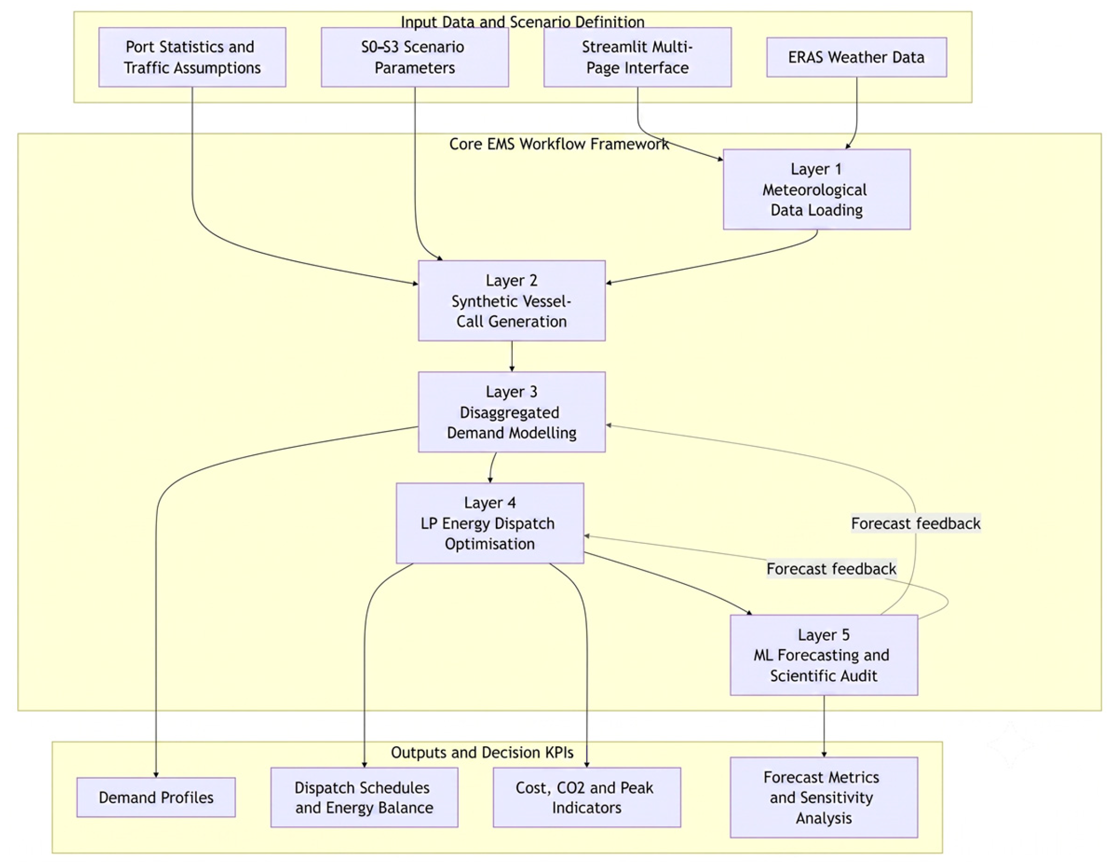
The tool is implemented in Python 3.13 with a Python Streamlit interface and a multi-page frontend application and is structured in five layers: 1. meteorological data loading (ERA5 reanalysis [9]); 2. synthetic vessel-call generation; 3. disaggregated demand modelling; 4. energy dispatch optimisation; and 5. ML-based demand forecasting. The full tool architecture and workflow are shown in Figure 1.

Figure 1. EMS tool architecture and workflow implemented in this study.

The five layers are exposed as independently switchable modules organised in three deployment phases. Phase 1 includes synthetic activity generation, load aggregation and disaggregation, asset simulation and KPI computation; phase 2 contains demand forecasting, day-ahead dispatch optimisation and sensitivity analysis; phase 3 includes intraday re-dispatch, real-time supervisory control, hydrogen dispatch and wave energy conversion. The results reported in this paper are produced with the phase 1 and phase 2 modules; the phase 3 modules are declared in the tool configuration but are not implemented in the present version. The term real-time in the title and throughout this paper refers to the temporal resolution and the receding-horizon readiness of the integration architecture, not to closed-loop supervisory control: the tool determines the coupling between port operations and distributed energy resources at hourly resolution over a full operational year rather than through annual aggregates, and the dispatch problem is formulated over an arbitrary horizon length and parameterised by the initial state of charge, so that the same linear programme can be re-solved on a moving window, applying only the first control action, without modification. Bidirectional integration with port SCADA, the battery power-conversion system and the terminal operating system is outside the scope of this work.

2.2. Synthetic Vessel-Call Generation

Vessel calls are generated using a non-homogeneous Poisson process calibrated with real port statistics and temporal patterns from Baltic maritime traffic, consistent with the Automatic Identification System (AIS)-based approach of Ship Traffic Emissions Assessment Model (STEAM [10] and STEAM2 [11]). The daily arrival rate follows:

λ(month) = λ₀ × μ_sta(month)

(1)

where λ₀ is the baseline daily arrival rate and μ_sta is a seasonal multiplier representing intra-annual Baltic traffic variation. The 2023 annual report records 5346 vessel calls [12], corresponding to an average of 14.65 calls/day; the generator used a conservative integer baseline of λ₀ = 14 calls/day, and this simplification is treated as a limitation. For each generated call, i. vessel type is sampled from the traffic mix calibrated for Klaipėda Port; ii. size class follows the Fourth IMO GHG Study 2020 [1]; and iii. stay duration uses a truncated distribution parametrised from operational phases. Coherence is verified by a systematic evaluation using five metrics (annual port call error, traffic mix MAE, seasonal consistency, OPS adoption rates, and anomalous port stays) scored on a scale of 0–100.

2.3. Vessel Berth Power Model

Berthed vessel energy demand is estimated from the Fourth IMO GHG Study 2020 methodology [1], assigning required power for auxiliary engines and boilers by vessel type, size class, and operating mode. Total berthed vessel power in kW is calculated as:

P _berth,i(t) = P_AE,i(s,m) + P_BO,i(s,m) + P_reefers,i(t)

(2)

where P_AE,i(s,m) is auxiliary engine power, P_BO,i(s,m) is boiler power (from the Fourth IMO GHG Study 2020 tables for vessel class s and mode m = at berth) [1], and P_reefers,i(t) is the additional reefer container load modelled following STEAM2 [11].

2.4. Crane and Cargo-Handling Load Model

Cargo-handling demand is modelled with two complementary methods according to vessel type. Container calls use an energy-per-move method, with electric ship-to-shore (STS) cranes assigned 11.0 kWh/move, electric rubber-tyred gantry cranes (RTGs) 7.5 kWh/move and electric reach stackers 4.0 kWh/move, as measured at a Mediterranean container terminal [13]; the electrification of RTG fleets is the single largest lever on terminal energy performance reported in the literature [14]. Moves are distributed at 65%, 30% and 5% across the three equipment types, and each container call is assigned 900 TEU at 2.0 moves per TEU. Non-container calls use an energy-per-tonne method, with coefficients ranging from 0.3 kWh/t for ferries to 5.0 kWh/t for general cargo, applied to the cargo tonnage estimated from vessel size and a vessel-type load factor; the complete coefficient table and its sources are documented in the associated source code. In both cases the resulting energy is distributed uniformly over the berth hours of each call, and all cargo-handling demand is treated as electrical.

2.5. Reefer Container and Building Load Models

Reefer container load is modelled with a nominal average power of 4 kW per reefer plug [15], with a simplified thermal correction factor based on the ideal Carnot refrigerator COP dependence. Building and HVAC thermal demand is approximated using the accumulated temperature difference method of ISO 15927-6 [16]:

HDH(t) = max(0, 18 − T_amb(t))

(3)

CDH(t) = max(0, T_amb(t) − 22)

(4)

where HDH denotes Heating Degree Hours and CDH denotes Cooling Degree Hours measured on Celsius Degrees.

2.6. LP Energy Dispatch Optimisation

Energy asset dispatch (grid, PV, VAWT, and BESS) is formulated as a linear programming problem with a rolling horizon. The multi-criteria objective function simultaneously minimises electricity purchase cost, CO₂ emission cost, and peak import penalty:

min Σ_t [w_c × E_grid(t) × π(t) + w_e × E_grid(t) × EF(t) × π_CO₂ + w_p × λ × P_peak]

(5)

where $E_{grid}\left(t\right)$ is the electricity imported from the grid at time step $t$, $\pi \left(t\right)$ is the time-varying electricity tariff, $EF\left(t\right)$ is the grid emission factor, and ${\pi }_{C{O}_2}$ is the monetised carbon price. The coefficients $w_c$, $w_e$, and $w_p$ are weighting factors for electricity cost, emission cost, and peak-shaving priority, respectively. $P_{peak}$ denotes the maximum grid import over the optimisation horizon, while $\lambda$is the penalty coefficient associated with peak demand. Constraints include hourly energy balance, battery state-of-charge dynamics, storage operational limits, and window continuity, following approaches reported in the literature [6,7,8].

The objective is solved on a 24 h rolling limit at hourly resolution, with continuity of the battery state of charge enforced between consecutive windows. The cost, emission and peak terms are all expressed in euros and normalised over the horizon, so the increment factors act directly on commensurable monetary magnitudes, and no unit scaling is required. The weights are scenario-dependent, reflecting the progressive shift in regulatory emphasis from operating cost towards emissions: ($w_c$, $w_e$, $w_p$) = (0.55, 0.30, 0.15) in S0, (0.50, 0.35, 0.15) in S1, (0.40, 0.45, 0.15) in S2 and (0.30, 0.55, 0.15) in S3, with peak-demand penalty coefficients λ of 7, 8, 10 and 12 €/kW respectively. The linear programme is built with Python Library PuLP and solved with the bundled CBC (COIN-OR Branch and Cut) solver; it is deterministic for a given input series, so repeated runs on identical inputs return identical dispatch schedules.

2.7. Demand Forecasting and Scientific Audit

Demand forecasting compares four models via a chronological 80/20 backtest: Random Forest (RF) [17], LightGBM [18], persistence, and seasonal naïve [19]. The first 80% of the hourly series is used for training and the final 20% for testing, preserving temporal order so that no future information reaches the model during training time. Predictors comprise calendar variables (hour of day, day of week, month, day of year and a weekend indicator), demand lags of 24, 48 and 168 h, 24 h and 168 h rolling means, and a temperature signal. Random Forest uses 200 trees with a maximum depth of 12, preceded by feature standardisation; LightGBM uses 300 improving rounds with a learning rate of 0.05 and 63 leaves. Both are initialised with a fixed random seed of 42. The synthetic vessel-call generator is seeded independently as 42 + (year mod 100), which yields seed 67 for the 2025 operational year; when the traffic audit does not reach the acceptance threshold, the generator scans adjacent seeds until it does, and the seed actually used is recorded with each run. The P10/P50/P90 band is constructed around the Random Forest point forecast as ±1.28 times a 168 h rolling standard deviation of the residuals; it is a residual-based interval rather than the output of a calibrated probabilistic learner and is interpreted accordingly in Section 3.3. Five metrics are used to validate the synthetic traffic: relative error in annual call counts, traffic-mix MAE, seasonal coherence, OPS rate by vessel type, and anomalous stay fraction.

3. Results

3.1. Disaggregated Demand Profile

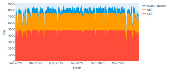
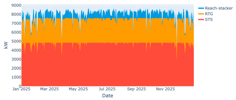
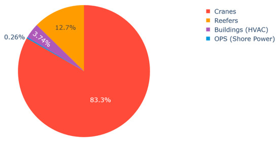
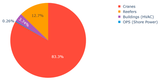
The reference scenario S0 reproduces an annual electrical consumption of 84,638 MWh, calibrated against empirical traffic statistics reported in the KVJU Annual Report 2023 [12]. Subsystem disaggregation reveals that cranes (STS/RTG/RS) constitute the dominant load at 70,481 MWh (83.3% of total), followed by reefer containers at 10,752 MWh (12.7%) and HVAC buildings at 3162 MWh (3.7%). OPS electrical demand is negligible in S0—243 MWh (0.3%)—a consequence of the 0.4% OPS connection rate in this baseline scenario. Demand shows pronounced seasonal variation, with winter peaks driven by heating and higher ferry activity (see Figure 2 and Figure 3).

Figure 2. S0 subsystem demand stacked.

Figure 3. S0 subsystem energy distribution.

3.2. Renewable Generation and Energy Balance

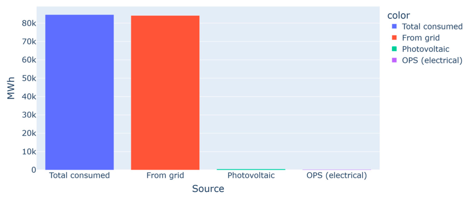
Table 2 summarises the key performance indicators for all four configurations. The renewable fraction grows from 0.6% in S0 to 19.4% in S3, driven by 15 MWp of PV combined with three 500 kW vertical-axis wind turbines. Energy cost falls by 22.2% between S0 and S3 (from €8441 k/yr to €6571 k/yr), while grid-related CO₂ emissions decrease by 18.4% (from 9679 to 7899 tCO₂/yr). OPS utilisation grows from 0.4% to 10.6%. BESS throughput increases from 0 to 6188 MWh/yr in S3, reflecting higher renewable penetration. Because all four configurations are evaluated under a common 2025 operational year and a common grid emission factor, the reported emission reduction reflects the displacement of grid imports by on-site renewables rather than any decarbonisation of the Lithuanian grid itself and is therefore a conservative lower bound on what the 2035 configuration would deliver on a 2035 grid (Figure 4).

Table 2. Main KPIs by scenario, evaluated over a common 2025 operational year.

KPI	S0	S1	S2	S3
Total consumption [MWh/yr]	84,638	84,717	84,869	85,251
Grid energy [MWh/yr]	84,165	82,824	76,502	68,689
PV energy used [MWh/yr]	473	1893	7571	14,173
VAWT energy [MWh/yr]	0	0	797	2390
BESS throughput [MWh/yr]	0	826	2440	6188
Renewable fraction [%]	0.6	2.2	9.9	19.4
Energy cost [k€/yr]	8441	8268	7533	6571
CO2 emissions [tCO2/yr]	9679	9525	8798	7899
OPS utilisation [%]	0.4	2.8	5.7	10.6
Peak demand [kW]	15,191	22,053	30,338	23,424
Average demand [kW]	9662	9672	9689	9733

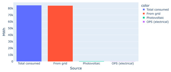
Figure 4. Annual energy balance for the baseline S0 configuration.

The peak-demand row of Table 2 is the maximum hourly value of the gross port demand series, computed before dispatch, and is therefore unaffected by BESS operation or by the peak-shaving term of the objective function. Peaks rise from S0 to S2 as the growing number of OPS berths transfers vessel auxiliary load onto the shore supply. The lower value in S3 does not reverse that trend: each configuration is evaluated on its own synthetic vessel-call realisation, whose seed is selected by the traffic auto-calibration routine, so the annual maximum is a single extreme order statistic of that realisation. The four configurations differ by less than 1% in annual consumption (84,638 to 85,251 MWh), which limits the combined effect of OPS load transfer and realisation noise on the annual aggregates, whereas the cost and emission differences attributed to the technology portfolio are of the order of 18% to 22%. The comparison in Table 2 is therefore unaffected; only the annual maximum, as a single extreme order statistic, is materially realisation-sensitive, and the peak row should be read as indicative of the order of magnitude rather than as a KPI directly comparable across configurations.

3.3. Demand Forecasting

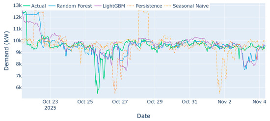
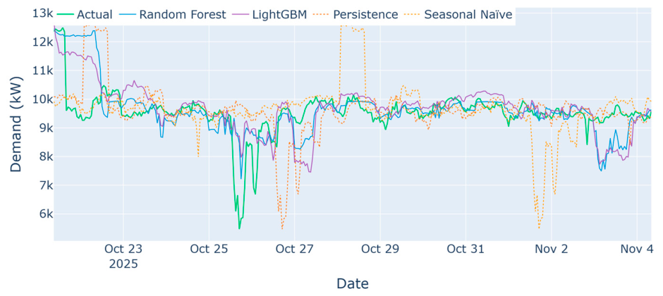
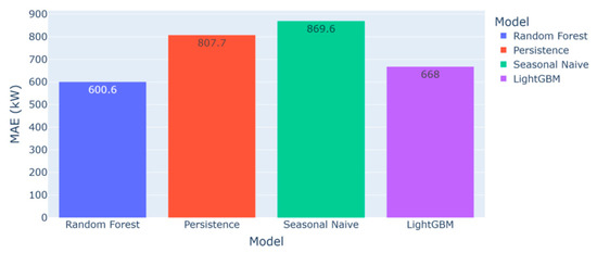
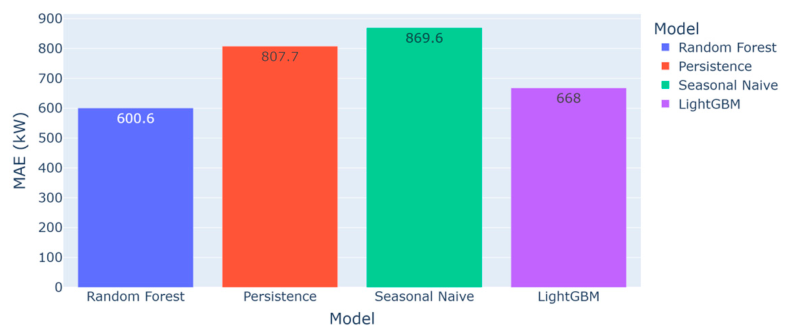
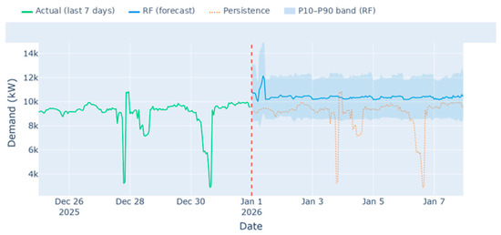
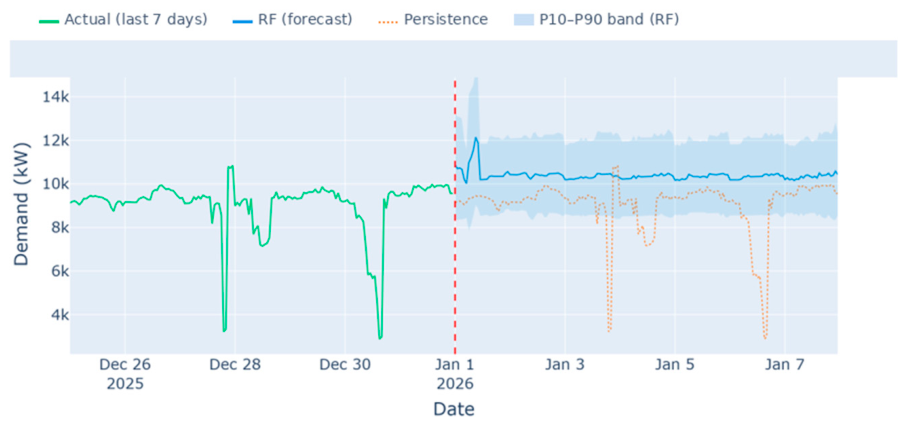
In Table 3, the Random Forest model achieves the lowest MAE at 600.6 kW compared to 807.7 kW for the persistence model, a 25.7% improvement; LightGBM reaches 668.0 kW. The coefficient of determination is nonetheless low for all models (R² = 0.167 for RF and 0.124 for LightGBM), and this deserves explicit comment. Hourly port demand is dominated by discrete, quasi-random cargo-handling events—individual crane cycles and vessel arrivals—whose timing is not recoverable from calendar variables or from recent demand history. The structure that the models can learn therefore accounts for only a small share of total variance. That this variance is basically hard rather than simply unmodelled is indicated by the strongly negative R² of the persistence and seasonal naïve baselines (−0.698 and −0.780), which perform worse than predicting the sample mean. Random Forest should therefore be read as the best baseline among those tested rather than as a strong predictor: an MAE of 600.6 kW is 6.2% of mean demand, which supports day-ahead comparison and planning, but not validated real-time control. The P10-P90 band, constructed from the rolling standard deviation of the residuals rather than by a calibrated probabilistic model, covers 86.6% of observations with a mean width of 2311 kW over a 336 h evaluation window and 84.5% with a mean width of 2338 kW when recomputed over the complete 1719 h test set. A P10-P90 interval is nominally an 80% central interval, so the band is slightly conservative; narrowing it, and calibrating it properly, would require the event-level information discussed in Section 4 (Figure 5, Figure 6 and Figure 7).

Table 3. Forecasting model comparison for scenario S0 with 80/20 backtest.

Model	MAE [kW]	RMSE [kW]	MAPE [%]	R2
Random Forest (RF)	600.6	1018.6	8.1	0.167
LightGBM	668.0	1044.3	8.8	0.124
Persistence	807.7	1454.2	10.6	−0.698
Seasonal Naïve	869.6	1489.3	11.5	−0.780

Figure 5. S0 forecasting validation—actual vs. Random Forest.

Figure 6. Model MAE comparison.

Figure 7. Seven-day forward forecast with P10-P90 probabilistic bands.

3.4. Sensitivity Analysis

The one-at-a-time (OAT) sensitivity values in Table 4 are post-processing perturbations of the reported S0 annual aggregates rather than full re-optimisations of the dispatch problem. Each input is varied by ±20% and the affected cost or emission term is recomputed analytically. A 20% increase in the grid electricity price raises the reported cost by €1,688,283, which is by construction 20% of the baseline energy cost of €8441k. The carbon-price and grid-emission-factor perturbations yield the same cost change of €154,862 because both are monetised through the same product of emissions and an auxiliary carbon price of €80/tCO₂; they differ in their physical effect, since only the emission factor changes emissions, by 1936 tCO₂ (20.0%). PV capacity has very limited cost impact in S0 (+€9494; <0.2%) given the minimal solar installation (500 kWp). These results indicate the relative leverage of each parameter on the reported aggregates: grid electricity price dominates cost, and the grid emission factor governs emissions. They should not be interpreted as dispatch responses, since the optimiser was not re-run for each perturbation. Values are post-processing perturbations of the S0 annual aggregates, not full re-optimisations. Carbon price and grid emission factor share the same ΔCost because both are monetised through the same emissions × carbon-price product; the carbon price does not affect physical emissions, hence the null ΔCO₂ entry.

Table 4. OAT sensitivity analysis results (±20%, S0).

Parameter	ΔCost (+20%)	ΔCO2 (+20%)
Grid price	+€1,688,283	0
Carbon price	+€154,862	0
Grid emission factor	+€154,862	+1936 tCO2
PV capacity	+€9494	−11 tCO2

4. Discussion

The results confirm that the progressive combination of OPS, PV, BESS, and VAWT can substantially reduce port emissions and costs by 2035. The renewable fraction of 19.4% in S3 is achieved by combining 15 MWp PV with 3 × 500 kW VAWTs, supported by a BESS throughput of 6188 MWh/yr that absorbs generation variability. The 22.2% cost reduction from S0 to S3 exceeds the 18.4% emission reduction, reflecting the structural grid price decline assumed across configurations. The scenarios assume lithium-ion BESS parameters. Iron-based aqueous redox-flow batteries are a relevant alternative for stationary port applications, given potentially low-cost active materials, operational safety and long cycle life [20]; however, lower energy density, pumping losses, balance-of-plant requirements, footprint and commercial maturity would have to be assessed against port constraints, so the present results should not be read as a technology-neutral battery comparison.

Study limitations include the following. The vessel-call process was checked against aggregate annual statistics, traffic mix, seasonality, OPS adoption and anomalous stays, rather than against hourly AIS arrivals, berth occupancy or event-level terminal records; this is an aggregate plausibility check and not an operational validation. Forecast skill was limited, with a best R² of 0.167, and the reported uncertainty band is residual-based rather than produced by a calibrated probabilistic learner. The dispatch evaluation assumes perfect foresight within each 24 h horizon and does not propagate forecasting errors into the operational KPIs, so the reported costs and emissions should be read as an optimistic guarantee of closed-loop performance. The PV model omits shading and module degradation, and the integrated audit identifies a failure in the OPS-type MAE metric, indicating that OPS adoption by vessel type requires further calibration. These limitations restrict the conclusions to comparative planning analysis and do not show real-time operational performance. Future research will include real-time AIS data integration, refinement of OPS adoption curves by vessel type, and extension of the optimiser to stochastic programming or model predictive control. Of these, closing the loop is the immediate step: re-optimising the 24 h dispatch problem at each hourly step using updated forecasts and the current state of charge and applying only the first control action before moving the horizon forward. This requires no change to the optimisation formulation, but it does require the forecast error characterised in Section 3.3 to be propagated into the dispatch decisions; until that evaluation is performed, the costs and emissions of Table 2 are the open-loop bound against which a receding-horizon implementation would be compared. Hydrogen-fuelled terminal tractors, considered during the design of the tool but not modelled in the present version, are a further planned extension: their inclusion would turn the dispatch problem into a multi-vector electricity-hydrogen coupling problem, for which fleet-level energy management strategies accounting for fuel-cell state-of-health disparity [21] and flexible on-grid and off-grid control of electricity-hydrogen microgrids [22] offer relevant recent methodological references.

5. Conclusions

A modular port energy management tool has been presented and applied to the Port of Klaipėda across four target infrastructure configurations (S0-S3), associated with the 2024, 2027, 2030 and 2035 planning milestones and all evaluated over a common 2025 operational year. The main findings are:

• Electrical disaggregation into four subsystems reveals that cranes dominate port demand (83.3% in S0), while OPS electrical demand is negligible in the baseline (0.4%) and grows to 10.6% in S3 as the connection rate increases.
• Scenario S3 (2035) achieves a 19.4% renewable fraction and a 18.4% CO₂ reduction from S0, with energy cost reduced by 22.2%, subject to full implementation of AFIR and FuelEU Maritime.
• Random Forest is the best forecasting baseline tested in S0 (MAE = 600.6 kW; MAPE = 8.1%), outperforming persistence by 25.7% in MAE, although its low R² (0.167) indicates that most demand variance remains unexplained and confines the forecasting layer to planning support rather than validated real-time control.
• Sensitivity analysis shows that grid price is the main cost driver (elasticity ≈ 1.0), while the emission factor governs emissions with the same elasticity.
• The integrated scientific audit (82.0/100) validates synthetic traffic coherence in four of five metrics, with OPS-type behaviour as the only failure pending correction in future iterations.

References

- IMO. Fourth IMO GHG Study 2020-Full Report and Annexes. Available online: https://n9.cl/mxmdw (accessed on 15 January 2026).
- Regulation (EU) 2023/1804 of the European Parliament and of the Council of 13 September 2023 on the Deployment of Alternative Fuels Infrastructure, and Repealing Directive 2014/94/EU. Available online: https://n9.cl/1qzg3 (accessed on 15 January 2026).
- Montuori, L.; Alcázar-Ortega, M.; Díaz-Bello, D.; Vargas-Salgado, C. Towards the decarbonization of the maritime industry: Design of a novel methodology for the sustainable strategy assessment. Sustain. Energy Technol. Assess. 2025, 83, 104632. [Google Scholar] [CrossRef] [Scilit]
- Carlan, V.; Sys, C.; Vanelslander, T.; Roumboutsos, A. Digital innovation in the port sector: Barriers and facilitators. Compet. Regul. Netw. Ind. 2017, 18, 71–93. [Google Scholar] [CrossRef] [Scilit]
- Acciaro, M.; Vanelslander, T.; Sys, C.; Ferrari, C.; Roumboutsos, A.; Giuliano, G.; Lam, J.S.L.; Kapros, S. Environmental sustainability in seaports: A framework for successful innovation. Marit. Policy Manag. 2014, 41, 480–500. [Google Scholar] [CrossRef] [Scilit]
- Palma-Behnke, R.; Benavides, C.; Lanas, F.; Severino, B.; Reyes, L.; Llanos, J.; Sáez, D. A Microgrid Energy Management System Based on the Rolling Horizon Strategy. IEEE Trans. Smart Grid 2013, 4, 996–1006. [Google Scholar] [CrossRef] [Scilit]
- Parisio, A.; Rikos, E.; Glielmo, L. A Model Predictive Control Approach to Microgrid Operation Optimization. IEEE Trans. Control Syst. Technol. 2014, 22, 1813–1827. [Google Scholar] [CrossRef] [Scilit]
- Georgiou, G.S.; Christodoulides, P.; Kalogirou, S.A. Optimizing the energy storage schedule of a battery in a PV grid-connected nZEB using linear programming. Energy 2020, 208, 118177. [Google Scholar] [CrossRef] [Scilit]
- Hersbach, H.; Bell, B.; Berrisford, P.; Hirahara, S.; Horányi, A.; Muñoz-Sabater, J.; Nicolas, J.; Peubey, C.; Radu, R.; Schepers, D.; et al. The ERA5 global reanalysis. Q. J. R. Meteorol. Soc. 2020, 146, 1999–2049. [Google Scholar] [CrossRef] [Scilit]
- European Environment Agency. EMEP/EEA Air Pollutant Emission Inventory Guidebook 2019: Technical Guidance to Prepare National Emission Inventories; Publications Office: Luxembourg, 2019. [Google Scholar] [CrossRef]
- Jalkanen, J.P.; Johansson, L.; Kukkonen, J.; Brink, A.; Kalli, J.; Stipa, T. Extension of an assessment model of ship traffic exhaust emissions for particulate matter and carbon monoxide. Atmos. Chem. Phys. 2012, 12, 2641–2659. [Google Scholar] [CrossRef] [Scilit]
- Klaipeda Annual Report. 2023. Available online: https://n9.cl/2hi69 (accessed on 15 April 2026).
- Martínez-Moya, J.; Vazquez-Paja, B.; Gimenez Maldonado, J.A. Energy efficiency and CO2 emissions of port container terminal equipment: Evidence from the Port of Valencia. Energy Policy 2019, 131, 312–319. [Google Scholar] [CrossRef] [Scilit]
- Yang, Y.C.; Chang, W.M. Impacts of electric rubber-tired gantries on green port performance. Res. Transp. Bus. Manag. 2013, 8, 67–76. [Google Scholar] [CrossRef] [Scilit]
- Acciaro, M.; Ghiara, H.; Cusano, M.I. Energy management in seaports: A new role for port authorities. Energy Policy 2014, 71, 4–12. [Google Scholar] [CrossRef] [Scilit]
- ISO 15927-6:2007; Hygrothermal Performance of Buildings-Calculation and Presentation of Climatic Data-Part 6: Accumulated Temperature Differences (Degree-Days). International Organization for Standardization: Geneva, Switzerland, 2007.
- Breiman, L. Random Forests. Mach. Learn. 2001, 45, 5–32. [Google Scholar] [CrossRef] [Scilit]
- Ke, G.; Meng, Q.; Finley, T.; Wang, T.; Chen, W.; Ma, W.; Ye, Q.; Liu, T. LightGBM: A Highly Efficient Gradient Boosting Decision Tree. In Proceedings of the 31st Conference on Neural Information Processing Systems, Long Beach, CA, USA, 4–9 December 2017; pp. 3149–3157. [Google Scholar]
- Hyndman, R.J.; Koehler, A.B. Another look at measures of forecast accuracy. Int. J. Forecast. 2006, 22, 679–688. [Google Scholar] [CrossRef] [Scilit]
- Zhang, H.; Sun, C. Cost-effective iron-based aqueous redox flow batteries for large-scale energy storage application: A review. J. Power Sources 2021, 493, 229445. [Google Scholar] [CrossRef] [Scilit]
- Mei, J.; Li, Z.; Song, K.; Meng, X.; Wu, H.; Tang, X.; Hasanien, H.M.; Li, Y.; Sun, C. SOH-disparity-aware energy management for multi-stack fuel cells using enhanced soft actor-critic reinforcement learning. IEEE Trans. Transp. Electrif. 2026, early access. [Google Scholar] [CrossRef] [Scilit]
- Wang, Z.; Fan, F.; Zhang, H.; Song, K.; Jiang, J.; Sun, C.; Xue, R.; Zhang, J.; Chen, Z. Flexible on-grid and off-grid control for electric-hydrogen coupling microgrids. Energies 2025, 18, 985. [Google Scholar] [CrossRef] [Scilit]
Disclaimer/Publisher’s Note: The statements, opinions and data contained in all publications are solely those of the individual author(s) and contributor(s) and not of MDPI and/or the editor(s). MDPI and/or the editor(s) disclaim responsibility for any injury to people or property resulting from any ideas, methods, instructions or products referred to in the content. |
© 2026 by the authors. Licensee MDPI, Basel, Switzerland. This article is an open access article distributed under the terms and conditions of the Creative Commons Attribution (CC BY) license.