


Abstract
The increasing use of robotic manipulators in construction requires precise trajectory planning to reduce oscillations, dynamic loads, and positioning errors. Trajectory planning, understood as determining the manipulator’s motion from an initial to a final configuration while satisfying specified kinematic and dynamic constraints, is a fundamental part of motion planning. Polynomial trajectories are widely applied because they ensure smoothness and allow specifying boundary conditions on velocity and acceleration. However, higher-degree polynomials introduce computational complexity. This study develops the analytical framework for seventh-degree polynomial trajectory generation for horizontal motion with smooth acceleration and deceleration, achieving prescribed maximum velocity and acceleration and identifying the conditions for including a uniform-motion segment.
1. Introduction
In recent decades, robotic technologies have been intensively implemented in construction. Numerous theoretical and experimental studies have been conducted by various researchers, resulting in the development of diverse concepts for automation and robotization of construction processes [1]. The increased degree of mechanization and automation in construction processes has led to the complexity of activities related to the design, adjustment, programming, and maintenance of equipment. Problems have arisen related to the difficulties in adapting to the working conditions of construction sites and the need to develop large-scale robotic machines while maintaining high accuracy in the operations performed [2]. This necessitates the definition and solution of fundamental research tasks that allow the synthesis of advanced designs for the construction of robotic manipulators with predetermined characteristics. One such fundamental task is to plan the movement of machines or their units to minimize dynamic structural loads and vibrations. Numerical studies in [3,4,5,6] showed that, by using laws with smooth increases and decreases in displacement, the dynamic behavior of machines can be significantly improved. Polynomials of a high degree are particularly suitable for motion planning, because they provide smoothness and allow the kinematic characteristics of the motion to be specified both at the beginning and the end of the motion [7,8,9,10], but the calculation of additional coefficients is complex.
2. Problem Statement
In works [11,12] a mathematical model of a robotic construction manipulator with a Cartesian kinematic structure, a freely suspended load, and a fixed load were developed. The manipulator performs three types of rectilinear motions: longitudinal horizontal motion, transverse horizontal motion of the working tool, and vertical motion of the working tool. We considered the longitudinal horizontal motion of the manipulator because the largest displacements that occur during transportation operations are in this direction and involve high velocities and accelerations. This, combined with the considerable height of the manipulator and elasticity of its metal structure, results in significant oscillations. The effects of increasing machine speeds and accelerations are most pronounced during transitional phases such as startup and stopping. The primary effect is the excitation of vibrations in the structure, which can be mitigated by controlling the drive motor according to a law that ensures smooth starting and stopping. The motion law should satisfy various criteria [9], with particular importance placed on implementing a motion law that provides specified values of kinematic characteristics, such as velocity and acceleration, to enhance the functionality of the machine. In [13], an algorithm for trajectory planning based on a fifth-degree polynomial law with an intermediate segment of uniform motion was developed. A comparison was made between the two motion laws, where it was found that in a motion law with a uniform section, the duration of motion was shorter, and the preassigned maximum values of the speed and acceleration were achieved. The angle of oscillation of the vertical column is very small owing to the smooth acceleration and stopping. If a seventh-degree polynomial law is used for motion planning, which allows the inclusion of the derivative of acceleration, even smoother motion is ensured and the dynamic response of the machine is improved [11,13].
In the present work, the analytical foundations of manipulator trajectory planning according to a seventh-degree polynomial law are provided, which will provide an even smoother change in displacement. We set ourselves the goal of finding seventh-degree polynomials of that describe the movement in stages of acceleration and stopping as well as determining the conditions under which a section with uniform motion can be included.
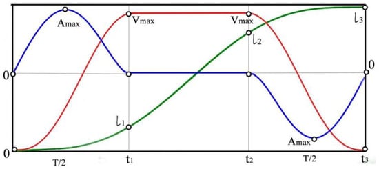
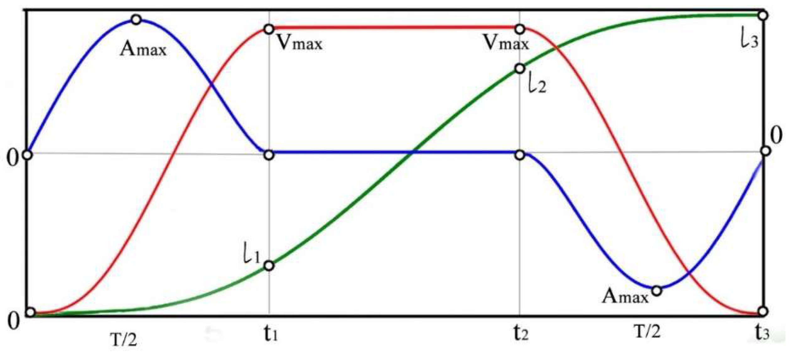
The displacement performed by the machine is represented by the diagram in Figure 1. To achieve the maximum performance of the machine, it is necessary to perform as much movement as possible at the maximum permissible speed, i.e., to include a section with uniform motion in the speed diagram. Half of the parameter is used to accelerate to the preassigned speed during the interval from 0 to , followed by a period of uniform motion during the time interval from to . The other half of the parameter is used to decelerate from the maximum speed to zero during the interval from to , where is the duration of the motion. The durations of the acceleration and deceleration periods are equal to .
Figure 1.
A trajectory with an intermediate section with uniform motion.
3. Main Statements and Proofs
3.1. Statement 1
In the set of all seventh-degree polynomials, , there exists only one satisfying the following conditions:
where and .
This polynomial is
and its derivatives up to the third order are
Proof.
Imposing the conditions (1) we obtain and therefore
Imposing conditions (2) we obtain the system
which has only one solution: .
We substitute the coefficients into the expression for and get
from where by differentiation, we obtain the final form of and . □
3.2. Statement 2
Let and be the functions obtained in Statement 1. In such a case,
- is a strictly increasing function on the interval
- in the interval and
- in the interval , in the interval ,where .
Proof.
From the expression (6) for follows
where and are the roots of the polynomial . □
Thus we obtain that the function is strictly monotonically increasing in the intervals and , and strictly monotonically decreasing in the interval ; therefore
From the expression (5) for follows
and so, it follows that the function is strictly monotonically increasing in the interval and strictly monotonically decreasing in the interval ; therefore
From the expression (4) for follows and so we obtain that is a strictly monotonically increasing function in the interval .
As a direct consequence of (8) and (9), the following dependencies are obtained:
4. Obtained Results
The analysis of the obtained results indicates that three trajectory variants are possible depending on the values of the preset displacement and the calculated parameter —a limit displacement, in which the set maximum values of speed and acceleration can be simultaneously achieved.
When the preset displacement is smaller than the limit displacement, it is not possible to concurrently achieve the pre-assigned values of the maximum velocity and acceleration. In most cases, the maximum acceleration is the determining factor for the kinematic characteristics of motion. From (11), the maximum possible velocity that satisfies the preassigned value of the maximum acceleration is determined
In the second variant, the preset displacement is equal to the limit displacement—the trajectory is entirely polynomial (3). The preset maximum velocity and acceleration can be reached simultaneously, but a segment of uniform motion cannot be included.
We are particularly interested in the third case, in which the preset displacement is greater than the limit displacement. It is possible to synthesize a trajectory with an intermediate section of uniform motion for preassigned values of the maximum velocity and acceleration.
Let and be the functions defined by (3), (4) and (5), respectively.
Let and be predetermined maximum velocity and acceleration, respectively, and let the parameters and be chosen so that (10) and (11) are satisfied.
In the third variant we have
From (13), it follows that
By definition
From the expression (4), it immediately follows that
From (14) and (15) it follows that , i.e.,
Let the function describe the instantaneous velocity.
We define
We introduce the functions , and as follows:
where
Using (15) and (16) we obtain that
If , then by using (14), (21), (22) and (23) we have:
and therefore
We define the function in the following way:
It can be proven that is a three-times continuously differentiable function in the interval (at all points except and , this function is infinitively differentiable).
Also, we have
Thus, the function describes the displacement from the initial moment to current moment .
Let
Then, by using (15), we obtain
The function describes the instantaneous acceleration.
5. Conclusions
The developed trajectory planning algorithm, based on seventh-degree polynomials, ensures smooth transitions through the three sections of motion: acceleration, uniform motion, and deceleration. Three possible trajectory variants for planning longitudinal horizontal motion are considered, depending on the length of displacement that needs to be covered and the achievement on the preassigned maximum speed and acceleration. When the preset displacement exceeds the calculated limit, the trajectory can consist of polynomial acceleration and deceleration phases with an intermediate segment of uniform motion. The resulting polynomials can be used for trajectory planning of the longitudinal motion of machines or their elements where smooth motion and precise positioning are required.
Author Contributions
Conceptualization, M.I. and H.G.; methodology, H.G. and M.I.; formal analysis, M.I.; investigation, H.G.; writing—original draft preparation, M.I. and H.G.; writing—review and editing, M.I. and H.G.; visualization, M.I.; supervision, M.I.; project administration, M.I. All authors have read and agreed to the published version of the manuscript.
Funding
This research was supported by the Research and Development Sector at the Technical University of Sofia.
Institutional Review Board Statement
Not applicable.
Informed Consent Statement
Not applicable.
Data Availability Statement
Data are contained within the article.
Acknowledgments
The authors would like to thank the Research and Development Sector at the Technical University of Sofia for their financial support.
Conflicts of Interest
The authors declare no conflicts of interest.
References
- Saidi, K.S.; Bock, T.; Georgoulas, C. Robotics in Construction. In Springer Handbook of Robotics; Siciliano, B., Khatib, O., Eds.; Springer: Cham, Switzerland, 2016; pp. 1493–1520. [Google Scholar]
- Bulgakov, A.; Vorobyov, V. Industrial Robots. Kinematics, Dynamics, Control and Management; Solon Press: Moscow, Russia, 2012. (In Russian) [Google Scholar]
- Abe, A. An effective trajectory planning method for simultaneously suppressing residual vibration and energy consumption of flexible structures. Case Stud. Mech. Syst. Signal Process. 2016, 4, 19–27. [Google Scholar] [CrossRef] [Scilit]
- Qie, N.; Houa, W.-F.; He, J.-H. The fastest insight into the large amplitude vibration of a string. Rep. Mech. Eng. 2021, 2, 1–5. [Google Scholar] [CrossRef] [Scilit]
- Siciliano, B.; Sciavicco, L.; Villani, L.; Oriolo, G. Robotics: Modeling, Planning and Control; Springer: Berlin/Heidelberg, Germany, 2009. [Google Scholar]
- He, C.J.-H.; García, A. The simplest amplitude–period formula for non-conservative oscillators. Rep. Mech. Eng. 2021, 2, 143–148. [Google Scholar] [CrossRef] [Scilit]
- Kalinkov, S.; Mitrev, R.; Ruzhekov, G. Simulation modelling and study of elevating transfer vehicle with controlled electric motor of the travel mechanism. Mech. Mach. 2009, 82, 71–78. (In Bulgarian) [Google Scholar]
- Kalinkov, S. Research on Electronic Power Supply and Control Systems of Automated Storage and Retrieval Machines. Ph.D. Thesis, Technical University of Sofia, Sofia, Bulgaria, 2011. (In Bulgarian) [Google Scholar]
- Mitrev, R. Development of the Theory for Designing, Modelling and Research of Construction and Lifting Manipulators. Doctoral Dissertation, Technical University of Sofia, Sofia, Bulgaria, 2019; pp. 290–301. (In Bulgarian) [Google Scholar]
- Biagiotti, L.; Melchiorri, C. Trajectory Planning of Automatic Machines and Robots; Springer: Berlin/Heidelberg, Germany, 2008. [Google Scholar]
- Ivanova, M. A Study of the Longitudinal Motion of a Robotic Construction Manipulator. Ph.D. Thesis, Technical University of Sofia, Sofia, Bulgaria, 2023. (In Bulgarian) [Google Scholar]
- Panov, V.; Ivanova, M.; Mitrev, R. Mathematical modeling of the longitudinal motion of a robotic construction manipulator with a freely suspended payload. In Proceedings of the American Institute of Physics Conference Series; AIP Publishing: Melville, NY, USA, 2022; Volume 2557, p. 040003. [Google Scholar]
- Mitrev, R.; Panov, V.; Ivanova, M. Trajectory planning of a robotic construction manipulator motion based on a fifth-degree polynomial with preassigned maximum velocity and acceleration. In Proceedings of the American Institute of Physics Conference Series; AIP Publishing: Melville, NY, USA, 2022; Volume 2557, p. 040004. [Google Scholar]
Disclaimer/Publisher’s Note: The statements, opinions and data contained in all publications are solely those of the individual author(s) and contributor(s) and not of MDPI and/or the editor(s). MDPI and/or the editor(s) disclaim responsibility for any injury to people or property resulting from any ideas, methods, instructions or products referred to in the content. |
© 2026 by the authors. Licensee MDPI, Basel, Switzerland. This article is an open access article distributed under the terms and conditions of the Creative Commons Attribution (CC BY) license.