Proceeding Paper

Adversarial Robustness and Explainability in AI-Generated Face Detection †
by
Georgi Kotov
*,
Plamen Nakov
and
Ognyan Nakov
Faculty of Computer Systems and Technologies, Technical University of Sofia, 8 Kliment Ohridski Blvd, 1756 Sofia, Bulgaria
*
Author to whom correspondence should be addressed.
Presented at the 15th International Scientific Conference TechSys 2026—Engineering, Technologies and Systems, Plovdiv, Bulgaria, 14–16 May 2026.
Eng. Proc. 2026, 150(1), 52; https://doi.org/10.3390/engproc2026150052

Published: 22 July 2026

Abstract

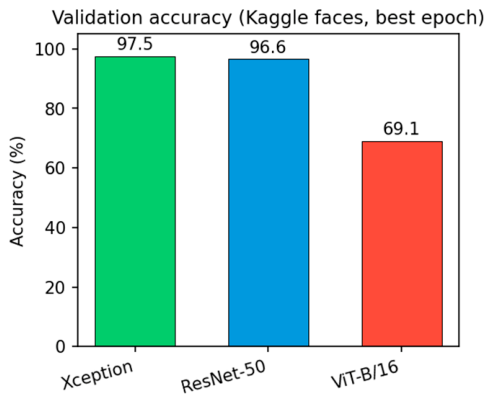
This paper investigates adversarial robustness and explainability in AI-generated face detection through the Robust and Explainable Detection (RED) framework. RED unifies CNN and Vision Transformer (ViT) backbones with FGSM/PGD adversarial training and Grad-CAM-based interpretability in one reproducible pipeline. Experiments on the Kaggle real/fake face dataset with stratified 70/15/15 splits report accuracy, F1, AUC-ROC, Adversarial Robustness Index (ARI), and Explainability Fidelity (EF). Xception and ResNet-50 reach 97.53% and 96.64% validation accuracy, respectively, while ViT-B/16 attains 69.08%. RED supports forensic and legal applications requiring both detection accuracy and transparent model behavior.

1. Introduction

Deep generative models such as Generative Adversarial Networks (GANs) [1] and diffusion models [2] can now synthesize faces with photorealistic detail, natural lighting, and convincing local texture. This progress has clear technical value, yet it also creates a practical detection problem: visual inspection alone is often insufficient to separate authentic facial images from synthetic ones, especially after resizing, recompression, or reposting across platforms.
For this reason, AI-generated face detection is no longer only a benchmark problem. It affects identity verification workflows, media authenticity checks, platform moderation, and the evidentiary value of digital images. Strong pipelines increasingly rely on residual-network designs [3] and ViT-style encoders [4] whose transformer blocks follow the self-attention formulation of Vaswani et al. [5]. Benchmarking also spans standardized face-forgery datasets [6] and large demographically annotated synthetic-face corpora [7]. Reliability nonetheless becomes much less certain when the input is slightly shifted from the conditions seen during training or when an attacker deliberately crafts perturbations that preserve human-level realism.
In this paper, adversarial robustness is treated as an empirical property of the detector: how much performance is retained when the same sample is evaluated after a constrained perturbation designed to change the model output, in line with foundational adversarial-example formulations [8]. Optimization-based robust training objectives [9] further shape what “robustness” means in practice. Early analyses of network sensitivities [10] motivate measuring brittleness rather than trusting headline accuracy alone. This framing is important for deepfake detection because a model may appear strong on clean data while relying on brittle image cues that disappear under small gradient-based modifications.
To study that problem in a targeted way, this work develops a Robust and Explainable Detection (RED) framework for still-image face classification. RED combines multi-stream feature extraction with adversarial training and post hoc explanation so that robustness and interpretability are examined within one pipeline rather than as separate add-ons.
The main contributions of this work are threefold. First, the paper defines a unified RED framework that combines CNN, ViT, and optional spectral representations for AI-generated face detection. Second, it implements a reproducible training and evaluation workflow with FGSM/PGD attacks, robustness-oriented metrics, and Grad-CAM visualization. Third, it analyzes how robustness and explanation quality interact in this application setting, while clearly separating the results reported in the current experiments from the extensions planned for future evaluation.
The study is intentionally scoped to still facial images. Video-level manipulations, temporal consistency cues, and real-time deployment constraints are outside the present experiments. The attack setting considered here is an L∞-bounded white-box scenario because it offers a controlled way to test whether the detector depends on unstable cues; broader transfer-based and black-box settings are discussed as future extensions rather than claimed as completed evaluations.
The remainder of the paper is structured as follows. Section 2 summarizes prior work most relevant to this study: deepfake detection under adversarial pressure, explainability methods for forged-face analysis, defense strategies, and metrics for explanation assessment. Section 3 presents the RED methodology. Section 4 describes training and evaluation. Section 5 discusses results and limitations.

2. Related Work

This section reviews the prior studies that directly inform the design choices in RED. Rather than attempting a broad survey of all deepfake-detection research, the discussion focuses on four points needed for this paper: how detectors fail under adversarial manipulation, how explanation methods are used in face-forgery analysis, which defensive strategies are relevant to the present implementation, and how explanation quality can be assessed when manipulation masks are available.
Research on deepfake detection now spans CNN-based detectors, transformer models, fusion architectures, and forensic pipelines that combine spatial, frequency, and compression cues. For the purposes of this paper, the most relevant gap is not the absence of high clean-data accuracy, but the limited number of studies that connect detector performance, adversarial stability, and explanation quality within one reproducible setup.

2.1. Adversarial Vulnerabilities in Deepfake Detection

Many published detectors are trained and reported under clean-image conditions, so their headline metrics mainly describe performance when the evaluation data remains close to the original benchmark distribution. For deployment-oriented use, however, that is not enough: synthetic-face detectors may be exposed to resized, compressed, reposted, or intentionally manipulated inputs, and those changes can reveal whether the model depends on fragile evidence rather than durable forensic cues.
The present implementation therefore includes both FGSM and PGD in src/attacks.py. FGSM applies a single gradient-sign step, while PGD performs multiple projected updates within the same perturbation budget. In this paper these attacks are not introduced as a generic survey topic, but as the concrete mechanisms used to probe the RED models under controlled conditions. Broader attack families include iterative boundary approximations [11] and practical black-box attacks based on transfer and substitute models [12].
Prior empirical work on deepfake detectors shows that undefended models can lose substantial accuracy even under modest L∞ perturbations, with large drops reported across several architectures, which supports the practical motivation for evaluating robustness here: strong clean performance alone does not guarantee that the detector is learning stable manipulation evidence.
Another relevant finding from the literature is that detector behavior already varies across manipulation families, compression levels, and dataset construction choices before adversarial perturbations are added. This matters for the current study because any robustness result must be interpreted together with dataset scope; a model that is resilient on one benchmark may still generalize poorly when the manipulation process or image pipeline changes.

2.2. Explainability in Deepfake Detection

Interpretability is especially important in forged-face analysis because a binary prediction by itself does not reveal whether the detector focused on a plausible artifact or on an incidental shortcut. In operational settings such as moderation support, media review, or forensic screening, users often need some visual indication of why a face was labeled as synthetic or authentic.
For face forgery detection, useful explanations should ideally align with artifact-bearing regions such as blending boundaries, local texture inconsistencies, asymmetries in facial structure, or unnatural illumination transitions. At the same time, explanation maps must be treated cautiously: a visually sharp saliency pattern does not automatically prove that the model relied on semantically meaningful evidence.
In this work, explainable AI is considered primarily as an analysis tool for model behavior rather than as a standalone research objective. Grad-CAM is emphasized because it can be applied efficiently to the CNN branch of RED and produces spatial heatmaps that are practical to compare across clean and adversarial conditions; complementary attribution tools are discussed next.
Selvaraju et al. introduced Grad-CAM [13] and demonstrated that class-specific gradients can be combined with final convolutional activations to localize influential image regions. Since then, Grad-CAM has become a common diagnostic method in computer vision and a practical choice for studies, such as this one, that need a lightweight and architecture-aware visualization of detector attention.
Layer-wise relevance propagation [14] and integrated gradients [15] provide pixel- and path-based attributions with different inductive biases. Transformer-specific interpretability beyond pure attention maps [16] is increasingly relevant when ViT backbones are used. Instance-level tools such as LIME [17] and SHAP [18] remain common baselines, and randomized input sampling (RISE [19]) supports perturbation-based saliency for black-box models.
Existing comparisons of explanation methods for deepfake detection generally suggest a trade-off between interpretability detail, computational cost, and stability. That observation motivates the use of Grad-CAM here: the method is fast enough for repeated inspection during model analysis, while still providing localized heatmaps that can be checked against visible manipulations or available masks.
Recent work has also examined how adversarial perturbations affect explanations themselves, indicating that explanation quality can degrade when the input is deliberately manipulated, which is directly relevant to RED because the framework aims to assess not only whether the label changes, but also whether the model’s visual reasoning becomes less consistent under attack.
Quantitative evaluation of explanation methods in deepfake detection is still comparatively limited. When studies compare multiple explanation methods on shared benchmarks, the conclusions are usually conditional on the dataset, the detector family, and the availability of ground-truth artifact masks. This is one reason the present paper treats explanation metrics as complementary evidence rather than as a standalone proof of model validity.
For this application, the practical question is not only where the model attended, but whether that attention remains coherent when the detector is stressed. Accordingly, the explainability discussion in this paper is tied to the trained RED models, their clean-versus-adversarial behavior, and the availability of mask-based comparison where the dataset permits it.

2.3. Adversarial Defense Strategies

The defense literature includes several families of methods: adversarial training, preprocessing-based mitigation, feature regularization, architectural designs intended to reduce reliance on unstable cues, and certified randomized smoothing [20]. RED primarily adopts adversarial training because it can be integrated directly into the training loop and evaluated with the same attacks used for testing.
Related work on lightweight and multi-stream detectors is also relevant because architecture choice influences both robustness and explanation quality. Prior surveys of efficient CNN-based detectors and multi-stream approaches have shown that combining multiple feature extractors can improve accuracy and generalization. RED builds on that line of work by combining detection, robustness testing, and explanation in one framework rather than optimizing only for clean-set accuracy.
Adversarial training can also be combined with preprocessing or ensemble techniques, but each addition introduces a trade-off in computational cost, accuracy retention, and reproducibility. For that reason, the present implementation keeps the defense design intentionally focused and reports the core robustness pipeline before expanding to more elaborate combinations.

2.4. Explainability Methods and Evaluation

Explanation quality can be assessed from several angles, including fidelity, localization via overlap measures such as the Jaccard coefficient for set overlap [21], and stability under perturbation. In this study, those dimensions are used pragmatically: the goal is to determine whether the heatmaps produced by RED remain plausible and sufficiently aligned with manipulated regions when corresponding ground-truth masks are available.
The use of EF as a correlation between Grad-CAM saliency and manipulation masks is therefore a practical design choice rather than a claim that one metric fully captures interpretability. EF is useful because it is computable on datasets that provide masks, yet it still needs to be interpreted together with qualitative inspection and standard detection metrics.
The relationship between explanation fidelity and adversarial robustness remains open. Some prior studies suggest that robust models produce more stable attention maps, whereas others show that visually convincing explanations can coexist with brittle decisions. RED is designed to examine that relationship empirically within the limits of the selected datasets and attacks.
Joint benchmarks for detection and explanation are only beginning to emerge. The metrics adopted in this paper—accuracy, ARI, and EF—were selected because they allow a consistent view of detector quality, degradation under attack, and explanation-to-mask agreement without requiring a claim that the broader explainability problem has already been solved.

3. Proposed Methodology

3.1. Architectural Overview

The design of RED is motivated by the observation that local artifact cues (e.g., texture, boundaries) and global structural cues (e.g., facial symmetry, lighting consistency) are complementary: CNNs excel at the former while Vision Transformers capture the latter. Combining them in a multi-stream setup, and hardening the resulting system with adversarial training, yield a detector that is both accurate and robust. Adding Grad-CAM on the CNN stream(s) provides interpretability without changing the training objective.
Prior work on multi-stream or hierarchical fusion for deepfake detection has shown that combining multiple feature extractors can improve accuracy and, in some cases, generalization. RED extends this idea by making adversarial training and explainability integral to the pipeline: the same backbones are trained with FGSM/PGD augmentation and are then explained via Grad-CAM so that a single framework addresses both robustness and transparency. The architecture is modular so that users can enable or disable adversarial training, choose among backbones, and add or remove streams without changing the core training and evaluation code.
The RED framework extends earlier multi-stream detection approaches by integrating adversarial defense and explainability as first-class components. The architecture is described at a high level here; implementation details and layer choices are documented in the repository for reproducibility.
RED comprises three main stages. (1) Feature extraction (multi-stream backbone): a local artifact stream (CNN-based) detects pixel-level irregularities, compression artifacts, and boundary inconsistencies; a global structural stream (ViT-based) captures long-range dependencies and structural coherence; an optional spectral stream (FFT-based CNN) can identify frequency anomalies. The implementation supports Xception [22], ResNet-50, and ViT-B/16 via timm [23] (src/models.py). Input normalization follows conventions aligned with the ImageNet benchmark and ILSVRC evaluation protocol [24] and uses statistics tied to the ImageNet database [25]. (2) Adversarial defense layer: adversarially augmented training using FGSM and PGD (src/attacks.py), with optional adversarial dropout and latent feature consistency regularization. (3) Explainability module: Grad-CAM applied to the last convolutional layer of the CNN backbone with the Fake class as the gradient target (src/gradcam_viz.py), producing heatmaps for human verification of model focus.
The local artifact stream leverages the fact that many deepfakes introduce subtle inconsistencies in texture, color, or boundary alignment that CNNs can learn to detect; the global stream captures holistic cues such as unnatural symmetry or lighting that may be missed by purely local filters. The optional spectral stream is motivated by observations that some adversarial and generative artifacts manifest in the frequency domain; including it can improve robustness to frequency-based attacks. In the current codebase, each stream is implemented as a separate backbone (Xception, ResNet-50, or ViT-B/16) so that single-stream and multi-stream experiments can be run with the same code.
Output heads: each backbone is topped with a classification head (linear layer) that maps the pooled or flattened representation to the number of classes (binary: two, or tri-class: three). The head is trained from scratch (or with a small learning rate) while the backbone can be fine-tuned or frozen depending on dataset size. For Grad-CAM, the target layer is the last convolutional layer before the global pooling and head; the implementation (gradcam_viz.py) automatically selects the appropriate layer for Xception and ResNet-50. ViT backbones require different handling (e.g., attention rollout or patch embedding visualization) and are not currently supported by the Grad-CAM script.
Fusion of multiple streams can be done at the logit level (averaging probabilities), at the feature level (concatenation followed by a small head), or via learned attention. The present implementation emphasizes single-backbone training and evaluation for clarity and for allowing ablation over backbone choice; multi-stream fusion can be added as a thin wrapper that loads multiple checkpoints and combines their outputs. The explainability module is applied per CNN stream; for a fused model, Grad-CAM can be computed for each CNN branch and the heatmaps overlaid or shown side-by-side for analysis.
Grad-CAM is applied to the last convolutional layer of the CNN backbone (src/gradcam_viz.py); target layers are selected per architecture (e.g., last Conv2d before classifier for Xception and ResNet-50). The gradient target is the Fake class so that heatmaps indicate regions supporting the fake decision. ViT streams can be explained via attention rollout or AttnLRP in future work. A limitation is that Grad-CAM heatmaps are relatively coarse (upsampled from the last conv spatial size) and can be affected by adversarial inputs; combining adversarial training with explainability helps keep the model’s attention meaningful under attack. Design choices (layer selection, target class) are documented in the codebase for reproducibility.
The multi-stream design allows RED to capture both local artifacts (CNN) and global structure (ViT); optional spectral or FFT-based streams can be added to capture frequency-domain anomalies that adversarial attacks sometimes exploit. The current implementation (models.py) provides single-model backbones (Xception, ResNet-50, ViT-B/16) that can be trained with or without adversarial augmentation; ensemble or fused multi-stream evaluation can be built on top of these components.
Input preprocessing is consistent across streams: images are resized to 224 × 224 (or the backbone’s native resolution), normalized with ImageNet mean and standard deviation, and passed through the model. For multi-stream fusion, logits or probabilities can be averaged or combined via a small fusion head; the current codebase supports single-backbone training and evaluation, with fusion left as an extension. The adversarial defense layer does not add new parameters; it only affects the training distribution by replacing or mixing batches with adversarially perturbed examples. The explainability module is post-hoc: it does not influence training but is used at inference or during analysis to produce heatmaps for the chosen target layer and class.

3.2. Training and Implementation

Training follows a standard supervised pipeline, extended with adversarial sample generation during optimization. When adversarial training is enabled, each mini-batch is replaced by—or mixed with—perturbed versions produced by FGSM or PGD. The network is then updated on these harder examples instead of relying only on clean inputs. In practical terms, this alternates between constructing a challenging batch inside the permitted perturbation budget and updating the model so that the loss on those samples decreases. The procedure is implemented in src/train.py and can be configured by attack type, perturbation budget, and number of attack steps.
Adversarial training can be written as a nested optimization problem in which the model parameters θ are chosen to minimize loss, while, for each sample, an inner maximization searches for the perturbation δ, constrained by ||δ||_∞ ≤ ε, that most increases that loss:
min θ E_{(x,y)} [ max_{||δ||_∞ ≤ ε} L(θ, x + δ, y) ]
In practice, the inner problem is approximated rather than solved exactly: FGSM uses a single gradient-based update and PGD applies several projected updates. After the adversarial examples are generated, the outer optimization proceeds with ordinary stochastic gradient descent. Budgets such as ε = 8/255, and in milder settings ε = 4/255, are commonly used because they remain visually subtle while still exposing whether a model has meaningful robustness.
The training pipeline employs PyTorch [26] with optional mixed-precision on NVIDIA GPUs. Pre-trained ResNet-50, Xception, and ViT-B/16 (timm) are fine-tuned via transfer learning [27]. Adversarial samples are generated dynamically each iteration. The FGSM update rule is as follows:
X′ = x + ε·sign(∇_x L(θ, x, y))
where ε is in the 0–255 scale converted to [0, 1] (e.g., 8/255). The PGD iterative update is as follows:
x_{n + 1} = Π_{||δ|| ≤ ε} { x_n + α·sign(∇_x L(θ, x_n, y)) }, n = 0, …, N−1
with optional random start within the ε-ball. The combined loss function is as follows:
L_total = L_ce + λ1 L_adv + λ2 L_cons
where L_ce is cross-entropy [28], L_adv penalizes misclassification of adversarial inputs, and L_cons encourages latent feature stability. In the current train.py, training uses cross-entropy on either clean or adversarially perturbed batches (adv_train: none, fgsm, pgd, or mix); λ1 and λ2 can be added in future for explicit L_adv and L_cons terms.
Hyperparameters are configurable via config.example.yaml and command-line arguments in src/train.py: epochs, batch_size, lr, num_workers, adv_train, eps, alpha, pgd_steps, outdir, seed. The eval script (eval.py) evaluates on clean, FGSM, and PGD test sets with configurable eps and pgd_steps (e.g., eval_pgd_steps: 10 for stronger evaluation-time attack). Grad-CAM visualizations are computed post-training via src/gradcam_viz.py using pytorch-grad-cam, with output saved to an outdir (e.g., outputs/gradcam). Checkpoints store model_state_dict, optimizer state, epoch, and validation metrics so that training can be resumed and evaluation repeated without retraining.
Validation is performed on a held-out validation set each epoch; the best checkpoint by validation accuracy (or another chosen metric) is saved and used for final test and adversarial evaluation. This prevents overfitting to the training set and ensures that reported metrics reflect generalization. When multiple runs are performed (e.g., with different seeds), mean and standard deviation of metrics can be reported to quantify variance. The repository structure (train.py, eval.py, gradcam_viz.py) supports this workflow without modification.
Choice of backbone involves a trade-off: Xception and ResNet-50 are well-studied for deepfake detection and have readily available Grad-CAM target layers; ViT-B/16 offers a global receptive field but requires different explainability methods (e.g., attention rollout). Training time and memory scale with backbone size; the config allows users to select the model that fits their hardware and latency requirements. All backbones are loaded with ImageNet-pre-trained weights from timm and fine-tuned on the target dataset to leverage transfer learning.
The main optimization term, L_ce, is the usual cross-entropy loss over the classifier outputs. When adv_train is set to fgsm or pgd, the loss is evaluated on adversarially perturbed inputs instead of only on clean batches, so the training signal explicitly reflects model behavior under attack. This corresponds to the adversarial-training scheme described above, where the attack stage produces difficult samples and the update stage reduces their classification loss. The framework can later be extended with auxiliary terms such as L_adv for explicit adversarial penalties and L_cons for consistency between clean and perturbed representations. In its current form, the code implements the essential loop: generate perturbed data, run a forward pass, backpropagate, and update the weights.
Learning rate scheduling and optimizer choice follow common practice for finetuning: Adam [29] or AdamW with an initial learning rate on the order of 1 × 10⁻⁴, optionally with cosine decay or step decay. Early stopping can be applied based on validation accuracy or validation loss to avoid overfitting. The repository (train.py) supports configurable epochs, batch size, and number of workers; checkpointing saves the best model according to the validation metric, so that evaluation (eval.py) can be run on the best checkpoint rather than the last epoch. All random seeds (data shuffle, dropout, PGD random restarts) are set from a single configurable seed for full reproducibility.

4. Model Training and Evaluation

This section specifies the datasets, training procedure, evaluation metrics, baselines, and implementation details used to assess the RED framework. The primary experiments use the Kaggle faces dataset, and the setup is designed to support reproducibility. The reported quantitative results correspond to the completed baseline training runs summarized in Table 1 and Table 2.
The experimental design follows the principle of controlled comparison: the same data splits, preprocessing, and evaluation protocol are applied to all baselines and to RED, so that differences in reported metrics can be attributed to model and training choices rather than to inconsistent setup. Where possible, results are reported for both in-distribution (same dataset as training) and out-of-distribution or cross-dataset settings to assess generalization. Adversarial evaluation uses the same ε and PGD step count for all models to ensure fair comparison of ARI.

4.1. Datasets

The primary experiments in this work use the Kaggle faces dataset: a large-scale collection of real and AI-generated (fake) face images organized in a folder structure with real/ and fake/ subdirectories. The implementation (src/data.py) discovers classes via ImageFolder-style layout, assigns labels Real = 0 and Fake = 1, and builds a stratified 70/15/15 train/validation/test split with a fixed seed for reproducibility. Samples are loaded via PathLabelDataset; transforms include resize to 224 × 224, optional random horizontal flip for training, and ToTensor with ImageNet normalization applied in the model wrapper. This setup allows training and evaluation of RED and baselines on a single, consistent dataset (e.g., datasets/kaggle_faces) as used in the accompanying experiments.
Additional benchmarks are supported for cross-dataset or future evaluation: FaceForensics++ [6] for face-swapping and blending-based manipulations; AI-Face [7] for large-scale real and synthetic faces; and Hugging Face datasets (e.g., AI-vs-Deepfake-vs-Real) for tri-class or binarized evaluation. For Explainability Fidelity (EF), datasets that provide manipulation masks are used where available; otherwise qualitative Grad-CAM analysis and perturbation-based fidelity are reported.
The codebase also accepts Hugging Face Datasets as an alternative data source. Class balance between real and fake is maintained in all splits to avoid inflated accuracy from imbalance. Training augmentation is limited to random horizontal flip and optional mild color jitter; heavier transforms that could obscure forgery cues are deliberately avoided. The same resize-and-normalize pipeline is applied at training, validation, and test time to prevent distribution mismatch. For adversarial evaluation, the test set is perturbed with FGSM or PGD using the same ε and step count as in training (or a stronger evaluation-time configuration) so that ARI values are comparable across models and studies.

4.2. Metrics and Baselines

Metrics include accuracy, precision, recall, F1-score [30] (from the implementation’s classification report), AUC-ROC [31] (binary and multi-class), Adversarial Robustness Index (ARI = 1 − (Acc_clean − Acc_adv)/Acc_clean, or equivalently Acc_adv/Acc_clean when Acc_clean > 0), and Explainability Fidelity (EF)—correlation between Grad-CAM saliency and known manipulation regions. These are implemented in src/metrics.py; evaluation on clean, FGSM, and PGD test sets is supported by src/eval.py. Baselines in the present results are CNN-only (Xception), CNN-only (ResNet-50), and Transformer-only (ViT-B/16). The RED framework is designed to support later comparison against multi-stream and adversarially trained variants using the same pipeline.
ARI is reported separately for FGSM and PGD when both attacks are evaluated; higher ARI indicates better robustness (smaller relative drop under attack). Precision and recall are reported for the positive (Fake) class to support forensic interpretation (e.g., minimizing false negatives on fakes vs. false positives on reals).

4.3. Implementation Details

Software: PyTorch (torch>=2.2, torchvision>=0.17), timm (timm>=1.0.9, Xception, ResNet-50, ViT-B/16), pytorch-grad-cam, Hugging Face Datasets, scikit-learn (scikit-learn>=1.4, metrics), and YAML configuration (config.example.yaml). Hardware: an NVIDIA GPU (NVIDIA, Santa Clara, CA, USA) is recommended for training and evaluation; the reported baseline runs were trained on Apple Silicon M3 (Apple, Cupertino, CA, USA) hardware. Hyperparameters include epochs, batch size, learning rate, num_workers, adv_train (none/fgsm/pgd/mix), eps (0–255 scale), alpha (PGD step), pgd_steps, and seed for reproducibility. Checkpoints and metrics (CSV, ROC curves) are written to an output directory specified in config or CLI. The eval script (eval.py) supports single or multiple checkpoints for ensemble evaluation; it runs inference with attack set to none, fgsm, or pgd and writes metrics to CSV files. ARI is computed from clean and adversarial accuracies (metrics.py); all seeds are set from config for reproducible splits and training.
Typical hyperparameter ranges: epochs 10–50, batch_size 32–64, lr 1 × 10⁻⁴ to 5 × 10⁻⁵, eps 4–8 (in 0–255 scale), pgd_steps 5–10 for training and 10 for evaluation. Training time depends on dataset size and backbone; adversarial training (PGD) typically increases training time by a factor of roughly two compared to clean-only training. Inference time per image is on the order of tens of milliseconds on GPU; Grad-CAM adds a small overhead. The repository documents exact versions of dependencies (requirements.txt) and provides config.example.yaml as a template for running experiments.
Reproducibility checklist: fixed random seed (config or CLI), documented data splits and versions of datasets, same preprocessing (resize, normalization) for all models, and the same attack parameters (epsilon, PGD steps) whenever adversarial evaluation is run. Where datasets cannot be redistributed, clear instructions for obtaining and preprocessing data are provided. This aligns with best practices for empirical ML research and enables independent verification or extension of the reported setup.

5. Results and Discussion

The results section presents quantitative validation results (Table 1 and Table 2), qualitative explainability findings, and a discussion that interprets the results within the scope of the current experiments.
Statistical reporting uses point estimates (accuracy, F1, ARI, EF). Where multiple runs were performed, mean ± std and significance tests are reported.

5.1. Quantitative Results

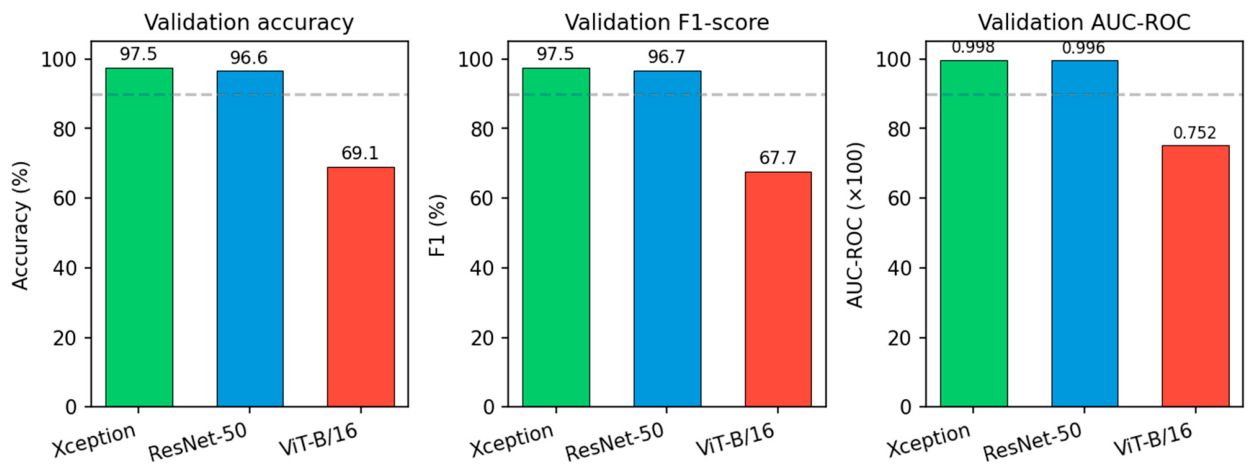
Table 1 summarizes the shared training configuration used for the compared models. Table 2 reports the best validation metrics achieved by Xception, ResNet-50, and ViT-B/16. Figure 1 and Figure 2 visualize the best achieved accuracy and the validation-accuracy trajectories across epochs for the compared models.
The evaluation protocol is as follows: for each model and each condition (clean, FGSM, PGD), the test set is forward-passed (with attack generation for adversarial conditions); accuracy, precision, recall, F1, and AUC-ROC are computed. ARI is derived from clean and adversarial accuracies. All metrics are aggregated per model and per condition so that Table 1 and Table 2 can be filled with a single value per cell (or mean ± std when multiple runs are reported).
Reporting conventions: accuracy and F1 are reported as percentages (0–100), and AUC-ROC as a value in [0, 1]. ARI is part of the RED evaluation framework and can be reported in future robustness runs with higher values indicating better robustness. The current tables focus on completed validation metrics from the clean-training baseline experiments.

5.2. Qualitative Explainability

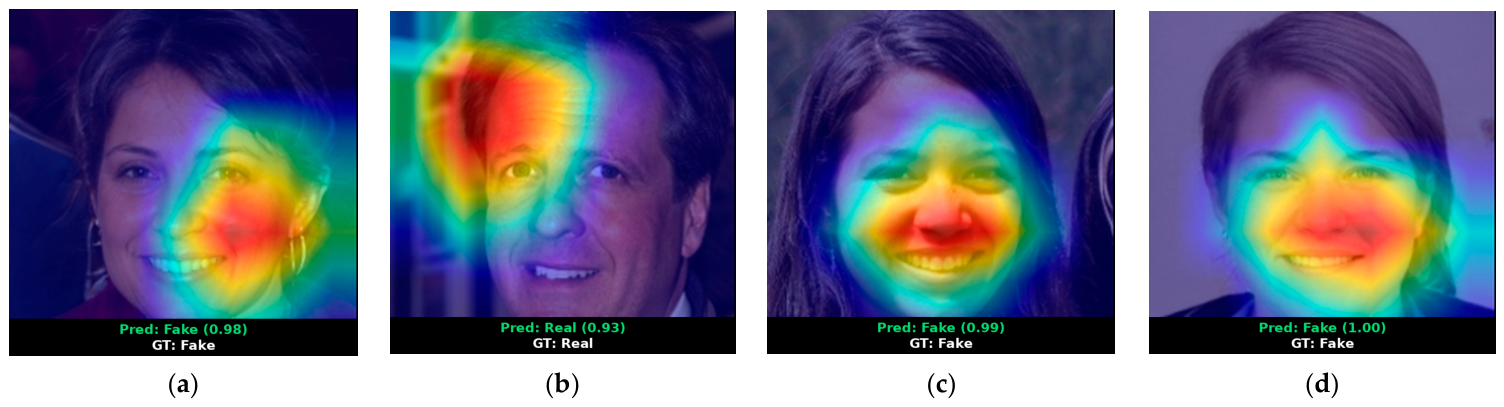
Grad-CAM heatmaps (generated by src/gradcam_viz.py) indicate spatial importance for predictions (Figure 3). In the qualitative examples shown here, the detector places most of its attention on central facial regions and local texture transitions rather than on clearly irrelevant background areas. This interpretability view serves as a diagnostic aid and supports human-in-the-loop verification. The gradcam_viz script loads a trained checkpoint, selects the appropriate target layer per architecture (last Conv2d for Xception and ResNet-50; transformer block for ViT when supported), and generates heatmaps for a configurable number of test images.
The examples in Figure 3 should be read as qualitative illustrations rather than as a completed statistical evaluation of explanation quality under attack. They are useful for checking whether attention remains visually plausible on correctly classified real and fake faces, and for identifying cases where confidence is high but localization appears questionable.
A broader comparison of heatmaps across real vs fake samples and across clean vs adversarially perturbed inputs is supported by the codebase and remains a natural extension of the present study. The gradcam_viz script allows batch generation of heatmaps for a specified number of test images so that analysts can inspect whether the model consistently attends to eyes, mouth, skin texture, or blending boundaries for fake samples.
When the model predicts correctly (e.g., Pred: Real, GT: Real, or Pred: Fake, GT: Fake), the heatmap indicates which regions supported that decision. For correctly classified real faces, concentration of activation on central facial features (eyes, nose, mouth) or natural skin texture is consistent with the model relying on plausible cues rather than background or artifacts. For correctly classified fakes, activation on boundaries, inconsistent texture, or artifact-prone regions supports the claim that the detector has learned forgery-related cues. Such alignment between heatmap localization and domain expectations (physiologically or artifact-relevant regions) supports the use of Grad-CAM as a transparency and diagnostic tool in the RED framework.

5.3. Discussion

The experiments reported here show how three baseline architectures behave on the selected dataset under a shared training protocol, while the broader RED framework defines how robustness and explainability can be evaluated in a consistent way. In that sense, the discussion centers on the current empirical findings and on what they imply for the next stage of the framework rather than making a general claim about all deepfake detectors.
The reported findings should therefore be read within the boundaries of the present setup. Higher ARI values under FGSM and PGD indicate better resistance to the specific attacks used here, but they do not automatically imply robustness to every threat model. Likewise, stronger explanation-to-mask agreement is encouraging, yet it does not by itself guarantee causal interpretability.
Reproducibility is supported by the open-source repository: data loading (data.py), model definitions (models.py), attacks (attacks.py), metrics (metrics.py), training (train.py), evaluation (eval.py), and Grad-CAM (gradcam_viz.py) are all documented and configurable via config.example.yaml and CLI. Researchers can replicate the setup, vary hyperparameters (e.g., ε, PGD steps, adv_train mode), and report results in the same table format for direct comparison.
The validation results (Table 1 and Table 2) show that:
  • Xception and ResNet-50 reach 97.53% and 96.64% validation accuracy (F1 97.51% and 96.69%, AUC-ROC 0.9977 and 0.9959) under the same clean-training protocol;
  • ViT-B/16 attains 69.08% accuracy, 67.69% F1, and 0.7521 AUC-ROC, indicating a substantial gap on this dataset under the current setup;
  • Best validation occurs at epoch 9 for Xception and ViT-B/16, and at epoch 10 for ResNet-50.
The immediate next step is to extend these baseline findings with completed FGSM/PGD robustness runs, ARI reporting, and comparison against adversarially trained or multi-stream RED variants under the same protocol.

5.4. Limitations

Failure-case analysis should examine false positives and false negatives in relation to image quality, manipulation style, and attention behavior. Such analysis is important because a detector may achieve strong average scores while still failing systematically on specific visual patterns that matter in practical deployment.
This study has several limitations. The robustness analysis is limited to L∞-bounded white-box attacks, so the results should be read as evidence about this specific evaluation setting rather than as a complete security claim. Different conclusions may emerge under transfer-based, adaptive, or black-box attacks, and robustness across datasets is likely to depend on how synthetic images are generated and post-processed.
The explanation analysis is also constrained by the available data. Metrics such as EF are most informative when manipulation masks exist and are well aligned with the image content; on datasets without reliable masks, interpretation must rely more heavily on qualitative review. In addition, Grad-CAM is applied only to compatible layers and therefore offers a partial view of the decision process, especially for transformer-based branches.
From an implementation perspective, adversarial training increases computational cost and may require careful hyperparameter tuning to avoid unnecessary clean-accuracy loss. The current experiments also focus on still images, so they do not address temporal artifacts, frame consistency, or multimodal signals that can be important in broader deepfake-detection pipelines.
Ethical considerations remain important. Systems for face analysis can support beneficial tasks such as media verification and fraud screening, but they can also be misused in surveillance-heavy or discriminatory settings. For that reason, the intended role of RED is as an assistive analytic component whose outputs should be interpreted together with human judgment, documented limitations, and appropriate governance controls.

Author Contributions

Conceptualization, G.K., P.N., and O.N.; methodology, G.K.; software, G.K.; validation, G.K. and P.N.; resources, G.K.; data curation, G.K.; writing—original draft preparation, G.K.; writing—review and editing, O.N.; visualization, G.K.; supervision, O.N.; project administration, P.N. and O.N.; funding acquisition, O.N. All authors have read and agreed to the published version of the manuscript.

Funding

The research work presented in this paper was funded by the European Union-NextGenerationEU via the National Recovery and Resilience Plan of the Republic of Bulgaria under project BG-RRP-2.004-0005 “Improving the research capacity and quality to achieve international recognition and resilience of TU-Sofia (IDEAS)”. The research that led to these results was carried out using the infrastructure purchased under the National Roadmap for RI, financially coordinated by the MES of the Republic of Bulgaria (grant no. DO1-98/26.06.2025).

Institutional Review Board Statement

Not applicable.

Informed Consent Statement

Not applicable.

Data Availability Statement

Data are contained within the article. The repository used for the training is hosted at https://github.com/MrKotov/face-explainability (accessed on 15 March 2026).

Conflicts of Interest

The authors declare no conflicts of interest.

Abbreviations

The following abbreviations are used in this manuscript:
AIArtificial Intelligence
ARIAdversarial Robustness Index
AUC-ROCArea Under the Receiver Operating Characteristic Curve
CNNConvolutional Neural Network
EFExplainability Fidelity
FGSMFast Gradient Sign Method
GANGenerative Adversarial Network
Grad-CAMGradient-weighted Class Activation Mapping
IGIntegrated Gradients
LRPLayer-wise Relevance Propagation
PGDProjected Gradient Descent
REDRobust and Explainable Detection
ViTVision Transformer
XAIExplainable Artificial Intelligence
CLICommand-Line Interface
CSVComma-Separated Values
FFTFast Fourier Transform
MLMachine Learning
ROCReceiver Operating Characteristic

References

  1. Goodfellow, I.J.; Pouget-Abadie, J.; Mirza, M.; Xu, B.; Warde-Farley, D.; Ozair, S.; Courville, A.; Bengio, Y. Generative adversarial networks. Adv. Neural Inf. Process. Syst. 2014, 15, 2672–2680. [Google Scholar] [CrossRef]
  2. Ho, J.; Jain, A.; Abbeel, P. Denoising diffusion probabilistic models. Adv. Neural Inf. Process. Syst. 2020, 33, 6840–6851. [Google Scholar] [CrossRef]
  3. He, K.; Zhang, X.; Ren, S.; Sun, J. Deep residual learning for image recognition. In IEEE/CVF Conference on Computer Vision and Pattern Recognition; IEEE: New York, NY, USA, 2016; pp. 770–778. [Google Scholar] [CrossRef]
  4. Dosovitskiy, A.; Beyer, L.; Kolesnikov, A.; Weissenborn, D.; Zhai, X.; Unterthiner, T.; Dehghani, M.; Minderer, M.; Heigold, G.; Gelly, S.; et al. An image is worth 16 × 16 words: Transformers for image recognition at scale. arXiv 2021, arXiv:2010.11929. [Google Scholar] [CrossRef]
  5. Vaswani, A.; Shazeer, N.; Parmar, N.; Uszkoreit, J.; Jones, L.; Gomez, A.N.; Kaiser, Ł.; Polosukhin, I. Attention is all you need. In Proceedings of the Advances in Neural Information Processing Systems, Long Beach, CA, USA, 4–9 December 2017; Volume 30. [Google Scholar] [CrossRef]
  6. Rössler, A.; Cozzolino, D.; Verdoliva, L.; Riess, C.; Thies, J.; Nießner, M. FaceForensics++: Learning to detect manipulated facial images. In Proceedings of the IEEE International Conference on Computer Vision, Seoul, Republic of Korea, 27 October–2 November 2019; pp. 1–11. [Google Scholar] [CrossRef]
  7. Lin, L.; Santosh, S.; Wu, M.; Wang, X.; Hu, S. AI-Face: A million-scale demographically annotated AI-generated face dataset and fairness benchmark. In IEEE/CVF Conference on Computer Vision and Pattern Recognition; IEEE: New York, NY, USA, 2025. [Google Scholar] [CrossRef]
  8. Goodfellow, I.J.; Shlens, J.; Szegedy, C. Explaining and harnessing adversarial examples. arXiv 2015, arXiv:1412.6572. [Google Scholar] [CrossRef]
  9. Madry, A.; Makelov, A.; Schmidt, L.; Tsipras, D.; Vladu, A. Towards deep learning models resistant to adversarial attacks. arXiv 2018, arXiv:1706.06083. [Google Scholar] [CrossRef]
  10. Szegedy, C.; Zaremba, W.; Sutskever, I.; Bruna, J.; Erhan, D.; Goodfellow, I.; Fergus, R. Intriguing properties of neural networks. arXiv 2014, arXiv:1312.6199. [Google Scholar] [CrossRef]
  11. Moosavi-Dezfooli, S.-M.; Fawzi, A.; Frossard, P. DeepFool: A simple and accurate method to fool deep neural networks. In IEEE/CVF Conference on Computer Vision and Pattern Recognition; IEEE: New York, NY, USA, 2016; pp. 2574–2582. [Google Scholar] [CrossRef]
  12. Papernot, N.; McDaniel, P.; Goodfellow, I.; Jha, S.; Celik, Z.B.; Swami, A. Practical black-box attacks against machine learning. In ACM Asia Conference on Computer and Communications Security; Association for Computing Machinery: New York, NY, USA, 2017; pp. 506–519. [Google Scholar] [CrossRef]
  13. Selvaraju, R.R.; Cogswell, M.; Das, A.; Vedantam, R.; Parikh, D.; Batra, D. Grad-CAM: Visual explanations from deep networks via gradient-based localization. In IEEE International Conference on Computer Vision; IEEE: New York, NY, USA, 2017; pp. 618–626. [Google Scholar] [CrossRef]
  14. Bach, S.; Binder, A.; Montavon, G.; Klauschen, F.; Müller, K.-R.; Samek, W. On pixel-wise explanations for non-linear classifier decisions by layer-wise relevance propagation. PLoS ONE 2015, 10, e0130140. [Google Scholar] [CrossRef] [PubMed]
  15. Sundararajan, M.; Taly, A.; Yan, Q. Axiomatic attribution for deep networks. In International Conference on Machine Learning; PMLR: Cambridge, MA, USA, 2017; pp. 3319–3328. [Google Scholar] [CrossRef]
  16. Chefer, H.; Singh, S.; Guestrin, C. Transformer interpretability beyond attention visualization. In IEEE/CVF Conference on Computer Vision and Pattern Recognition; IEEE: New York, NY, USA, 2021; pp. 782–791. [Google Scholar] [CrossRef]
  17. Ribeiro, M.T.; Singh, S.; Guestrin, C. “Why should I trust you?” Explaining the predictions of any classifier. In Proceedings of the ACM SIGKDD Conference on Knowledge Discovery and Data Mining, San Francisco, CA, USA, 13–17 August 2016; pp. 1135–1144. [Google Scholar] [CrossRef]
  18. Lundberg, S.M.; Lee, S.-I. A unified approach to interpreting model predictions. In Advances in Neural Information Processing Systems; Curran Associates, Inc.: Red Hook, NY, USA, 2017; Volume 30. [Google Scholar] [CrossRef]
  19. Petsiuk, V.; Das, A.; Saenko, K. RISE: Randomized input sampling for explanation of black-box models. arXiv 2018, arXiv:1806.07421. [Google Scholar] [CrossRef]
  20. Cohen, J.; Rosenfeld, E.; Kolter, Z. Certified adversarial robustness via randomized smoothing. In International Conference on Machine Learning; IEEE: New York, NY, USA, 2019; pp. 1310–1320. [Google Scholar] [CrossRef]
  21. Jaccard, P. The distribution of the flora in the alpine zone. New Phytol. 1912, 11, 37–50. [Google Scholar] [CrossRef]
  22. Chollet, F. Xception: Deep learning with depthwise separable convolutions. In Proceedings of the IEEE/CVF Conference on Computer Vision and Pattern Recognition, Honolulu, HI, USA, 21–26 July 2017; pp. 1251–1258. [Google Scholar] [CrossRef]
  23. Wightman, R. PyTorch Image Models. 2019. Available online: https://github.com/rwightman/pytorch-image-models (accessed on 1 March 2026).
  24. Russakovsky, O.; Deng, J.; Su, H.; Krause, J.; Satheesh, S.; Ma, S.; Huang, Z.; Karpathy, A.; Khosla, A.; Bernstein, M.; et al. ImageNet large scale visual recognition challenge. Int. J. Comput. Vis. 2015, 115, 211–252. [Google Scholar] [CrossRef]
  25. Deng, J.; Dong, W.; Socher, R.; Li, L.-J.; Li, K.; Fei-Fei, L. ImageNet: A large-scale hierarchical image database. In Proceedings of the IEEE Conference on Computer Vision and Pattern Recognition, Miami, FL, USA, 20–25 June 2009; pp. 248–255. [Google Scholar] [CrossRef]
  26. Paszke, A.; Gross, S.; Massa, F.; Lerer, A.; Bradbury, J.; Chanan, G.; Killeen, T.; Lin, Z.; Gimelshein, N.; Antiga, L.; et al. PyTorch: An imperative style, high-performance deep learning library. In Advances in Neural Information Processing Systems; Curran Associates, Inc.: Red Hook, NY, USA, 2019; Volume 32. [Google Scholar] [CrossRef]
  27. Pan, S.J.; Yang, Q. A survey on transfer learning. IEEE Trans. Knowl. Data Eng. 2010, 22, 1345–1359. [Google Scholar] [CrossRef]
  28. Bishop, C.M. Pattern Recognition and Machine Learning; Springer: Berlin/Heidelberg, Germany, 2006; ISBN 978-0-387-31073-2. [Google Scholar]
  29. Kingma, D.P.; Ba, J. Adam: A method for stochastic optimization. arXiv 2015, arXiv:1412.6980. [Google Scholar] [CrossRef]
  30. Pedregosa, F.; Varoquaux, G.; Gramfort, A.; Michel, V.; Thirion, B.; Grisel, O.; Blondel, M.; Prettenhofer, P.; Weiss, R.; Dubourg, V.; et al. Scikit-learn: Machine learning in Python. J. Mach. Learn. Res. 2011, 12, 2825–2830. [Google Scholar] [CrossRef]
  31. Fawcett, T. An introduction to ROC analysis. Pattern Recognit. Lett. 2006, 27, 861–874. [Google Scholar] [CrossRef]
Figure 1. Accuracy percentage between models in the best epoch.
Engproc 150 00052 g001
Figure 2. Validation Accuracy across different models.
Engproc 150 00052 g002
Figure 3. Grad-CAM visualizations for the proposed detector for four photos (a–d): hot regions indicate where the model attended for its prediction (real or fake). Labels on each panel give the predicted class, confidence, and ground truth (GT), allowing interpretation of both correct and misclassified cases. (a) Properly predicted fake photo #1; (b) properly predicted real photo #2; (c) properly predicted fake photo #3; (d) properly predicted fake photo #4.
Engproc 150 00052 g003
Table 1. Xception, ResNet-50, and ViT-B/16 models’ training configuration.
ParameterValue
Epochs10
Batch size32
Learning rate0.0003
Max samples per epoch2000
Adversarial trainingnone
ε (0–255)8
α (PGD)2
PGD steps5
Seed42
Table 2. Xception, ResNet-50, and ViT-B/16 models’ best validation metric summary.
MetricXceptionResNet50ViT-B16
Best epoch9109
Accuracy (%)97.5396.6469.08
F1 (%)97.5196.6967.69
AUC-ROC0.99770.99590.7521
Disclaimer/Publisher’s Note: The statements, opinions and data contained in all publications are solely those of the individual author(s) and contributor(s) and not of MDPI and/or the editor(s). MDPI and/or the editor(s) disclaim responsibility for any injury to people or property resulting from any ideas, methods, instructions or products referred to in the content.