


Abstract
UAVs operating in cluttered and dynamic environments face limitations when controlled using conventional Euclidean frameworks, which leads to degraded performance during aggressive maneuvers. This paper presents a geometry-aware predictive control framework for multirotor UAVs based on a two-manifold-inspired representation of actuator geometry. The proposed control strategy adopts an MPC-inspired prediction structure without solving a full online optimization problem. A comparative simulation study is conducted in MATLAB/Simulink under identical mission, obstacle, and noise conditions for both the conventional point-mass controller and the proposed two-manifold-based controller. Performance is evaluated in terms of trajectory tracking accuracy and control effort. Results indicate that the proposed framework achieves modest improvements in tracking accuracy and produces smoother control inputs compared to the point-mass model. It suggests that geometry-aware representations may enhance predictive control performance in obstacle-rich environments, although further validation under diverse scenarios is required.
1. Introduction
Unmanned Aerial Vehicles (UAVs) are integral to a wide range of civilian and industrial applications. As the autonomy and operational envelope of UAVs expand, control strategies must cope with nonlinear dynamics, actuator constraints, environmental disturbances, and state-estimation uncertainties [1,2,3]. Among several approaches, Model Predictive Control (MPC) is widely used due to its ability to explicitly incorporate prediction, multivariable coupling, and constraints into the control loop [1,4]. MPC has been applied to UAV trajectory tracking, disturbance rejection, cooperative control, and autonomous landing in both linear and nonlinear formulations [2,3]. The literature indicates that MPC can provide improved performance compared to classical methods such as PID and LQR when operating under constraints and in dynamically evolving environments [1,5,6]. However, the overwhelming majority of MPC-based UAV controllers adopt point-mass system representations, in which the UAV is modelled about its centre of gravity (CG) using position, velocity, and attitude states [1,7].
While point-mass models are simple to design and reduce computational cost, they introduce certain inherent limitations. The separation of translational and rotational dynamics necessitates cascaded or hierarchical control architectures, as well as nonlinear mapping functions. These mappings can be sensitive to modelling inaccuracies, actuator saturation, and aggressive maneuvers, thereby limiting estimation fidelity and closed-loop performance—particularly during disturbances or fault conditions [1,8,9]. As a result, the quality of prediction in predictive control frameworks remains influenced by the abstraction imposed by the point-mass model [7,9].
Recent work has explored alternative modelling paradigms that relax the point-mass assumption. A notable direction is a geometry-based representation in which the UAV is approximated using multiple vertices corresponding to rotor locations, with constraints imposed on their relative geometry [9]. In this study, this representation is referred to as a two-manifold-inspired model, where the term “manifold” is used in a geometric approximation sense rather than as a strict continuous mathematical surface.
In this representation, control inputs are distributed across actuator-associated vertices instead of being applied solely at the CG. This enables a more direct relationship between geometry and actuation and may reduce reliance on intermediate control allocation mappings. From a predictive control perspective, such representations can improve consistency between the internal model and actuator-level behaviour.
Motivated by these observations, this work investigates a geometry-aware predictive control framework based on a two-manifold representation. The proposed approach adopts an MPC-inspired structure that incorporates prediction horizons without solving a full online optimization problem. A comparative study is conducted against a conventional point-mass controller under identical operating conditions to evaluate differences in tracking accuracy and control effort. The objective of this study is to assess whether geometry-aware representations can provide measurable improvements in predictive control performance under obstacle-rich conditions.
2. Methodology
The objective of this study is to compare a geometry-aware two-manifold-based control strategy against a conventional point-mass controller under identical operating conditions. Both controllers are executed on the same quadrotor dynamic model, sharing identical mass properties, actuator parameters, noise characteristics, reference trajectories, and evaluation metrics. To ensure a fair comparison, controller gains, constraints, and simulation conditions are kept consistent wherever applicable. The primary conceptual difference between the two approaches lies in the control representation. In the point-mass controller, control inputs are computed at the CG and subsequently mapped to motor commands through attitude mixing. In contrast, the geometry-aware controller computes control actions directly in vertex space, where each actuator corresponds to a discrete geometric vertex associated with the rotor locations. This approach ensures that any observed performance differences can be attributed to the control representation rather than differences in system modelling, parameter selection, or tuning. The comparison focuses on the effect of modelling representation on system behaviour under a fixed control structure. Algorithm 1 outlines the parallel implementation of both control strategies within the MATLAB/Simulink (Version R2026a, MathWorks, Natick, MA, USA). The simulation using Algorithm 1 was validation was completed using the custom-built script, Matlab Code S1: Ver_Final.m.
| Algorithm 1: Parallel Execution of Point-Mass and two-manifold-based Controllers |
| Input: Initial state , reference trajectory , system parameters , controller gains , horizons Output: State trajectories, control inputs, RMSE, control effort, per-vertex metrics Initialization
For to do 1. Reference Update
(A) Point-Mass Controller
|
Consider a quadrotor UAV with n = 4 motors operating in a three-dimensional space. The UAV is typically modelled as a point-mass system with six DoFs, consisting of three translational components (position) and three rotational components (orientation). The motion of the UAV evolves due to the thrust generated by its propellers. Each motor produces thrust based on an input signal. In practice, these inputs are bounded such that the input lies between the minimum and maximum due to actuator saturation. These limits define the feasible operating range of the system dynamics. While the dynamics are modelled at the CG, a geometric representation of the UAV structure is incorporated through a rigid-body transformation. The pose of the UAV is represented using a rotation matrix R ∈ ℝ3×3 and position vector p ∈ ℝ3, defining a homogeneous transformation T. At any instant, the pose of the UAV is described by its position and its orientation represented by a rotation matrix R. Together, these define the transformation that maps points from the body frame to the world frame. Since the CG is treated as a point, the system has six degrees of freedom given by DoFs = 3 (position) + 3 (orientation) = 6. To incorporate the physical structure, the quadrotor is modelled with four fixed vertices corresponding to the motor locations. Each motor is positioned at a constant arm length L from the CG, forming a rigid planar geometry. In the body frame, the position of the i-th motor can be written relative to the CG, as cosine and sine multiples of the arm length L, and does not have a third coordinate. Because the motor is in a two-dimensional hyperplane in 3D Euclidean space. Thus, each motor position shall be a vertex, and its homogeneous matrix contains the identity matrix and two coordinates relative to the CG. Upon multiplication, the resultant transformation matrix of the vertex has R, and the orientation of CG is retained. The position of each motor in the world frame is obtained using a rigid transformation given by V_i = R r_i + p. In this expression, the rotation matrix R applies the same orientation to all motor positions, while the vector p translates the entire structure in space. Because the relative distances between CG and the motor remain constant, the quadrotor behaves as a rigid body. Although the system is represented by multiple points, these are completely determined by the same underlying variables (R, p). Therefore, no additional independent motion is introduced, and the system remains six-dimensional.
This formulation provides geometric consistency without explicitly modelling detailed rotational dynamics. The orientation encoded in R is implicitly reflected in the positions of all vertices, ensuring that the entire structure moves coherently. As a result, the motion of the CG is mapped into n spatial points while preserving the rigid-body nature of the quadrotor. From a dimensionality and degrees-of-freedom perspective, the system remains a 6-DoF rigid body. For 3D Euclidean space, if dimensionality D is 3, then DoF is 6 as D(D + 1)/2. Thus, although the system is embedded in a higher-dimensional Euclidean space for four vertices in ℝ3, the effective system dimensionality remains constrained by the underlying rigid-body motion.
The state vector based on observable parameters like position and velocity in Euclidean space is defined as Equation (1), where p = [x, y, z]T denotes the position of the centre of gravity (CG) and v = [vx, vγ, v𝓏]T denotes the velocity. The continuous-time system dynamics are given by ṗ = v, and is defined in Equation (2), where Fv ∈ ℝ3 represents the resultant thrust expressed in the world frame, m is the UAV mass, and g = [0, 0, g]T denotes the gravitational acceleration vector.
x = [pT vT]T = [x y z vx vᵧ v𝓏]T
The system is discretised using forward Euler integration with sampling time Ts = 0.01 s, and the state prediction equation is given by Equation (3).
Zero-mean Gaussian process noise with a standard deviation of 0.5 m/s2 is added to the acceleration states. To ensure physically realistic motion, the magnitude of the velocity is constrained to ‖vk‖ ≤ 8.5 m/s.
In the point-mass control strategy, the UAV is treated as a single rigid particle located at its CG. Control inputs are expressed in terms of total thrust T, roll angle φ, pitch angle θ, and yaw angle ψ. A PID-based state feedback controller in Equation (4) computes the desired translational acceleration. No receding horizon optimization problem is solved online; therefore, this approach differs from conventional MPC.
where the position and velocity errors are given by Equation (5) and Equation (6), respectively.
a = Kp ep + K𝒹 ev + Ki ∫ ep dt
ep = pref − p
ev = −v
The desired acceleration is mapped to attitude and thrust commands using small-angle approximations given in Equations (7)–(9).
θ = ax/g
φ = −aγ/g
T = m (g + a𝓏)
Motor-level Pulse Width Modulation (PWM) commands are obtained via a standard Quad-X motor mixing scheme, with proportional stabilization gains applied for roll, pitch, and yaw. For implementation clarity, gravity compensation is inherently included in Equation (2) through the constant term g. The controller generates motor commands as raw PWM values bounded within the range 110–220. These values are subsequently mapped to actuator-level thrust using a normalized scaling within the actuator model, where PWM signals are internally scaled by the factor u/255 to obtain equivalent motor voltage [4].
The proposed approach represents the UAV using four discrete vertices corresponding to the physical rotor locations, forming a rigid geometric structure with fixed inter-vertex distance [4]. Each vertex is defined in the body frame and transformed into the world frame using a rigid-body homogeneous transformation. T(p, ψ) in Equation (10) denotes the homogeneous transformation parameterized by the UAV position p and yaw angle ψ. Control is performed directly in vertex space using Equation (11). For each vertex, a directional tracking error is computed by projecting the displacement between reference and actual vertex positions onto the outward unit normal vector . Independent PID controllers are applied to each vertex to generate incremental motor-level control signals using Equation (12). All key parameters used in the simulation are tabulated in Table 1, along with PID parameters. PID gain values are obtained empirically through iterative tuning, with the objective of achieving stable and asymptotic tracking performance in simulation. The tuning process is guided by minimizing steady-state error and ensuring acceptable transient behaviours, including limited overshoot and satisfactory settling time. Both controllers use identical PID gains, actuator limits, noise models, and dynamic assumptions, ensuring that performance differences arise solely from the control representation rather than tuning or implementation variations.
Vi = T(p, ψ) · vi
Table 1.
Key Parameters used in simulation.
This formulation enables geometry-aware distributed control, where coupling between translational and rotational effects is approximated through the geometric structure and thrust distribution across vertices. Although prediction horizons and cost functions are defined, the full finite-horizon optimization problem is not solved online. Therefore, the proposed approach is more accurately characterized as an MPC-inspired predictive control strategy rather than a conventional MPC implementation. The prediction and control horizons are defined as Np = 30, Nu = 10, with weighting matrices Qp = diag(8, 8, 12), and Ru = 0.02 I. For CG motion, the quadratic cost function is defined as Equation (13).
J = Σk=1Np ‖pk − pref,k‖2 Qp + Σk=1Nu ‖uk‖2 Ru
For the two-manifold controller, the cost is evaluated in vertex space using Equation (14).
Jv = Σk=1Np Σi=14 ‖Vi,k − Vi,kref‖2
Prediction horizons for both the CG and per-vertex trajectories are logged at every control step for post-analysis. The simulated environment includes both static and dynamic obstacles. Static obstacles are modelled as vertical cylindrical structures located at (±15 m, ±15 m), each with a radius of 3.5 m and a height of 56 m. Dynamic obstacles are modelled as spherical objects with a radius of 1.2 m, following sinusoidal trajectories within ±60 m spatial bounds and ±3 m altitude variation around the cruise level. Obstacle perception is limited to a sensing radius of 10 m, with Gaussian noise (0.8, 0.8, 0.6) m in the x, y, and z directions and a missed detection probability of 0.10. Clearance is defined as the minimum Euclidean distance between the UAV and the obstacle surface. Obstacle perception is constrained by a limited sensing radius—rsense = 10 m. Detected obstacle positions are subjected to Gaussian noise, and a missed-detection probability of Pmiss = 0.10 is applied. Only perceived obstacles influence avoidance behaviour. Braitenberg behaviour is implemented through directional error projection at each actuator location, where the displacement between reference and actual vertex positions is projected onto an outward unit vector. This produces a local stimulus-response mapping, which directly modulates motor inputs without intermediate planning. Activation of this behaviour is detected when the projected error falls below a defined buffer threshold.
In the present framework, prediction horizons (Np and Nu) and cost functions are defined to provide a structured basis for performance evaluation and trajectory analysis. However, no finite-horizon optimization problem is solved online. Control inputs in both the point-mass and two-manifold-based controllers are generated using PID-based feedback laws derived from instantaneous tracking errors. The prediction mechanism operates as a parallel analytical layer, in which future state and vertex trajectories are estimated and associated costs are evaluated at each time step. These predicted trajectories and cost values are not used to update the control input. Instead, they serve as diagnostic tools that allow consistent comparison of control behaviour, tracking performance, and geometry-induced effects across both modelling approaches. This design choice ensures a controlled comparison between the point-mass and two-manifold-based representations under identical feedback control structures. Introducing optimization-based MPC would change the controller class and confound the comparison, making it difficult to isolate the effect of geometric representation. However, it is important to note that all similarities do not guarantee an equivalent comparison, since the two controllers operate in different control spaces. The point-mass controller computes errors at the CG, whereas the two-manifold-based controller operates on vertex-level projected errors with distributed actuation.
Trajectory tracking performance is evaluated using the root mean square error (RMSE) in Equation (15).
The control effort is quantified as Equation (16).
Additional metrics include per-vertex RMSE and settling time defined using a 2% error tolerance band. Control smoothness is evaluated indirectly through the temporal variation in PWM signals and stage cost evolution. The two-manifold-based approach exhibits reduced high-frequency oscillations in both error trajectories and control inputs, indicating smoother system behaviour compared to the point-mass model. The cost function consists of a quadratic position tracking error term and a control effort penalty proportional to the squared motor inputs. This formulation allows direct comparison of tracking performance and actuation efficiency between the two approaches.
In addition to tracking performance, obstacle avoidance safety is evaluated using the minimum clearance metric. The minimum clearance is defined as the smallest Euclidean distance between the UAV and surrounding obstacles, adjusted by obstacle radius, computed over the entire simulation horizon. The minimum clearance is defined as Equation (17). Where pk is the UAV position and robs is the obstacle radius.
3. Results and Discussions
A full closed-loop simulation was conducted for 60 s with a sampling time of Ts = 0.01 s, resulting in 6000 discrete steps. The system operated continuously under Braitenberg-style obstacle avoidance, which remained active throughout the entire simulation. At intervals [0.00, 59.98]: during take-off to landing, dynamic obstacles were encountered. The minimum obstacle clearance was explicitly computed throughout the mission by evaluating the distance between the UAV and each obstacle at each simulation step. A near-collision event is defined as clearance below 0.5 m. The results show that the minimum clearance remained strictly positive, with values of 6.967 m for the two-manifold-based controller and 6.936 m for the point-mass controller. No collision or near-collision events were observed, confirming safe operation under continuous Braitenberg-style avoidance. This also leads to a potential hypothesis that the obstacle-avoidance mechanism did not merely rely on implicit safety margins but maintained measurable geometric separation throughout execution. In both approaches, Braitenberg logic follows the same underlying principle of directly mapping the tracking error to control inputs without intermediate planning or optimization.
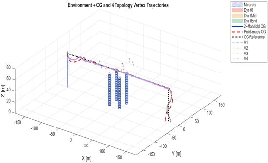
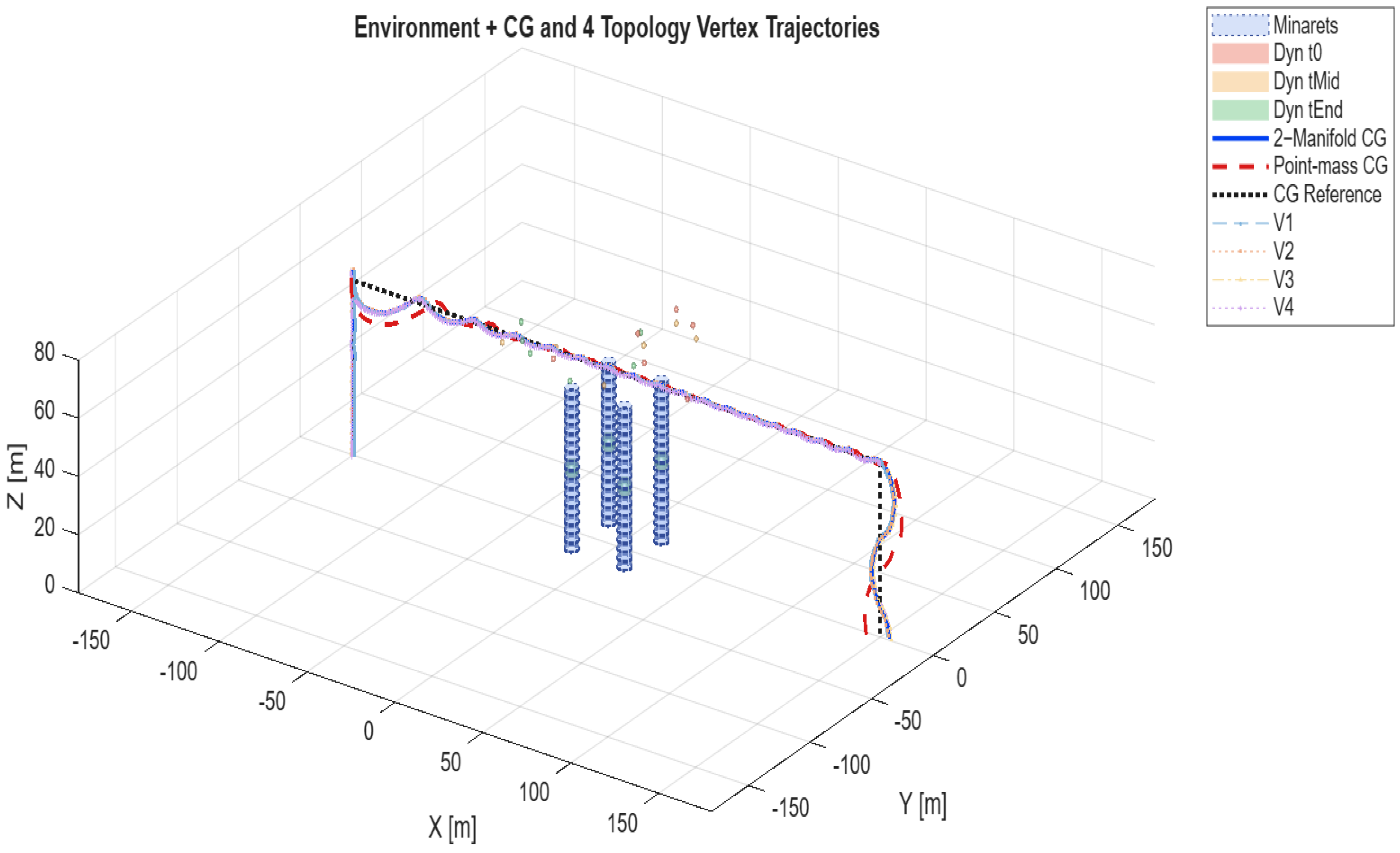
The key distinction, however, lies in where this mapping is applied. In the point-mass approach, the mapping is performed at a single global level using the CG, resulting in a centralized response where all actuators respond uniformly to a common error signal. In contrast, the two-manifold approach distributes this mapping across multiple vertices, where each vertex generates its own local response based on directional error, forming a distributed control mechanism. This transition from centralized to distributed mechanism alters the system behaviour, where the two-manifold demonstrates a potential for smoother and more coordinated motion due to spatially resolved control. The spatial behaviours of the UAV in a cluttered three-dimensional environment are illustrated in Figure 1, which shows the environment, obstacles (minarets), and the resulting trajectories of the two-manifold and point-mass models. This result highlights a key advantage of the two-manifold formulation, viz., forces are spatially distributed across the vehicle topology rather than being applied at a single point. Table 2 presents the performance-based metrics extracted from the simulation, which quantitatively support observations. It must be noted that the input effort values for V1–V4 represent per-vertex contributions in the two-manifold-based formulation. The total input effort for the two-manifold-based model is obtained by summing these values across all vertices, resulting in a total effort of 101,898. The observed performance differences reflect the combined influence of control representation and error formulation rather than geometric representation alone. No formal gain-sensitivity or robustness analysis was conducted in this study, and this remains an area for future investigation.
Figure 1.
Environment, obstacles (minarets), and the resulting trajectories of the two-manifold and point-mass models.
Table 2.
Performance metrics summary.
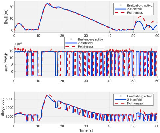
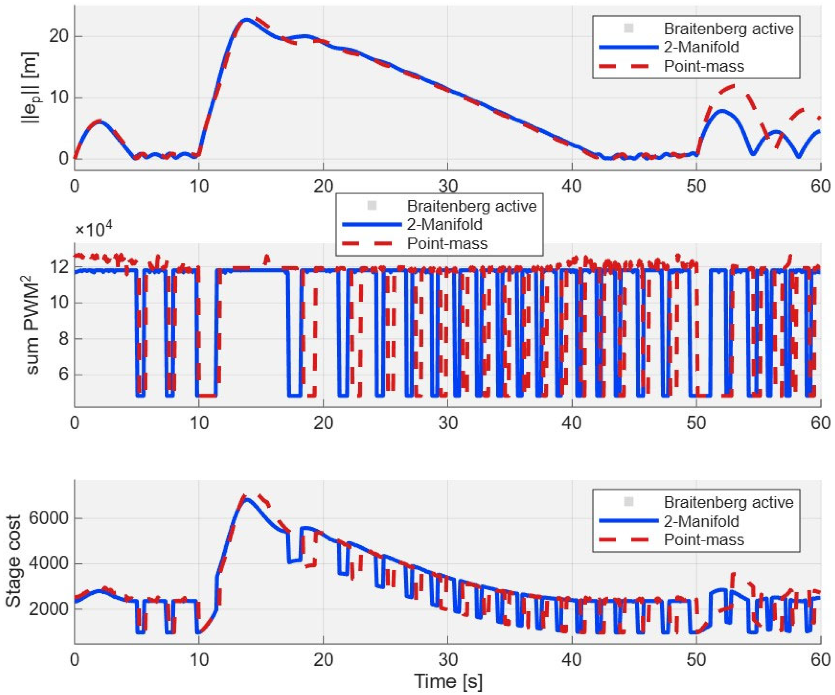
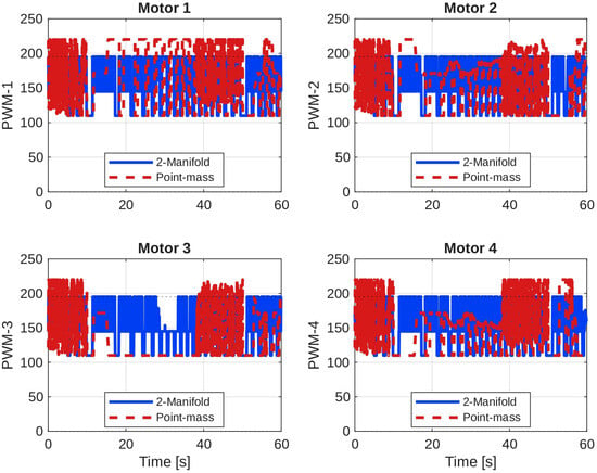
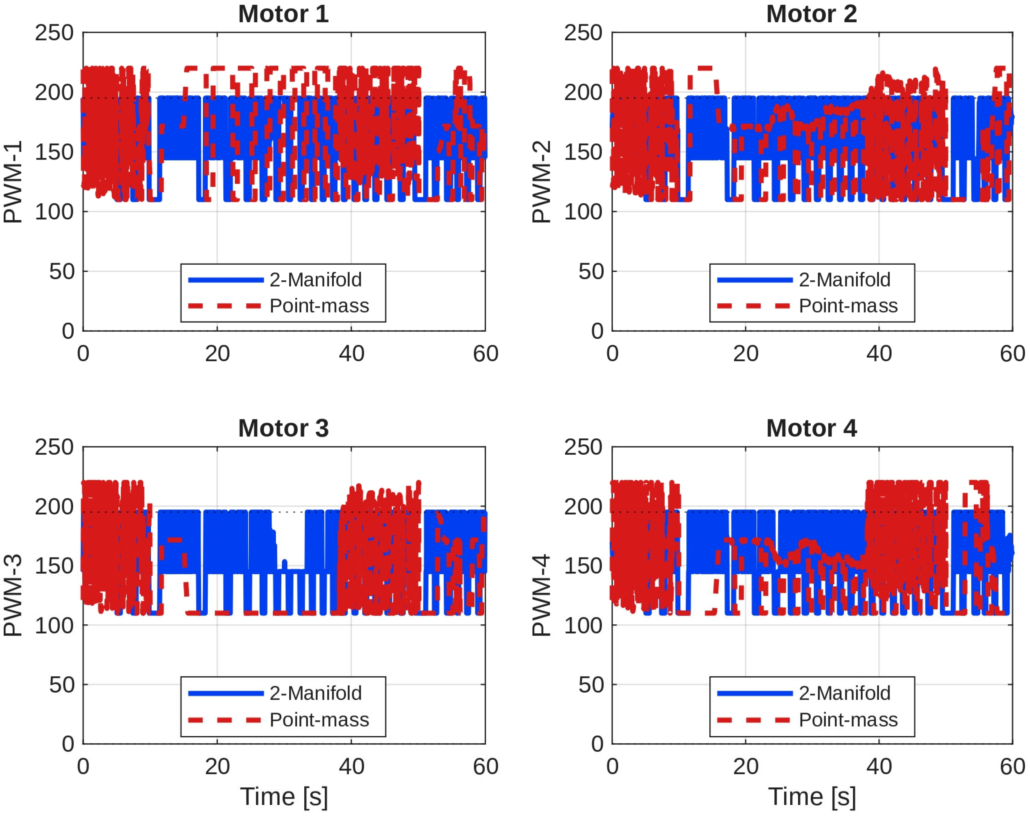
Each vertex of the proposed model achieves nearly identical RMSE values (≈10.64 m), indicating uniform tracking quality across the structure. The average RMSE (10.641 m) is lower than the point-mass CG RMSE (10.898 m), corresponding to an approximate reduction of 2.4%. The total input-effort metric also shows a small reduction of approximately 1.1% relative to the point-mass controller. All vertices and the point-mass CG exhibit settling times equal to the simulation horizon (59.98 s), indicating that neither controller reaches a conventional steady-state under continuous Braitenberg-style avoidance. Therefore, stability should be interpreted in terms of bounded tracking behaviour rather than classical settling performance. The accumulated cost and tracking error evolution are shown in Figure 2. The proposed model exhibits a smoother variation in cost and control signals compared to the point-mass formulation. This suggests that the distributed control structure can moderate abrupt control actions by redistributing actuator demand across vertices. Similarly, the PWM profiles shown in Figure 3 indicate lower peak values and smoother temporal variation for the proposed controller. This corresponds to a reduction in the summed squared control-input metric rather than direct energy consumption.
Figure 2.
Performance for the entire mission.
Figure 3.
PWM comparison for four motors (two-manifold-based vs. point-mass models).
Such characteristics may indicate less aggressive actuation and smoother operation; however, actuator stress, energy consumption, and hardware-level effects are not explicitly modelled in this study. The reported results are based on a single simulation scenario and should be interpreted as preliminary. Additional simulations under varied conditions would be required to establish generality.
Overall, the results suggest that the two-manifold-inspired representation provides modest but consistent improvements in tracking accuracy and produces smoother control inputs compared to the point-mass formulation. While the quantitative differences are relatively small, they indicate that incorporating geometric structure at the actuator level may improve the consistency between the system representation and control action. It is important to emphasize that the observed performance differences are attributed to the modelling and control representation rather than changes in controller design. Further validation under diverse scenarios is required to draw stronger conclusions regarding robustness and practical applicability.
4. Conclusions
This work presented a geometry-aware predictive control framework for multirotor UAVs that departs from conventional point-mass representations by incorporating a vertex-based geometric structure associated with actuator locations. A comparative simulation study was conducted between a conventional point-mass controller and a two-manifold-inspired predictive control strategy under identical mission profiles, environmental conditions, actuator constraints, and noise characteristics. The only distinguishing factor was the control representation: CG control versus vertex-level control, ensuring a fair basis for comparison. The results indicate that the proposed geometry-aware framework achieves modest improvements in trajectory tracking accuracy and produces smoother control inputs compared to the point-mass approach. While the observed differences are relatively small, they are consistent across the simulation scenario and suggest potential advantages of distributing control actions across actuator-associated vertices. The study highlights that predictive control performance is influenced by the underlying system representation. In this regard, the proposed two-manifold-inspired representation provides a structured way to incorporate actuator-level geometry into the control process. However, since full rigid-body rotational dynamics and online optimization are not explicitly modelled, the approach is more accurately characterized as an MPC-inspired predictive control framework. Safety metrics such as minimum obstacle clearance, collision count, and near-collision events are not explicitly quantified in this study and remain part of future work.
Overall, the findings suggest that geometry-aware representations may enhance predictive control behaviours in obstacle-rich environments, although further validation is required. Future work will focus on extending this framework to more comprehensive dynamic models, conducting extensive simulation studies under varied conditions, and validating performance through real-time or hardware-based implementations.
Supplementary Materials
The following supporting information can be downloaded at: https://doi.org/10.5281/zenodo.19880702 (accessed on 23 June 2026), Matlab Code S1: Ver_Final.m.
Author Contributions
Conceptualization, Y.G.; methodology, Y.G.; software, Y.G.; validation, Y.G. and M.S.K.; formal analysis, Y.G.; investigation, M.S.K.; resources, M.S.K.; data curation, Y.G.; writing—original draft preparation, Y.G.; writing—review and editing, Y.G. and M.S.K.; visualization, Y.G.; supervision, M.S.K.; project administration, M.S.K. All authors have read and agreed to the published version of the manuscript.
Funding
This research received no external funding.
Institutional Review Board Statement
Not applicable.
Informed Consent Statement
Not applicable.
Data Availability Statement
The original source code can be downloaded at https://doi.org/10.5281/zenodo.19880702 (accessed on 23 June 2026), Matlab Code S1: Ver_Final.m.
Acknowledgments
During the preparation of this manuscript/study, the authors used Co-pilot for the purposes of paraphrasing, spell checking, and debugging the original source code. The authors have reviewed and edited the output and take full responsibility for the content of this publication.
Conflicts of Interest
The authors declare no conflicts of interest.
Abbreviations
The following abbreviations are used in this manuscript:
| UAV | Unmanned Aerial Vehicle |
| CG | Centre of Gravity |
| PID | Proportional–Integral–Derivative |
| RMSE | Root Mean Square Error |
| PWM | Pulse Width Modulation |
| TCL | Takeoff–Cruise–Landing |
| DoF | Degrees of Freedom |
| V1–V4 | Vertices 1 to 4 of the Two-Manifold-Based Model |
| Vavg | Average of Manifold Vertices |
| VCG | Centre-of-Gravity State (Point-Mass Model) |
| Ts | Sampling Time |
| Np | Prediction Horizon |
| Nu | Control Horizon |
| Qp | State (Position) Weighting Matrix |
| Ru | Control Input Weighting Matrix |
| Fv | Resultant Thrust Vector |
| g | Gravitational Acceleration |
| φ | Roll Angle |
| θ | Pitch Angle |
| ψ | Yaw Angle |
| Quad-X | Quadrotor Motor Configuration |
| Unit Normal Vector at Vertex i | |
| ei | Vertex-Level Tracking Error |
| ℝ3 | Three-Dimensional Real Space |
References
- Panjavarnam, K.; Ismail, Z.H.; Tang, C.H.H.; Sekiguchi, K.; Casas, G.G. Model Predictive Control for Autonomous UAV Landings: A Comprehensive Review of Strategies, Applications and Challenges. J. Eng. 2025, 1, e70085. [Google Scholar] [CrossRef] [Scilit]
- Chen, C.; Tan, J. Path Following for UAV using Nonlinear Model Predictive Control. J. Phys. Conf. Ser. 2023, 2530, 012021. [Google Scholar] [CrossRef] [Scilit]
- Xu, Z.; Fan, L.; Qiu, W.; Wen, G.; He, Y. A Robust Disturbance-Rejection Controller Using Model Predictive Control for Quadrotor UAV in Tracking Aggressive Trajectory. Drones 2023, 7, 557. [Google Scholar] [CrossRef] [Scilit]
- Sadi, M.A.; Jamali, A.; Abang Kamaruddin, A.M.N.B.A.; Yeo, V.Y.S.J. Cascade model predictive control for enhancing UAV quadcopter stability and energy efficiency in wind turbulent mangrove forest environment. e-Prime-Adv. Electr. Eng. Electron. Energy 2024, 10, 100836. [Google Scholar] [CrossRef] [Scilit]
- Yildiz, A.T.; Keskin, K. Dual-Objective Model Predictive Control for Longitudinal Tracking and Connectivity-Aware Trajec-tory Optimization of Fixed-Wing UAVs. Drones 2025, 9, 719. [Google Scholar] [CrossRef] [Scilit]
- Peng, Y.; Yan, H.; Rao, K.; Yang, P.; Lv, Y. Distributed model predictive control for unmanned aerial vehicles and vehicle platoon systems: A review. Intell. Robot. 2024, 4, 293–317. [Google Scholar] [CrossRef] [Scilit]
- Mubdir, B.; Prempain, E. Distributed nonlinear model predictive control for a quadrotor UAV. Int. J. Micro Air Veh. 2025, 17, 17568293251349733. [Google Scholar] [CrossRef] [Scilit]
- Guevara, B.S.; Varela-Aldás, J.; Gandolfo, D.C.; Toibero, J.M. SINDy and PD-Based UAV Dynamics Identification for MPC. Drones 2025, 9, 71. [Google Scholar] [CrossRef] [Scilit]
- George, Y.; Rao, Y.V.D.; Sarkar, A. A 2-manifold model multi-rotor UAV control system. J. Braz. Soc. Mech. Sci. Eng. 2025, 47, 40. [Google Scholar] [CrossRef] [Scilit]

Disclaimer/Publisher’s Note: The statements, opinions and data contained in all publications are solely those of the individual author(s) and contributor(s) and not of MDPI and/or the editor(s). MDPI and/or the editor(s) disclaim responsibility for any injury to people or property resulting from any ideas, methods, instructions or products referred to in the content. |
© 2026 by the authors. Licensee MDPI, Basel, Switzerland. This article is an open access article distributed under the terms and conditions of the Creative Commons Attribution (CC BY) license.